Scrape-Off Layer Turbulence in Tokamaks Simulated with a Continuum Gyrokinetic Code

Abstract

We are developing a new continuum gyrokinetic code, Gkeyll, for use in edge plasma simulations, and here present initial simulations of turbulence on open field lines with model sheath boundary conditions. The code implements an energy conserving discontinuous Galerkin scheme, applicable to a general class of Hamiltonian equations. Several applications to test problems have been done, including a calculation of the parallel heat-flux on divertor plates resulting from an ELM crash in JET, for a 1x/1v SOL scenario explored previously, where the ELM is modeled as a time-dependent intense upstream source. Here we present initial simulations of turbulence on open field lines in the LAPD linear plasma device. We have also done simulations in a helical open-field-line geometry. While various simplifications have been made at present, this still includes some of the key physics of SOL turbulence, such as bad-curvature drive for instabilities and rapid parallel losses with sheath boundary conditions. This is useful for demonstrating the overall feasibility of this approach and for initial physics studies of SOL turbulence. We developed a novel version of DG that uses Maxwellian-weighted basis functions while still preserving exact particle and energy conservation. The Maxwellian-weighted DG method achieves the same error with 4 times less computational cost in 1v, or 16 times lower cost in the 2 velocity dimensions of gyrokinetics (assuming memory bandwidth is the limiting factor).

1 Introduction

The edge region of a magnetically confined fusion device (from inside the top of the pedestal outwards, through the separatrix to the open field-line scrape-off-layer (SOL) and walls) is very important for understanding H-mode accessibility conditions, the height of the pedestal and thus the level of fusion performance, the impact of ELMs and disruptions and methods to control or mitigate them, the width of the SOL and heat load on divertor plates, and how much performance can be improved with lithium walls.

While a lot of progress with sophisticated continuum gyrokinetic codes has been made in understanding turbulence in the main core region of tokamaks, these codes are highly optimized for the core, and new codes or major extensions are needed to handle the additional complications of the edge region in a numerically stable and efficient way. Computational challenges in the edge include the need to handle large amplitude fluctuations with steep gradients while avoiding negative overshoots, magnetic fluctuations near the beta limit, open and closed field lines and X-points, strong sources and sinks from atomic physics and plasma-wall interactions, sheath boundary conditions, a wide range of time and space scales and of collisionality regimes. This requires full-F algorithms that do not assume the plasma is near-Maxwellian.

We are developing a new continuum code Gkeyll for the edge region, employing various advanced numerical algorithms, including some novel versions of Discontinuous Galerkin (DG) algorithms, that can significantly help with the computational challenges of the edge region. DG has been extensively developed and used in the computational fluid dynamics and applied mathematics community in the past 15 years[1], as they combine some of the advantages of finite-element schemes (low phase error, high accuracy, flexible geometries) with finite-volume schemes (limiters to preserve positivity/monotonicity, locality of computation for parallelization). Some of the standard advection algorithms widely used in fusion research, while they may have good accuracy or conservation properties, can have negative overshoots in their solutions, which can cause problems in the edge region in various ways (and may cause problems with the sheath). One of the interesting features of the version of DG we use is that it can conserve energy exactly even when limiters are used on the fluxes at cell boundaries to ensure the positivity of the cell-averaged solutions. There are still some subtle issues involved in trying to preserve positivity everywhere within a DG cell, which causes some numerical heating in the present code, but we are working on ways to reduce this. But otherwise, the current algorithm appears to be robust and numerically stable overall, including in its interaction with the sheath.

There are other projects developing edge simulations as well (such as the XGC particle-in-cell code[2], which is the only gyrokinetic turbulence code at present capable of handling open and closed field lines simultaneously), but it is essential to have independent codes to cross-check each other and accelerate progress, especially for difficult chaotic problems like edge turbulence. Different algorithms have different properties and tradeoffs regarding various features of the solution on the long time scale where the dynamics becomes chaotic and short-time convergence tests alone are not necessarily sufficient.

Here we will show initial results from Gkeyll of gyrokinetic simulations of turbulence on open field lines with boundary conditions that model the sheath. We are using various simplifications at present, such as a simple helical magnetic field model of a SOL, but this is sufficient to demonstrate the overall feasibility of this approach and the ability to handle computational difficulties that have been challenging for previous attempts. Our work builds on pioneering fluid studies of SOL turbulence by Ricci and Rogers et al.[3, 4] with the GBS code and by Popovich, Friedman et al.[5, 6] with the BOUT++ code. Indeed, an important step to make this successful was finding a gyrokinetic generalization of sheath models used in earlier fluid simulations as a starting point.

The advanced Discontinuous Galerkin (DG) algorithms being developed for fusion applications here can also be used for a wide range of kinetic problems. Versions of Gkeyll are being used to do full Vlasov-Maxwell (not gyrokinetic) studies in space physics and Vlasov-Poisson studies of plasma-material interactions in plasma thrusters (for satellites). The underlying Gkeyll framework is being used for finite-volume multi-moment extended MHD simulations in the Princeton Center for Heliophysics.

2 Numerical Methods

Gkeyll uses a novel energy-conserving, mixed discontinuous Galerkin (DG)/continuous Galerkin (CG) scheme that conserves energy exactly (in the continuous time limit or implicit case) for Hamiltonian systems. A discontinuous Galerkin representation is used for the particle distribution function $f$ and a continuous Galerkin representation is used for the fields $\phi$ and the Hamiltonian $H$. This scheme is applicable to the solution of a broad class of kinetic and fluid problems, described by a Hamiltonian evolution equation $f_{t}-\{H,f\}=0$. The algorithms used are an extension of the mixed discontinuous/continuous Galerkin scheme presented in [7] for the 2D incompressible Euler equations. The proofs of conservation of quadratic invariants have been extended to general Hamiltonian systems. In particular, it can be be shown, that the spatial scheme conserves energy exactly even with upwind fluxes on the cell boundaries.

While it is possible to ensure positivity of the cell-averaged distribution function with limiters on the fluxes at cell boundaries, the solution inside a cell can still go negative locally. We have developed a framework for exponential basis functions that would avoid this, though it has not yet been implemented in the main code. In the mean time, we implemented correction steps to redistribute $f$ within a cell to ensure positivity locally as well. Simple application of such a positivity-correction step can cause significant numerical heating in some cases. We have added an energy correction operator to reduce this, and are in the process of testing some alternatives to improve this further. This is similar to the correction steps implemented in [8] and shares the same philosophy: they only modify the algorithm at the level of the truncation error, so they do not affect the asymptotic convergence rate and they automatically turn themselves off as the grid is refined.

We use a recovery version of DG for diffusion terms in the collision operator and demonstrated some attractive properties of that algorithm[9]. While this paper focuses on the electrostatic limit, we have also done linear tests of electromagnetics, and discovered that in order to handle magnetic fluctuations efficiently, it was important to use consistent spaces, so that the basis functions for $\nabla_{||}\phi$ and $A_{||}$ are in the same space and the numerical representation is able to allow (but not require) $E_{||}=0$ at all scales.

As we develop this code, we have undertaken various test problems and lower-dimensional problems. We did a series of 2D tests of the generic energy-conserving properties of the algorithm for Hamiltonian problems, and 2D tests of the parallel dynamics and perpendicular $E\times B$ nonlinearity of gyrokinetics. We did a gyrokinetic simulation of a 1D test problem involving propagation of a heat pulse along the SOL (with parameters chosen to model an ELM on JET), and found good agreement with previous PIC and Vlasov codes[10]. The 1D code is orders of magnitude faster than a full PIC code because gyrokinetics (using a sheath model) does not have to resolve the Debye length or plasma frequencies. One of the first 3x/2v test cases was in a thin flux tube in a simplified toroidal geometry with bad curvature, verifying that the linear growth rate for ETG modes can be properly reproduced and demonstrating nonlinear saturation of the turbulence. Though Gkeyll is a non-local full-F code, it can run with a thin radial domain and periodic boundary conditions for benchmarking with core local gyrokinetic codes. Surprisingly, we found that periodicity must be applied at fixed $v_{\mbox{$\scriptscriptstyle\perp$}}$ and not $\mu$ even in the limit of a very thin domain or there are significant errors in the free energy balance. One might think that a simpler useful system for studying ITG turbulence driven by bad-curvature would be a local 2D limit (ignoring the parallel dynamics). However, careful energy analysis has shown that this requires direct dissipation (such as perpendicular viscosity) to act on the energy in the electrostatic potential, or else there will be a secular increase in the $E\times B$ kinetic energy, with a rate of increase that is proportional to the turbulent heat flux.

2.1 Exponentially-weighted DG Basis Function

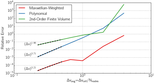
Figure 1: Relative error vs. velocity resolution for a Spitzer-Härm parallel heat flux problem, for 3 different algorithms: a standard 2cd-order finite volume method, DG with standard piecewise-linear basis functions, and DG with exponential-weighted piecewise-linear basis functions.

We developed a novel version of DG that uses exponentially-weighted (or Maxwellian-weighted) basis functions while still preserving exact particle and energy conservation. A key to preserving the conservation properties is the choice of weight in the inner product used for the error norm. Consider a general equation of the form $\partial f(v,t)/\partial t=G[f]$, where standard DG expands $f=\sum_{k}f_{k}(t)b_{k}(v)$ in each cell and chooses $\dot{f}_{k}=df_{k}/dt$ to minimize the error $\epsilon^{2}=\int dv(\sum_{k}\dot{f}_{k}b_{k}-G)^{2}$. While the standard conservation properties hold if polynomial basis functions are used, they are lost if the basis functions are exponential weighted, $b_{k}(v)=W(v)\hat{b}_{k}(v)$, where $W(v)=\exp(-\beta v^{2})$ and $\hat{b}_{k}$ are polynomials in $v$. Choosing $\dot{f}_{k}$ to minimize a weighted error defined as $\epsilon^{2}=\int dv(1/W(v))(\sum_{k}\dot{f}_{k}b_{k}-G)^{2}$ will then recover the standard conservation laws. Generalizations of this can be used to ensure positivity of $f(v,t)$. Basis functions capable of varying exponentially fast can represent certain features in the solution more efficiently, as demonstrated in Fig. 1 for a 1D test case involving parallel heat conduction, an important problem in the SOL. The Maxwellian-weighted DG method achieves the same error of $10^{-2}$ with 4 times fewer grid points in this 1D problem, which is 4 times less computational cost (assuming memory bandwidth is the limiting factor), or 16 times faster in the 2 velocity dimensions of gyrokinetics. This has been tested in a stand-alone code and future work can merge this into the main code.

Another approach that might lead to significant improvements in efficiency, particularly in higher dimensions, is use of sparse grid quadrature and fewer basis functions.

3 Formulation of model equations and boundary conditions

We have made a number of simplifying assumptions in the equations and the geometry for now in order to accelerate progress, but the physical model still retains key features of edge turbulence that have been computationally difficult in the past and are sufficient to demonstrate the overall feasibility of this approach. We have done simulations with a helical magnetic geometry (i.e., a toroidal and vertical magnetic field, such as in the Helimak and Torpex devices), which can be used as a simple model of the open-field line region of the scrape-off-layer in tokamaks. In this paper we focus on results just with a straight magnetic field such as in the LAPD device.

We use a gyrokinetic equation in the long wavelength limit with straight $\mathbf{B}$ field,

$$\frac{\partial f}{\partial t}+\frac{\partial}{\partial z}\left(v_{||}f\right)+\nabla\cdot\left(\vec{v}_{E}f\right)+\frac{\partial}{\partial v_{||}}\left(\frac{q}{m}E_{||}f\right)=C[f]+S$$ (1)

where $f(\vec{x},v_{||},\mu,t)$ is the guiding center distribution function, $\vec{v}_{E}$ is the $E\times B$ drift, $C[F]$ is a Lenard-Bernstein model collision operator, and $S$ is a source that balances losses to the end plates. The electric potential is determined by the long-wavelength gyrokinetic Poisson equation $-\nabla_{{\mbox{$\scriptscriptstyle\perp$}}}\cdot(\epsilon_{\mbox{$\scriptscriptstyle\perp$}}\nabla_{\mbox{$\scriptscriptstyle\perp$}}\phi)=\sum_{s}q\int d^{3}vf$, where $\epsilon_{\mbox{$\scriptscriptstyle\perp$}}(\vec{x})=c^{2}/v_{A0}^{2}=c^{2}4\pi n_{0}(\vec{x})m_{i}/B^{2}$ is the plasma perpendicular dielectric coefficient and is assumed to be time-independent for now. (This can be generalized to allow time varying density in $\epsilon_{\mbox{$\scriptscriptstyle\perp$}}$ if a second order contribution $-v_{E}^{2}$ to the Hamiltonian is kept.) The RHS of the gyrokinetic Poisson equation is the guiding center charge density $\sigma_{\rm gc}$, and the LHS is the negative of the polarization charge density.

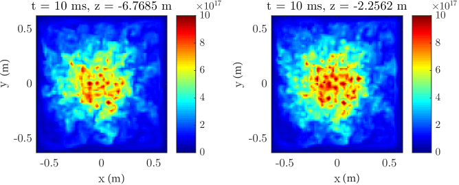
Figure 2: Contour plots of density fluctuations in the $(x,y)$ plane at two axial locations, from gyrokinetic turbulence simulations with the Gkeyll code, for parameters similar to the LAPD device (UCLA). Gkeyll uses advanced algorithms including discontinuous Galerkin methods methods to help with the computational challenges of edge turbulence.

When solving the gyrokinetic Poisson equation, we use the boundary conditions that $\phi=0$ on the side walls, at $x=0,L_{x}$ and $y=0,L_{y}$. (This also means that there is no $E\times B$ loss of guiding centers into the side walls, the only loss of guiding centers is to the end plates at $z=0,L_{z}$.) Given the guiding center charge density $\sigma_{\rm gc}(\vec{x})$, this then uniquely determines the potential $\phi(\vec{x})$ everywhere inside the plasma. If we start with a plasma that initially has $\sigma_{\rm gc}=0$ so $\phi=0$, then electrons will be lost to the end plates faster than ions. This leaves behind a net positive guiding center charge and causes $\phi$ to rise. Because the $\nabla_{\perp}$ in the gyrokinetic Poisson equation only involves perpendicular gradients, there will be a discontinuity between the positive potential in the plasma and $\phi=0$ on the end plates (assumed here to be grounded to the side walls). This jump represents the potential jump across the sheath region, which has a tiny width of order the Debye length, a scale along a field line that is not resolved in standard gyrokinetics. Electrons without enough parallel energy will be reflected back into the plasma (for a regular positive sheath). I.e., defining the sheath potential at $z=0$ as $\phi_{s}(x,y)=\lim_{\delta\rightarrow 0}\phi(x,y,\delta)$, we define a cutoff velocity $v_{c}(x,y)=\sqrt{2e\phi_{s}(x,y)/m_{e}}$ and impose the boundary condition for incoming electrons at $z=0$ as $f_{e}(x,y,0,v_{||},\mu,t)=f_{e}(x,y,0,-v_{||},\mu,t)$ for $0<v_{||}<v_{c}$, and $f_{e}(x,y,0,v_{||},\mu,t)=0$ for $v_{c}<v_{||}$. (There is no need for boundary conditions on the outgoing part of $f$ for $v_{||}<0$.)

These boundary conditions are the gyrokinetic equivalent of the boundary condition on electron fluid velocity used in early edge fluid turbulence simulations (such as [3, 6]), $V_{||e}=c_{s}\exp(\Lambda-e\phi_{s}/T_{e})$, though unlike the fluid case there is no assumption that the electrons are Maxwellian. The sheath potential will eventually rise until the mean electron flux is equal to the mean ion flux to the end plates, though these boundary conditions allow the net current at any particular location to fluctuate self-consistently, with return currents flowing through the wall. This differs from simple versions of a logical sheath that force $j_{||}=0$ everywhere on the end plate. There are various improvements to these boundary conditions that could be explored in the future, such as extensions for a magnetic pre-sheath for an inclined magnetic field [11, 12], extensions to better handle boundary layers that may form from polarization currents near the side walls, and modifications if the ion acceleration from the source region to the end plates is not large enough to exceed the Bohm sheath criterion. Extensions could eventually be made to treat some of the features of the LAPD experiment in more detail.

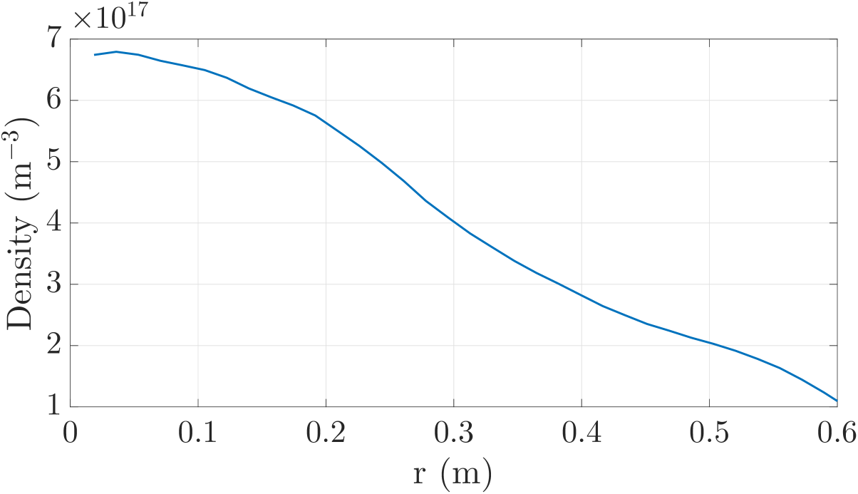
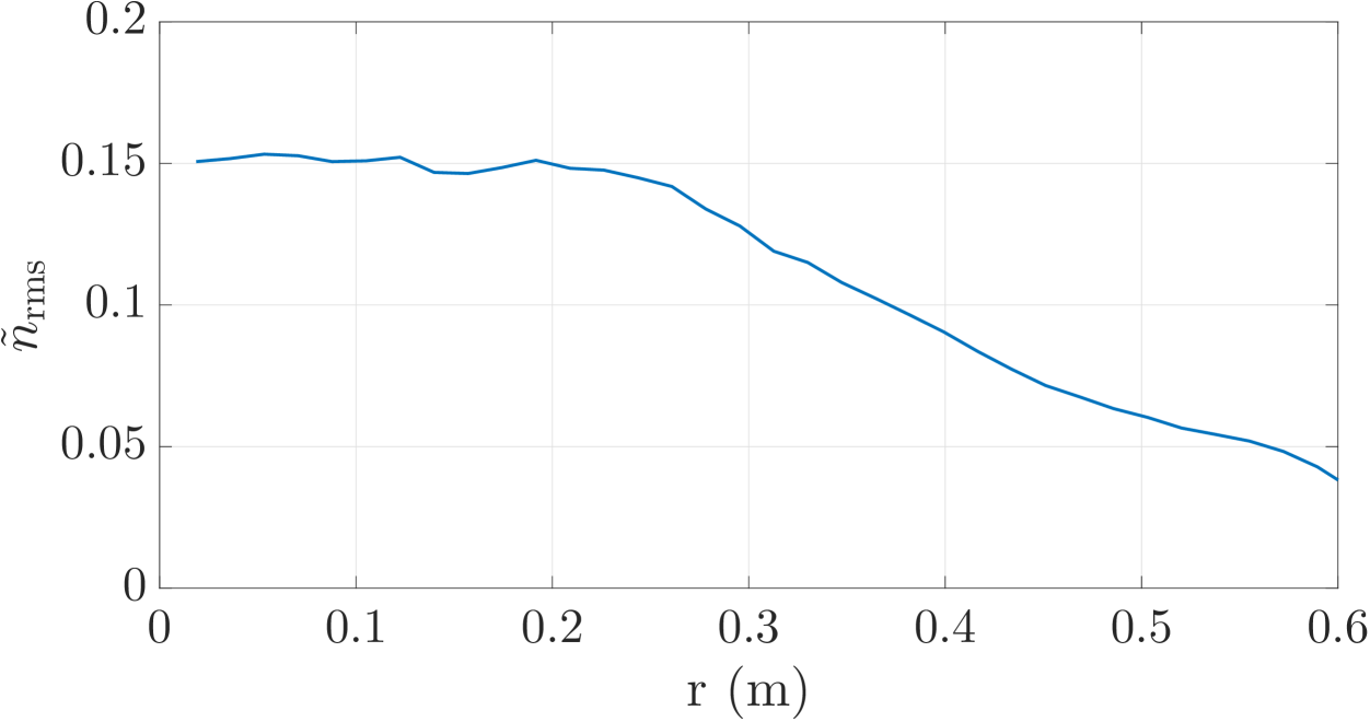
Figure 3: Radial profiles of the mean density $n_{0}(r)$ (left) and the rms density fluctuations (right, normalized to $n_{0}(0)$). The fluctuation amplitudes from these initial simulations are qualitatively similar to observations in LAPD. Future simulations will explore the impact of improved models of the LAPD source and setup.

For the above gyrokinetic equation and Poisson equation, one can show that the total energy $W_{\rm tot}=\sum_{s}\int d^{3}x\int d^{3}vf(1/2)mv_{||}^{2}+\int d^{3}x(\epsilon_{{\mbox{$\scriptscriptstyle\perp$}}}/8\pi)|\nabla_{\mbox{$\scriptscriptstyle\perp$}}\phi|^{2}$, which is the sum of parallel kinetic energy and perpendicular $E\times B$ flow energy, satisfies the equation

$$\frac{dW_{\rm tot}}{dt}=P_{S}-\int dS_{||}\sum_{s}\int d^{3}vf(1/2)mv_{||}^{3}-\int dS_{||}\phi j_{||}$$ (2)

where $\int dS_{||}$ represents an integral over the surface area of the parallel end plates, using the potential just inside the plasma at the entrance to the unresolved sheath region. On the RHS, the first term $P_{S}$ represents the input power from the source, the second term is the kinetic energy flux to the top of the sheath, and the third term represents the acceleration of ions and the deceleration of electrons by the sheath before they hit the wall. If the integrated $j_{||}$ through the sheath is non-zero, this implies the guiding center charge in the plasma is changing and it can put energy into $E\times B$ flows.

4 First Continuum Gyrokinetic Simulations of Edge Turbulence

The LArge Plasma Device LAPD[13, 14] is a linear plasma device that has been used to study a wide range of plasma phenomena including turbulent radial transport. It uses a hot cathode and mesh at one end that creates $\sim 50$ eV electrons that ionize and heat the plasma. Our code could eventually do a more detailed treatment of these processes, but for now we just use a fixed plasma source and model sheath boundary conditions as described in the previous section.

For our initial simulations, we mostly followed the setup used in the early fluid simulations of LAPD by Rogers and Ricci[3], with some variations. The typical sound speed $c_{s}=\sqrt{T_{e0}/m_{i}}=1.2\times 10^{4}$ m/s and sound gyroradius $\rho_{s}=c_{s}/\Omega_{ci}=1.25\times 10^{-2}$ m for $T_{e0}=6$ ev and the domain size was $(L_{x},L_{y},L_{z})=(1.25,1.25,18)$ m. The electron and ion sources were taken to be a Maxwellian in velocity with temperatures of close to $T_{Se}=6$ eV and $T_{Si}=1$ eV in the main fuelling region. These initial simulations were done with a resolution of $(N_{x},N_{y},N_{z},N_{v_{||}},N_{\mu})=72\times 72\times 8\times 12\times 6$ node points (piecewise linear basis functions were used with 2 nodes in each dimension per DG cell). More recent simulations used a resolution of $72\times 72\times 20\times 20\times 10$ (this gives 200 velocity grid points per spatial grid point).

A snapshot of the density profiles at two different $z$ locations is shown in Fig. 2, at $t=10$ ms (about 13 sound times $L_{z}/2c_{s}$). These fluctuation features are qualitatively similar to the fluid simulations in Ref.[3]. We have not yet included explicit viscosity, and ion-ion or ion-neutral viscosity may smooth the small scales some.

The mean density profile and the RMS density fluctuation amplitude profile is shown in Fig. 3. The latter is qualitatively similar to the observation of $\sim$10% fluctuations in the LAPD experiment reported in Fig. 2 of [6], but more detailed simulations for that specific experiment need to be done for careful comparisons.

5 Conclusions

We have presented first results from the Gkeyll code of 5D continuum gyrokinetic simulations on open field lines with model sheath boundary conditions. Results for LAPD are shown. We are using various simplifications at present, such as a simple helical magnetic field model, but this is sufficient to demonstrate the overall feasibility of this approach. This simplified system contains some of the key physics of the SOL region, such as the bad curvature drive of toroidal instabilities, rapid parallel losses to the divertor plates and interactions with sheaths, and so it can be useful to begin physics studies about the nature of SOL turbulence, such as why doesn’t this turbulence spread power more widely on divertor plates, and what are the effects of reduced recycling with lithium? There is some numerical heating in our present code from the correction step used to preserve positivity everywhere within a DG cell, and we are working on ways to improve this. There are a number of other ways that Gkeyll could be improved in the future, including exponentially-weighted basis functions or other algorithmic improvements, more detailed physics including atomic physics, and extensions to general geometry to handle open and closed field line regions simultaneously.

References

- [1] COCKBURN, B. et al., Journal of Scientific Computing 16 (2001) 173.
- [2] KU, S. et al., Journal of Computational Physics 315 (2016) 467 .
- [3] ROGERS, B. N. et al., Phys. Rev. Lett. 104 (2010) 225002.
- [4] RICCI, P. et al., Phys. Rev. Lett. 104 (2010) 145001.
- [5] POPOVICH, P. et al., Physics of Plasmas 17 (2010).
- [6] FRIEDMAN, B. et al., Physics of Plasmas 20 (2013).
- [7] LIU, J.-G. et al., Journal of Computational Physics 160 (2000) 577.
- [8] TAITANO, W. et al., J. Comput. Phys. 297 (2015) 357.
- [9] Hakim, A. H. et al., ArXiv e-prints (2014), http://arxiv.org/abs/1405.5907.
- [10] Shi, E. L. et al., Physics of Plasmas 22 (2015) 022504.
- [11] LOIZU, J. et al., Physics of Plasmas 19 (2012).
- [12] Geraldini, A. et al., ArXiv e-prints (2016).
- [13] GEKELMAN, W. et al., Review of Scientific Instruments 62 (1991) 2875.
- [14] CARTER, T. A. et al., Physics of Plasmas 16 (2009).