Data-driven time parallelism via forecasting

Abstract

This work proposes a data-driven method for enabling the efficient, stable time-parallel numerical solution of systems of ordinary differential equations (ODEs). The method assumes that low-dimensional bases that accurately capture the time evolution of the dynamical-system state are available; these bases can be computed from snapshot data by proper orthogonal decomposition (POD) in the case of parameterized ODEs, for example. The method adopts the parareal framework for time parallelism, which is defined by an initialization method, a coarse propagator that advances solutions on a coarse time grid, and a fine propagator that operates on an underlying fine time grid. Rather than employing usual approaches for initialization and coarse propagation (e.g., a typical time integrator applied with a large time step), we propose novel data-driven techniques that leverage the available time-evolution bases. The coarse propagator is defined by a forecast (proposed in Ref. [12]) applied locally within each coarse time interval, which comprises the following steps: (1) apply the fine propagator for a small number of time steps, (2) approximate the state over the entire coarse time interval using gappy POD with the local time-evolution bases, and (3) select the approximation at the end of the time interval as the propagated state. We also propose both local-forecast initialization (i.e., the local-forecast coarse propagator applied sequentially) and global-forecast initialization (i.e., the local-forecast coarse propagator applied over the entire time interval with global time-evolution bases). The method is particularly well suited for POD-based reduced-order models (ROMs). In this case, spatial parallelism quickly saturates, as the ROM dynamical system is low dimensional; thus, time parallelism is needed to enable lower wall times. Further, the time-evolution bases can be extracted from readily available data, i.e., the right singular vectors arising during POD computation. In addition to performing analyses related to the method’s accuracy, speedup, stability, and convergence, we also numerically demonstrate the method’s performance. Here, numerical experiments on ROMs for a nonlinear convection–reaction problem demonstrate the method’s ability to realize near-ideal speedups; global-forecast initialization with a local-forecast coarse propagator leads to the best performance.

1 Introduction

Two emerging trends introduce both challenges and opportunities in computational science: (1) in future extreme-scale architectures, improved wall-time performance must be achieved primarily by exposing additional concurrency, and (2) the rapid increase in the volume of available physical and computational data presents an opportunity to extract useful insights from these data. The first of these trends can be attributed to the stagnation of clock speeds and attendant increase in core counts; further, the execution time and energy-consumption costs of communication tend to dominate those of computation at extreme scale, thus creating an additional incentive for (communication-avoiding) concurrent computation. The second of these trends arises from an increase in both the number of sensors and in the quantity of generated data (e.g., particle-image-velocimetry measurement systems generate full spatio-temporal datasets), as well as the increasing fidelity of physics-based simulations, which generate large-scale computational datasets. Further, these trends expose a unique opportunity: integrating extreme-scale simulation with data analytics can positively impact both data-intensive science and extreme-scale computing [47].

This is what this work aims to accomplish: we aim to leverage available computational data to improve concurrency and parallel performance when simulating parameterized dynamical systems. More precisely, this work considers numerically solving large-scale systems of parameterized ordinary differential equations (ODEs), which arise in applications ranging from computational fluid dynamics to molecular dynamics. The above trends have particular implications in this context.

1.1 Numerically solving ODEs: exposing concurrency

First, the sequential nature of numerically solving ODEs (i.e., numerical time integration) typically poses the dominant computational bottleneck, both in strong and weak scaling. Strong scaling refers to increasing the number of computing cores used to solve a problem of fixed (total) size. In the context of numerically solving ODEs, strong scaling is typically achieved through parallelizing ‘across the system’ by increasing the number of processors over which the problem is decomposed spatially; this usually associates with parallelizing the linear-system solve occurring within each time step for implicit time integration. However, spatial parallelism saturates: there exists a number of cores beyond which the speedup decreases due to the dominance of latency and bandwidth costs over savings in sequential computation. This maximum number of (useful) cores is proportional to the problem size and defines the minimum wall-time achievable by spatial parallelism alone, even in the presence of unlimited computational resources. This wall-time floor can preclude computational models from being employed in time-critical applications (e.g., model predictive control, in-the-field analysis) that demand low simulation times. Weak scaling refers to simultaneously increasing both the number of computing cores and total problem size such that the problem size per core remains fixed. In the context of numerically solving ODEs, weak scaling is typically achieved by refining the spatial discretization (when the ODE associates with a spatially discretized partial differential equation) as the number of cores used for spatial parallelism increases. However, in order to prevent time-discretization errors from dominating spatial-discretization errors (and to preserve stability in the case of explicit time integration), spatial refinement typically requires attendant temporal refinement, which leads to an increase in the total number of time steps. This implies poor weak scaling, as the wall time is proportional to the problem size in this case.

To this end, researchers have developed a number of time-parallel methods that ‘widen the computational front’ by exposing parallelism in the temporal dimension. In principle, such approaches can mitigate this bottleneck, as they can decrease the minimum realizable wall time in the strong-scaling case, and can remove the dependence of the runtime on the total number of time steps in the weak-scaling case. Broadly, these techniques can be categorized [27] as iterative methods based on multiple shooting [42, 6, 45, 33, 23], domain decomposition and waveform relaxation [26, 48], and multigrid [31, 34, 32, 38, 19, 22, 40], as well as direct methods [39, 1, 50, 51, 46, 36].

Perhaps the most well-studied and widely adopted time-parallel method is the parareal technique [33], which can be interpreted [29, 22] as a deferred/residual-correction scheme, a multiple-shooting method with a finite-difference Jacobian approximation, or as a two-level multigrid method. The parareal method alternates between (1) time integration using a fine propagator executed in parallel on a non-overlapping decomposition of the time domain, and (2) time integration using a coarse propagator executed in serial on a coarse time discretization defined by boundaries of the temporal subdomains. The update formula associated with sequential coarse time integration aims to set the discontinuities in the fine solution (occurring at temporal-subdomain boundaries) to zero.

The parareal method converges to the solution computed by the fine propagator; thus the fine propagator is usually chosen to be a typical single-step time integrator (e.g., Runge–Kutta scheme). On the other hand, the coarse propagator can be chosen somewhat freely; it determines the parallel performance of the parareal method. Desired properties in the coarse propagator include accuracy (i.e., it should incur small error with respect to the fine propagator to ensure fast convergence), low cost (i.e., its computational complexity should not scale with the underlying fine time discretization), and stability (i.e., it should ensure a stable parareal recurrence). A primary research area within time-parallel methods aims to develop coarse propagators that satisfy these properties.

The most commonly used coarse propagator is simply a typical time integrator (which can have a lower-order accuracy than the fine propagator [7]) applied with coarse time steps [33, 4] or an explicit time integrator [41] (where stability may preclude use for large coarse time steps). While straightforward to implement, the coarse time step is typically outside the asymptotic range of convergence for the chosen time integrator, which can hamper accuracy and lead to slow parareal convergence. This approach can be accelerated by additionally coarsening the spatial discretization [25, 24, 17], employed simplified physics models [2, 37, 7, 20, 35], or relaxed solver tolerances [30]. Some authors have also employed reduced-order models constructed ‘on the fly’ (i.e., during the parareal recurrence without any ‘offline’ pre-processing step) [24, 17, 44, 14]. Instead, this work proposes employing time-evolution data that may be available to devise an accurate, low-cost, stable coarse propagator. We now describe the source of these data.

1.2 Numerically solving ODEs: availability of data

It is often the case that data are available about the dynamical system of interest. These data can arise (1) from experimental analyses, (2) from numerically solving the system of ODEs over a small time interval, or (3) from simulating the dynamical system for different parameter instances (if the dynamical system is parameterized), for example.

In this work, we assume that data are available related to the time evolution of the dynamical-system state. Such data may be extracted from any of the above sources. For example, these data could be provided from (1) experimental time traces of state variables at different spatial coordinates, (2) a time-domain Fourier transform of the short-time ODE numerical solution, or (3) the singular value decomposition (SVD) of the numerical spatio-temporal solution to the dynamical system at different parameter instances. While we focus primarily on the third data source (see Section 5), this is not strictly required for the method to be employed.

1.3 Proposed methodology

The proposed methodology adopts the data-driven forecasting method introduced in Ref. [12] to define both the coarse propagator and the initial solution used to ‘seed’ the parareal recurrence. Given bases for the time-evolution of the dynamical-system state (as discussed in Section 1.2 above), the coarse propagator is defined on a given coarse time interval by a ‘local forecast’ as follows: (1) apply the fine propagator for a small number of time steps, (2) apply gappy POD [21] with local time-evolution bases (with support over the coarse time interval) to generate an approximation of the state over the entire coarse time interval, and (3) select the value of the approximated state at the end of the coarse time interval as the propagated state. For initialization, this ‘local forecast’ can be applied sequentially; alternatively, a ‘global forecast’ can be applied as follows: (1) apply the fine propagator for a small number of time steps at the beginning of the time interval, (2) apply gappy POD with global time-evolution bases (with support over the entire time interval) to generate an approximation of the state over the entire time interval, and (3) select the value of the approximated state at the temporal-subdomain boundaries as the initial solution.

The methodology is particular well-suited for projection-based reduced-order models (ROMs) for two reasons. First, dynamical-system ROMs associate with small-scale ODEs that typically must be integrated over long time intervals. This occurs because ROMs reduce the spatial complexity (i.e., the cost of each linear-system solve) of large-scale dynamical systems by reducing the number of degrees of freedom (via projection) and complexity of evaluating nonlinear terms (e.g., via empirical interpolation [5, 13], empirical operator interpolation [18], or gappy POD [10]); however, ROMs generally do not significantly reduce the associated temporal complexity (i.e., the number of linear-system solves), which is typically proportional to the spatial dimension of the original large-scale dynamical system. Thus, ROMs suffer from early spatial-parallelism saturation associated with strong scaling as discussed in Section 1.1. For example, on a compressible flow problem, the Gauss–Newton with approximated tensors (GNAT) ROM yielded a 438 factor improvement as measured in core–hours, but only a 6.86 wall-time speedup [8]; spatial parallelism was saturated with only 12 cores. Second, ROMs already require computational data for their construction. In fact, ROMs based on proper orthogonal decomposition (POD) already employ the third data set described in Section 1.2; thus, the proposed coarse propagator can be computed ‘for free’ in such contexts (see Section 5.2). Here, the required time-evolution bases are easily obtained from the right singular vectors of corresponding snapshot matrices. Finally, we note that while we present the proposed coarse propagator and initialization methods in the parareal context, these techniques could also be applied to alternative time-parallel methods, e.g., PITA [23], MGRIT [22].

1.4 Outline and notation

To summarize, contributions of this work include:

• A novel coarse propagator based on local forecasting (Section 3.3),

• Novel initialization methods based on both local and global forecasting (Section 3.4),

• Error analysis for the local-forecast coarse propagator (Section 4.1) in the general (Theorem 1) and ideal (Theorem 3) cases,

• Speedup analysis for all proposed methods (Section 4.2) in the general (Theorems 4–5) and ideal (Theorems 6–7) cases,

• Stability analysis (Section 4.3) of the local-forecast coarse propagator (Lemma 9) and the resulting parareal recurrence (Theorem 11),

• Convergence analysis (Section 4.4) of the local-forecast coarse propagator within the parareal recurrence (Corollary 13),

• Descriptions of how the required method ingredients can be computed via POD (Section 5) for parameterized ODEs (Section 5.1) and reduced-order models (Section 5.2), and

• Numerical experiments (Section 6) that both highlight the practical benefits of the proposed methodology and illustrate the theoretical results.

The paper is structured as follows. Section 2 introduces the parareal method, Section 3 describes the proposed methodology, including algebraic techniques for data-driven global (Section 3.1) and local (Section 3.2) forecasting, and their application as coarse propagators (Section 3.3) and initialization methods (Section 3.4). Section 4 analyzes the proposed method in terms of accuracy (Section 4.1), cost/speedup (Section 4.2), stability (Section 4.3), and convergence (Section 4.4). Section 5 describes how the ingredients of the proposed methodology can be computed for parameterized ODEs (Section 5.1) and reduced-order models (Section 5.2) using proper orthogonal decomposition (POD), which is closely related to the singular value decomposition (SVD). Section 6 provides numerical experiments that assess the performance of the proposed technique in practice. Finally, Section 7 concludes the manuscript, Appendix A contains all proofs, Appendix B provides some additional aspects on using forecasting for Newton-initialization.

In the remainder of this paper, matrices are denoted by capitalized bold letters, vectors by lowercase bold letters, scalars by unbolded letters. The columns of a matrix ${\mathbf{A}}\in\mathbb{R}^{m\times{n}}$ are denoted by ${\mathbf{a}}_{i}\in\mathbb{R}^{m}$, $i\in{\rm Nature}{{n}}$ with ${\rm Nature}{n}\vcentcolon=\{1,\ldots,n\}$ such that ${\mathbf{A}}\vcentcolon=\left[{\mathbf{a}}_{1}\ \cdots\ {\mathbf{a}}_{n}\right]$. The scalar-valued matrix elements are denoted by $a_{i,j}\in\mathbb{R}$ such that ${\mathbf{a}}_{j}\vcentcolon=\left[a_{1,j}\ \cdots\ a_{m,j}\right]^{T}$, $j\in{\rm Nature}{{n}}$; we similarly denote the elements of a vector as ${\mathbf{a}}\vcentcolon=\left[a_{1}\ \cdots\ a_{m}\right]^{T}$. We also define $\mathbb{N}_{0}(n)\vcentcolon=\{0,\ldots,n\}$.

2 Time parallelism and parareal

We consider initial value problems for systems of (possibly nonlinear) ordinary differential equations (ODEs) of the form

(1) $$\frac{d}{dt}{{\mathbf{x}}^{\star}}(t) =\mathbf{g}\left({\mathbf{x}}^{\star};t\right),\quad{\mathbf{x}}^{\star}(0)={\mathbf{x}}^{0}\ ,$$

where $t\in[0,T_{\mathrm{final}}]$ denotes time with $T_{\mathrm{final}}\in\mathbb{R}_{+}{}$ the final time, ${\mathbf{x}}^{\star}:\mathbb{R}_{+}\rightarrow\mathbb{R}^{N}$ denotes the state implicitly defined as the (exact) solution to problem (1), ${\mathbf{x}}^{0}\in\mathbb{R}^{N}$ denotes the initial state, and $\mathbf{g}:\mathbb{R}^{N}\times\mathbb{R}_{+}\rightarrow\mathbb{R}^{N}$ with $({\boldsymbol{\xi}};{t})\mapsto\mathbf{g}({\boldsymbol{\xi}};{t})$ denotes the velocity, which may be linear or nonlinear in its first argument. Time-parallel methods constitute one approach to improve wall-time performance when numerically solving such problems. We now introduce the parareal method, which we consider in this work.

First, and without loss of generality, we introduce a uniform fine time discretization characterized by time step ${h}{=T_{\mathrm{final}}/m}$ and time instances $t^{{{n}}}={{n}}{h}$, ${{n}}\in\mathbb{N}_{0}(m)$, where $m\in\mathbb{N}$ denotes the number of total time instances beyond the initial time $t^{0}=0$ such that the final time corresponds to $t^{m}=T_{\mathrm{final}}$. We denote the set of time instances associated with this discretization as $\mathcal{t}\vcentcolon=\{t^{{{n}}}\}_{{{n}}=0}^{m}$. We introduce a ‘fine propagator’ $\mathcal{F}:\mathbb{R}^{N}\times\mathcal{t}\times\mathcal{t}\rightarrow\mathbb{R}^{N}$ with $({\boldsymbol{\xi}};{{t}^{i}},{{t}^{j}})\mapsto\mathcal{F}({\boldsymbol{\xi}};{{t}^{i}},{{t}^{j}})$ that acts on this discretization and propagates a state ${\boldsymbol{\xi}}\in\mathbb{R}^{N}$ defined at time ${{t}^{i}}$ to time ${{t}^{j}}$ with $j\geq i$. This propagator satisfies

(2) $${\mathcal{F}({\boldsymbol{\xi}};{{t}^{i}},{{t}^{k}})=\mathcal{F}(\cdot;{{t}^{j}},{{t}^{k}})\circ\mathcal{F}({\boldsymbol{\xi}};{{t}^{i}},{{t}^{j}}),\quad 0\leq i\leq j\leq k\leq m}$$

and typically corresponds to the application of a single-step time integrator (e.g., Runge–Kutta scheme) to numerically solve problem (1). For example, the backward-Euler fine propagator $\mathcal{F}_{\mathrm{BE}}$ implicitly satisfies $\mathcal{F}_{\mathrm{BE}}({\boldsymbol{\xi}};{{t}^{i}},{{t}^{i+1}})-{\boldsymbol{\xi}}-{h}\mathbf{g}\left(\mathcal{F}_{\mathrm{BE}}({\boldsymbol{\xi}};{{t}^{i}},{{t}^{i+1}});{{t}^{i+1}}\right)=0,\ i\in\mathbb{N}_{0}(m-1).$ We define

(3) $$\begin{split}{\mathbf{x}}&:{t}\mapsto\mathcal{F}({\mathbf{x}}^{0};0,{t}),\quad{{t}\in\mathcal{t}}\end{split}$$

as the associated numerical solution with ${\mathbf{x}}\in(\mathcal{H})^{N}$, where $\mathcal{H}$ denotes the set of functions from $\mathcal{t}$ to $\mathbb{R}$. Note that Eqs. (2) and (3) imply ${\mathbf{x}}(t^{j})=\mathcal{F}({\mathbf{x}}(t^{i});t^{i},t^{j}),\ 0\leq i\leq j\leq m$. It is this time-discrete solution ${\mathbf{x}}$, which we want to approximate with the time-parallel procedure.

Analogously, we consider a coarse time discretization characterized by (uniform) time step ${H}{=T_{\mathrm{final}}/{M}}$ and time instances ${T}^{{{n}}}={{n}}{H}$, ${{n}}\in\mathbb{N}_{0}({M})$, where ${M}\in\mathbb{N}$ denotes the number of coarse time instances beyond the initial time ${T}^{0}=t^{0}=0$ such that the final time corresponds to ${T}^{{M}}=t^{m}=T_{\mathrm{final}}$ (see Figure 1). We denote the set of time instances associated with the coarse discretization as $\mathcal{T}\vcentcolon=\{{T}^{{{n}}}\}_{{{n}}=0}^{{M}}$. Further, we assume that the coarse time step is an integral multiple of the fine time step, i.e., ${H}={\bar{m}}h$ with ${\bar{m}}\in\mathbb{N}$. This implies that the coarse discretization is nested within the fine discretization $\mathcal{T}\subseteq\mathcal{t}$ such that ${T}^{{{n}}}=t^{{{{\bar{m}}}}{{n}}}$, ${{n}}\in\mathbb{N}_{0}({M})$ and $m={\bar{m}}{M}$. We define the set of fine time instances associated with the ${{n}}$th coarse time interval as $\mathcal{t}^{{{n}}}\vcentcolon=\mathcal{t}\cap\left[{T}^{{{n}}},{T}^{{{n}}+1}\right]=\{t^{i}\}_{i={\bar{m}}{{n}}}^{{\bar{m}}({{n}}+1)}$, ${{n}}\in\mathbb{N}_{0}({M}-1)$.

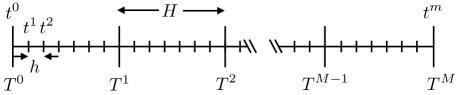
Fig. 1: Coarse and fine time discretizations.

Denoting by ${\mathbf{x}}^{{{{n}}}}_{{k}}$ the approximation to ${\mathbf{x}}({T}^{{{{n}}}})$ at parareal iteration ${k}$, the parareal method first computes an initial guess ${\mathbf{x}}^{{{n}}}_{0}$, ${{n}}\in\mathbb{N}_{0}({M}-1)$ with ${\mathbf{x}}^{0}_{0}={\mathbf{x}}^{0}$ (typically via ${\mathbf{x}}^{{{n}}+1}_{0}=\mathcal{G}({\mathbf{x}}^{{{{n}}}}_{0};{T}^{{{{n}}}},{T}^{{{{n}}}+1})$), and subsequently executes the following iterations

(4) $$\quad{\mathbf{x}}^{{{{n}}}+1}_{{k}+1}=\mathcal{G}({\mathbf{x}}^{{{{n}}}}_{{k}+1};{T}^{{{{n}}}},{T}^{{{{n}}}+1})+\mathcal{F}({\mathbf{x}}^{{{{n}}}}_{{k}};{T}^{{{{n}}}},{T}^{{{{n}}}+1})-\mathcal{G}({\mathbf{x}}^{{{{n}}}}_{{k}};{T}^{{{{n}}}},{T}^{{{{n}}}+1}),\ {k}=0,\ldots,{K},\ {{n}}={k},\ldots,{M}-1,$$

where ${\mathbf{x}}^{{k}}_{{k}+1}={\mathbf{x}}^{{k}}_{{k}}$ and ${K}$ is determined by a termination criterion that is satisfied when the solution discontinuities at coarse time instances become sufficiently small. Here, $\mathcal{G}:\mathbb{R}^{N}\times\mathcal{T}\times\mathcal{T}\rightarrow\mathbb{R}^{N}$ with $({\boldsymbol{\xi}};{T}^{i},{T}^{j})\mapsto\mathcal{G}({\boldsymbol{\xi}};{T}^{i},{T}^{j})$ denotes a ‘coarse propagator’ that propagates a state ${\boldsymbol{\xi}}$ defined at (coarse) time instance ${T}^{i}$ to time instance ${T}^{j}$ with $j>i$. In essence, the parareal method alternates serial (inexpensive) coarse propagation with parallel (expensive) fine propagation; the expectation is that parallelizing the fine propagation can realize wall-time performance improvements. Algorithm 1—which enables alternative initializations—reports the particular parareal algorithm we consider in this work.

Critically, this method exhibits the ‘finite-termination property’, which is the result

(5) $${\mathbf{x}}^{{{n}}}_{{k}}={\mathbf{x}}({T}^{{{n}}}),\quad{{n}}\leq{k}+1.$$

This states that the method will terminate in at most ${K}={M}-1$ parareal iterations; realizing this ‘worst-case scenario’ implies that the parallelization over time provided no gain over numerically solving Eq. (1) using the fine propagator in serial.

Algorithm 1 parareal_with_initialization

0:  Fine propagator $\mathcal{F}$, coarse propagator $\mathcal{G}$, initialization algorithm initialize, initial condition ${\mathbf{x}}^{0}_{0}$, termination tolerance $\epsilon$

0:  Number of parareal iterations ${K}\leftarrow{k}$, converged solution $({\mathbf{x}}^{1}_{0},\ldots,{\mathbf{x}}^{{K}+1}_{{K}},\ldots,{\mathbf{x}}^{{M}}_{{K}})$

1:   ${k}\leftarrow 0$

2:   $({\mathbf{x}}^{1}_{0},\ldots,{\mathbf{x}}^{{M}}_{0})=\texttt{initialize}({\mathbf{x}}^{0}_{0})$

3:  for ${{n}}=0,\ldots,{M}-1$ do {parallel fine propagation}

4:      ${{\mathbf{f}^{{{n}}+1}_{0}}}=\mathcal{F}({\mathbf{x}}^{{{n}}}_{0};{T}^{{{n}}},{T}^{{{n}}+1})$

5:  end for

6:  while $\max_{{{n}}\in\{{k}+1,\ldots,{M}-1\}}\|{{\mathbf{f}^{{{n}}}_{{k}}}}-{\mathbf{x}}^{{{n}}}_{{k}}\|/\|{{\mathbf{f}^{{{n}}}_{{k}}}}\|>\epsilon$ do

7:     if ${k}=0$ then {initial-seed coarse propagation}

8:        for ${{n}}=1,\ldots,{M}-1$ do {parallel coarse propagation}

9:            $\mathbf{g}^{{{n}}+1}_{0}=\mathcal{G}({\mathbf{x}}^{{{n}}}_{0};{T}^{{{n}}},{T}^{{{n}}+1})$

10:        end for

11:     end if

12:      ${\mathbf{x}}^{{k}}_{{k}+1}={\mathbf{x}}^{{k}}_{{k}}$

13:     for ${{n}}={k},\ldots,{M}-1$ do {serial coarse propagation and correction}

14:         $\mathbf{g}^{{{n}}+1}_{{k}+1}=\mathcal{G}({\mathbf{x}}^{{{n}}}_{{k}+1};{T}^{{{n}}},{T}^{{{n}}+1})$

15:         ${\mathbf{x}}^{{{n}}+1}_{{k}+1}=\mathbf{g}^{{{n}}+1}_{{k}+1}+{{\mathbf{f}^{{{n}}+1}_{{k}}}}-\mathbf{g}^{{{n}}+1}_{{k}}$

16:     end for

17:     for ${{n}}={k},\ldots,{M}-1$ do {parallel fine propagation}

18:         ${{\mathbf{f}^{{{n}}+1}_{{k}+1}}}=\mathcal{F}({\mathbf{x}}^{{{n}}}_{{k}+1};{T}^{{{n}}},{T}^{{{n}}+1})$

19:     end for

20:     ${k}\leftarrow{k}+1$

21:  end while

22:  for ${{n}}={k},\ldots,{M}-1$ do

23:      ${\mathbf{x}}^{{{n}}+1}_{{k}}\leftarrow{{\mathbf{f}^{{{n}}+1}_{{k}}}}$

24:  end for

3 Data-driven time parallelism

The objective of this work is to devise inputs to Algorithm 1 that leverage the availability of data that inform the time evolution of the state. Our two primary points of focus are (1) to devise an initialization method that yields an accurate initial guess, and (2) to develop a coarse propagator that is fast, accurate, and stable. In particular, we aim to improve upon the performance of existing techniques, which generally employ coarse propagators and initialization techniques that do not exploit time-evolution data that may be available.

Our critical assumption is that we have access to time-evolution bases $\mathbf{\Xi}_{j}\in\mathbb{V}_{{a}}(\mathbb{R}^{m})$, $j\in{\rm Nature}{N}$ with ${a}\leq m$ that describe the time evolution of the $j$th state ${x}_{j}$. Here, $\mathbb{V}_{{{n}}}(\mathbb{R}^{N}){\subset}\mathbb{R}^{N\times{{n}}}$ denotes the Stiefel manifold, i.e., the set of all real-valued $N\times{{n}}$ matrices with orthonormal columns. Subsequent sections will describe how these bases can be computed in the case of parameterized ODEs (Section 5.1) and projection-based reduced-order models (Section 5.2); for now, we simply assume that these bases are available and for ease of notation all have identical dimension ${a}$.

3.1 Global forecasting

We begin by summarizing the data-driven forecasting method proposed in Ref. [12]. Given bases $\mathbf{\Xi}_{j}$, $j\in{\rm Nature}{N}$ and a time instance ${i}\in{\rm Nature}{m}$, the forecasting approach approximates the time evolution of state variable ${x}_{j}$ via gappy POD using the basis $\mathbf{\Xi}_{j}$ and the value of ${x}_{j}$ at the most recent $\alpha$ time instances. Here, $\alpha\in\mathbb{N}$ with $\alpha\geq{a}$ denotes the ‘memory’, which will be considered a global variable in this manuscript. First, the method computes the gappy POD approximation ${\mathbf{w}}_{j}({x}_{j};t^{{i}})$, defined as

(6) $${\mathbf{w}}_{j}{({y};{{t}^{{i}}})=}\underset{{{\mathbf{w}}\in\mathrm{Ran}(\mathbf{\Xi}_{j})}}{\arg\min}\|{{\mathbf{Z}}_{{i}}}{\mathbf{w}}-{{\mathbf{Z}}_{{i}}}{\mathbf{h}}({y})\|_{2}={\mathbf{\Xi}_{j}}[{{\mathbf{Z}}_{{i}}}\mathbf{\Xi}_{j}]^{+}{{\mathbf{Z}}_{{i}}}{\mathbf{h}}({y}){,{\quad i\in\mathbb{N}_{0}(m-\alpha)},\,y\in\mathcal{H},}$$

where the superscript + denotes the Moore–Penrose pseudoinverse, $\mathrm{Ran}({{\mathbf{A}}})$ denotes the range of the matrix ${{\mathbf{A}}}$, and ${\mathbf{w}}_{j}:\mathcal{H}\times\mathcal{t}\rightarrow\mathbb{R}^{{m}}$. Here, the sampling matrix ${{\mathbf{Z}}_{i}}\vcentcolon=\begin{bmatrix}\mathbf{e}_{i+1}\ \cdots\ \mathbf{e}_{i+\alpha}\end{bmatrix}^{T}\in\{0,1\}^{\alpha\times m}$ extracts entries $i+1$ through $i+\alpha$ of a given vector and $\mathbf{e}_{i}\in\{0,1\}^{m}$ denotes the $i$th canonical unit vector. Further, $\mathbf{h}:\mathcal{H}\rightarrow\mathbb{R}^{m}$ centers and ‘unrolls’ a time-dependent variable according to the time discretization as

(7) $$\mathbf{h}:{{y}}\mapsto\left[{y}(t^{1})-{y}(t^{0})\ \cdots\ {y}(t^{m})-{y}(t^{0})\right]^{T}.$$

Then, the forecast at a given time instance ${{n}}$, which aims to approximate the value ${{x}_{j}}(t^{{{n}}})$, is set to ${f}_{j}({x}_{j};t^{{i}},t^{{{n}}})$, where we have defined the function that forecasts the time-dependent variable ${y}$ to time ${{t}^{k}}$ using its value at times ${{t}^{{i}+{\ell}}}$, ${\ell}\in{\rm Nature}{\alpha}$ as

(8) $${f}_{j}:({y};{{t}^{{i}}},{{t}^{k}})\mapsto{y}(0)+\mathbf{e}_{k}^{T}{\mathbf{w}}_{j}({y};{{t}^{{i}}}){,}{\quad i\in\mathbb{N}_{0}(m-\alpha),\,k\in\mathbb{N}_{0}(m),\,y\in\mathcal{H},}$$

with ${f}_{j}:\mathcal{H}\times\mathcal{t}\times\mathcal{t}\rightarrow\mathbb{R}$. Figure 2(a) illustrates the global-forecasting method graphically, and Algorithm 2 provides an algorithmic description of the method such that

$${f}_{j}({y};{{t}^{i}},{{t}^{k}})={\texttt{global\_forecast}}(\mathbf{\Xi}_{j},{y}(0),\{{y}({{t}^{\ell}})\}_{\ell=i+1}^{i+\alpha},i,k).$$

Algorithm 2 global_forecast (algorithmic description of the global forecast (8))

0:  time-evolution basis $\mathbf{\Xi}_{j}\in\mathbb{V}_{{a}}(\mathbb{R}^{m})$, initial state ${y}(0)\in\mathbb{R}$, sampled state $\{{y}({{t}^{\ell}})\}_{\ell=i+1}^{i+\alpha}\subset\mathbb{R}$, initial sampling time index $i\in\mathbb{N}_{0}(m-\alpha)$, forecast time index $k\in\mathbb{N}_{0}(m)$

0:  global forecast ${f}_{j}({y};{{t}^{i}},{{t}^{k}})\in\mathbb{R}$

1:  Solve gappy POD linear least-squares problem (6) for ${\mathbf{w}}_{j}({y};{{t}^{i}})\in\mathbb{R}^{m}$, noting that ${{\mathbf{Z}}_{i}}{\mathbf{h}}({y})=\left[{y}({{t}^{i+1}})-{y}(0),\cdots,{y}({{t}^{i+\alpha}})-{y}(0)\right]^{T}$. Note that the gappy POD approximation over all time is ${\mathbf{h}}({f}({y};{{t}^{i}},\cdot))=\mathbf{1}_{m}{y}(0)+{\mathbf{w}}_{j}({y};{{t}^{i}})$, where $\mathbf{1}_{m}$ denotes an $m$-vector of ones.

2:  Extract forecast at time instance ${{t}^{k}}$ via Eq. (8) as ${{f}_{j}({y};{{t}^{i}},{{t}^{k}})}=\mathbf{e}_{k}^{T}{\mathbf{h}}({f}_{j}({y};{{t}^{i}},\cdot))={y}(0)+\mathbf{e}_{k}^{T}{\mathbf{w}}_{j}({y};{{t}^{i}}).$

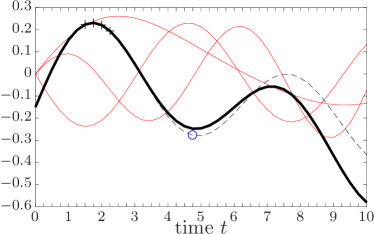
(a) Global forecast. Here, the time evolution basis vectors (i.e., columns of $\mathbf{\Xi}_{j}$) are denoted by thin colored lines, the state entry ${x}_{j}$ is denoted by a thick black line, the sampled state ${{\mathbf{Z}}_{i}}{\mathbf{h}}({x}_{j})+{x}_{j}(t^{0})$ is denoted by + markers, the forecast ${f}_{j}({x}_{j};{{t}^{i}},\cdot)$ with $i=5$ is plotted as dashed line and the forecast ${f}_{j}({x}_{j};{{t}^{i}},{{t}^{j}})$ for $j=19$ is denoted by a $\circ$ marker.

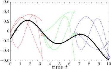
(b) Local forecast with ${M}=3$ coarse time intervals. Here, the time evolution basis vectors (i.e., columns of $\mathbf{\Xi}_{j}^{{n}}$) are denoted by thin colored lines, the state entry ${x}_{j}$ is denoted by a thick black line, the sampled state ${{\mathbf{Z}}_{0}}{\mathbf{h}^{{n}}}({x}_{j})+{x}_{j}({T}^{{{n}}})$ is denoted by + markers, and the forecast ${f}_{j}^{{n}}({x}_{j};{T}^{{{n}}},{T}^{{{n}}+1})$ is denoted by $\circ$ markers.

    

Fig. 2: Illustration of global and local forecasting with memory $\alpha=4$, time-evolution basis dimension ${a}=3$, final time $T_{\mathrm{final}}=10$, and time step ${h}=0.25$.

The approach proposed in Ref. [12] employed the forecast ${f}_{j}({x}_{j};t^{{i}},t^{{{n}}})$, $j\in{\rm Nature}{N}$ as an initial guess for the Newton solver at time $t^{{{n}}}$ for ${{n}}>{i}+\alpha$ obtained after discretizing the ODE associated with a ROM using a linear multistep scheme. Instead, this work considers employing this forecasting strategy to define both the initialization and coarse propagator as inputs to parareal Algorithm 1. We now propose a local variant of this global forecasting method that operates within a single coarse time interval.

3.2 Local forecasting

Algorithm 3 local_basis

0:  time-evolution basis ${\mathbf{\Xi}_{j}}\in\mathbb{V}_{{a}}(\mathbb{R}^{m})$, coarse-time-interval index ${{n}}\in\mathbb{N}_{0}({M}-1)$, energy criterion $\upsilon\in\left[0,1\right]$

0:  local time-evolution basis ${\mathbf{\Xi}_{j}^{{n}}}\in\mathbb{V}_{{a}}(\mathbb{R}^{{\bar{m}}})$

1:  ${\mathbf{\Xi}_{j}^{{n}}}\leftarrow{\mathbf{Z}}^{{{n}}}{\mathbf{\Xi}_{j}}$ {Extract values on ${{n}}$th coarse time interval}

2:  ${(\mathbf{U},\mathbf{\Sigma},\mathbf{V})}=\texttt{thin\_SVD}({\mathbf{\Xi}_{j}^{{n}}})$ {Compute (thin) singular value decomposition}

3:   ${\mathbf{\Xi}_{j}^{{n}}}\leftarrow\begin{bmatrix}\mathbf{u}_{1}\ \cdots\ \mathbf{u}_{{a}}\end{bmatrix}$, where ${a}=\min_{i\in{\Upsilon}(\upsilon)}i$, ${\Upsilon{(\upsilon)}}\vcentcolon=\{i\ |\ \sum_{\ell=1}^{i}{\sigma_{\ell}}/\sum_{k=1}^{a}{\sigma_{k}}\geq\upsilon\}$, ${\mathbf{\Sigma}}=\mathrm{diag}({\sigma_{1}},\ldots,{\sigma_{a}})$, ${\mathbf{U}}=\begin{bmatrix}{\mathbf{u}}_{1}\ \cdots\ {\mathbf{u}}_{a}\end{bmatrix}$. {Truncate}

The proposed local forecasting approach relies on local time-evolution bases $\mathbf{\Xi}_{j}^{{n}}\in\mathbb{V}_{{a}}(\mathbb{R}^{{\bar{m}}})$, $j\in{\rm Nature}{N}$ that inform the time evolution of the $j$th state ${x}_{j}$ over time interval $[{T}^{{{n}}},{T}^{{{n}}+1}]$. Given a (global) time-evolution basis $\mathbf{\Xi}_{j}$, these local bases $\mathbf{\Xi}_{j}^{{n}}$, ${{n}}\in\mathbb{N}_{0}({M}-1)$ can be computed via Algorithm 3 as $\mathbf{\Xi}_{j}^{{n}}={{\texttt{local\_basis}}}(\mathbf{\Xi}_{j},{{n}},\upsilon)$, where $\upsilon\in[0,1]$ defines a statistical ‘energy criterion’ and we have defined ${\mathbf{Z}}^{{{n}}}\vcentcolon=[\mathbf{e}_{{{{\bar{m}}}}{{n}}+1}\ \cdots\ \mathbf{e}_{{{{\bar{m}}}}{{n}}+1}]^{T}-\mathbf{1}_{{\bar{m}}}[\mathbf{e}_{{{{\bar{m}}}}{{n}}}]^{T}\in\{0,1\}^{{\bar{m}}\times m}$ as the matrix that samples entries associated with the ${{n}}$th coarse time interval and subtracts the initial value on that time interval. Here, $\mathbf{1}_{i}$ denotes an $i$-vector of ones. Note that truncation in Step 3 of Algorithm 3 ensures that the local basis $\mathbf{\Xi}_{j}^{{n}}$ will have full column rank. Using these local time-evolution bases (which have zero values at the beginning of their respective time intervals), we can define the local forecast using a similar construction to that of Section 3.1. In particular, the linear least-squares problem for the locally defined gappy POD approximation becomes

(9) $$\begin{split}{\mathbf{w}}_{j}^{{n}}{({y};{{t}^{i}})=}&\underset{{\mathbf{w}}\in{\mathrm{Ran}(\mathbf{\Xi}_{j}^{{n}})}}{\arg\min}\|{{\mathbf{Z}}_{i-{{{\bar{m}}}}{{n}}}}{\mathbf{w}}-{{\mathbf{Z}}_{i-{{{\bar{m}}}}{{n}}}}{\mathbf{h}^{{n}}}({y})\|_{2}=\mathbf{\Xi}_{j}^{{n}}[{{\mathbf{Z}}_{i-{{{\bar{m}}}}{{n}}}}\mathbf{\Xi}_{j}^{{n}}]^{+}{{\mathbf{Z}}_{i-{{{\bar{m}}}}{{n}}}}{\mathbf{h}^{{n}}}({y})\end{split}$$

for ${{t}^{i+\ell}}\in\mathcal{t}^{{{n}}}{,}\ \forall\ell\in{\rm Nature}{\alpha}$, with ${\mathbf{w}}_{j}^{{n}}:\mathcal{H}^{{{n}}}\times\mathcal{t}^{{{n}}}\rightarrow\mathbb{R}^{{\bar{m}}}$, where $\mathcal{H}^{{{n}}}$, ${{n}}\in\mathbb{N}_{0}({M}-1)$ denotes the set of functions from $\mathcal{t}^{{{n}}}$ to $\mathbb{R}$. Here, the function $\mathbf{h}^{{n}}:\mathcal{H}^{{{n}}}\rightarrow\mathbb{R}^{{\bar{m}}}$ locally centers and unrolls a time-dependent variable over the ${{n}}$th time interval as

(10) $$\mathbf{h}^{{n}}:{{y}}\mapsto\left[{y}(t^{{{{\bar{m}}}}{{n}}+1})-{y}({T}^{{{n}}})\ \cdots\ {y}({T}^{{{n}}+1})-{y}({T}^{{{n}}})\right]^{T}.$$

Note that if ${y}\in\mathcal{H}$, then ${\mathbf{h}^{{n}}}({y})={\mathbf{Z}}^{{{n}}}{\mathbf{h}}({y})$. Then, the function ${f}_{j}^{{n}}$ that forecasts a local time-dependent variable to time ${{t}^{{k}}}$ using the value of the variable at times ${{t}^{i+p}}$, $p\in{\rm Nature}{\alpha}$ can be defined algebraically as

(11) $$\begin{split}{f}_{j}^{{n}}&:({y};{{t}^{i}},{{t}^{{k}}})\mapsto{y}({T}^{{{n}}})+\mathbf{e}_{{k}-{{{\bar{m}}}}{{n}}}^{T}{\mathbf{w}}_{j}^{{n}}({y};{{t}^{i}}),\quad{{t}^{{k}}},{{t}^{i+\ell}}\in\mathcal{t}^{{{n}}}{,}\ \forall\ell\in{\rm Nature}{\alpha}\end{split}$$

with ${f}_{j}^{{n}}:\mathcal{H}^{{{n}}}\times\mathcal{t}^{{{n}}}\times\mathcal{t}^{{{n}}}\rightarrow\mathbb{R}$. Figure 2(b) illustrates the local-forecasting method graphically, and Algorithm 4 provides an algorithmic description of the method such that

$${f}_{j}^{{n}}({y};{{t}^{i}},{{t}^{k}})={\texttt{local\_forecast}}({{n}},\mathbf{\Xi}_{j}^{{n}},{y}({T}^{{{n}}}),\{{y}({{t}^{\ell}})\}_{\ell=i+1}^{i+\alpha},i,k).$$

Algorithm 4 local_forecast (algorithmic description of the local forecast (11))

0:  time interval index ${{n}}\in\mathbb{N}_{0}({M}-1)$, time-evolution basis $\mathbf{\Xi}_{j}^{{n}}\in\mathbb{V}_{{a}}(\mathbb{R}^{{\bar{m}}})$, state at beginning of time interval ${y}({T}^{{{n}}})\in\mathbb{R}$, sampled state $\{{y}({{t}^{\ell}})\}_{\ell=i+1}^{i+\alpha}\subset\mathbb{R}$, initial sampling time index $i\in\{{\bar{m}}{{n}},\ldots,{\bar{m}}({{n}}+1)-\alpha\}$, forecast time index $k\in\{{\bar{m}}{{n}},\ldots,{\bar{m}}({{n}}+1)\}$

0:  local forecast ${f}_{j}^{{n}}({y};{{t}^{i}},{{t}^{k}})\in\mathbb{R}$

1:  Solve gappy POD linear least-squares problem (9) for ${\mathbf{w}}_{j}^{{n}}({y};{{t}^{i}})$, noting that ${{\mathbf{Z}}_{i-{{{\bar{m}}}}{{n}}}}{\mathbf{h}^{{n}}}({y})=\left[{y}({{t}^{i+1}})-{y}({T}^{{{n}}}),\cdots,{y}({{t}^{i+\alpha}})-{y}({T}^{{{n}}})\right]^{T}$. Note that the gappy POD approximation over ${{n}}$th time interval is ${\mathbf{h}^{{n}}}({f}_{j}^{{n}}({y};{{t}^{i}},\cdot))=\mathbf{1}_{{\bar{m}}}{y}({T}^{{{n}}})+{\mathbf{w}}_{j}^{{n}}({y};{{t}^{i}})$.

2:  Extract forecast at time instance ${{t}^{k}}$ via Eq. (11) as ${{f}_{j}^{{n}}({y};{{t}^{i}},{{t}^{k}})}=\mathbf{e}_{k-{{{\bar{m}}}}{{n}}}^{T}{\mathbf{h}^{{n}}}({f}_{j}^{{n}}({y};{{t}^{i}},\cdot))={y}({T}^{{{n}}})+\mathbf{e}_{k-{{{\bar{m}}}}{{n}}}^{T}{\mathbf{w}}_{j}^{{n}}({y};{{t}^{i}}).$

3.3 Coarse propagator: local forecast

We aim to employ the local forecasting approach to construct a data-driven coarse propagator to be used in the parareal Algorithm 1. In particular, we propose to construct a propagator that maps the state evaluated at the first $\alpha$ fine time instances of a given coarse time interval to an approximation of the state at the final time of the coarse time interval. However, inspired by the multigrid interpretation of parareal, we acknowledge that the role of the coarse propagator is to reduce large-wavelength errors; thus we allow the technique to apply this propagation only to a restriction of the state. That is, we set the coarse propagation of the $j$th element of a restricted time-dependent vector to be the mapping

(12) $$\begin{split}{\boldsymbol{y}}\mapsto{f}_{j}^{{n}}({\mathbf{r}^{T}_{j}}{\boldsymbol{y}};{T}^{{{n}}},{T}^{{{n}}+1}):(\mathcal{H}^{{{n}}})^{N}\rightarrow\mathbb{R},\end{split}$$

where ${\mathbf{R}}\vcentcolon=\left[{\mathbf{r}_{1}}\ \cdots\ {\mathbf{r}_{{\bar{N}}}}\right]\in\mathbb{R}^{N\times{\bar{N}}}$ with ${\bar{N}}{\in{\rm Nature}{N}}$ denotes a (linear) restriction operator with associated prolongation operator ${\mathbf{P}}\in\mathbb{R}^{N\times{\bar{N}}}$. Note that the time-evolution bases should therefore be constructed to capture the time-evolution of the restricted time-dependent variable. Possible choices for the restriction operator include projection onto large-wavelength Fourier modes or onto a set of high-energy POD modes; the latter choice is natural for reduced-order models and is explored in the numerical experiments.

Introducing a function that maps a vector at the beginning of a coarse time interval to a function over the fine time discretization within that interval, i.e., $\mathcal{f}^{{{n}}}:{\boldsymbol{\xi}}\mapsto\mathcal{F}({\boldsymbol{\xi}};{T}^{{{n}}},\cdot)$ with $\mathcal{f}^{{{n}}}:\mathbb{R}^{N}\rightarrow(\mathcal{H}^{{{n}}})^{N}$, we define coarse propagation of the $j$th element of the restricted state on coarse time interval ${{n}}$ to be

(13) $$\begin{split}{\mathcal{G}_{\mathrm{LF}}}_{j}^{{{n}}}&:{\boldsymbol{\xi}}\mapsto{f}_{j}^{{n}}({\mathbf{r}^{T}_{j}}{\mathcal{f}^{{{n}}}({\boldsymbol{\xi}})};{T}^{{{n}}},{T}^{{{n}}+1}),\quad{{n}}\in\mathbb{N}_{0}({M}-1)\end{split}$$

with ${\mathcal{G}_{\mathrm{LF}}}_{j}^{{{n}}}:\mathbb{R}^{N}\rightarrow\mathbb{R}$, which can be expressed algebraically as

(14) $$\begin{split}{\mathcal{G}_{\mathrm{LF}}}_{j}^{{{n}}}&:{\boldsymbol{\xi}}\mapsto{\mathbf{r}^{T}_{j}}{\boldsymbol{\xi}}+\sum_{i=1}^{\alpha}{\gamma}_{ij}^{{n}}({\mathbf{r}^{T}_{j}}\mathcal{F}({\boldsymbol{\xi}};{T}^{{{n}}},t^{{{{\bar{m}}}}{{n}}+i})-{\mathbf{r}^{T}_{j}}{\boldsymbol{\xi}}),\quad{{n}}\in\mathbb{N}_{0}({M}-1)\end{split}$$

with ${\gamma}_{ij}^{{n}}\vcentcolon=\mathbf{e}_{{\bar{m}}}^{T}\mathbf{\Xi}_{j}^{{n}}\left[{{\mathbf{Z}}_{0}}\mathbf{\Xi}_{j}^{{n}}\right]^{+}\mathbf{e}_{i}\in\mathbb{R}$. We then propose employing a coarse propagator $\mathcal{G}\leftarrow{\mathcal{G}_{\mathrm{LF}}}$ with

(15) $$\begin{split}{\mathcal{G}_{\mathrm{LF}}}&:({\boldsymbol{\xi}};{T}^{{{n}}},{T}^{{{n}}+1})\mapsto{\mathbf{P}}\left[{\mathcal{G}_{\mathrm{LF}}}_{1}^{{{n}}}({\boldsymbol{\xi}})\ \cdots\ {\mathcal{G}_{\mathrm{LF}}}_{{\bar{N}}}^{{{n}}}({\boldsymbol{\xi}})\right]^{T}\end{split}$$

with ${\mathcal{G}_{\mathrm{LF}}}:\mathbb{R}^{N}\times\mathcal{T}\times\mathcal{T}\rightarrow\mathbb{R}^{N}$, which can be expressed algebraically as

(16) $${\mathcal{G}_{\mathrm{LF}}}:({\boldsymbol{\xi}};{T}^{{{{n}}}},{T}^{{{{n}}}+1})\mapsto{\mathbf{P}}{\mathbf{R}^{T}}{\boldsymbol{\xi}}+{\mathbf{P}}\sum_{i=1}^{\alpha}{{\mathbf{\Gamma}}_{i}^{{n}}}\left[{\mathbf{R}^{T}}\mathcal{F}({\boldsymbol{\xi}};{T}^{{{n}}},t^{{{{\bar{m}}}}{{n}}+i})-{\mathbf{R}^{T}}{\boldsymbol{\xi}}\right].$$

Here, we have defined ${{\mathbf{\Gamma}}_{i}^{{n}}}\vcentcolon=\mathop{\operator@font diag}\nolimits({\gamma}_{i1}^{{n}},\ldots,{\gamma}_{i{\bar{N}}}^{{n}})\in\mathbb{R}^{{\bar{N}}\times{\bar{N}}}$.

3.4 Initialization: local and global forecasts

Initialization in Step 2 of Algorithm 1 is typically executed by sequentially applying the coarse propagator, i.e.,

(17) $${\mathbf{x}}^{{{n}}+1}_{0}=\mathcal{G}({\mathbf{x}}^{{{n}}}_{0};{T}^{{{n}}},{T}^{{{n}}+1}),\quad{{n}}=0,\ldots,{M}-1.$$

This approach could be applied with the proposed local-forecasting coarse propagator $\mathcal{G}\leftarrow{\mathcal{G}_{\mathrm{LF}}}$. However, we can also consider an alternative initialization that is both computationally less expensive and more stable (as will be further discussed in Remark 4.6).

In particular, we consider performing initialization by forecasting the state from the first $\alpha$ time steps of the first time interval to all coarse time instances using the global time-evolution bases $\mathbf{\Xi}_{j}$. That is, we can perform initialization via global forecasting as

(18) $${\mathbf{x}}^{{{n}}+1}_{0}=\mathcal{G}_{\mathrm{GF}}({\mathbf{x}}^{0}_{0};{T}^{{{n}}+1}),\quad{{n}}=0,\ldots,{M}-1,$$

where we have defined

(19) $$\begin{split}\mathcal{G}_{\mathrm{GF}}&:({\boldsymbol{\xi}};{T}^{{{{n}}}})\mapsto{\mathbf{P}}[{f}_{1}({\mathbf{r}^{T}_{1}}\mathcal{f}({\boldsymbol{\xi}});{T}^{0},{T}^{{{n}}})\ \cdots\ {f}_{{\bar{N}}}({\mathbf{r}^{T}_{{\bar{N}}}}\mathcal{f}({\boldsymbol{\xi}});{T}^{0},{T}^{{{n}}})]^{T}\end{split}$$

with $\mathcal{G}_{\mathrm{GF}}:\mathbb{R}^{N}\times\mathcal{T}\rightarrow\mathbb{R}^{N}$, and $\mathcal{f}({\boldsymbol{\xi}}):{\boldsymbol{\xi}}\mapsto\mathcal{F}({\boldsymbol{\xi}};t^{0},\cdot)$ with $\mathcal{f}({\boldsymbol{\xi}}):\mathbb{R}^{N}\rightarrow(\mathcal{H})^{N}$, which can be expressed algebraically as

(20) $$\mathcal{G}_{\mathrm{GF}}:({\boldsymbol{\xi}};{T}^{{{{n}}}})\mapsto{\mathbf{P}}{\mathbf{R}^{T}}{\boldsymbol{\xi}}+{\mathbf{P}}\sum_{i=1}^{\alpha}{\bar{\mathbf{\Gamma}}_{i}^{{{n}}}}\left[{\mathbf{R}^{T}}\mathcal{F}({\boldsymbol{\xi}};{T}^{{{n}}},t^{i})-{\mathbf{R}^{T}}{\boldsymbol{\xi}}\right].$$

Here, we have defined ${\bar{\mathbf{\Gamma}}_{i}^{{{n}}}}\vcentcolon=\mathop{\operator@font diag}\nolimits({\bar{\gamma}}_{i1}^{{{n}}},\ldots,{\bar{\gamma}}_{i{\bar{N}}}^{{{n}}})\in\mathbb{R}^{{\bar{N}}\times{\bar{N}}}$ and ${\bar{\gamma}}_{ij}^{{{n}}}\vcentcolon=\mathbf{e}_{{{{\bar{m}}}}{{n}}}^{T}\mathbf{\Xi}_{j}\left[{{\mathbf{Z}}_{0}}\mathbf{\Xi}_{j}\right]^{+}\mathbf{e}_{i}\in\mathbb{R}$.

4 Analysis

We now analyze the proposed data-driven time-parallel methodology to derive insight into the coarse-propagator error (Section 4.1), the method’s theoretical speedup (Section 4.2), the method’s stability (Section 4.3) and convergence aspects (Section 4.4). All norms in this section refer to the Euclidean norm unless otherwise specified. Appendix A contains all proofs.

4.1 Coarse-propagator error analysis

We first analyze the error of the coarse propagator with respect to the fine propagator.

4.1.1 General case

We introduce the following assumptions:

1. The restriction and prolongation operators have counterparts ${\mathbf{R}_{\perp}}\in\mathbb{R}^{N\times(N-{\bar{N}})}$ and ${\mathbf{P}_{\perp}}\in\mathbb{R}^{N\times(N-{\bar{N}})}$, respectively, that satisfy ${\boldsymbol{\xi}}={\mathbf{P}}{\mathbf{R}^{T}}{\boldsymbol{\xi}}+{\mathbf{P}_{\perp}}{\mathbf{R}^{T}_{\perp}}{\boldsymbol{\xi}}$, $\forall{\boldsymbol{\xi}}\in\mathbb{R}^{N}$.

2. The prolongation operators are bounded by constants $M_{\mathbf{P}},M_{\mathbf{P}_{\perp}}\in\mathbb{R}$ , i.e., $\|{\mathbf{P}}{\boldsymbol{\xi}}\|\leq M_{\mathbf{P}}\|{\boldsymbol{\xi}}\|,\ \forall{\boldsymbol{\xi}}\in\mathbb{R}^{{\bar{N}}}$ and $\|{\mathbf{P}_{\perp}}{\boldsymbol{\xi}}\|\leq M_{\mathbf{P}_{\perp}}\|{\boldsymbol{\xi}}\|,\ \forall{\boldsymbol{\xi}}\in\mathbb{R}^{N-{\bar{N}}}$.

Theorem 1.

If Assumptions A1 and A2 hold, then

(21) $$\begin{split}\|\mathcal{F}({\boldsymbol{\xi}};{T}^{{{n}}},{T}^{{{n}}+1})-{\mathcal{G}_{\mathrm{LF}}}({\boldsymbol{\xi}};{T}^{{{n}}},{T}^{{{n}}+1})\|\leq&M_{\mathbf{P}_{\perp}}\|{\mathbf{R}^{T}_{\perp}}\mathcal{F}({\boldsymbol{\xi}};{T}^{{{n}}},{T}^{{{n}}+1})\|\\ &+M_{\mathbf{P}}\sum_{j=1}^{{\bar{N}}}\beta_{j}^{{{n}}}\Big{\|}(\mathbf{I}_{{\bar{m}}}-\mathbf{\Xi}_{j}^{{n}}[\mathbf{\Xi}_{j}^{{n}}]^{T})\left[\begin{array}[]{c}{\mathbf{r}^{T}_{j}}\mathcal{F}({\boldsymbol{\xi}};{T}^{{{n}}},t^{{{{\bar{m}}}}{{n}}+1})-{\mathbf{r}^{T}_{j}}{\boldsymbol{\xi}}\\ \vdots\\ {\mathbf{r}^{T}_{j}}\mathcal{F}({\boldsymbol{\xi}};{T}^{{{n}}},{T}^{{{n}}+1})-{\mathbf{r}^{T}_{j}}{\boldsymbol{\xi}}\end{array}\right]\Big{\|}.\end{split}$$

where $\beta_{j}^{{{n}}}\vcentcolon=1/\sigma_{\mathrm{min}}\left({{\mathbf{Z}}_{0}}\mathbf{\Xi}_{j}^{{n}}\right)\geq 1$.

Remark 4.1 (Interpolation v. oversampling).

As the memory $\alpha$ increases, the stability constants $\beta_{j}^{{{n}}}$ in inequality (21) monotonically decrease. This occurs because increasing the memory has the effect of appending a row to the matrix ${{\mathbf{Z}}_{0}}\mathbf{\Xi}_{j}^{{n}}$, which cannot decrease its minimum singular value. This highlights the stabilizing effect of employing a least-squares approach (i.e., gappy POD) as opposed to an interpolation approach (i.e., EIM/DEIM) in the forecast: oversampling can reduce a bound for the error between the fine and coarse propagators.

Remark 4.2 (Restriction tradeoff).

Increasing the dimension of the restriction operator (i.e., the number of variables included in the forecast ${\bar{N}}$) decreases the first term in bound (21). However, doing so also increases the second term, as the number of terms in the summation increases. This latter effect is exacerbated when the time evolution of higher-index solution components (i.e., ${\mathbf{r}^{T}_{j}}{\boldsymbol{\xi}}$ for large $j$) is not well captured by the associated time-evolution bases (i.e., $\mathbf{\Xi}_{j}^{{n}}$ for large $j$); this can occur, for example, if higher-index solution components associate with high-frequency solution modes, as is the case when the restriction operator associates with a projection onto a low-frequency Fourier or POD (see Section 5) basis. These two effects comprise the tradeoff that should be considered when selecting the dimension of the restriction operator ${\bar{N}}$ in practice.

4.1.2 Ideal case

We now show that the coarse propagator is exact (i.e., incurs no error with respect to the fine propagator) under the following ‘ideal conditions’:

1. The time evolution of the restricted state is an element of the subspace spanned by the time-evolution basis (i.e., ${\mathbf{h}}({\mathbf{r}^{T}_{j}}{\mathbf{x}})\in\mathrm{Ran}(\mathbf{\Xi}_{j})$, $j\in{\rm Nature}{{\bar{N}}}$).

2. The local bases are constructed with no truncation (i.e., $\upsilon=1.0$ in Algorithm 3).

3. The original and restricted state spaces are isomorphic (i.e., ${\mathbf{P}}{\mathbf{R}^{T}}={\mathbf{R}^{T}}{\mathbf{P}}=\mathbf{I}_{N}$ with ${\bar{N}}=N$).

Lemma 2 (Local-subspace condition).

If Assumptions A3 and A4 hold, then ${\mathbf{h}^{{n}}}({\mathbf{r}^{T}_{j}}{\mathbf{x}})\in\mathrm{Ran}(\mathbf{\Xi}_{j}^{{n}}),\;j\in{\rm Nature}{N},\ {{n}}\in\mathbb{N}_{0}({M}-1).$

Theorem 3 (Exact coarse propagator).

Under Assumptions A3, A4, and A5, the coarse propagator is exact when applied to the state, i.e., ${\mathcal{G}_{\mathrm{LF}}}({\mathbf{x}}({T}^{{{n}}});{T}^{{{n}}},{T}^{{{n}}+1})=\mathcal{F}({\mathbf{x}}({T}^{{{n}}});{T}^{{{n}}},{T}^{{{n}}+1})={\mathbf{x}}({T}^{{{n}}+1}),\ {{n}}\in\mathbb{N}_{0}({M}-1).$

4.2 Speedup analysis

This section analyzes the theoretical speedup of the method under various conditions. Section 4.2.1 provides the theoretical speedup of the methodology achieved for a given number of parareal iterations when both the local forecast (Theorem 4) and global forecast (Theorem 5) are employed for initialization. Section 4.2.2 derives theoretical speedups for the method under ‘ideal conditions’ for both the local-forecast (Theorem 6) and global-forecast (Theorem 7) initializations. Appendix B shows that the proposed method can produce super-ideal theoretical speedups when the forecast is also employed for providing initial guesses for the Newton solver in the case of implicit fine propagators and nonlinear dynamical systems.

Each theoretical result employs a subset of the following assumptions:

1. Initialization in Step 2 of Algorithm 1 is computed via local forecasting (i.e., Eq. (17) with $\mathcal{G}\leftarrow{\mathcal{G}_{\mathrm{LF}}}$).

2. Initialization in Step 2 of Algorithm 1 is computed via global forecasting (i.e., Eq. (18)).

3. The wall time incurred by computing time advancement with the fine propagator $\mathcal{F}({\mathbf{x}}(t^{m});t^{m},t^{m+1})$ dominates all other costs and parallel overhead.

Further, all speedup results assume that the number of processors is equal to the number of coarse time intervals ${M}$.

4.2.1 General case

Theorem 4 (Speedup: local-forecast initialization).

If Assumptions A6 and A8 hold, then the proposed method (which employs the local forecast for initialization and coarse propagation) upon convergence in ${K}$ parareal iterations realizes a speedup of

(22) $$S_{\mathrm{LF\text{-}LF}}({K})\vcentcolon=\frac{m}{\left[\alpha({M}-\frac{{K}}{2})+{\bar{m}}\right]({K}+1)-\alpha({K}+1)}.$$

Theorem 5 (Speedup: global-forecast initialization).

If Assumptions A7 and A8 hold, then the proposed method (which employs the global forecast for initialization and the local forecast for coarse propagation) upon convergence in ${K}$ parareal iterations realizes a speedup of

(23) $$S_{\mathrm{GF\text{-}LF}}({K})\vcentcolon=\frac{m}{\alpha(1+\mathbf{1}_{{K}>0})+\alpha{K}({M}-\frac{1}{2}(1+{K}))+({K}+1){\bar{m}}-\alpha{K}}.$$

Here, the indicator function is defined as $\mathbf{1}_{A}=1$ if $A$ is true, while $\mathbf{1}_{A}=0$ otherwise.

Remark 4.3 (Memory tradeoff: iteration count and speedup).

Eqs. (22) and (23) demonstrate that increasing the memory $\alpha$ can reduce the speedup of the methodology, assuming the number of iterations ${K}$ needed for convergence is constant. However, as discussed in Remark 4.1, increasing the memory also leads to a non-increasing bound for the error between coarse and fine propagators, which can (in practice) promote convergence, thereby reducing the number of iterations ${K}$. These two effects constitute the tradeoff that should be considered when selecting the memory $\alpha$ in practice.

Remark 4.4 (Reuse of sampled state).

We note that the $\alpha$ applications of the fine propagator employed by the local-forecast coarse propagator to sample the restricted state can be reused during the subsequent fine propagation; this leads to speedup improvements as manifested in terms $-\alpha({K}+1)$ and $-\alpha{K}$ in the denominators of Eqs. (22) and (23), respectively. This is also an important aspect of the practical implementation of the local-forecast coarse propagator.

4.2.2 Ideal case

We now derive theoretical speedups for the method under ‘ideal conditions’, i.e., when Assumption A3 holds.

Theorem 6 (Ideal-conditions speedup: local-forecast initialization).

If Assumptions A3, A4, A5, and A6 hold, then the proposed method converges after initialization (i.e., ${K}=0$ in Algorithm 1). Further, if Assumption A8 holds, then the method realizes a speedup of $S_{\mathrm{LF\text{-}LF}}(0)=m/\left(({M}-1)\alpha+{\bar{m}}\right).$

Figure 3(a) provides a visualization of this theoretical speedup for specific values of method parameters. First, note that the ‘serial bottleneck’ of time evolution is apparent from this result: the speedup degrades as the number of coarse time instances ${M}$ increases. This is due to the requirement of computing $\alpha$ fine propagations in serial across coarse time intervals for this initialization method. Second, note that the memory $\alpha$ has an appreciable effect on the speedup; keeping this value as low as possible without compromising convergence is thus desirable.

Theorem 7 (Ideal-conditions speedup: global-forecast initialization).

If Assumptions A3, A5, and A7 hold, then the proposed method converges after parareal initialization (i.e., ${K}=0$ in Algorithm 1). Further, if Assumption A8 holds, then the method realizes a speedup of

(24) $$S_{\mathrm{GF\text{-}LF}}(0)=\frac{m}{\alpha+{\bar{m}}}.$$

Figure 3(b) visualizes this theoretical speedup in the case of global-forecast initialization. As compared with local-forecast initialization, note that the theoretical speedup realizable by the global forecast is much closer to ideal. Further, it is more stable as discussed in Remark 4.6.

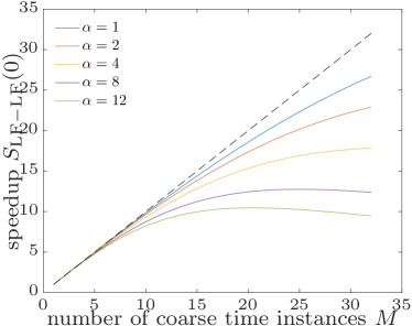
(a) Local-forecast initialization

(b) Global-forecast initialization

Fig. 3: Ideal-conditions speedup. Plot corresponds to $m=5000$ fine time instances, setting the number of processors equal to the number of coarse time instances ${M}$.

To illustrate the full potential of the proposed approach, Appendix B demonstrates that super-ideal speedups can be realized when the proposed methodology is combined with the method presented in Ref. [12] for defining Newton-solver initial guesses via forecasting.

4.3 Stability analysis

We begin by providing a general proof for stability of the parareal recurrence; we then derive specific quantities needed to demonstrate stability when the proposed forecast is employed as a coarse propagator. These results employ a subset of the following assumptions:

1. The fine propagator is stable, i.e., $\|\mathcal{F}({\boldsymbol{\xi}};{{t}^{i}},{{t}^{j}})\|\leq(1+C_{\mathcal{F}}({{t}^{j}}-{{t}^{i}}))\|{\boldsymbol{\xi}}\|,\ \forall{\boldsymbol{\xi}}\in\mathbb{R}^{N}.$

2. The restriction operators and prolongation operator counterparts are bounded by constants $M_{\perp}$, $M_{{\mathbf{r}_{j}}}\in\mathbb{R}$, i.e., $\|{\mathbf{P}_{\perp}}{\mathbf{R}^{T}_{\perp}}{\boldsymbol{\xi}}\|\leq M_{\perp}\|{\boldsymbol{\xi}}\|,\ \forall{\boldsymbol{\xi}}\in\mathbb{R}^{N}$ and $\|{\mathbf{r}^{T}_{j}}{\boldsymbol{\xi}}\|\leq M_{{\mathbf{r}_{j}}}\|{\boldsymbol{\xi}}\|,\ \forall{\boldsymbol{\xi}}\in\mathbb{R}^{N}$.

The following lemma follows some elements of the stability analysis performed in Ref. [14].

Lemma 8 (General parareal stability).

If constants $\alpha_{A}$ and $C_{A}$ exist such that the coarse propagator can be bounded as

(25) $$\|\mathcal{G}({\boldsymbol{\xi}};{T}^{{{n}}},{T}^{{{n}}+1})\|\leq\alpha_{A}(1+C_{A}{H})\|{\boldsymbol{\xi}}\|$$

and constants $\alpha_{B}$ and $C_{B}$ exist such that the difference between the coarse and fine propagators can be bounded as

(26) $$\|\mathcal{F}({\boldsymbol{\xi}};{T}^{{{n}}},{T}^{{{n}}+1})-\mathcal{G}({\boldsymbol{\xi}};{T}^{{{n}}},{T}^{{{n}}+1})\|\leq\alpha_{B}(1+C_{B}{H})\|{\boldsymbol{\xi}}\|,$$

then the parareal recurrence (4) is stable, as it satisfies

(27) $$\quad\quad\|{\mathbf{x}}^{{{{n}}}}_{{k}}\|\leq (\alpha_{A})^{{n}}\exp(C_{A}{{n}}H)\|{\mathbf{x}}^{0}\|\!+\!\sum_{j=1}^{{n}}(\alpha_{A})^{{{n}}-j}\alpha_{B}\exp((({{n}}-j)C_{A}\!+\!C_{B})H)\|{\mathbf{x}}^{j-1}_{{k}-1}\|,\ {{n}}\!\in{\rm Nature}{{M}},{k}\!\in{\rm Nature}{{{n}}}$$

(28) $$\|{\mathbf{x}}^{{{{n}}}}_{{k}}\|\leq \sum_{j=0}^{{{{n}}}}{{{{n}}}\choose j}(\alpha_{A})^{j}(\alpha_{B})^{{{{n}}}-j}\exp\left(\left(jC_{A}+({{n}}-j)C_{B}\right)H\right)\|{\mathbf{x}}^{0}\|,\quad{{n}}\in{\rm Nature}{{M}},\ {k}={{n}}.$$

We now derive the quantities $\alpha_{A}$, $C_{A}$, $\alpha_{B}$, and $C_{B}$ from Lemma 8 that are specific to the proposed coarse propagator ${\mathcal{G}_{\mathrm{LF}}}$.

Lemma 9 (Stability of proposed coarse propagator).

Under Assumptions A2, A9, and A10

(29) $$\|{\mathcal{G}_{\mathrm{LF}}}({\boldsymbol{\xi}};{T}^{{{{n}}}},{T}^{{{{n}}}+1})\|\leq\sqrt{{\bar{N}}}M_{\mathbf{P}}\max_{j\in{\rm Nature}{{\bar{N}}}}M_{{\mathbf{r}_{j}}}\alpha_{j}^{n}\left(1+C_{j}^{n}C_{\mathcal{F}}H\right)\|{\boldsymbol{\xi}}\|,$$

where we have defined $\alpha_{j}^{n}\vcentcolon=\left(\lambda_{j}^{{{n}}}+\kappa_{j}^{{{n}}}\sqrt{\alpha}\right)\geq 1$, $C_{j}^{n}\vcentcolon=\frac{(\alpha/{\bar{m}})\kappa_{j}^{{{n}}}\sqrt{\alpha}}{\lambda_{j}^{{{n}}}+\kappa_{j}^{{{n}}}\sqrt{\alpha}}\leq 1$, $\lambda_{j}^{{{n}}}\vcentcolon=|1-\sum_{i=1}^{\alpha}{\gamma}_{ij}^{{n}}|$ and $\kappa_{j}^{{{n}}}\vcentcolon=\sqrt{\sum_{i=1}^{\alpha}({\gamma}_{ij}^{{n}})^{2}}$. Hence, we have proven stability in the sense of Eq. (25).

Remark 4.5 (Bound dependence on discretization).

For a fixed coarse time step $H$ and time-sampling fraction $\alpha/{\bar{m}}$, the only quantities in bound (29) that depend on the underlying (fine) time discretization (i.e., $h$, ${\bar{m}}$) are the stability constants $\alpha_{j}^{n}$ and $C_{j}^{n}$. We now assess the dependence of these stability constants on the time discretization. For a fixed sampling time interval, the stability constants $\alpha_{j}^{n}$ and $C_{j}^{n}$ approach constant values as the time step approaches zero. This can be seen from the scaling of the terms that compose the constant as the (fine) time step $h$ decreases: $\sqrt{\alpha}$ increases with an exponential power of 1/2, $\kappa_{j}^{{{n}}}$ decreases with an exponential power of 1/2, and $\lambda_{j}^{{{n}}}$ is constant. The second of these trends arises from the fact that the columns of the matrix $\mathbf{\Xi}_{j}^{{n}}\in\mathbb{V}_{{a}}(\mathbb{R}^{{\bar{m}}})$ remain orthogonal when the fine time step $h$ changes. Figure 4 reports a numerical investigation of these trends.

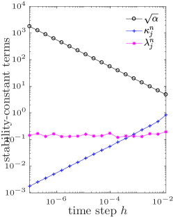
(a) scaling of terms in stability constant

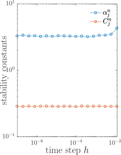
(b) scaling of the stability constants

Fig. 4: Scaling of the stability constants in bound (29). Data correspond to a coarse time interval ${H}=1$, a time-sampling fraction of $\alpha/{\bar{m}}=0.3$; reported values correspond to averages taken over 50 random orthogonal matrices $\mathbf{\Xi}_{j}^{{n}}$. Note that the stability constants approach constant values as the fine time step decreases, which implies that bound (29) is independent of the time discretization for sufficiently small time steps.

Remark 4.6 (Superior stability of global-forecasting initialization to local-forecasting initialization).

We now consider the implications of Lemma 9 in terms of the two initialization methods proposed in Section 3.4. The first proposal involved applying the local forecast for initialization, i.e., computing the initial values ${\mathbf{x}}^{{{n}}}_{0}$, ${{n}}\in{\rm Nature}{{M}}$ via Eq. (17) with $\mathcal{G}\leftarrow{\mathcal{G}_{\mathrm{LF}}}$. Applying inequality (29) to Eq. (17) with $\mathcal{G}\leftarrow{\mathcal{G}_{\mathrm{LF}}}$ leads to the following stability result for the computed initial values: $\|{\mathbf{x}}^{{{n}}}_{0}\|\leq({\upsilon})^{{n}}\|{\mathbf{x}}^{0}\|,\ {{n}}\in{\rm Nature}{{M}}.$ Here, ${\upsilon}\vcentcolon=\sqrt{{\bar{N}}}M_{\mathbf{P}}\max_{j\in{\rm Nature}{{\bar{N}}},n\in\mathbb{N}_{0}({M}-1)}M_{{\mathbf{r}_{j}}}\alpha_{j}^{n}\left(1+C_{j}^{n}C_{\mathcal{F}}H\right)$; that is, the stability factor associated with local-forecast initialization grows exponentially in the number of coarse time instances ${{n}}$. This phenomenon can be interpreted as follows: small errors in a local forecast can be amplified by subsequent local forecasts, as these are performed sequentially.

On the other hand, by comparing Eqs. (18) and (15), one can note that global-forecast initialization (18) is equivalent to applying the local forecast with global time-evolution bases $\mathbf{\Xi}_{j}$ over a time interval ${T}^{{{n}}+1}-{T}^{0}$. Thus, the stability of the global-forecast initialization can be derived directly from inequality (29) applied with these modifications as

(30) $$\|{\mathbf{x}}^{{{n}}+1}_{0}\|\leq\bar{\upsilon}\|{\mathbf{x}}^{0}\|,\quad{{n}}\in\mathbb{N}_{0}({M}-1).$$

Here, we have defined

$$\bar{\upsilon}\vcentcolon=\sqrt{{\bar{N}}}M_{\mathbf{P}}\max_{j\in{\rm Nature}{{\bar{N}}},n\in\mathbb{N}_{0}({M}-1)}M_{{\mathbf{r}_{j}}}\bar{\alpha}_{j}^{n}\left(1+\bar{C}_{j}^{n}C_{\mathcal{F}}H\right),$$

$\bar{\alpha}_{j}^{n}\vcentcolon=\left(\bar{\lambda}_{j}^{{{n}}}+\bar{\kappa}_{j}^{{{n}}}\sqrt{\alpha}\right)\geq 1$, $\bar{C}_{j}^{n}\vcentcolon=\frac{(\alpha/{\bar{m}})\bar{\kappa}_{j}^{{{n}}}\sqrt{\alpha}}{\bar{\lambda}_{j}^{{{n}}}+\bar{\kappa}_{j}^{{{n}}}\sqrt{\alpha}}\leq 1$, $\bar{\lambda}_{j}^{{{n}}}\vcentcolon=|1-\sum_{i=1}^{\alpha}{\bar{\gamma}}_{ij}^{{{n}}}|$, and $\bar{\kappa}_{j}^{{{n}}}\vcentcolon=\sqrt{\sum_{i=1}^{\alpha}({\bar{\gamma}}_{ij}^{{{n}}})^{2}}$. Inequality (30) shows that the stability factor associated with global-forecast initialization does not grow with the number of coarse time instances; it depends on the coarse time instance only through the quantities $\bar{\lambda}_{j}^{{{n}}}$ and $\bar{\kappa}_{j}^{{{n}}}$, which should not grow with ${{n}}$. This phenomenon can be interpreted as follows: small forecasting errors cannot be amplified, as a single forecast is employed for the entire time interval.

Lemma 10 (Stability of difference between fine and proposed coarse propagators).

If Assumptions A1, A2, A9, and A10 hold, then

(31) $$\begin{split}\|\mathcal{F}({\boldsymbol{\xi}};{T}^{{{n}}},{T}^{{{n}}+1})-{\mathcal{G}_{\mathrm{LF}}}({\boldsymbol{\xi}};{T}^{{{n}}},{T}^{{{n}}+1})\|\leq(M_{\perp}+\sqrt{{\bar{N}}}M_{\mathbf{P}}\max_{j\in{\rm Nature}{{\bar{N}}}}M_{{\mathbf{r}_{j}}}(\alpha_{j}^{n}+1))\left(1+C_{\mathcal{F}}H\right)\|{\boldsymbol{\xi}}\|.\end{split}$$

Theorem 11 (Parareal stability with proposed coarse propagator).

Under Assumptions A1, A2, A9, and A10, employing the proposed coarse propagator in the parareal recurrence (i.e., $\mathcal{G}\leftarrow{\mathcal{G}_{\mathrm{LF}}}$ in Eq. (4)) yields a stable recurrence, as the iterates satisfy Eqs. (27) and (28) with

(32) $$\alpha_{A}=\sqrt{{\bar{N}}}M_{\mathbf{P}}\max_{j\in{\rm Nature}{{\bar{N}}},n\in\mathbb{N}_{0}({M}-1)}M_{{\mathbf{r}_{j}}}\alpha_{j}^{n},\quad C_{A}=C_{\mathcal{F}}\max_{j\in{\rm Nature}{{\bar{N}}},n\in\mathbb{N}_{0}({M}-1)}C_{j}^{n},$$

(33) $$\alpha_{B}=(M_{\perp}+\sqrt{{\bar{N}}}M_{\mathbf{P}}\max_{j\in{\rm Nature}{{\bar{N}}}}M_{{\mathbf{r}_{j}}}(\alpha_{j}^{n}+1)),\quad C_{B}=C_{\mathcal{F}}.$$

Remark 4.5 shows that, for a fixed coarse time step $H$ and time-sampling fraction $\alpha/{\bar{m}}$, the stability constants $\alpha_{j}^{n}$ and $C_{j}^{n}$ approach constant values as the time step $h$ approaches zero. As all other quantities in the stability bounds (27)–(28) (with coefficients specified in Theorem 11) are independent of the underlying fine time discretization (i.e., $h$ and ${\bar{m}}$), we know the stability result is not sensitive to the selected fine time step if it is taken to be sufficiently small.

4.4 Convergence analysis

Recall that the proposed approach merely defines alternative techniques for initialization and coarse propagation for the parareal method. Thus, one might expect that existing convergence results derived for the parareal methods still hold in the present context. However, this is not always the case, as many existing results assume that the coarse propagator corresponds to a time integrator with a known order of accuracy [33, 3, 4, 28]; the local-forecast coarse propagator cannot be straightforwardly assigned such an order of accuracy, as its error is bounded by an expression that does not explicitly depend on the coarse time step $H$ (see Theorem 1).

Instead, we can make use of existing convergence results that require only a general definition of the coarse propagator. One such example is the convergence analysis of Ref. [29], which assumes a fixed coarse time step $H$ and assesses convergence as the number of parareal iterations increases. We proceed by describing how the proposed initialization and coarse propagator affect these convergence results.

Following Ref. [29], we now consider a simplified problem setting that relies on the following assumptions:

1. Problem (1) is scalar and linear i.e., $N=1$ and $g:({\xi};t)\mapsto a{\xi}$ with $a\in\mathbb{R}$.

2. The coarse propagator is a linear operator, i.e., $\mathcal{G}:({\xi};{T}^{i},{T}^{j})\mapsto(\bar{a}_{\mathcal{G}})^{j-i}{\xi}$ with $\bar{a}_{\mathcal{G}}\in\mathbb{R}$.

3. The coarse propagator is in its region of absolute stability such that $|\bar{a}_{\mathcal{G}}|<1$.

We note that under Assumption A11, problem (1) simplifies to

(34) $$\frac{d}{dt}{x^{\star}}(t) =ax^{\star},\quad x^{\star}(0)=x^{0}\ ,$$

where $x^{\star}:\mathbb{R}_{+}\rightarrow\mathbb{R}$ and the fine propagator becomes a linear operator satisfying $\mathcal{F}:({\xi};{{t}^{i}},{{t}^{j}})\mapsto(\bar{a}_{\mathcal{F}})^{j-i}{\xi}$ with $\bar{a}_{\mathcal{F}}\in\mathbb{R}$. For example, the backward-Euler fine propagator becomes $\mathcal{F}_{\mathrm{BE}}:({\xi};{{t}^{i}},{{t}^{j}})\mapsto(\bar{a}_{\text{BE}})^{j-i}{\xi}$ with $\bar{a}_{\text{BE}}\vcentcolon=(1-ha)^{-1}$. Theorem 4.5 (with Corollary 4.6) of that reference is repeated below (including modifications discussed in Section 4.5 of Ref. [29]) in the current notation.

Theorem 12 (Parareal convergence (Theorem 4.5 and Corollary 4.6 of [29])).

If $T_{\mathrm{final}}<\infty$ and Assumptions A11 and A12 hold, then

(35) $$\max_{n\in{\rm Nature}{{M}}}|x({T}^{n})-x^{n}_{k}|\leq|(\bar{a}_{\mathcal{F}})^{\bar{m}}-\bar{a}_{\mathcal{G}}|^{k}\|(\mathbf{M}(\bar{a}_{\mathcal{G}}))^{k}\|_{\infty}\max_{n\in{\rm Nature}{{M}}}|x({T}^{n})-x^{n}_{0}|,$$

where $\mathbf{M}\in\mathbb{R}^{{M}\times{M}}$ is a Toeplitz matrix whose elements are defined by the value of the elements in the first column, which are

(36) $$m_{i,1}(\beta)=\begin{cases}0,\quad&i=1\\ \beta^{i-2},\quad&i\in\{2,\ldots,{M}\}\end{cases}$$

If additionally Assumption A13 holds, the recurrence converges superlinearly as

(37) $$\max_{n\in{\rm Nature}{{M}}}|x({T}^{n})-x^{n}_{k}|\leq\frac{|(\bar{a}_{\mathcal{F}})^{\bar{m}}-\bar{a}_{\mathcal{G}}|^{k}\prod_{j=1}^{k}({M}-j)}{k!}\max_{n\in{\rm Nature}{{M}}}|x({T}^{n})-x^{n}_{0}|.$$

We now describe how our prescribed coarse propagator can be integrated in this convergence result. First, we note that under Assumption A11, the proposed coarse propagator is characterized by ${\mathbf{R}}={\mathbf{P}}=1$ and ${\bar{N}}=N=1$. We now collect assumptions related to the proposed coarse propagator:

1. The same local basis is employed for every coarse time interval, i.e., $\mathbf{\Xi}^{i}=\mathbf{\Xi}^{j}=\mathbf{\Xi}\in\mathbb{V}_{{a}}(\mathbb{R}^{{\bar{m}}})$, $i,j\in\mathbb{N}_{0}({M}-1)$.

2. The forecast satisfies the inequality $|1+\sum_{i=1}^{\alpha}{\gamma}_{i}[(\bar{a}_{\mathcal{F}})^{i}-1]|<1$ with ${\gamma}_{i}\vcentcolon=\mathbf{e}_{{\bar{m}}}^{T}\mathbf{\Xi}\left[{{\mathbf{Z}}_{0}}\mathbf{\Xi}\right]^{+}\mathbf{e}_{i}\in\mathbb{R}$, $i\in{\rm Nature}{\alpha}$.

We now show that the parareal recurrence executed with the proposed coarse propagator converges superlinearly under the stated conditions.

Corollary 13 (Superlinear parareal convergence using the proposed coarse propagator).

Under Assumptions A11 and A14, the proposed coarse propagator is linear and satisfies ${\mathcal{G}_{\mathrm{LF}}}:({\xi};{T}^{{{n}}},{T}^{{{n}}+1})\mapsto\bar{a}_{\text{LF}}{\xi}$ with $\bar{a}_{\text{LF}}\vcentcolon=1+\sum_{i=1}^{\alpha}{\gamma}_{i}[(\bar{a}_{\mathcal{F}})^{i}-1]$. Further, the error in the parareal recurrence executed with the proposed coarse propagator $\mathcal{G}\leftarrow{\mathcal{G}_{\mathrm{LF}}}$ satisfies

(38) $$\max_{n\in{\rm Nature}{{M}}}|x({T}^{n})-x^{n}_{k}| \leq(\rho)^{k}\|(\mathbf{M}(\bar{a}_{\text{LF}}))^{k}\|_{\infty}\max_{n\in{\rm Nature}{{M}}}|x({T}^{n})-x^{n}_{0}|.$$

where $\rho\vcentcolon=|(\bar{a}_{\mathcal{F}})^{\bar{m}}-\bar{a}_{\text{LF}}|=|(\bar{a}_{\mathcal{F}})^{\bar{m}}-1-\sum_{i=1}^{\alpha}{\gamma}_{i}[(\bar{a}_{\mathcal{F}})^{i}-1]|$. If Assumption A15 additionally holds, then the recurrence converges superlinearly as

(39) $$\max_{n\in{\rm Nature}{{M}}}|x({T}^{n})-x^{n}_{k}| \leq\frac{(\rho)^{k}\left(\prod_{j=1}^{k}({M}-j)\right)}{k!}\max_{n\in{\rm Nature}{{M}}}|x({T}^{n})-x^{n}_{0}|.$$

Remark 4.7 (Role of accuracy in convergence).

Inequalities (38)–(39) demonstrate the effect of coarse-propagation and initial-seed accuracy on convergence. In particular, the term $\rho$ represents the error the coarse propagator incurs with respect to the fine propagator; this is precisely the quantity we aim to minimize with the proposed coarse propagator. In fact, Theorem 1 bounds this error, and Theorem 3 demonstrates that this error is zero under ‘ideal conditions’. Further, the error incurred by the initial seed appears as $\max_{n\in{\rm Nature}{{M}}}|x({T}^{n})-x^{n}_{0}|$ in these results. This is the term we aim to minimize by applying the proposed local and global forecasting methods for initialization; this quantity is also zero under the ‘ideal conditions’ stated in Theorem 3.

5 Computing forecasting ingredients via SVD/POD

We now describe how the three ingredients that define the proposed methodology—the time-evolution bases $\mathbf{\Xi}_{j}$, $j\in{\rm Nature}{N}$, the restriction operator ${\mathbf{R}}$, and the prolongation operator ${\mathbf{P}}$—can be computed using the POD method. Section 5.1 describes this for the case of parameterized ODEs, while Section 5.2 specializes this for the case of POD-based ROMs.

5.1 Parameterized ODEs

We first introduce a parameterized variant of the governing initial-value ordinary-differential-equation (ODE) problem (1).

(40) $$\frac{d}{dt}{\mathbf{x}^{\star}}(t,\boldsymbol{\mu})={\mathbf{g}}\left(\mathbf{x}^{\star};t,\boldsymbol{\mu}\right),\quad\mathbf{x}^{\star}(0,\boldsymbol{\mu})=\mathbf{x}^{0}(\boldsymbol{\mu})\ ,$$

where $\boldsymbol{\mu}\in\mathcal{D}\subset\mathbb{R}^{p}$ denotes the parameters, $\mathbf{x}^{\star}:\mathbb{R}_{+}\times\mathcal{D}\rightarrow\mathbb{R}^{N}$ denotes the (parameterized) state implicitly defined as the exact solution to problem (40), ${\mathbf{g}}:\mathbb{R}^{N}\times\mathbb{R}_{+}\times\mathcal{D}\rightarrow\mathbb{R}^{N}$ with $({\boldsymbol{\xi}};{t},{\boldsymbol{\nu}})\mapsto{\mathbf{g}}({\boldsymbol{\xi}};{t},{\boldsymbol{\nu}})$ denotes the velocity, and $\mathbf{x}^{0}:\mathcal{D}\rightarrow\mathbb{R}^{N}$ denotes the initial state. Analogously to Eq. (3), we define $\mathbf{x}(\cdot,\boldsymbol{\mu}):{t}\mapsto\mathcal{F}(\mathbf{x}^{0}(\boldsymbol{\mu});0,{t})$ for ${t}\in\mathcal{t}$ as the associated numerical solution with $\mathbf{x}(\cdot,\boldsymbol{\mu})\in(\mathcal{H})^{N}$.

Algorithm 5 pod

0:  training parameter instances $\{\bar{\boldsymbol{\mu}}_{i}\}_{i=1}^{N_{\text{train}}}\subset\mathcal{D}$, $\upsilon\in\left[0,1\right]$

0:  POD state basis $\mathbf{U}\in\mathbb{V}_{q}(\mathbb{R}^{N})$, POD time-evolution bases $\mathbf{V}_{j}\in\mathbb{V}_{N_{\text{train}}}(\mathbb{R}^{m})$, $j=1,\ldots,q$

1:  for $i=1,\ldots,N_{\text{train}}$ do {collect snapshots}

2:     Numerically solve Eq. (40) with $\boldsymbol{\mu}\leftarrow\bar{\boldsymbol{\mu}}_{i}$ to obtain snapshots $\mathbf{X}_{i}\vcentcolon=[\mathbf{x}(t^{1},\bar{\boldsymbol{\mu}}_{i})-\mathbf{x}^{0}(\bar{\boldsymbol{\mu}}_{i})\ \cdots\ \mathbf{x}(t^{m},\bar{\boldsymbol{\mu}}_{i})-\mathbf{x}^{0}(\bar{\boldsymbol{\mu}}_{i})]\in\mathbb{R}^{N\times m}$

3:  end for

4:   $(\mathbf{U},\mathbf{\Sigma},\mathbf{V})=\texttt{thin\_SVD}(\left[\mathbf{X}_{1}\ \cdots\ \mathbf{X}_{N_{\text{train}}}\right])$ {Compute (thin) singular value decomposition}

5:   $\mathbf{U}\leftarrow\begin{bmatrix}\mathbf{u}_{1}\ \cdots\ \mathbf{u}_{q}\end{bmatrix}$, where $q=\min_{i\in\Upsilon(\upsilon)}i$, $\Upsilon(\upsilon)\vcentcolon=\{i\ |\ \sum_{j=1}^{i}\sigma_{j}/\sum_{k=1}^{mN_{\text{train}}}\sigma_{k}\geq\upsilon\}$, $\mathbf{\Sigma}=\mathrm{diag}(\sigma_{1},\ldots,\sigma_{mN_{\text{train}}})$. {Compute truncated state basis}

6:  for $j=1,\ldots,q$ do {Extract temporal bases from right singular vectors}

7:     $(\mathbf{Q}_{j},\mathbf{R}_{j})=\texttt{thin\_QR}([\mathbf{v}_{j}^{1}\ \cdots\ \mathbf{v}_{j}^{N_{\text{train}}}])$ with $\mathbf{v}_{j}^{i}\vcentcolon=[v_{j,m(i-1)+1}\ \cdots\ v_{j,mi}]^{T}$ {Compute (thin) QR factorization}

8:     $\mathbf{V}_{j}\leftarrow\mathbf{Q}_{j}$

9:  end for

The ingredients required for the proposed methodology can be computed in a data-driven manner via the POD method by executing the following steps:

1. Given training parameter instances $\{\bar{\boldsymbol{\mu}}_{i}\}_{i=1}^{N_{\text{train}}}\subset\mathcal{D}$ and energy criterion $\upsilon\in[0,1]$, execute Algorithm 5 to obtain POD state basis $\mathbf{U}\in\mathbb{V}_{q}(\mathbb{R}^{N})$ and POD time-evolution bases $\mathbf{V}_{j}\in\mathbb{V}_{N_{\text{train}}}(\mathbb{R}^{m})$, $j\in{\rm Nature}{q}$.

2. Set the forecasting time-evolution bases equal to the POD time-evolution bases $\mathbf{\Xi}_{j}\leftarrow\mathbf{V}_{j}$, $j\in{\rm Nature}{q}$. Note that ${\bar{N}}=q$ and ${a}=N_{\text{train}}$.

3. Define the restriction and prolongation operators as ${\mathbf{R}}\leftarrow\mathbf{U}$ and ${\mathbf{P}}\leftarrow\mathbf{U}$, respectively.

This approach is sensible, as numerous studies have shown that POD tends to truncate solution modes associated with high-frequency temporal behavior [9]. Thus, the resulting restriction operator will ensure that forecasting is applied only to the long-temporal-wavelength solution components. We note that this approach is equivalent to computing ‘tailored’ temporal subspaces [15] via the sequentially truncated high-order SVD [49].

Remark 5.1 (Ideal predictive case for parameterized linear ODEs).

For illustration, consider a variant of the initial-value ODE problem (40) wherein the velocity is linear in the state but independent of time and the parameters, i.e., ${\mathbf{g}}:({\boldsymbol{\xi}};{t},{\boldsymbol{\nu}})\mapsto\mathbf{A}{\boldsymbol{\xi}}$, the initial condition exhibits separable parameter dependence, i.e., $\mathbf{x}^{0}(\boldsymbol{\mu})=\sum_{i=1}^{r}\Theta^{i}(\boldsymbol{\mu})\bar{\mathbf{x}}^{i}$ with $\Theta^{i}:\mathcal{D}\rightarrow\mathbb{R}$ and $\bar{\mathbf{x}}^{i}\in\mathbb{R}^{N}$, $i\in{\rm Nature}{r}$ linearly independent, and the parameter set is unbounded, i.e., $\mathcal{D}=\mathbb{R}^{p}$. Then, problem (40) becomes

(41) $$\frac{d}{dt}{\mathbf{x}^{\star}}(t,\boldsymbol{\mu})=\mathbf{A}\mathbf{x}^{\star}(t,\boldsymbol{\mu}),\quad\mathbf{x}^{\star}(0,\boldsymbol{\mu})=\sum_{i=1}^{r}\Theta^{i}(\boldsymbol{\mu})\bar{\mathbf{x}}^{i}.$$

In this case, the fine propagator is also linear and can be written as $\mathcal{F}:({\boldsymbol{\xi}};{{t}^{i}},{{t}^{j}})\mapsto(\bar{\mathbf{A}}_{\mathcal{F}})^{j-i}{\boldsymbol{\xi}}$. For example, the backward-Euler fine propagator becomes $\mathcal{F}_{\mathrm{BE}}:({\boldsymbol{\xi}};{{t}^{i}},{{t}^{j}})\mapsto(\bar{\mathbf{A}}_{\text{BE}})^{j-i}{\boldsymbol{\xi}}$ with $\bar{\mathbf{A}}_{\text{BE}}\vcentcolon=(\mathbf{I}_{N}-h\mathbf{A})^{-1}$. Therefore, the discrete solution is simply

(42) $${\mathbf{x}}(t^{j},\boldsymbol{\mu}) =\mathcal{F}(\mathbf{x}(0,\boldsymbol{\mu});0,{{t}^{j}})=(\bar{\mathbf{A}}_{\mathcal{F}})^{j}\mathbf{x}(0,\boldsymbol{\mu})=(\bar{\mathbf{A}}_{\mathcal{F}})^{j}\sum_{i=1}^{r}\Theta^{i}(\boldsymbol{\mu})\bar{\mathbf{x}}^{i},\quad j\in\mathbb{N}_{0}(m)$$

Now, assume that $N_{\text{train}}=r$ training parameter instances $\{\bar{\boldsymbol{\mu}}_{i}\}_{i=1}^{r}$ are employed such that the matrix $\mathbf{D}\in\mathbb{R}^{r\times r}$ with elements $d_{ij}\vcentcolon=\Theta^{i}(\bar{\boldsymbol{\mu}}_{j})$ is invertible. Then, we have $\left[\bar{\mathbf{x}}^{1}\ \cdots\ \bar{\mathbf{x}}^{r}\right]=\left[\mathbf{x}(0,\bar{\boldsymbol{\mu}}_{1})\ \cdots\ \mathbf{x}(0,\bar{\boldsymbol{\mu}}_{r})\right]\mathbf{D}^{-1}$ and Eq. (42) becomes

(43) $${\mathbf{x}}(t^{j},\boldsymbol{\mu}) =(\bar{\mathbf{A}}_{\mathcal{F}})^{j}\sum_{i=1}^{r}\bar{\Theta}^{i}(\boldsymbol{\mu})\mathbf{x}(0,\bar{\boldsymbol{\mu}}_{i})=\sum_{i=1}^{r}\bar{\Theta}^{i}(\boldsymbol{\mu})(\bar{\mathbf{A}}_{\mathcal{F}})^{j}\mathbf{x}(0,\bar{\boldsymbol{\mu}}_{i})=\sum_{i=1}^{r}\bar{\Theta}^{i}(\boldsymbol{\mu})\mathbf{x}({{t}^{j}},\bar{\boldsymbol{\mu}}_{i}),\quad j\in\mathbb{N}_{0}(m)$$

where $\bar{\Theta}^{i}(\boldsymbol{\mu})\vcentcolon=\sum_{j=1}^{r}[\mathbf{D}^{-1}]_{ij}\Theta^{j}(\boldsymbol{\mu})$. Therefore, we have ${\mathbf{x}}(t^{j},\boldsymbol{\mu})-{\mathbf{x}}(0,\boldsymbol{\mu})=\sum_{i=1}^{r}\bar{\Theta}^{i}(\boldsymbol{\mu})(\mathbf{x}({{t}^{j}},\bar{\boldsymbol{\mu}}_{i})-\mathbf{x}(0,\bar{\boldsymbol{\mu}}_{i})),$ or equivalently

(44) $${\mathbf{h}}({x}_{j}(\cdot,\boldsymbol{\mu}))\in\mathrm{Ran}(\left[{\mathbf{h}}({x}_{j}(\cdot,\bar{\boldsymbol{\mu}}_{1}))\ \cdots\ {\mathbf{h}}({x}_{j}(\cdot,\bar{\boldsymbol{\mu}}_{r}))\right]),\quad j\in{\rm Nature}{N},\ \forall\boldsymbol{\mu}\in\mathcal{D}.$$

Thus, employing ${\mathbf{R}}={\mathbf{P}}=\mathbf{I}_{N}$ (such that ${\bar{N}}=N$) with $\mathbf{\Xi}_{j}=\left[{\mathbf{h}}({x}_{j}(\cdot,\bar{\boldsymbol{\mu}}_{1}))\ \cdots\ {\mathbf{h}}({x}_{j}(\cdot,\bar{\boldsymbol{\mu}}_{r}))\right]$, $j\in{\rm Nature}{{\bar{N}}}$ in this case ensures that Assumptions A3 and A5 hold. Then, if the local bases are constructed with no truncation (i.e., Assumption A4 holds), the coarse propagator is exact (see Theorem 3). Further, the proposed method converges in ${K}=0$ iterations if initialization is computed either via local forecasting (i.e., Assumption A6 holds; see Theorem 6) or via global forecasting (i.e., Assumption A7 holds; see Theorem 7). So this is an example where the forecast of the proposed method is equivalent to the fine propagator for all parameters $\boldsymbol{\mu}\in\mathbb{R}^{p}$; hence, it is an ideal predictive coarse propagator.

5.2 POD-based reduced-order model

Projection-based model reduction aims to reduce the cost of numerically solving Eq. (40) by reducing the dimensionality of the governing equations. To achieve this, these techniques employ a ‘trial basis’ $\mathbf{\Phi}\in\mathbb{R}_{\star}^{N\times{\hat{N}}}$ with reduced state dimension ${\hat{N}}\leq N$, and subsequently approximate the state as ${\tilde{\mathbf{x}}}^{\star}:(t,{\boldsymbol{\nu}})\mapsto\mathbf{x}^{0}(\boldsymbol{\mu})+\mathbf{\Phi}{\hat{\mathbf{x}}}^{\star}(t,{\boldsymbol{\nu}})$. Here, $\mathbb{R}_{\star}^{m\times n}$ denotes the set of full-column-rank $m\times n$ real-valued matrices (i.e., the noncompact Stiefel manifold), and the reduced state ${\hat{\mathbf{x}}}^{\star}:\mathbb{R}_{+}\times\mathbb{R}^{p}\rightarrow\mathbb{R}^{{\hat{N}}}$ satisfies

(45) $$\frac{d}{dt}{\hat{\mathbf{x}}}^{\star}(t,\boldsymbol{\mu})=\hat{\mathbf{g}}\left({\hat{\mathbf{x}}}^{\star};t,\boldsymbol{\mu}\right),\quad{\hat{\mathbf{x}}}^{\star}(0,\boldsymbol{\mu})={{\mathbf{0}}},$$

where $\hat{\mathbf{g}}:(\hat{\boldsymbol{\xi}};{t},{\boldsymbol{\nu}})\mapsto(\mathbf{\Psi}(\hat{\boldsymbol{\xi}};{t},{\boldsymbol{\nu}})^{T}\mathbf{\Phi})^{-1}\mathbf{\Psi}(\hat{\boldsymbol{\xi}};{t},{\boldsymbol{\nu}})^{T}{\mathbf{g}}\left(\mathbf{x}^{0}({\boldsymbol{\nu}})+\mathbf{\Phi}\hat{\boldsymbol{\xi}};{t},{\boldsymbol{\nu}}\right)$ denotes the reduced velocity and $\mathbf{\Psi}:\mathbb{R}^{{\hat{N}}}\times\mathbb{R}_{+}{}\times\mathbb{R}^{p}\rightarrow\mathbb{R}_{\star}^{N\times{\hat{N}}}$ denotes the ‘test basis’. Note that Eq. (45) enforces the ODE residual $\frac{d}{dt}{\tilde{\mathbf{x}}}^{\star}(t,\boldsymbol{\mu})-{\mathbf{g}}\left({\tilde{\mathbf{x}}}^{\star}(t,\boldsymbol{\mu});t,\boldsymbol{\mu}\right)$ to be orthogonal to $\mathrm{Ran}(\mathbf{\Psi}\left(\hat{\mathbf{x}};t,\boldsymbol{\mu}\right))$. The test basis can be set equal to the trial basis (i.e., $\mathbf{\Psi}\left(\hat{\mathbf{x}};t,\boldsymbol{\mu}\right)=\mathbf{\Phi}$)—which is referred to as Galerkin projection—or can be chosen to minimize the discrete residual arising after time discretization (e.g., $\mathbf{\Psi}\left(\hat{\mathbf{x}};t,\boldsymbol{\mu}\right)=[\alpha_{0}\mathbf{I}-h\beta_{0}\partial{\mathbf{g}}/\partial{\boldsymbol{\xi}}(\mathbf{x}^{0}+\mathbf{\Phi}\hat{\mathbf{x}};t,\boldsymbol{\mu})]\mathbf{\Phi}$ for linear multistep schemes, where $\alpha_{0}$ and $\beta_{0}$ are coefficients for a given scheme), which is referred to as least-squares Petrov–Galerkin projection [10, 11, 9], for example. Again, we define $\hat{\mathbf{x}}(\cdot,\boldsymbol{\mu}):{t}\mapsto\mathcal{F}(\hat{\mathbf{x}}^{0}(\boldsymbol{\mu});0,{t}),$ as the associated numerical solution with $\hat{\mathbf{x}}(\cdot,\boldsymbol{\mu})\in(\mathcal{H})^{\hat{N}}$.

When the trial basis $\mathbf{\Phi}$ is computed via POD, both the trial basis and the proposed method’s ingredients can be computed by executing the following steps:

1. Given training parameter instances $\{\bar{\boldsymbol{\mu}}_{i}\}_{i=1}^{N_{\text{train}}}\subset\mathcal{D}$ and energy criterion $\upsilon\in[0,1]$, execute Algorithm 5 to obtain POD state basis $\mathbf{U}\in\mathbb{V}_{q}(\mathbb{R}^{N})$ and POD time-evolution bases $\mathbf{V}_{j}\in\mathbb{V}_{N_{\text{train}}}(\mathbb{R}^{m})$, $j\in{\rm Nature}{q}$.

2. Set the trial basis equal to the POD state basis $\mathbf{\Phi}\leftarrow\mathbf{U}$; note that ${\hat{N}}=q$.

3. Set the forecasting time-evolution bases equal to the truncated POD time evolution bases such that only the first ${\bar{N}}$ (with ${\bar{N}}\leq q={\hat{N}}$) POD modes are employed for forecasting: $\mathbf{\Xi}_{j}\leftarrow\mathbf{V}_{j}$, $j\in{\rm Nature}{{\bar{N}}}$. Note that ${a}=N_{\text{train}}$.

4. Define the restriction and prolongation operators as ${\mathbf{R}}\leftarrow[\mathbf{e}_{1}\ \cdots\ \mathbf{e}_{{\bar{N}}}]\in\{0,1\}^{{\hat{N}}\times{\bar{N}}}$ and ${\mathbf{P}}\leftarrow[\mathbf{e}_{1}\ \cdots\ \mathbf{e}_{{\bar{N}}}]\in\{0,1\}^{{\hat{N}}\times{\bar{N}}}$, respectively.

Remark 5.2 (Negligible additional cost and effective use of right singular vectors).

Steps 1–2 above are already required when the trial basis is computed via POD. Thus, in this case, the ingredients required for the proposed method can be obtained with negligible additional computational cost, as the dominant costs in Steps 1–4 above are incurred in Step 1. In particular, these dominant costs comprise (1) collecting snapshots (Steps 1–3 in Algorithm 5) and (2) computing the singular value decomposition (Step 4 in Algorithm 5). Thus, one can interpret the proposed methodology as providing a technique to effectively use the right singular vectors, which are already available for POD-based reduced-order models after computing the SVD in Step 4 of Algorithm 5.

Remark 5.3 (General reduced-order models).

When the trial basis is not computed via POD, the approach described in Section 5.1 can be employed, as the reduced-order-model ODE (45) has the same structure as the parameterized ODE (40). In this case, the snapshot collection required in Step 1 incurs a small computational cost, as Steps 1–3 of Algorithm 5 entails numerically solving only the reduced-order-model ODE (45) at parameter instances $\{\bar{\boldsymbol{\mu}}_{i}\}_{i=1}^{N_{\text{train}}}$.

6 Numerical experiments

This section compares the performance of several choices for parareal initialization and coarse propagation in the context of model reduction applied to a parameterized Burgers’ equation. Here, the backward-Euler scheme is employed as the time integrator that defines the fine propagator; that is, we employ $\mathcal{F}\leftarrow\mathcal{F}_{\mathrm{BE}}$. In particular, we consider:

• Four methods for performing initialization in Step 2 of Algorithm 1:

  1. the backward-Euler scheme (Eq. (17) with $\mathcal{G}\leftarrow\mathcal{G}_{\mathrm{BE}}$), where the coarse propagator $\mathcal{G}_{\mathrm{BE}}$ is first-order accurate and implicitly satisfies $\mathcal{G}_{\mathrm{BE}}({\boldsymbol{\xi}};{T}^{{{{n}}}},{T}^{{{{n}}}+1})-{\boldsymbol{\xi}}-{H}\mathbf{g}\left(\mathcal{G}_{\mathrm{BE}}({\boldsymbol{\xi}};{T}^{{{{n}}}},{T}^{{{{n}}}+1});{{T}^{{{{n}}}+1}}\right)=0$,

  2. the Crank–Nicolson scheme (Eq. (17) with $\mathcal{G}\leftarrow\mathcal{G}_{\mathrm{CN}}$), where the coarse propagator $\mathcal{G}_{\mathrm{CN}}$ is second-order accurate and implicitly satisfies

     $$\mathcal{G}_{\mathrm{CN}}({\boldsymbol{\xi}};{T}^{{{{n}}}},{T}^{{{{n}}}+1})-{\boldsymbol{\xi}}-\frac{1}{2}({H}\mathbf{g}\left(\mathcal{G}_{\mathrm{CN}}({\boldsymbol{\xi}};{T}^{{{{n}}}},{T}^{{{{n}}}+1});{T}^{{{{n}}}+1}\right)+{H}\mathbf{g}\left({\boldsymbol{\xi}};{T}^{{{{n}}}}\right))=0,$$

  3. local forecasting (Eq. (17) with $\mathcal{G}\leftarrow{\mathcal{G}_{\mathrm{LF}}}$), and

  4. global forecasting (Eq. (18)).

• Three coarse propagators:

  1. the backward-Euler scheme ($\mathcal{G}\leftarrow\mathcal{G}_{\mathrm{BE}}$),

  2. the Crank–Nicolson scheme ($\mathcal{G}\leftarrow\mathcal{G}_{\mathrm{CN}}$), and

  3. local forecasting ($\mathcal{G}\leftarrow{\mathcal{G}_{\mathrm{LF}}}$).

We refer to method $i$-$j$ as the method where initialization is carried out with method $i$ and coarse propagation with method $j$; for example, method GF-LF performs initialization using the global forecast and employs the local-forecasting coarse propagator.

6.1 Parameterized Burgers’ Equation and model reduction

We now describe the parameterized Burgers’ equation as described in Ref. [43], which corresponds to the following parameterized initial boundary value problem for $(x,\tau)\in[0,100]\times[0,25]$:

(46) $$\begin{split}\frac{\partial u(x,\tau)}{\partial\tau}+\frac{1}{2}\frac{\partial\left(u^{2}\left(x,\tau\right)\right)}{\partial x}&=0.02e^{{p_{2}}x}\end{split}$$

with $u(0,\tau)={p_{1}},\ \forall\tau\in\left[0,25\right]$, $u(x,0)=1,\ \forall x\in\left[0,100\right]$, where the parameter domain corresponds to $\boldsymbol{\mu}=({p_{1}},{p_{2}})\in\mathcal{D}=\left[1.5,2.0\right]\times\left[0.02,0.025\right]$.

After applying Godunov’s scheme for spatial discretization with 500 control volumes, (46) and the boundary and initial conditions lead to a parameterized initial-value ODE problem consistent with Eq. (40) with $N=500$ degrees of freedom. As described earlier, we employ the backward-Euler scheme for time discretization using uniform fine time steps ${h}=0.1$, which leads to $m=250$ fine time instances. Unless otherwise stated, we set a parareal termination tolerance $\epsilon={5\times 10^{-3}}$ in Algorithm 1.

We compare the time-parallel methods in the POD-based reduced-order-modeling context as discussed in Section 5.2. Here, we employ $N_{\text{train}}=4$ randomly-selected training points $\bar{\boldsymbol{\mu}}_{1}=(1.5331,0.0249)$, $\bar{\boldsymbol{\mu}}_{2}=(1.6880,0.0223)$, $\bar{\boldsymbol{\mu}}_{3}=(1.9656,0.0209)$, and $\bar{\boldsymbol{\mu}}_{4}=(1.8000,0.0232)$. We choose a reduced-state dimension of ${\hat{N}}=q=100$ and use the least-squares Petrov–Galerkin (LSPG) ROM [10], which—for the backward-Euler case—corresponds to a test basis of $\mathbf{\Psi}\left(\hat{\mathbf{x}};t,\boldsymbol{\mu}\right)=[\mathbf{I}-h\partial{\mathbf{g}}/\partial{\boldsymbol{\xi}}(\mathbf{x}^{0}+\mathbf{\Phi}\hat{\mathbf{x}};t,\boldsymbol{\mu})]\mathbf{\Phi}$. During the experiments, we will assess the performance of the ROMs and time-parallel methods at a set of $N_{\text{online}}=2$ randomly-selected online parameter instances $\boldsymbol{\mu}^{\star}_{1}=(1.6603,0.0229)$ and $\boldsymbol{\mu}^{\star}_{2}=(1.5025,0.0201)$; that is, we numerically solve the reduced initial-value ODE problem (45) for $\boldsymbol{\mu}\in\{\boldsymbol{\mu}^{\star}_{i}\}_{i=1}^{N_{\text{online}}}$.

During the experiments, we vary the number of restricted states ${\bar{N}}$ and the forecast memory $\alpha$.

6.2 Comparison of initialization and coarse-propagation methods

We first compare the performance of multiple combinations of initialization methods and coarse propagators. To achieve this, we set the number of coarse time instances to ${M}=10$ and employ a parareal tolerance of $\epsilon=0$; this ensures that the parareal method will execute (the maximum value of) ${K}={M}-1=9$ parareal iterations in Algorithm 1, thereby allowing us to analyze the complete convergence behavior of all methods. For the forecasting methods, we employ a memory of $\alpha=8$ and restricted-state dimension ${\bar{N}}=8$ (i.e., we forecast only the first 8 POD modes).

Figure 5 reports these results, where the time-parallel error at parareal iteration ${k}$ is defined as ${e}({k})\vcentcolon={\max_{{{n}}\in\{{k}+1,\ldots,{M}-1\}}\|\mathcal{F}({\mathbf{x}}^{{{n}}-1}_{{k}};{T}^{{{n}}-1},{T}^{{{n}}})-{\mathbf{x}}^{{{n}}}_{{k}}\|/\|\mathcal{F}({\mathbf{x}}^{{{n}}-1}_{{k}};{T}^{{{n}}-1},{T}^{{{n}}})\|,}$ which is a measure of the normalized residual that the parareal method is aiming to set to zero [29].

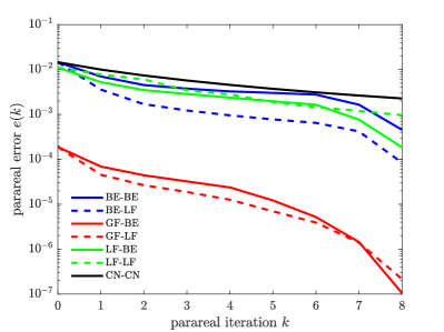
(a) $\boldsymbol{\mu}^{\star}_{1}=(1.6603,0.0229)$

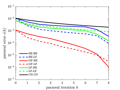
(b) $\boldsymbol{\mu}^{\star}_{2}=(1.5025,0.0201)$

Fig. 5: Comparison of initialization and coarse-propagation methods. Convergence of six methods.

The figure highlights two important trends. First, the results empirically support the theoretical result discussed in Remark 4.6: namely, the global-forecast initialization exhibits superior stability properties to the local-forecast initialization. In both online parameter instances, global-forecast initialization produces a very small initial error, while local-forecast initialization produces a larger initial error despite its use of the same time-evolution data; backward-Euler and Crank–Nicolson initialization produces a slightly smaller initial error than the local forecast. Second, note that the local-forecast propagator outperforms the backward-Euler coarse propagator when either the backward-Euler or global-forecasting initializations are employed.

To gain additional insight into the convergence properties of the methods, Figure 6 reports the convergence of the 51st entry of the state vector over parareal iterations for online parameter instance $\boldsymbol{\mu}^{\star}_{2}$, and Figure 7 reports convergence of the error in this quantity. These results highlight the two trends mentioned above; specifically, global-forecast initialization leads to a nearly exact initial solution, local-forecast initialization leads to a very poor initial solution, and local-forecast coarse propagation reduces errors more quickly than backward-Euler coarse propagation, even when backward-Euler initialization is employed; these plots do not include the CN-CN results, as they are very similar to the BE-BE results.

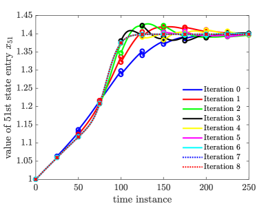
(a) BE-BE

(b) BE-LF

(c) LF-BE

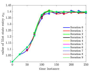
(d) LF-LF

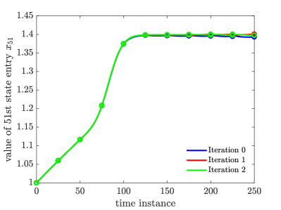
(e) GF-BE

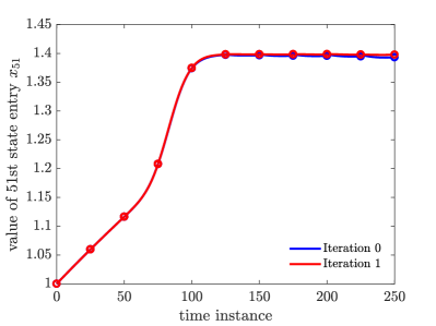
(f) GF-LF

Fig. 6: Comparison of initialization and coarse-propagation methods. Convergence of the 51st entry of the state vector for $\boldsymbol{\mu}^{\star}_{2}=(1.5025,0.0201)$ for six methods.

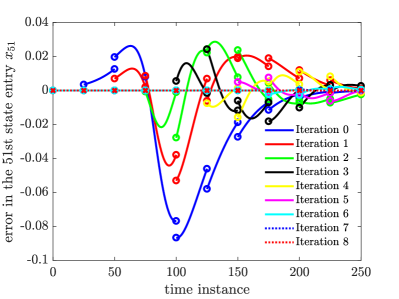
(a) BE-BE

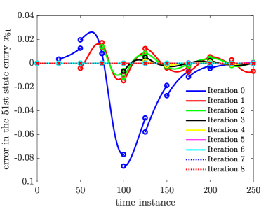
(b) BE-LF

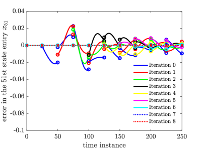
(c) LF-BE

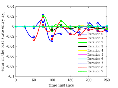
(d) LF-LF

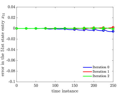
(e) GF-BE

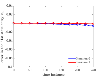
(f) GF-LF

Fig. 7: Comparison of initialization and coarse-propagation methods. Converence of the error in the 51st entry of the state vector (with respect to the serial solution) for $\boldsymbol{\mu}^{\star}_{2}=(1.5025,0.0201)$ for six methods.

In the remainder of the numerical experiments, we limit our focus to the typical parareal methods BE-BE and CN-CN, as well as the most promising proposed data-driven method GF-LF.

6.3 Ideal case

This section assesses performance of the method under the ‘ideal case’, i.e., when Assumptions A3–A5 are satisfied as discussed in Sections 4.1.2 and 4.2.2. Here, we ensure these conditions are met by repeating the training for each online point (i.e., $N_{\text{train}}=1$ with both the training point set equal to the online point) and employing ${\bar{N}}={\hat{N}}$. Recall that under these conditions, the coarse propagator is exact (Theorem 3), and the GF-LF method should converge after parareal initialization (hence require $K=0$ parareal iterations) and produce speedups given by Eq. (24) (Theorem (7)). Note that these conditions are ‘ideal’ for the proposed methodology, but not for typical parareal methods BE-BE or CN-CN. We assess memories of $\alpha=1,2,4,6$ and employ a termination tolerance of $\epsilon={5\times 10^{-4}}$ in this section only.

In the remaining experiments, we report the theoretical speedups derived in Section 4.2 due to the lack of reliability in timings obtained with our Matlab implementation. Here, the speedup for method GF-LF is provided by Eq. (23), and the speedup for methods BE-BE and CN-CN are provided by the following theorem, whose proof can be found in Appendix A.

Theorem 14 (Speedup: fine propagator as coarse propagator).

If the same time integrator is used for both the coarse and fine propagator and Assumption A8 holds, then the parareal method realizes a speedup of

(47) $$S_{\textit{fine}}({K})\vcentcolon=\frac{m}{({M}+{\bar{m}}-\frac{1}{2}{K})({K}+1)}.$$

Figures 8(a)–8(b) report the number of parareal iterations required for convergence when the number of coarse time instances ${M}$ increases (and the coarse time step $H=T_{\mathrm{final}}/{M}$ undergoes an attendant decrease). As expected, in all cases, the proposed GF-LF method converges in the minimum number of parareal iterations (i.e., ${K}=0$). In contrast, the BE-BE and CN-CN methods converge in the worst-case number of iterations (i.e., ${K}={M}-1$) for ${M}\leq 6$ in both cases; this occurs because these cases correspond to relatively large coarse time steps $H$, which degrades the accuracy of the backward-Euler and Crank–Nicolson schemes. The number of parareal iterations needed for convergence in the BE-BE and CN-CN cases decreases as the number of coarse time instances ${M}$ increases; this can be attributed to the decreasing coarse time step $H$, which improves the accuracy of the time integrators.

Figures 8(c)–8(d) report the theoretical speedups of these methods under these ideal conditions. Here, the reported values correspond to Eq. (47) for the BE-BE and CN-CN methods and Eq. (23) for the GF-LF method. As expected, the proposed technique yields near-ideal theoretical speedups, while the typical approaches produce modest speedups due to their slow convergence on this problem. Note that increasing the memory degrades speedup in this case, as all values for the memory ensure an exact initial solution in the ideal case; thus, employing a small memory does not degrade convergence here.

Finally, Figures 8(e)–8(f) report parareal convergence for these methods for ${M}=10$. As expected, the proposed GF-LF method produces a (near) zero error after initialization; on the other hand, the typical BE-BE and CN-CN methods exhibit relatively slow convergence.

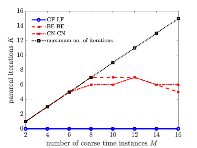
(a) $\boldsymbol{\mu}^{\star}_{1}=(1.6603,0.0229)$

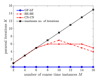
(b) $\boldsymbol{\mu}^{\star}_{2}=(1.5025,0.0201)$

(c) $\boldsymbol{\mu}^{\star}_{1}=(1.6603,0.0229)$

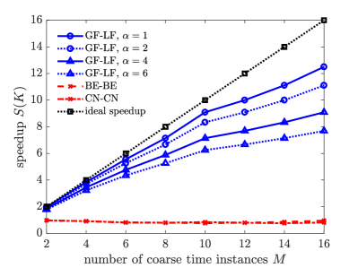
(d) $\boldsymbol{\mu}^{\star}_{2}=(1.5025,0.0201)$

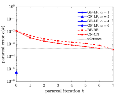
(e) $\boldsymbol{\mu}^{\star}_{1}=(1.6603,0.0229)$

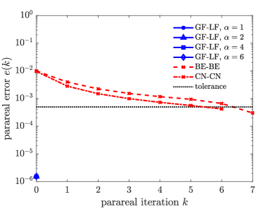
(f) $\boldsymbol{\mu}^{\star}_{2}=(1.5025,0.0201)$

Fig. 8: Ideal case. Number of parareal iterations ${K}$ required for convergence, theoretical speedups computed via Eq. (47) for BE-BE and Eq. (23) for GF-LF, and convergence plots. Figures (e) and (f) associate with ${M}=10$.

6.4 Predictive case

We now return to the original problem setup with $N_{\text{train}}=4$ training points and $N_{\text{online}}=2$ online points. Here, the ‘ideal case’ Assumptions A3–A5 no longer hold. To assess the accuracy of the coarse propagator in this predictive scenario, Figure 9 reports the relative projection error

(48) $$\varepsilon_{j}(\boldsymbol{\mu})\vcentcolon=\|(\mathbf{I}_{m}-\mathbf{\Xi}_{j}[\mathbf{\Xi}_{j}]^{T}){\mathbf{h}}(\hat{x}_{j}(\cdot,\boldsymbol{\mu}))\|/\|{\mathbf{h}}(\hat{x}_{j}(\cdot,\boldsymbol{\mu}))\|$$

$j\in{\rm Nature}{{\hat{N}}}$, which measures the ability of the temporal bases $\mathbf{\Xi}_{j}$ to capture the time evolution of the reduced states. Note that this is a global variant of the quantity that appears in the coarse-propagator error bound in Theorem 1 and measures the extent to which Assumption A3 is violated. Further, note that $\varepsilon_{j}=0$, $j\in{\rm Nature}{{\hat{N}}}$ for the ideal case. This figure also reports the relative magnitude of each reduced state

(49) $$m_{j}(\boldsymbol{\mu})\vcentcolon=\|{\mathbf{h}}(\hat{x}_{j}(\cdot,\boldsymbol{\mu}))\|/\|{\mathbf{h}}(\hat{\mathbf{x}}(\cdot,\boldsymbol{\mu}))\|,j\in{\rm Nature}{{\hat{N}}}.$$

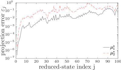
(a) Projection error $\varepsilon_{j}$, $j\in{\rm Nature}{{\hat{N}}}$

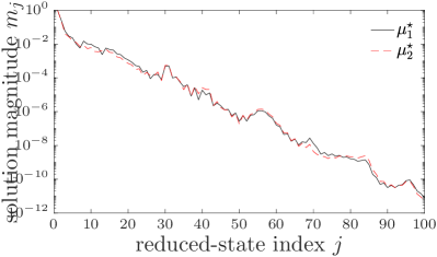
(b) Solution magnitude $m_{j}$, $j\in{\rm Nature}{{\hat{N}}}$

Fig. 9: Predictive case. Projection error and solution magnitude for online points $\boldsymbol{\mu}^{\star}_{1}$ and $\boldsymbol{\mu}^{\star}_{2}$.

Figure 9 shows that the temporal bases are more accurate (i.e., yield smaller projection errors) for online point $\boldsymbol{\mu}^{\star}_{1}$ than for $\boldsymbol{\mu}^{\star}_{2}$; this suggests that the method should perform better (i.e., converge in fewer parareal iterations) for the first online point. Thus, we can interpret $\boldsymbol{\mu}^{\star}_{1}$ and $\boldsymbol{\mu}^{\star}_{2}$ as providing increasingly difficult scenarios for the proposed method in which the time-evolution bases are increasingly inaccurate. In addition, the figure shows an inverse relationship between the projection error and the solution magnitude. This is intuitive: the time-evolution bases are able to accurately capture the time-evolution of the dominant (low-index) reduced states, while the ‘noisy’ (high-index) reduced states yield large projection errors. Section 6.5 explores this effect further.

Figures 10(a)–10(b) report the dependence of the number of parareal iterations on the number of coarse time instances ${M}$ for this case. Similar to the ideal case, the proposed GF-LF method converges in considerably fewer iterations than the BE-BE and CN-CN methods; in fact it converges in the minimum number of iterations ${K}=0$ for $\boldsymbol{\mu}^{\star}_{1}$. Also, the proposed GF-LF method exhibits better performance for $\boldsymbol{\mu}^{\star}_{1}$ than $\boldsymbol{\mu}^{\star}_{2}$ as was suggested by the projection errors in Figure 9. As before, the BE-BE and CN-CN methods converge in the worst-case number of iterations (i.e., ${K}={M}-1$) for ${M}\leq 8$ for both online points. However, for ${M}\geq 9$, the CN-CN method converges in fewer iterations than the BE-BE method, likely due to its higher-order accuracy. Figures 10(c)–10(d) report the theoretical speedups of both methods under these ideal conditions. Again, the proposed technique yields better speedups compared with the typical methods, which is apparent for $\boldsymbol{\mu}^{\star}_{1}$ in particular.

Finally, Figures 10(e)–10(f) report parareal convergence for both methods for ${M}=10$. The proposed GF-LF method produces a small error after initialization; for $\boldsymbol{\mu}^{\star}_{i}$, the error is smaller than the specified threshold for convergence. In contrast, the BE-BE and CN-CN methods exhibit relatively slow convergence with CN-CN converging faster, likely due to its higher-order accuracy.

These promising results suggest that the proposed GF-LF method can deliver significant performance improvements over standard parareal techniques, even when ideal conditions do not hold. We note that numerical results obtained for ${\hat{N}}=50$ (i.e., a less accurate reduced-order model) reproduce exactly the results reported in Figure 10, which correspond to ${\hat{N}}=100$. This reflects the fact that the proposed method’s performance is not directly tied to the accuracy of the reduced-order model; rather, it depends on the ability of the time-evolution bases to capture the time evolution of the reduced states as discussed above.

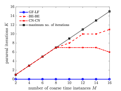
(a) $\boldsymbol{\mu}^{\star}_{1}=(1.6603,0.0229)$

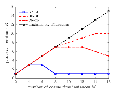
(b) $\boldsymbol{\mu}^{\star}_{2}=(1.5025,0.0201)$

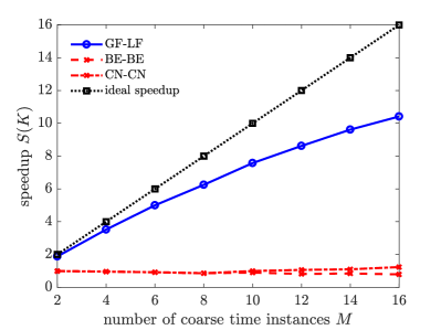
(c) $\boldsymbol{\mu}^{\star}_{1}=(1.6603,0.0229)$

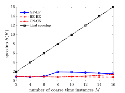
(d) $\boldsymbol{\mu}^{\star}_{2}=(1.5025,0.0201)$

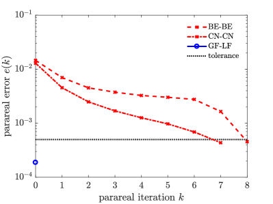
(e) $\boldsymbol{\mu}^{\star}_{1}=(1.6603,0.0229)$

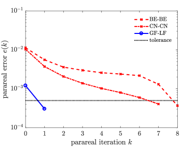
(f) $\boldsymbol{\mu}^{\star}_{2}=(1.5025,0.0201)$

Fig. 10: Predictive case. Number of parareal iterations ${K}$ required for convergence, theoretical speedups computed via Eq. (47) for BE-BE and Eq. (23) for GF-LF, and convergence plots. Figures (e) and (f) associate with ${M}=10$.

6.5 Parameter study

We now assess the dependence of the proposed GF-LF method on its parameters, namely the number of restricted variables ${\bar{N}}$ and the memory $\alpha$.

We first assess the effect of the number of restricted variables ${\bar{N}}$. Recall from Figure 9 that there is an inverse relationship between projection error and solution magnitude. In particular, low-index reduced states have large solution magnitudes and yield low projection errors; high-index reduced states comprise ‘noise’ that cannot be accurately forecasted due to their high projection errors. To gain additional insight into this, Figure 11 plots the global temporal bases $\mathbf{\Xi}_{j}$ associated with different (restricted) solution components.

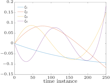
(a) $\mathbf{\Xi}_{1}$

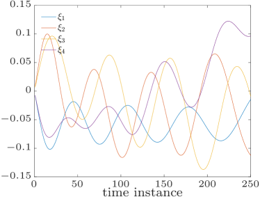
(b) $\mathbf{\Xi}_{10}$

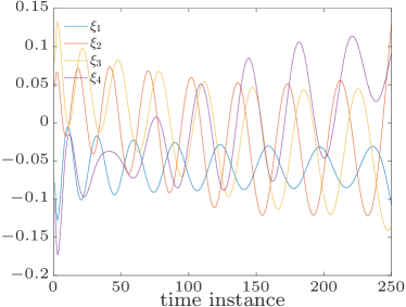
(c) $\mathbf{\Xi}_{20}$

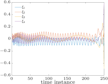
(d) $\mathbf{\Xi}_{100}$

Fig. 11: Parameter study. Visualization of global time-evolution bases $\mathbf{\Xi}_{j}$, $j\in\{1,10,20,100\}$. Time-evolution bases for high-index POD modes are more highly oscillatory; thus, high-index modes are less amenable to forecasting.

Note that the basis vectors are highly oscillatory for high-index modes, which is consistent with their low relative magnitudes and interpretation as solution ‘noise,’ as well as their associated large projection errors. This is consistent with the discussion in Remark 4.2: selecting a small value of ${\bar{N}}$ amounts to forecasting a small number of solution components, which increases the quantity $\|{\mathbf{R}^{T}_{\perp}}\mathcal{F}({\boldsymbol{\xi}};{T}^{{{n}}},{T}^{{{n}}+1})\|$ appearing in the bound (1) for the coarse-propagator error; alternatively, employing a large value of ${\bar{N}}$ increases the second term in bound (1) due to the large projection errors for high-index reduced states. Thus, we expect an intermediate value of ${\bar{N}}$ to yield the fastest convergence. Figure 12 reports convergence of the method for $\alpha=8$ for a range of values for ${\bar{N}}$. These results show precisely what we expect: the best performance is obtained (roughly) for an intermediate value of ${\bar{N}}=8$.

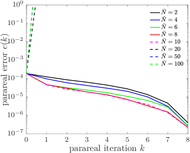
(a) $\boldsymbol{\mu}^{\star}_{1}=(1.6603,0.0229)$

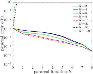
(b) $\boldsymbol{\mu}^{\star}_{2}=(1.5025,0.0201)$

Fig. 12: Parameter study. Convergence plots for the GF-LF method for a range of values for ${\bar{N}}$ and a memory of $\alpha=8$. Note that a value of ${\bar{N}}=8$ yields roughly the best overall performance.

We next consider the effect of the restricted-state dimension ${\bar{N}}$ purely when performing global-forecast initialization. We find that the the parareal error after initialization is ${e}(0)=1.88\times 10^{-4}$ for $\boldsymbol{\mu}^{\star}_{1}$ and ${e}(0)=1.21\times 10^{-3}$ for $\boldsymbol{\mu}^{\star}_{{2}}$ and for ${\bar{N}}\in\{6,8,10,15,20,25,30\}$ and a (fixed) memory of $\alpha=8$. Thus, initialization error is insensitive to the parameter ${\bar{N}}$; this is an artifact of the intrinsic stability of the global forecast as discussed in Remark 4.6. Further, it suggests that the first few restricted POD modes dominate the state information content.

Next, Figure 13 reports performance of the method for a fixed value of ${\bar{N}}=8$ and a range of values for the memory $\alpha$. First, note that interpolation, which corresponds to $\alpha={a}=4$, yields the worst performance in terms of error at a given iteration. This supports the theoretical results discussed in Remark 4.1: oversampling (i.e., employing $\alpha>{a}$) produces a stabilizing effect. In this case, the value of the memory leading to best overall performance (in terms of accuracy) is $\alpha=8$. Note that employing the smallest value for the memory yields the best theoretical speedups if the method were to converge in the same number of parareal iterations for all values of the memory. This illustrates the tradeoff discussed in Remark 4.3: increasing the memory $\alpha$ reduces the speedup for a fixed number of iterations needed for convergence; yet, doing so can also decrease the bound for the error between coarse and fine propagators, which promotes convergence.

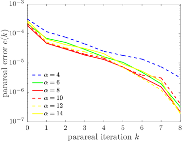
(a) $\boldsymbol{\mu}^{\star}_{1}=(1.6603,0.0229)$

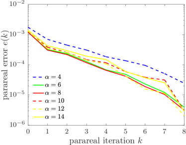
(b) $\boldsymbol{\mu}^{\star}_{2}=(1.5025,0.0201)$

(c) $\boldsymbol{\mu}^{\star}_{1}=(1.6603,0.0229)$

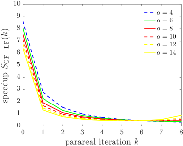
(d) $\boldsymbol{\mu}^{\star}_{2}=(1.5025,0.0201)$

Fig. 13: Parameter study. Convergence plots for the GF-LF method for a range of values for $\alpha$ and a value of ${\bar{N}}=8$. Note that a value of $\alpha=8$ yields the best overall performance.

7 Conclusions

This work presented a novel data-driven method for time parallelism. We applied both local and global forecasting to define initialization methods, as well as local forecasting to define the coarse propagator. These methods are data-driven, as they leverage the availability of time-domain data from which low-dimensional time-evolution bases for the state can be extracted; further, they are well-suited for POD-based reduced-order models, as the required time-domain data are already available. We performed analysis demonstrating the method’s accuracy, speedup, and stability. Key theoretical results include:

• The error between the local-forecast coarse propagator and the fine propagator can be bounded by a readily interpretable quantity (Theorem 1),

• Ideal conditions exist under which the local-forecast coarse propagator is equal to the fine propagator (Theorem 3), and

• The parareal recurrence is stable with the local-forecast coarse propagator (Theorem 11) with constants that are independent of the time discretization (Remark 4.5 and Figure 4).

• Existing convergence results for the parareal recurrence hold with the proposed coarse propagator, and superlinear convergence can be obtained under certain conditions (Corollary 13).

Key results corroborated by both theoretical analysis and numerical experiments include:

• Global-forecast initialization is more stable (Remark 4.6) and produces a more accurate solution (Figure 5) than the local-forecast initialization,

• Local-forecast coarse propagation is nearly always more accurate than backward-Euler coarse propagation, regardless of initialization (Figure 5),

• Under ideal conditions, the proposed method converges after parareal initialization, i.e., for ${K}=0$ in Algorithm 1 (Theorems 6–7 and Figures 8(a)–8(b)), and can realize near-ideal speedups (Figures 3 and 8(c)–8(d)),

• Increasing the memory $\alpha$ can improve coarse-propagation accuracy, but incurs a larger cost (Remark 4.1 and Figure 13), and

• Increasing the number of variables included in the forecast ${\bar{N}}$ has two competing effects: it can improve the forecast accuracy, but can incur error if the additional variables are difficult to forecast, e.g., associate with high-frequency temporal content (Remark 4.2 and Figures 9 and 12).

Finally, numerical experiments show that in all (predictive) cases where ideal conditions do not hold, global-forecast initialization and local-forecast coarse propagation outperforms backward-Euler initialization and coarse propagation (Figures 5 and 10).

Future work involves applying the proposed methodology in parallel computing environments with realistic timings, applying the method to parameterized full-order ODEs (i.e., not reduced-order models), and assessing the viability of alternative data sources (including physical experiments) to produce low-dimensional time-evolution bases.

Appendix A Proofs

• Proof of Theorem 1.  Under Assumptions A1 and A2, we have

  (50) $$\begin{split}\|\mathcal{F}({\boldsymbol{\xi}};{T}^{{{n}}},{T}^{{{n}}+1})-&{\mathcal{G}_{\mathrm{LF}}}({\boldsymbol{\xi}};{T}^{{{n}}},{T}^{{{n}}+1})\|=\|{\mathbf{P}_{\perp}}{\mathbf{R}^{T}_{\perp}}\mathcal{F}({\boldsymbol{\xi}};{T}^{{{n}}},{T}^{{{n}}+1})+{\mathbf{P}}{\mathbf{R}^{T}}\mathcal{F}({\boldsymbol{\xi}};{T}^{{{n}}},{T}^{{{n}}+1})-{\mathcal{G}_{\mathrm{LF}}}({\boldsymbol{\xi}};{T}^{{{n}}},{T}^{{{n}}+1})\|\\ &\leq M_{\mathbf{P}_{\perp}}\|{\mathbf{R}^{T}_{\perp}}\mathcal{F}({\boldsymbol{\xi}};{T}^{{{n}}},{T}^{{{n}}+1})\|+\underbrace{\|{\mathbf{P}}{\mathbf{R}^{T}}\mathcal{F}({\boldsymbol{\xi}};{T}^{{{n}}},{T}^{{{n}}+1})-{\mathcal{G}_{\mathrm{LF}}}({\boldsymbol{\xi}};{T}^{{{n}}},{T}^{{{n}}+1})\|}_{\text{(I)}}.\end{split}$$

  We can bound Term (I) using Eqs. (13) and (15) and A2 as follows:

  (51) (I) $$\leq M_{\mathbf{P}}\|{\mathbf{R}^{T}}\mathcal{F}({\boldsymbol{\xi}};{T}^{{{n}}},{T}^{{{n}}+1})-\left[{\mathcal{G}_{\mathrm{LF}}}_{1}^{{{n}}}({\boldsymbol{\xi}})\ \cdots\ {\mathcal{G}_{\mathrm{LF}}}_{{\bar{N}}}^{{{n}}}({\boldsymbol{\xi}})\right]^{T}\|=M_{\mathbf{P}}\|\boldsymbol{\delta}^{{{n}}}({\boldsymbol{\xi}})\|,$$

  where we have defined $\boldsymbol{\delta}^{{{n}}}({\boldsymbol{\xi}})\vcentcolon=[\delta_{1}^{{{n}}}({\boldsymbol{\xi}})\ \cdots\ \delta_{{\bar{N}}}^{{{n}}}({\boldsymbol{\xi}})]^{T}$ as the vector of errors in the local forecast, with

  (52) $$\delta_{j}^{{{n}}}({\boldsymbol{\xi}}) \vcentcolon={\mathbf{r}^{T}_{j}}\mathcal{F}({\boldsymbol{\xi}};{T}^{{{n}}},{T}^{{{n}}+1})-{\mathcal{G}_{\mathrm{LF}}}_{j}^{{{n}}}({\boldsymbol{\xi}})$$

  (56) $$=\mathbf{e}_{{\bar{m}}}^{T}\left(\mathbf{I}_{{\bar{m}}}-\mathbf{\Xi}_{j}^{{n}}\left[{{\mathbf{Z}}_{0}}\mathbf{\Xi}_{j}^{{n}}\right]^{+}{{\mathbf{Z}}_{0}}\right)\left[\begin{array}[]{c}{\mathbf{r}^{T}_{j}}\mathcal{F}({\boldsymbol{\xi}};{T}^{{{n}}},t^{{{{\bar{m}}}}{{n}}+1})-{\mathbf{r}^{T}_{j}}{\boldsymbol{\xi}}\\ \vdots\\ {\mathbf{r}^{T}_{j}}\mathcal{F}({\boldsymbol{\xi}};{T}^{{{n}}},{T}^{{{n}}+1})-{\mathbf{r}^{T}_{j}}{\boldsymbol{\xi}}\end{array}\right].$$

  Using the norm-equivalence relation $\|{\bf x}\|_{2}\leq\|{\bf x}\|_{1}$, we have from (51) that $\text{(I)}\leq M_{\mathbf{P}}\sum_{j=1}^{\bar{N}}|\delta_{j}^{{{n}}}({\boldsymbol{\xi}})|$ with

  (60) $$|\delta_{j}^{{{n}}}({\boldsymbol{\xi}})| \leq\Big{\|}\left(\mathbf{I}_{{\bar{m}}}-\mathbf{\Xi}_{j}^{{n}}\left[{{\mathbf{Z}}_{0}}\mathbf{\Xi}_{j}^{{n}}\right]^{+}{{\mathbf{Z}}_{0}}\right)\left[\begin{array}[]{c}{\mathbf{r}^{T}_{j}}\mathcal{F}({\boldsymbol{\xi}};{T}^{{{n}}},t^{{{{\bar{m}}}}{{n}}+1})-{\mathbf{r}^{T}_{j}}{\boldsymbol{\xi}}\\ \vdots\\ {\mathbf{r}^{T}_{j}}\mathcal{F}({\boldsymbol{\xi}};{T}^{{{n}}},{T}^{{{n}}+1})-{\mathbf{r}^{T}_{j}}{\boldsymbol{\xi}}\end{array}\right]\Big{\|}$$

  (64) $$\leq\beta_{j}^{{{n}}}\Big{\|}(\mathbf{I}_{{\bar{m}}}-\mathbf{\Xi}_{j}^{{n}}[\mathbf{\Xi}_{j}^{{n}}]^{T})\left[\begin{array}[]{c}{\mathbf{r}^{T}_{j}}\mathcal{F}({\boldsymbol{\xi}};{T}^{{{n}}},t^{{{{\bar{m}}}}{{n}}+1})-{\mathbf{r}^{T}_{j}}{\boldsymbol{\xi}}\\ \vdots\\ {\mathbf{r}^{T}_{j}}\mathcal{F}({\boldsymbol{\xi}};{T}^{{{n}}},{T}^{{{n}}+1})-{\mathbf{r}^{T}_{j}}{\boldsymbol{\xi}}\end{array}\right]\Big{\|}.$$

  Here, we have used a bound for the gappy POD error [11, Appendix D] and orthogonality of the time-evolution bases $\mathbf{\Xi}_{j}^{{n}}$. Note that (60) expresses the bound in terms of the gappy POD approximation error of the time evolution (restricted) state, while (64) does so in terms of the orthogonal projection error onto the time-evolution bases. $\blacksquare$

• Proof of Lemma 2.  If Assumption A3 holds, then ${\mathbf{h}}({\mathbf{r}^{T}_{j}}{\mathbf{x}})=\mathbf{\Xi}_{j}\hat{\mathbf{r}}_{j}$ for some $\hat{\mathbf{r}}_{j}\in\mathbb{R}^{{a}}$. Applying the ${{n}}$th sampling matrix and utilizing quantities defined in Algorithm 3 with Assumption A4 (i.e., $\upsilon=1.0$) yields

  (65) $${\mathbf{Z}}^{{{n}}}{\mathbf{h}}({\mathbf{r}^{T}_{j}}{\mathbf{x}})={\mathbf{Z}}^{{{n}}}\mathbf{\Xi}_{j}\hat{\mathbf{r}}_{j}=\begin{bmatrix}\mathbf{u}^{k}_{1}\ \cdots\ \mathbf{u}^{k}_{{a}}\end{bmatrix}\mathop{\operator@font diag}\nolimits(\sigma_{1},\ldots,\sigma_{{a}})\begin{bmatrix}\mathbf{v}^{k}_{1}\ \cdots\ \mathbf{v}^{k}_{{a}}\end{bmatrix}^{T}\hat{\mathbf{r}}_{j}=\mathbf{\Xi}_{j}^{{n}}\hat{\hat{\mathbf{r}}}_{j}^{{{n}}},$$

  where we have defined $\hat{\hat{\mathbf{r}}}_{j}^{{{n}}}\vcentcolon=\mathop{\operator@font diag}\nolimits(\sigma_{1},\ldots,\sigma_{{a}})\begin{bmatrix}\mathbf{v}^{k}_{1}\ \cdots\ \mathbf{v}^{k}_{{a}}\end{bmatrix}^{T}\hat{\mathbf{r}}_{j}$. Noting that ${\mathbf{r}^{T}_{j}}{\mathbf{x}}\in\mathcal{H}$ implies ${\mathbf{Z}}^{{{n}}}{\mathbf{h}}({\mathbf{r}^{T}_{j}}{\mathbf{x}})={\mathbf{h}^{{n}}}({\mathbf{r}^{T}_{j}}{\mathbf{x}})$, we have the desired result: ${\mathbf{h}^{{n}}}({\mathbf{r}^{T}_{j}}{\mathbf{x}})\in\mathrm{Ran}(\mathbf{\Xi}_{j}^{{n}})$, $j\in{\rm Nature}{N}$, ${{n}}\in\mathbb{N}_{0}({M}-1)$. $\blacksquare$

• Proof of Theorem 3.  Under Assumptions A3 and A4, we have from Lemma 2 that ${\mathbf{h}^{{n}}}({\mathbf{r}^{T}_{j}}{\mathbf{x}})\in\mathrm{Ran}(\mathbf{\Xi}_{j}^{{n}})$, $j\in{\rm Nature}{N}$, ${{n}}\in\mathbb{N}_{0}({M}-1)$. Then, from Eqs. (9), (11), and (13) it follows

  $${f}_{j}^{{n}}({\mathbf{r}^{T}_{j}}\mathcal{f}^{{{n}}}({\mathbf{x}}({T}^{{{n}}}));{T}^{{{n}}},{T}^{{{n}}+1}) ={f}_{j}^{{n}}({\mathbf{r}^{T}_{j}}{\mathbf{x}};{T}^{{{n}}},{T}^{{{n}}+1})={\mathbf{r}^{T}_{j}}{\mathbf{x}}({T}^{{{n}}})+\mathbf{e}_{{{{\bar{m}}}}{{n}}+1-{{{\bar{m}}}}{{n}}}^{T}\mathbf{\Xi}_{j}^{{n}}[{{\mathbf{Z}}_{0}}\mathbf{\Xi}_{j}^{{n}}]^{+}{{\mathbf{Z}}_{0}}{\mathbf{h}^{{n}}}({\mathbf{r}^{T}_{j}}{\mathbf{x}})$$

  $$={\mathbf{r}^{T}_{j}}{\mathbf{x}}({T}^{{{n}}})+\mathbf{e}_{{{{\bar{m}}}}{{n}}+1-{{{\bar{m}}}}{{n}}}^{T}\mathbf{\Xi}_{j}^{{n}}\hat{\hat{\mathbf{r}}}_{j}^{{{n}}}$$

  $$={\mathbf{r}^{T}_{j}}{\mathbf{x}}({T}^{{{n}}})+\mathbf{e}_{{{{\bar{m}}}}{{n}}+1-{{{\bar{m}}}}{{n}}}^{T}{\mathbf{h}^{{n}}}({\mathbf{r}^{T}_{j}}{\mathbf{x}})={\mathbf{r}^{T}_{j}}{\mathbf{x}}({T}^{{{n}}+1})={\mathbf{r}^{T}_{j}}\mathcal{F}({\mathbf{x}}({T}^{{{n}}});{T}^{{{n}}},{T}^{{{n}}+1}),$$

  where we have used ${\mathbf{h}^{{n}}}({\mathbf{r}^{T}_{j}}{\mathbf{x}})=\mathbf{\Xi}_{j}^{{n}}\hat{\hat{\mathbf{r}}}_{j}^{{{n}}}$ from Eq. (65) and $[{{\mathbf{Z}}_{0}}\mathbf{\Xi}_{j}^{{n}}]^{+}{{\mathbf{Z}}_{0}}\mathbf{\Xi}_{j}^{{n}}=\mathbf{I}$. Leveraging Assumption A5 (i.e., ${\mathbf{P}}{\mathbf{R}^{T}}=\mathbf{I}_{N}$ with $N={\bar{N}}$) along with the definition of the coarse propagator (15) yields the desired result. $\blacksquare$

• Proof of Theorem 4.  Under Assumption A8, the wall time incurred by a serial solution is $m\tau_{\mathcal{F}}$, where $\tau_{\mathcal{F}}\in\mathbb{R}_{+}$ is the wall time required to compute $\mathcal{F}({\mathbf{x}}(t^{{{n}}});t^{{{n}}},t^{{{n}}+1})$ for a given ${{n}}\in\mathbb{N}_{0}(m-1)$.

  Under Assumptions A6 and A8, the wall time incurred by initializing the proposed method in Steps 1–5 of Algorithm 1 is composed of (1) the local-forecast initialization in Step 2 of Algorithm 1, which incurs performing (in serial) fine propagation $\alpha$ times in each coarse time interval (wall time of ${M}\alpha\tau_{\mathcal{F}}$) and (2) the (worst-case) parallel fine propagation in Steps 3–5 (wall time of $({\bar{m}}-\alpha)\tau_{\mathcal{F}}$); here, we have exploited the fact that we can reuse the first $\alpha$ fine propagations on each time interval, as these were computed during local-forecast initialization.

  Because the local forecast is also employed as a coarse propagator, Step 9 of Algorithm 1 can be replaced by simply setting $\mathbf{g}^{{{n}}+1}_{0}={\mathbf{x}}^{{{n}}+1}_{0}$, which incurs no cost under Assumption A8. Then, each subsequent iteration requires (1) serial coarse propagation in Step 14 (wall time of $({M}-{k})\alpha\tau_{\mathcal{F}}$), and (2) parallel fine propagation in Step 18 (wall time of $({\bar{m}}-\alpha)\tau_{\mathcal{F}}$). The ratio of these costs yields the theoretical speedup. Finally, we note that additional speedups may be realizable by pipelining operations, i.e., initiating the fine propagation on a given coarse time interval as soon as its initial value is available. $\blacksquare$

• Proof of Theorem 5.  Under Assumption A8, the wall time incurred by a serial solution is (again) $m\tau_{\mathcal{F}}$. Under Assumptions A7 and A8, the wall time incurred by initializing the proposed method in Steps 1–5 of Algorithm 1 is composed of (1) global-forecast initialization in Step 2 of Algorithm 1, which incurs performing fine propagation $\alpha$ times in only the first time interval (wall time of $\alpha\tau_{\mathcal{F}}$) and (2) the (worst-case) parallel fine propagation in Steps 3–5 (wall time of ${\bar{m}}\tau_{\mathcal{F}}$); note that we can no longer reuse fine propagation from initialization beyond the first time interval.

  Because the local forecast is employed as a coarse propagator, Step 9 of Algorithm 1 incurs parallel coarse propagation, which requires performing (in parallel) fine propagation $\alpha$ times in time intervals $1$ to ${M}-1$ (wall time of $\alpha\tau_{\mathcal{F}}$). Then, each subsequent iteration requires (1) serial coarse propagation in Step 14 (wall time of $({M}-{k})\alpha\tau_{\mathcal{F}}$), and (2) parallel fine propagation in Step 18 (wall time of $({\bar{m}}-\alpha)\tau_{\mathcal{F}}$). The ratio of these costs yields the theoretical speedup. $\blacksquare$

• Proof of Theorem 6.  We proceed by induction. Assume that ${\mathbf{x}}^{{{n}}}_{0}={\mathbf{x}}({T}^{{{n}}})$, which holds for ${{n}}=0$ by construction. Then, we have from Theorem 3 under Assumptions A3–A5 that ${\mathcal{G}_{\mathrm{LF}}}({\mathbf{x}}^{{{n}}}_{0};{T}^{{{n}}},{T}^{{{n}}+1})={\mathbf{x}}({T}^{{{n}}+1})$. Under Assumption A6 (i.e., initialization is performed via local forecasting), we have ${\mathbf{x}}^{{{n}}+1}_{0}={\mathcal{G}_{\mathrm{LF}}}({{\mathbf{x}}^{{{n}}}_{0}};{{T}^{{{n}}}},{{T}^{{{n}}+1}})={\mathbf{x}}({T}^{{{n}}+1}).$ By induction, this yields ${\mathbf{x}}^{{{n}}}_{0}={\mathbf{x}}({T}^{{{n}}})$, ${{n}}\in\mathbb{N}_{0}({M})$. This means that the initialized values computed in Step 2 of Algorithm 1 are correct under the stated assumptions; as a result, the fine propagation performed in Steps 3–5 will complete computation of the correct solution, the error measure in Step 6 will evaluate to zero, and the algorithm will terminate with ${K}=0$. Finally, Theorem 4 is valid under Assumptions A6 and A8; thus, $S_{\mathrm{LF\text{-}LF}}(0)$ provides the theoretical speedup in this case. $\blacksquare$

• Proof of Theorem 7.  As in Lemma 2, if Assumption A3 holds, then ${\mathbf{h}}({\mathbf{r}^{T}_{j}}{\mathbf{x}})=\mathbf{\Xi}_{j}\hat{\mathbf{r}}_{j}$ for some $\hat{\mathbf{r}}_{j}\in\mathbb{R}^{{a}}$. Then, we have from Eqs. (6) and (8)

  (66) $$\begin{split}{f}_{j}({\mathbf{r}^{T}_{j}}\mathcal{f}({\mathbf{x}}^{0});0,{T}^{{{n}}})={f}_{j}({\mathbf{r}^{T}_{j}}{\mathbf{x}};0,{T}^{{{n}}})&={\mathbf{r}^{T}_{j}}{\mathbf{x}}(0)+\mathbf{e}_{{{{\bar{m}}}}{{n}}}^{T}\mathbf{\Xi}_{j}[{{\mathbf{Z}}_{0}}\mathbf{\Xi}_{j}]^{+}{{\mathbf{Z}}_{0}}\mathbf{\Xi}_{j}\hat{\mathbf{r}}_{j}={\mathbf{r}^{T}_{j}}{\mathbf{x}}(0)+\mathbf{e}_{{{{\bar{m}}}}{{n}}}^{T}\mathbf{\Xi}_{j}\hat{\mathbf{r}}_{j}\\ &={\mathbf{r}^{T}_{j}}{\mathbf{x}}(0)+\mathbf{e}_{{{{\bar{m}}}}{{n}}}^{T}{\mathbf{h}}({\mathbf{r}^{T}_{j}}{\mathbf{x}})={\mathbf{r}^{T}_{j}}{\mathbf{x}}({T}^{{{n}}}),\end{split}$$

  where we have used ${\mathbf{h}}({\mathbf{r}^{T}_{j}}{\mathbf{x}})=\mathbf{\Xi}_{j}\hat{\mathbf{r}}_{j}$ and $[{{\mathbf{Z}}_{0}}\mathbf{\Xi}_{j}]^{+}{{\mathbf{Z}}_{0}}\mathbf{\Xi}_{j}=\mathbf{I}$. Under Assumption A7 with the definition of the proposed global-forecast initialization (18), Assumption A5 (i.e., ${\mathbf{P}}{\mathbf{R}^{T}}=\mathbf{I}_{N}$), and the construction ${\mathbf{x}}^{0}_{0}={\mathbf{x}}^{0}={\mathbf{x}}({T}^{0})$, we then have ${\mathbf{x}}^{{{n}}}_{0}={\mathbf{x}}({T}^{{{n}}}),\ {{n}}\in\mathbb{N}_{0}({M}).$ As before, this proves the desired result under the stated assumptions: the initialized values computed in Step 2 of Algorithm 1 are correct. Thus, the fine propagation performed in Steps 3–5 will complete computation of the correct solution, the error measure in Step 6 will evaluate to zero, and the algorithm will terminate with ${K}=0$. Finally, Theorem 5 is valid under Assumptions A7 and A8; thus, $S_{\mathrm{GF\text{-}LF}}(0)$ provides the theoretical speedup in this case. $\blacksquare$

• Proof of Lemma 8.  Defining $A\vcentcolon=\alpha_{A}(1+C_{A}H)$ and $B\vcentcolon=\alpha_{B}(1+C_{B}H)$, we have from parareal recurrence (4) and bounds (25) and (26) that

  (67) $$\begin{split}\|{\mathbf{x}}^{{{{n}}}+1}_{{k}+1}\|\leq&A\|{\mathbf{x}}^{{{{n}}}}_{{k}+1}\|+B\|{\mathbf{x}}^{{{{n}}}}_{{k}}\|,\quad{{n}}\in\mathbb{N}_{0}({M}-1),\ {k}\in\mathbb{N}_{0}({{n}}),\end{split}$$

  which can be written equivalently as

  (68) $$\begin{split}\|{\mathbf{x}}^{{{{n}}}+1}_{{k}}\|\leq&A\|{\mathbf{x}}^{{{{n}}}}_{{k}}\|+B\|{\mathbf{x}}^{{{{n}}}}_{{k}-1}\|,\quad{{n}}\in\mathbb{N}_{0}({M}-1),\ {k}\in{\rm Nature}{{{n}}+1}.\end{split}$$

  We prove by induction over ${{n}}$ that

  (69) $$\|{\mathbf{x}}^{{{n}}}_{{k}}\|\leq A^{{n}}\|{\mathbf{x}}^{0}\|+\sum_{j=1}^{{n}}A^{{{n}}-j}B\|{\mathbf{x}}^{j-1}_{{k}-1}\|,\quad{{n}}\in{\rm Nature}{{M}},\ {k}\in{\rm Nature}{{{n}}}$$

  Applying inequality (67) with ${{n}}={k}=0$ yields $\|{\mathbf{x}}^{1}_{1}\|\leq A\|{\mathbf{x}}^{0}_{1}\|+B\|{\mathbf{x}}^{0}_{0}\|=(A+B)\|{\mathbf{x}}^{0}\|,$ where we have used $\|{\mathbf{x}}^{0}_{{k}}\|=\|{\mathbf{x}}^{0}\|$, ${k}\in\mathbb{N}_{0}({K})$ by construction. Thus, inequality (69) holds for ${{n}}=1$.

  Now assume that inequality (69) holds for some ${{n}}\in{\rm Nature}{{M}-1}$ and all ${k}\in{\rm Nature}{{{n}}}$; we will show that inequality (69) is then satisfied for ${{n}}+1\in\{2,\ldots,{M}\}$. Applying inequality (68) with ${{n}}\in{\rm Nature}{{M}-1}$, ${k}\in{\rm Nature}{{{n}}+1}$ yields

  (70) $$\|{\mathbf{x}}^{{{n}}+1}_{{k}}\| \leq A\|{\mathbf{x}}^{{{n}}}_{{k}}\|+B\|{\mathbf{x}}^{{{n}}}_{{k}-1}\|\leq A\Big{(}A^{{n}}\|{\mathbf{x}}^{0}\|+\sum_{j=1}^{{n}}A^{{{n}}-j}B\|{\mathbf{x}}^{j-1}_{{k}-1}\|\Big{)}+B\|{\mathbf{x}}^{{{n}}}_{{k}-1}\|$$

  (71) $$\leq A^{{{n}}+1}\|{\mathbf{x}}^{0}\|+\sum_{j=1}^{{{n}}+1}A^{{{n}}+1-j}B\|{\mathbf{x}}^{j-1}_{{k}-1}\|,\quad{{n}}\in{\rm Nature}{{M}-1},\ {k}\in{\rm Nature}{{{n}}+1},$$

  which is Eq. (69) for ${{n}}+1\in\{2,\ldots,{M}\}$.

  We now prove that

  (72) $$\|{\mathbf{x}}^{{{n}}}_{{k}}\|\leq(A+B)^{{n}}\|{\mathbf{x}}^{0}\|,\quad{{n}}\in{\rm Nature}{{M}},\ {k}={{n}}.$$

  Applying inequality (67) with ${k}={{n}}$ yields $\|{\mathbf{x}}^{{{n}}}_{{{n}}}\|\leq A\|{\mathbf{x}}^{{{n}}-1}_{{{n}}}\|+B\|{\mathbf{x}}^{{{n}}-1}_{{{n}}-1}\|,\quad{{n}}\in{\rm Nature}{{M}}.$ From the finite-termination property in Eq. (5), we have that ${\mathbf{x}}^{{{n}}-1}_{{{n}}}={\mathbf{x}}^{{{n}}-1}_{{{n}}-1}={\mathbf{x}}({T}^{{{n}}-1})$, thus this inequality becomes $\|{\mathbf{x}}^{{{n}}}_{{{n}}}\|\leq A\|{\mathbf{x}}^{{{n}}-1}_{{{n}}-1}\|+B\|{\mathbf{x}}^{{{n}}-1}_{{{n}}-1}\|\leq(A+B)\|{\mathbf{x}}^{{{n}}-1}_{{{n}}-1}\|$ from which the desired result directly follows.

Substituting the definitions of $A$ and $B$ in inequalities (69)–(72), employing the generalized binomial formula, and applying the inequality $(1+x)^{n}\leq\exp(nx)$ yields the desired result. $\blacksquare$

• Proof of Lemma 9.  From Eqs. (11) and (13), Assumptions A9 and A10, and the norm-equivalence relation $\|{\bf x}\|_{2}\leq\sqrt{n}\|{\bf x}\|_{\infty}$ for ${\bf x}\in\mathbb{R}^{n}$, Eq. (14) yields

  (73) $$|{\mathcal{G}_{\mathrm{LF}}}_{j}^{{{n}}}({\boldsymbol{\xi}})| \leq|(1-\sum_{i=1}^{\alpha}{\gamma}_{ij}^{{n}}){\mathbf{r}^{T}_{j}}{\boldsymbol{\xi}}|+|\sum_{i=1}^{\alpha}{\gamma}_{ij}^{{n}}{\mathbf{r}^{T}_{j}}\mathcal{F}({\boldsymbol{\xi}};{T}^{{{n}}},t^{{{{\bar{m}}}}{{n}}+i})|$$

  (74) $$=|(1-\sum_{i=1}^{\alpha}{\gamma}_{ij}^{{n}}){\mathbf{r}^{T}_{j}}{\boldsymbol{\xi}}|+|\mathbf{e}_{{\bar{m}}}^{T}\mathbf{\Xi}_{j}^{{n}}\left[{{\mathbf{Z}}_{0}}\mathbf{\Xi}_{j}^{{n}}\right]^{+}[{\mathbf{r}^{T}_{j}}\mathcal{F}({\boldsymbol{\xi}};{T}^{{{n}}},t^{{{{\bar{m}}}}{{n}}+1})\ \cdots\ {\mathbf{r}^{T}_{j}}\mathcal{F}({\boldsymbol{\xi}};{T}^{{{n}}},t^{{{{\bar{m}}}}{{n}}+\alpha})]^{T}|$$

  (75) $$\leq M_{{\mathbf{r}_{j}}}\left[|1-\sum_{i=1}^{\alpha}{\gamma}_{ij}^{{n}}|\|{\boldsymbol{\xi}}\|+\|\mathbf{e}_{{\bar{m}}}^{T}\mathbf{\Xi}_{j}^{{n}}\left[{{\mathbf{Z}}_{0}}\mathbf{\Xi}_{j}^{{n}}\right]^{+}\|\left(\sum_{{k}=1}^{\alpha}\|\mathcal{F}({\boldsymbol{\xi}};{T}^{{{n}}},t^{{{{\bar{m}}}}{{n}}+{k}})\|^{2}\right)^{1/2}\right]$$

  (76) $$\leq M_{{\mathbf{r}_{j}}}\left[\lambda_{j}^{{{n}}}+\kappa_{j}^{{{n}}}\sqrt{\alpha}(1+C_{\mathcal{F}}\alpha h)\right]\|{\boldsymbol{\xi}}\|=M_{{\mathbf{r}_{j}}}\left(\lambda_{j}^{{{n}}}+\kappa_{j}^{{{n}}}\sqrt{\alpha}\right)\left[1+\frac{\kappa_{j}^{{{n}}}\alpha^{3/2}C_{\mathcal{F}}h}{\lambda_{j}^{{{n}}}+\kappa_{j}^{{{n}}}\sqrt{\alpha}}\right]\|{\boldsymbol{\xi}}\|$$

  (77) $$=M_{{\mathbf{r}_{j}}}\left(\lambda_{j}^{{{n}}}+\kappa_{j}^{{{n}}}\sqrt{\alpha}\right)\left[1+\frac{(\alpha/{\bar{m}})\kappa_{j}^{{{n}}}\sqrt{\alpha}}{\lambda_{j}^{{{n}}}+\kappa_{j}^{{{n}}}\sqrt{\alpha}}C_{\mathcal{F}}H\right]\|{\boldsymbol{\xi}}\|.$$

  From Eq. (15) and Assumption A2 follows then $\|{\mathcal{G}_{\mathrm{LF}}}({\boldsymbol{\xi}};{T}^{{{{n}}}},{T}^{{{{n}}}+1})\|\leq\sqrt{{\bar{N}}}M_{\mathbf{P}}\max_{j\in{\rm Nature}{{\bar{N}}}}|{\mathcal{G}_{\mathrm{LF}}}_{j}^{{{n}}}({\boldsymbol{\xi}})|,$ which produces the desired result. $\blacksquare$

• Proof of Lemma 10.  Under the stated assumptions, we have

  (78) $$\begin{split}\|\mathcal{F}({\boldsymbol{\xi}};{T}^{{{n}}},{T}^{{{n}}+1})-{\mathcal{G}_{\mathrm{LF}}}({\boldsymbol{\xi}};{T}^{{{n}}},{T}^{{{n}}+1})\|=&\|{\mathbf{P}_{\perp}}{\mathbf{R}^{T}_{\perp}}\mathcal{F}({\boldsymbol{\xi}};{T}^{{{n}}},{T}^{{{n}}+1})+{\mathbf{P}}{\mathbf{R}^{T}}\mathcal{F}({\boldsymbol{\xi}};{T}^{{{n}}},{T}^{{{n}}+1})-{\mathcal{G}_{\mathrm{LF}}}({\boldsymbol{\xi}};{T}^{{{n}}},{T}^{{{n}}+1})\|\\ \leq&M_{\perp}(1+C_{\mathcal{F}}{H})\|{\boldsymbol{\xi}}\|+M_{\mathbf{P}}\|\boldsymbol{\delta}^{{{n}}}({\boldsymbol{\xi}})\|,\end{split}$$

  where we have used Eq. (51). Then from Eqs. (52) and (76), we have

  (79) $$|\delta_{j}^{{{n}}}({\boldsymbol{\xi}})|\leq |{\mathbf{r}^{T}_{j}}\mathcal{F}({\boldsymbol{\xi}};{T}^{{{n}}},{T}^{{{n}}+1})|+|{\mathcal{G}_{\mathrm{LF}}}_{j}^{{{n}}}({\boldsymbol{\xi}})|$$

  (80) $$\leq M_{{\mathbf{r}_{j}}}(1+C_{\mathcal{F}}H)\|{\boldsymbol{\xi}}\|+M_{{\mathbf{r}_{j}}}\left[\lambda_{j}^{{{n}}}+\kappa_{j}^{{{n}}}\sqrt{\alpha}(1+C_{\mathcal{F}}\alpha h)\right]\|{\boldsymbol{\xi}}\|$$

  (81) $$=M_{{\mathbf{r}_{j}}}(1+\lambda_{j}^{{{n}}}+\kappa_{j}^{{{n}}}\sqrt{\alpha}+(1+\kappa_{j}^{{{n}}}\sqrt{\alpha}(\alpha/{\bar{m}}))C_{\mathcal{F}}H)\|{\boldsymbol{\xi}}\|$$

  (82) $$=M_{{\mathbf{r}_{j}}}(1+\lambda_{j}^{{{n}}}+\kappa_{j}^{{{n}}}\sqrt{\alpha})(1+\frac{\kappa_{j}^{{{n}}}\sqrt{\alpha}(\alpha/{\bar{m}})+1}{\lambda_{j}^{{{n}}}+\kappa_{j}^{{{n}}}\sqrt{\alpha}+1}C_{\mathcal{F}}H)\|{\boldsymbol{\xi}}\|.$$

  Using the norm-equivalence relation $\|{\bf x}\|_{2}\leq\sqrt{n}\|{\bf x}\|_{\infty}$, we have $\|\boldsymbol{\delta}^{{{n}}}({\boldsymbol{\xi}})\|\leq\sqrt{{\bar{N}}}\max_{j\in{\rm Nature}{{\bar{N}}}}|\delta_{j}^{{{n}}}({\boldsymbol{\xi}})|.$ Combining inequalities (78), (82), and the above inequality yields

  $$\|\mathcal{F}({\boldsymbol{\xi}};{T}^{{{n}}},{T}^{{{n}}+1})-{\mathcal{G}_{\mathrm{LF}}}({\boldsymbol{\xi}};{T}^{{{n}}},{T}^{{{n}}+1})\|\leq M_{\perp}(1+C_{\mathcal{F}}{H})\|{\boldsymbol{\xi}}\|+\sqrt{{\bar{N}}}M_{\mathbf{P}}\max_{j\in{\rm Nature}{{\bar{N}}}}M_{{\mathbf{r}_{j}}}(\alpha_{j}^{n}+1)\left(1+D_{j}^{n}C_{\mathcal{F}}H\right)\|{\boldsymbol{\xi}}\|,$$

  where $D_{j}^{n}\vcentcolon=\frac{(\alpha/{\bar{m}})\kappa_{j}^{{{n}}}\sqrt{\alpha}+1}{\lambda_{j}^{{{n}}}+\kappa_{j}^{{{n}}}\sqrt{\alpha}+1}$. Noting that $D_{j}^{n}\leq 1$ because $\alpha/{\bar{m}}\leq 1$, this quantity can be bounded from above by the quantity that is the desired result. $\blacksquare$

• Proof of Theorem 11.  Under the stated assumptions, the results of Lemmas 9 and 10 hold. This implies that the conditions of Lemma 1 for $\mathcal{G}\leftarrow{\mathcal{G}_{\mathrm{LF}}}$ hold with the specified values of $\alpha_{A}$, $C_{A}$, $\alpha_{B}$, and $C_{B}$. $\blacksquare$

• Proof of Corollary 13.  Under Assumptions A11 and A14, the coarse propagator is the same on each coarse time interval, i.e., ${\mathcal{G}_{\mathrm{LF}}}^{i}={\mathcal{G}_{\mathrm{LF}}}^{j}={\mathcal{G}_{\mathrm{LF}}}$, and automatically satisfies Assumption A12, as the definition of the coarse propagator (16) simplifies to ${\mathcal{G}_{\mathrm{LF}}}:({\xi};{T}^{{{n}}},{T}^{{{n}}+1})\mapsto\bar{a}_{\text{LF}}{\xi}$. Thus, inequality (38) results from applying inequality (35) with $\bar{a}_{\mathcal{G}}\leftarrow\bar{a}_{\text{LF}}$. Next, Assumption A13 is automatically satisfied under Assumption A15 because $\bar{a}_{\text{LF}}=1+\sum_{i=1}^{\alpha}{\gamma}_{i}[(\bar{a}_{\mathcal{F}})^{i}-1]$. Therefore, inequality (39) results from applying inequality (37) with $\bar{a}_{\mathcal{G}}\leftarrow\bar{a}_{\text{LF}}$. $\blacksquare$

• Proof of Theorem 14.  Under Assumption A8, the wall time incurred by a serial solution is $m\tau_{\mathcal{F}}$, where $\tau_{\mathcal{F}}\in\mathbb{R}_{+}$ is the wall time required to compute $\mathcal{F}({\mathbf{x}}(t^{{{n}}});t^{{{n}}},t^{{{n}}+1})$ for a given ${{n}}\in\mathbb{N}_{0}(m-1)$. Further, the wall time incurred by initializing the proposed method in Steps 1–5 of Algorithm 1 is composed of (1) local-forecast initialization in Step 2 of Algorithm 1, which incurs ${M}$ applications of the time integrator (wall time of ${M}\tau_{\mathcal{F}}$) and (2) the (worst-case) parallel fine propagation in Steps 3–5 (wall time of $\tau_{\mathcal{F}}{\bar{m}}$).

  Because the coarse propagator was also employed for initialization, Step 9 of Algorithm 1 can be replaced by simply setting $\mathbf{g}^{{{n}}+1}_{0}={\mathbf{x}}^{{{n}}+1}_{0}$, which incurs no cost under Assumption A8. Then, each subsequent iteration requires (1) serial coarse propagation in Step 14 (wall time of $({M}-{k})\tau_{\mathcal{F}}$), and (2) parallel fine propagation in Steps 18 and 23 (wall time of $\tau_{\mathcal{F}}{\bar{m}}$). The ratio of these costs yields the theoretical speedup. As before, we note that additional speedups may be realizable by pipelining operations. $\blacksquare$

Appendix B Ideal conditions with Newton-solver initial guesses

We now consider the case of a nonlinear dynamical system wherein the forecasts are also employed to generate initial guesses for the Newton solver as proposed in Ref. [12]. We therefore introduce the following assumptions:

1. The velocity $\mathbf{g}$ is nonlinear.

2. The fine propagator corresponds to an implicit single-step scheme (i.e., $\mathcal{F}$ is such that $\mathbf{r}^{i}({\mathbf{x}}(t^{i})))=0$).

3. The Newton-solver initial guesses are provided by the local forecast, i.e., Newton’s method for solving $\mathbf{r}^{i}(\mathbf{w})=0$ with $t^{i}\in\mathcal{t}^{{{n}}}$ at parareal iteration ${k}$ employs

   $$\mathbf{w}^{i,(0)}={\mathbf{P}}[{f}_{1}^{{n}}({\mathbf{r}^{T}_{1}}\mathcal{f}^{{{n}}}({\mathbf{x}}^{{{n}}}_{{k}});{T}^{{{n}}},t^{i})\ \cdots\ {f}_{N}^{{n}}({\mathbf{r}^{T}_{N}}\mathcal{f}^{{{n}}}({\mathbf{x}}^{{{n}}}_{{k}});{T}^{{{n}}},t^{i})]^{T}$$

   as an initial guess.

4. The Newton-solver initial guesses are provided by the global forecast, i.e., Newton’s method for solving $\mathbf{r}^{i}(\mathbf{w})=0$ with $t^{i}\in\mathcal{t}$ for all parareal iterations employs as an initial guess

   $$\mathbf{w}^{i,(0)}={\mathbf{P}}[{f}_{1}({\mathbf{r}^{T}_{1}}\mathcal{f}({\mathbf{x}}^{0});0,t^{i})\ \cdots\\ ;{f}_{N}({\mathbf{r}^{T}_{N}}\mathcal{f}({\mathbf{x}}^{0});0,t^{i})]^{T}.$$

Corollary 15 (Ideal-conditions speedup: local-forecast initialization with Newton-solver initial guesses).

If Assumptions A3, A4, A5, A6, A16, A17, and A18 hold, then the method converges after parareal initialization (i.e., ${K}=0$ in Algorithm 1), and only $\alpha$ nonlinear systems of algebraic equations are solved in each time interval, with the remaining time steps requiring only a single residual evaluation. Further, if Assumption A8 holds, then the method realizes a speedup of $m/\left(({M}-1)\alpha+({\bar{m}}-\alpha)\tau_{r}\right)$ relative to the sequential algorithm without forecasting. Here, we denote by $\tau_{r}\in(0,1)$ the ratio of the computational cost of computing the discrete residual $\mathbf{r}^{j}(\mathbf{w})$ relative to that of solving a system of nonlinear algebraic equations $\mathbf{r}^{j}(\mathbf{w})=0$.

Figure 14(a) illustrates this ideal-conditions speedup.

Corollary 16 (Ideal-conditions speedup: global-forecast initialization with Newton-solver initial guesses).

If Assumptions A3, A5, A7, A16, A17, and A19 hold, then the method converges after parareal initialization (i.e., ${K}=0$ in Algorithm 1), only $\alpha$ nonlinear systems of algebraic equations are solved in the first time interval, and no algebraic equations are solved in the remaining time intervals. All remaining time steps require only a single residual evaluation. Further, if Assumption A8 holds, then the method realizes a theoretical speedup of $m/(\alpha+\tau_{r}{\bar{m}})$ relative to the sequential algorithm without forecasting.

Figure 14(b) visualizes this theoretical speedup in the case of global-forecast initialization. By comparing this figure with Figure 3(b), it is clear that employing the forecasting approach for both initialization and initial guesses for the Newton solver can yield super-ideal speedups, which highlights the potential of the proposed approach to realize near-real-time computations.

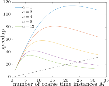
(a) Local-forecast initialization and Newton initial guesses

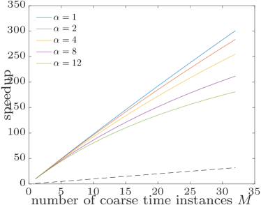
(b) Global-forecast initialization and Newton initial guesses

Fig. 14: Ideal-conditions speedup with Newton-solver initial guesses (nonlinear dynamical systems with implicit time integration). Plot corresponds to $m=5000$ fine time instances, setting the number of processors equal to the number of coarse time instances ${M}$. Note that the proposed method can realize super-ideal theoretical speedups by effectively leveraging time-evolution data.

• Proof of Corollary 15.  Under Assumptions A3 and A4, we have from Lemma 2 that ${\mathbf{h}^{{n}}}({\mathbf{r}^{T}_{j}}{\mathbf{x}})\in\mathrm{Ran}(\mathbf{\Xi}_{j}^{{n}})$, $j\in{\rm Nature}{N}$, ${{n}}\in\mathbb{N}_{0}({M}-1)$. Under Assumptions A3, A4, A5, and A6, we have from Theorem 6 that convergence occurs in one parareal iteration (i.e., ${K}=0$ in Algorithm 1).

  Then, the local forecast for the $j$th element of the restricted state to time $t^{i}\in\mathcal{t}^{{{n}}}$ during Step 2 in Algorithm 1 satisfies

  (83) $$\begin{split}{f}_{j}^{{n}}({\mathbf{r}^{T}_{j}}\mathcal{f}^{{{n}}}({\mathbf{x}}^{{{n}}}_{0});{T}^{{{n}}},t^{i})&={f}_{j}^{{n}}({\mathbf{r}^{T}_{j}}\mathcal{f}^{{{n}}}({\mathbf{x}}({T}^{{{n}}}));{T}^{{{n}}},t^{i})={f}_{j}^{{n}}({\mathbf{r}^{T}_{j}}{\mathbf{x}};{T}^{{{n}}},t^{i})\\ &={\mathbf{r}^{T}_{j}}{\mathbf{x}}({T}^{{{n}}})+\mathbf{e}_{i-{{{\bar{m}}}}{{n}}}^{T}\mathbf{\Xi}_{j}^{{n}}[{{\mathbf{Z}}_{0}}\mathbf{\Xi}_{j}^{{n}}]^{+}{{\mathbf{Z}}_{0}}{\mathbf{h}^{{n}}}({\mathbf{r}^{T}_{j}}{\mathbf{x}})\\ &={\mathbf{r}^{T}_{j}}{\mathbf{x}}({T}^{{{n}}})+\mathbf{e}_{i-{{{\bar{m}}}}{{n}}}^{T}\mathbf{\Xi}_{j}^{{n}}\hat{\hat{\mathbf{r}}}_{j}^{{{n}}}={\mathbf{r}^{T}_{j}}{\mathbf{x}}({T}^{{{n}}})+\mathbf{e}_{i-{{{\bar{m}}}}{{n}}}^{T}{\mathbf{h}^{{n}}}({\mathbf{r}^{T}_{j}}{\mathbf{x}})={\mathbf{r}^{T}_{j}}{\mathbf{x}}(t^{i}).\end{split}$$

  Under Assumptions A16 and A17, the residual arising at each time step is nonlinear and satisfies $\mathbf{r}^{i}({\mathbf{x}}(t^{i}))=0$, $i\in{\rm Nature}{m}$. Under Assumption A18, a local forecast (83) is employed as an initial guess for Newton’s method for solving $\mathbf{r}^{i}(\mathbf{w})=0$ with $t^{i}\in\mathcal{t}^{{{n}}}$ at parareal iteration ${k}$; this initial guess can be expressed as

  $$\mathbf{w}^{i,(0)} ={\mathbf{P}}[{f}_{1}^{{n}}({\mathbf{r}^{T}_{j}}\mathcal{f}^{{{n}}}({\mathbf{x}}^{{{n}}}_{0});{T}^{{{n}}},t^{i})\ \cdots\ {f}_{N}^{{n}}({\mathbf{r}^{T}_{j}}\mathcal{f}^{{{n}}}({\mathbf{x}}^{{{n}}}_{0});{T}^{{{n}}},t^{i})]^{T}$$

  $$={\mathbf{P}}[{\mathbf{r}^{T}_{1}}{\mathbf{x}}(t^{i})\ \cdots\ {\mathbf{r}^{T}_{N}}{\mathbf{x}}(t^{i})]^{T}={\mathbf{x}}(t^{i}).$$

  Because $\mathbf{r}^{i}(\mathbf{w}^{i,(0)})=\mathbf{r}^{i}({\mathbf{x}}(t^{i}))=0$ under the stated assumptions, the initial residual is zero such that Newton’s method terminates after simply computing the initial residual. No Newton iterations are required.

  Under Assumption A8, the wall time incurred by the serial solution is $m\tau_{\mathcal{F}}$, where $\tau_{\mathcal{F}}$ in this case corresponds to solving a system of nonlinear algebraic equations. The wall time incurred by the proposed approach is composed of (1) the serial coarse propagation in Step 2 of Algorithm 1, which entails solving $\alpha$ systems of nonlinear algebraic equations in each time interval (i.e., $({M}-1)\alpha\tau_{\mathcal{F}}$) and (2) the (worst-case) parallel fine propagation in Steps 3–5, which no longer requires solving systems of nonlinear algebraic equations; it entails computing only a single residual for each remaining time instance (i.e., $({\bar{m}}-\alpha)\tau_{r}\tau_{\mathcal{F}}$). The ratio of these costs yields the theoretical speedup. Again, additional speedups may be realizable by pipelining operations. $\blacksquare$

• Proof of Corollary 16.  Under Assumptions A3, A5, and A7, we have from Theorem 7 that ${\mathbf{h}}({\mathbf{r}^{T}_{j}}{\mathbf{x}})=\mathbf{\Xi}_{j}\hat{\mathbf{r}}_{j}$ for some $\hat{\mathbf{r}}_{j}\in\mathbb{R}^{{a}}$ (see Eq. (65)) and convergence in one parareal iteration (i.e., ${K}=0$ in Algorithm 1). Then, the global forecast for the $j$th element of the restricted state to time $t^{i}\in\mathcal{t}$ during Step 2 in Algorithm 1 satisfies (from Eqs. (6) and (8))

  (84) $$\begin{split}{f}_{j}({\mathbf{r}^{T}_{j}}\mathcal{f}({\mathbf{x}}^{0});0,t^{i})={f}_{j}({\mathbf{r}^{T}_{j}}{\mathbf{x}};0,t^{i})&={\mathbf{r}^{T}_{j}}{\mathbf{x}}(0)+\mathbf{e}_{i}^{T}\mathbf{\Xi}_{j}[{{\mathbf{Z}}_{0}}\mathbf{\Xi}_{j}]^{+}{{\mathbf{Z}}_{0}}\mathbf{\Xi}_{j}\hat{\mathbf{r}}_{j}={\mathbf{r}^{T}_{j}}{\mathbf{x}}(0)+\mathbf{e}_{i}^{T}\mathbf{\Xi}_{j}\hat{\mathbf{r}}_{j}\\ &={\mathbf{r}^{T}_{j}}{\mathbf{x}}(0)+\mathbf{e}_{i}^{T}{\mathbf{h}}({\mathbf{r}^{T}_{j}}{\mathbf{x}})={\mathbf{r}^{T}_{j}}{\mathbf{x}}(t^{i}).\end{split}$$

  Under Assumptions A16 and A17, the residual arising at each time step is nonlinear and satisfies $\mathbf{r}^{i}({\mathbf{x}}(t^{i}))=0$, $i\in{\rm Nature}{m}$. Under Assumption A19, global forecast (84) is employed as an initial guess for Newton’s method for solving $\mathbf{r}^{i}(\mathbf{w})=0$ with $t^{i}\in\mathcal{t}^{{{n}}}$ at all parareal iterations. This initial guess can be written as

  $$\mathbf{w}^{i,(0)}={\mathbf{P}}[{f}_{1}({\mathbf{r}^{T}_{1}}\mathcal{f}({\mathbf{x}}^{0});0,t^{i})\ \cdots\ {f}_{N}({\mathbf{r}^{T}_{N}}\mathcal{f}({\mathbf{x}}^{0});0,t^{i})]^{T}={\mathbf{P}}[{\mathbf{r}^{T}_{1}}{\mathbf{x}}(t^{i})\ \cdots\ {\mathbf{r}^{T}_{N}}{\mathbf{x}}(t^{i})]^{T}={\mathbf{x}}(t^{i}).$$

  Because $\mathbf{r}^{i}(\mathbf{w}^{i,(0)})=\mathbf{r}^{i}({\mathbf{x}}(t^{i}))=0$ under the stated assumptions, the initial residual is zero so that Newton’s method terminates after simply computing the initial residual without any required Newton iterations.

  Under Assumption A8, the wall time incurred by the serial solution is $m\tau_{\mathcal{F}}$, where $\tau_{\mathcal{F}}$ in this case corresponds to solving a system of nonlinear algebraic equations. The wall time incurred by the proposed forecasting approach is composed of (1) solving $\alpha$ systems of nonlinear algebraic equations in the first coarse time interval for initialization in Step 2 of Algorithm 1 (i.e., $\alpha\tau_{\mathcal{F}}$) and (2) the worst-case parallel fine propagation in Steps 3–5, which no longer requires solving any linear algebraic systems of equations; it entails computing only a single residual for all remaining time instances (i.e., ${\bar{m}}\tau_{r}\tau_{\mathcal{F}}$). The ratio of these costs yields the theoretical speedup. $\blacksquare$

Thus, the method realizes super-ideal speedups when the local-forecast is applied to Newton-solver initial guesses in the nonlinear case (Corollaries 15–16 and Figure 14)

References

- [1] A. Axelsson and J. Verwer, Boundary value techniques for initial value problems in ordinary differential equations, mathematics of computation, 45 (1985), pp. 153–171.
- [2] L. Baffico, S. Bernard, Y. Maday, G. Turinici, and G. Zérah, Parallel-in-time molecular-dynamics simulations, Physical Review E, 66 (2002), p. 057701.
- [3] G. Bal, On the convergence and the stability of the parareal algorithm to solve partial differential equations, in Domain Decomposition Methods in Science and Engineering, Springer, 2005, pp. 425–432.
- [4] G. Bal and Y. Maday, A “parareal” time discretization for non-linear PDEs with application to the pricing of an American put, in Recent developments in domain decomposition methods, Springer, 2002, pp. 189–202.
- [5] M. Barrault, Y. Maday, N. C. Nguyen, and A. T. Patera, An ‘empirical interpolation’ method: application to efficient reduced-basis discretization of partial differential equations, Comptes Rendus Mathématique Académie des Sciences, 339 (2004), pp. 667–672.
- [6] A. Bellen and M. Zennaro, Parallel algorithms for initial-value problems for difference and differential equations, Journal of Computational and applied mathematics, 25 (1989), pp. 341–350.
- [7] A. Blouza, L. Boudin, and S. M. Kaber, Parallel in time algorithms with reduction methods for solving chemical kinetics, Communications in Applied Mathematics and Computational Science, 5 (2011), pp. 241–263.
- [8] K. Carlberg, Model Reduction of Nonlinear Mechanical Systems via Optimal Projection and Tensor Approximation, PhD thesis, Stanford University, 2011.
- [9] K. Carlberg, M. Barone, and H. Antil, Galerkin v. least-squares Petrov–Galerkin projection in nonlinear model reduction, Journal of Computational Physics, 330 (2017), pp. 693–734.
- [10] K. Carlberg, C. Farhat, and C. Bou-Mosleh, Efficient non-linear model reduction via a least-squares Petrov–Galerkin projection and compressive tensor approximations, International Journal for Numerical Methods in Engineering, 86 (2011), pp. 155–181.
- [11] K. Carlberg, C. Farhat, J. Cortial, and D. Amsallem, The GNAT method for nonlinear model reduction: effective implementation and application to computational fluid dynamics and turbulent flows, Journal of Computational Physics, 242 (2013), pp. 623–647.
- [12] K. Carlberg, J. Ray, and B. van Bloemen Waanders, Decreasing the temporal complexity for nonlinear, implicit reduced-order models by forecasting, Computer Methods in Applied Mechanics and Engineering, 289 (2015), pp. 79–103.
- [13] S. Chaturantabut and D. C. Sorensen, Nonlinear model reduction via discrete empirical interpolation, SIAM Journal on Scientific Computing, 32 (2010), pp. 2737–2764.
- [14] F. Chen, J. S. Hesthaven, and X. Zhu, On the use of reduced basis methods to accelerate and stabilize the parareal method, in Reduced Order Methods for Modeling and Computational Reduction, Springer, 2014, pp. 187–214.
- [15] Y. Choi and K. Carlberg, Space–time least-squares Petrov–Galerkin projection for nonlinear model reduction, arXiv preprint arXiv:1703.04560, (2017).
- [16] J. Cortial, Time-parallel methods for accelerating the solution of structural dynamics problems, PhD thesis, Stanford University, 2011.
- [17] J. Cortial and C. Farhat, A time-parallel implicit method for accelerating the solution of non-linear structural dynamics problems, International Journal for Numerical Methods in Engineering, 77 (2009), pp. 451–470.
- [18] M. Drohmann, B. Haasdonk, and M. Ohlberger, Reduced basis approximation for nonlinear parametrized evolution equations based on empirical operator interpolation, SIAM Journal on Scientific Computing, 34 (2012), pp. A937–A969.
- [19] M. Emmett and M. Minion, Toward an efficient parallel in time method for partial differential equations, Communications in Applied Mathematics and Computational Science, 7 (2012), pp. 105–132.
- [20] S. Engblom, Parallel in time simulation of multiscale stochastic chemical kinetics, Multiscale Modeling & Simulation, 8 (2009), pp. 46–68.
- [21] R. Everson and L. Sirovich, Karhunen–Loève procedure for gappy data, Journal of the Optical Society of America A, 12 (1995), pp. 1657–1664.
- [22] R. D. Falgout, S. Freidhoff, T. V. Kolev, S. P. MacLachlan, and J. B. Schroder, Parallel time integration with multigrid, SIAM J. Sci. Comput., 36 (2014), pp. C635–C661.
- [23] C. Farhat and M. Chandesris, Time-decomposed parallel time-integrators: theory and feasibility studies for fluid, structure, and fluid–structure applications, International Journal for Numerical Methods in Engineering, 58 (2003), pp. 1397–1434.
- [24] C. Farhat, J. Cortial, C. Dastillung, and H. Bavestrello, Time-parallel implicit integrators for the near-real-time prediction of linear structural dynamic responses, International Journal for Numerical Methods in Engineering, 67 (2006), pp. 697–724.
- [25] P. F. Fischer, F. Hecht, and Y. Maday, A parareal in time semi-implicit approximation of the Navier-Stokes equations, in Domain decomposition methods in science and engineering, Springer, 2005, pp. 433–440.
- [26] M. J. Gander, Overlapping Schwarz for parabolic problems, in Proc. of Ninth International Conference on Domain Decomposition Methods, 1998.
- [27] M. J. Gander, 50 years of time parallel time integration, in Multiple Shooting and Time Domain Decomposition Methods, Springer, 2015, pp. 69–113.
- [28] M. J. Gander and E. Hairer, Nonlinear convergence analysis for the parareal algorithm, in Domain decomposition methods in science and engineering XVII, Springer, 2008, pp. 45–56.
- [29] M. J. Gander and S. Vandewalle, Analysis of the parareal time-parallel time-integration method, SIAM Journal on Scientific Computing, 29 (2007), pp. 556–578.
- [30] D. Guibert and D. Tromeur-Dervout, Adaptive parareal for systems of ODEs, in Domain decomposition methods in science and engineering XVI, Springer, 2007, pp. 587–594.
- [31] W. Hackbusch, Parabolic multi-grid methods, in Computing Methods in Applied Sciences and Engineering, R. Glowinski, VI and J. Lions, eds., North-Holland, 1984, pp. 189–197.
- [32] G. Horton and S. Vandewalle, A space-time multigrid method for parabolic partial differential equations, SIAM Journal on Scientific Computing, 16 (1995), pp. 848–864.
- [33] J. Lions, Y. Maday, and G. Turinici, A”parareal”in time discretization of PDE’s, Comptes Rendus de l’Academie des Sciences Series I Mathematics, 332 (2001), pp. 661–668.
- [34] C. Lubich and A. Ostermann, Multi-grid dynamic iteration for parabolic equations, BIT Numerical Mathematics, 27 (1987), pp. 216–234.
- [35] Y. Maday, Parareal in time algorithm for kinetic systems based on model reduction, High-dimensional partial differential equations in science and engineering, 41 (2007), pp. 183–194.
- [36] Y. Maday and E. M. Rønquist, Parallelization in time through tensor-product space–time solvers, Comptes Rendus Mathematique, 346 (2008), pp. 113–118.
- [37] Y. Maday and G. Turinici, Parallel in time algorithms for quantum control: Parareal time discretization scheme, International journal of quantum chemistry, 93 (2003), pp. 223–228.
- [38] M. Minion, A hybrid parareal spectral deferred corrections method, Communications in Applied Mathematics and Computational Science, 5 (2011), pp. 265–301.
- [39] W. L. Miranker and W. Liniger, Parallel methods for the numerical integration of ordinary differential equations, Mathematics of Computation, 21 (1967), pp. 303–320.
- [40] M. Neumüller, Space-time methods: Fast Solvers and Applications, PhD thesis, University of Graz, 2013.
- [41] A. S. Nielsen, Feasibility study of the parareal algorithm, masters thesis, Technical University of Denmark, DTU Informatic, 2012.
- [42] J. Nievergelt, Parallel methods for integrating ordinary differential equations, Communications of the ACM, 7 (1964), pp. 731–733.
- [43] M. J. Rewienski, A Trajectory Piecewise-Linear Approach to Model Order Reduction of Nonlinear Dynamical Systems, PhD thesis, Massachusetts Institute of Technology, 2003.
- [44] D. Ruprecht and R. Krause, Explicit parallel-in-time integration of a linear acoustic-advection system, Computers & Fluids, 59 (2012), pp. 72–83.
- [45] P. Saha, J. Stadel, and S. Tremaine, A parallel integration method for solar system dynamics, The Astronomical Journal, 114 (1997), p. 409.
- [46] D. Sheen, I. H. Sloan, and V. Thomée, A parallel method for time discretization of parabolic equations based on Laplace transformation and quadrature, IMA Journal of Numerical Analysis, 23 (2003), pp. 269–299.
- [47] D. A. D. Subcommittee, Synergistic challenges in data-intensive science and exascale computing, DOE Office of Science, (2013).
- [48] S. Vandewalle, Parallel multigrid waveform relaxation for parabolic problems, Springer-Verlag, 2013.
- [49] N. Vannieuwenhoven, R. Vandebril, and K. Meerbergen, A new truncation strategy for the higher-order singular value decomposition, SIAM Journal on Scientific Computing, 34 (2012), pp. A1027–A1052.
- [50] D. E. Womble, A time-stepping algorithm for parallel computers, SIAM Journal on Scientific and Statistical Computing, 11 (1990), pp. 824—837.
- [51] P. Worley, Parallelizing across time when solving time-dependent partial differential equations, in Proc. 5th SIAM Conf. on Parallel Processing for Scientific Computing, D. Sorensen, ed., SIAM, 1991.