11institutetext: Vincent Brault 22institutetext: Univ. Grenoble Alpes, Inria, CNRS, Grenoble INP111Institute of Engineering Univ. Grenoble Alpes, LJK, 38000 Grenoble, France
22email: vincent.brault@univ-grenoble-alpes.fr
33institutetext: Antoine Channarond 44institutetext: UMR6085 CNRS, Laboratoire de Mathématiques Raphaël Salem, Université de Rouen Normandie, 76800 Saint-Étienne-du-Rouvray, France
44email: antoine.channarond@univ-rouen.fr

Fast and Consistent Algorithm for the Latent Block Modelthanks: Thanks to Stéphane Robin and the reviewers for them suggestions. This work has been partially supported by the LabEx PERSYVAL-Lab (ANR-11-LABX-0025-01) funded by the French program Investissement d’avenir and partially supported by MIAI@Grenoble Alpes (ANR-19-P3IA-0003). All the computations presented in this paper were performed using the GRICAD infrastructure (https://gricad.univ-grenoble-alpes.fr), which is supported by Grenoble research communities.

Vincent Brault    Antoine Channarond
(Received: date / Accepted: date)
Abstract

The latent block model is used to simultaneously rank the rows and columns of a matrix to reveal a block structure. The algorithms used for estimation are often time consuming. However, recent work shows that the log-likelihood ratios are equivalent under the complete and observed (with unknown labels) models and the groups posterior distribution to converge as the size of the data increases to a Dirac mass located at the actual groups configuration. Based on these observations, the algorithm Largest Gaps is proposed in this paper to perform clustering using only the marginals of the matrix, when the number of blocks is very small with respect to the size of the whole matrix in the case of binary data. In addition, a model selection method is incorporated with a proof of its consistency. Thus, this paper shows that studying simplistic configurations (few blocks compared to the size of the matrix or very contrasting blocks) with complex algorithms is useless since the marginals already give very good parameter and classification estimates.

Keywords:
Latent Block Model Largest Gaps Algorithm Model Selection Data analysis
MSC:

62H30 62-07 60K35

1 Introduction

Block clustering methods aim at clustering rows and columns of a matrix simultaneously to form homogeneous blocks. There are a lot of applications of this method: genomics (hedenfalk2001gene, ; jagalur2007analyzing, ), recommender systems (bennett2007netflix, ; shan2008bayesian, ), archeology (govaert1983classification, ), sociology (hartigan1975Clustering, ; keribin2014estimation, ; wyse2010block, ) or network (barbillon2017stochastic, ; bouveyron2018stochastic, ) for example. Among the methods proposed to solve this question, the Latent Block Model (LBM) (govaert2003clustering, ) provides a chessboard structure induced by the classification of the rows and the classification of the columns. In this model, it is assumed that a sample of n𝑛n individuals is collected, which contains the observation of d𝑑d binary variables of the same nature. Saying that the binary variables are of the same nature means that it is possible to encode them in the same (and natural) way. This assumption is needed to ensure that decomposing the dataset in a block structure makes sense and laclau2017co shows the equivalence between searching for a classification in the LBM and solving an optimal transport problem. In the case where the rows and columns represent the same individuals, we generally speak instead of Stochastic Block Model (barbillon2017stochastic, ; bouveyron2018stochastic, ; tabouy2020variational, ). However, in the case where the matrices are not symmetric, keribin2021cluster shows that it may be more interesting to use the LBM model rather than the SBM model. Although this model is very similar, we will not discuss it in this article.

Given the number of blocks and in order to estimate the parameters, govaert2003clustering suggest using a variational algorithm, keribin2012model propose an adaptation of the Stochastic Expectation Maximisation introduced by celeux1995stochastic in the mixture case, keribin2014estimation studied a Bayesian version of these two algorithms and wyse2010block propose a Bayesian algorithm including the estimation of the number of blocks. However, each of these iterative algorithms has a complexity at least 𝒪(ndNBlockNIter)𝒪𝑛𝑑subscript𝑁𝐵𝑙𝑜𝑐𝑘subscript𝑁𝐼𝑡𝑒𝑟\mathcal{O}\left(ndN_{Block}N_{Iter}\right) where NBlocksubscript𝑁𝐵𝑙𝑜𝑐𝑘N_{Block} is the number of blocks and NItersubscript𝑁𝐼𝑡𝑒𝑟N_{Iter} is the number of iterations necessary for the convergence of the algorithm. Moreover, the procedures are often associated with a model selection criterion requiring the computation of maximum likelihood estimators for all combinations of the expected number of blocks. However, the theoretical results obtained show that the distributions of the estimators (see brault2020consistency ; celisse2012consistency ; mariadassou2012convergence ) are asymptotically trivial: the log-likelihood ratios are equivalent under the complete and observed (with unknown labels) models and the groups posterior distribution to converge as the size of the data increases to a Dirac mass located at the actual groups configuration.

In this article, we propose an adaptation of the Largest Gaps (LG) algorithm introduced by channarond2011Classification in the Stochastic Block Model with a low complexity 𝒪(nd)𝒪𝑛𝑑\mathcal{O}(nd) (Section 3) and present the conditions to obtain asymptotically a good estimation (Section 4). We then prove that it provides a consistent procedure for all inference tasks inherent in LBM: unsupervised classification and estimation of the parameters and a selection procedure for the number of blocks (the last unknown theoretical point) is also proposed and shown to be consistent (Section 5.3). For ease of reading, the proofs of the results are postponed to the appendices (Sections A, B and C). These theoretical results are also illustrated on simulated data (Section 6).

By proving the consistency of the LG algorithm, some features of the asymptotic regime of the LBM will be highlighted, in particular, the concentration of some marginal distributions of the model. The secondary objective of the paper is to discuss as a conclusion (Section 7) the consequence of this when fitting the LBM to large matrices; in particular, this leads to take a step back regarding the relevance of the model and the estimates when the number of blocks is small with respect to the number of cells of the matrix.

2 Notations and model

The binary Latent Block Model (LBM) is as follows. Let 𝐱=(xij)i=1,,n;j=1,,d𝐱subscriptsubscript𝑥𝑖𝑗formulae-sequence𝑖1𝑛𝑗1𝑑\mathbf{x}=\left(x_{ij}\right)_{i=1,\ldots,n;j=1,\ldots,d} be the data matrix where xij{0,1}subscript𝑥𝑖𝑗01x_{ij}\in\{0,1\}; observation of a random variable 𝐗𝐗\mathbf{X}. It is assumed that there exists a partition into g𝑔g row clusters 𝐳=(zik)i=1,,n;k=1,,g𝐳subscriptsubscript𝑧𝑖𝑘formulae-sequence𝑖1𝑛𝑘1𝑔\mathbf{z}=\left(z_{ik}\right)_{i=1,\ldots,n;k=1,\ldots,g} and a partition into m𝑚m column clusters 𝐰=(wj)j=1,,d;=1,,m𝐰subscriptsubscript𝑤𝑗formulae-sequence𝑗1𝑑1𝑚\mathbf{w}=\left(w_{j\ell}\right)_{j=1,\ldots,d;\ell=1,\ldots,m}. The ziksubscript𝑧𝑖𝑘z_{ik}s (resp. wjsubscript𝑤𝑗w_{j\ell}s ) are binary indicators of row i𝑖i (resp. column j𝑗j) belonging to row cluster k𝑘k (resp. column cluster \ell), such that the random variables Xijsubscript𝑋𝑖𝑗X_{ij} are independent conditionally on 𝐳𝐳\mathbf{z} and 𝐰𝐰\mathbf{w} with parametric density φ(;αk)zikwj𝜑superscriptsubscript𝛼𝑘subscript𝑧𝑖𝑘subscript𝑤𝑗\varphi(\cdot;\alpha_{k\ell})^{z_{ik}w_{j\ell}}, where αksubscript𝛼𝑘\alpha_{k\ell} is the parameter of the conditional density of the data given Zik=1subscript𝑍𝑖𝑘1Z_{ik}=1 and Wj=1subscript𝑊𝑗1W_{j\ell}=1. As the binary case is studied, the density is defined for each x{0,1}𝑥01x\in\{0,1\} and α[0;1]𝛼01\alpha\in[0;1] by

φ(x;α)=αx(1α)1x.𝜑𝑥𝛼superscript𝛼𝑥superscript1𝛼1𝑥\varphi(x;\alpha)=\alpha^{x}\left(1-\alpha\right)^{1-x}.

Thus, the density of 𝐗𝐗\mathbf{X} conditionally on 𝐳𝐳\mathbf{z} and 𝐰𝐰\mathbf{w} is defined for each 𝐱𝐱\mathbf{x} by

f(𝐱|𝐳,𝐰;𝜶)𝑓conditional𝐱𝐳𝐰𝜶\displaystyle f(\mathbf{x}|\mathbf{z},\mathbf{w};\boldsymbol{\alpha}) =\displaystyle= i=1nj=1dk=1g=1mφ(xij;αk)zikwjsuperscriptsubscriptproduct𝑖1𝑛superscriptsubscriptproduct𝑗1𝑑superscriptsubscriptproduct𝑘1𝑔superscriptsubscriptproduct1𝑚𝜑superscriptsubscript𝑥𝑖𝑗subscript𝛼𝑘subscript𝑧𝑖𝑘subscript𝑤𝑗\displaystyle\prod_{i=1}^{n}\prod_{j=1}^{d}\prod_{k=1}^{g}\prod_{\ell=1}^{m}\varphi(x_{ij};\alpha_{k\ell})^{z_{ik}w_{j\ell}}
=:absent:\displaystyle=: i,j,k,φ(xij;αk)zikwjsubscriptproduct𝑖𝑗𝑘𝜑superscriptsubscript𝑥𝑖𝑗subscript𝛼𝑘subscript𝑧𝑖𝑘subscript𝑤𝑗\displaystyle\prod_{i,j,k,\ell}\varphi(x_{ij};\alpha_{k\ell})^{z_{ik}w_{j\ell}}

where 𝜶=(αk)k=1,,g;=1,,m𝜶subscriptsubscript𝛼𝑘formulae-sequence𝑘1𝑔1𝑚\boldsymbol{\alpha}=\left(\alpha_{k\ell}\right)_{k=1,\ldots,g;\ell=1,\ldots,m}.

Moreover, it is assumed that the row and column labels 𝐳𝐳\mathbf{z} and 𝐰𝐰\mathbf{w} are the observations of two independent variables 𝐙𝐙\mathbf{Z} and 𝐖𝐖\mathbf{W}: p(𝐳,𝐰;𝝅,𝝆)=p(𝐳;𝝅)p(𝐰;𝝆)𝑝𝐳𝐰𝝅𝝆𝑝𝐳𝝅𝑝𝐰𝝆p(\mathbf{z},\mathbf{w};\boldsymbol{\pi},\boldsymbol{\rho})=p(\mathbf{z};\boldsymbol{\pi})p(\mathbf{w};\boldsymbol{\rho}) with p(𝐳;𝝅)=i,kπkzik=kπkz+k𝑝𝐳𝝅subscriptproduct𝑖𝑘superscriptsubscript𝜋𝑘subscript𝑧𝑖𝑘subscriptproduct𝑘superscriptsubscript𝜋𝑘subscript𝑧𝑘p(\mathbf{z};\boldsymbol{\pi})=\prod_{i,k}\pi_{k}^{z_{ik}}=\prod_{\scriptscriptstyle k}\pi_{k}^{z_{+k}} and p(𝐰;𝝆)=j,ρwj=ρw+𝑝𝐰𝝆subscriptproduct𝑗superscriptsubscript𝜌subscript𝑤𝑗subscriptproductsuperscriptsubscript𝜌subscript𝑤p(\mathbf{w};\boldsymbol{\rho})=\prod_{j,\ell}\rho_{\ell}^{w_{j\ell}}=\prod_{\scriptscriptstyle\ell}\rho_{\ell}^{w_{+\ell}}, where (πk=(Zik=1),k=1,,g)formulae-sequencesubscript𝜋𝑘subscript𝑍𝑖𝑘1𝑘1𝑔(\pi_{k}=\mathbb{P}(Z_{ik}=1),k=1,\ldots,g) and (ρ=(Wj=1),=1,,m)formulae-sequencesubscript𝜌subscript𝑊𝑗11𝑚(\rho_{\ell}=\mathbb{P}(W_{j\ell}=1),\ell=1,\ldots,m) are the mixing proportions and z+k=i=1nziksubscript𝑧𝑘superscriptsubscript𝑖1𝑛subscript𝑧𝑖𝑘z_{+k}=\sum_{i=1}^{n}{z_{ik}} (resp. w+=j=1dwjsubscript𝑤superscriptsubscript𝑗1𝑑subscript𝑤𝑗w_{+\ell}=\sum_{j=1}^{d}{w_{j\ell}}) represents the number of rows (resp. columns) in the class k𝑘k (resp. \ell). Hence, the density of 𝐗𝐗\mathbf{X} is defined for every 𝐱𝐱\mathbf{x} by

f(𝐱;𝜽)=(𝐳,𝐰)𝒵×𝒲p(𝐳;𝝅)p(𝐰;𝝆)f(𝐱|𝐳,𝐰;𝜶),𝑓𝐱𝜽subscript𝐳𝐰𝒵𝒲𝑝𝐳𝝅𝑝𝐰𝝆𝑓conditional𝐱𝐳𝐰𝜶f(\mathbf{x};\boldsymbol{\theta})=\sum_{(\mathbf{z},\mathbf{w})\in\mathcal{Z}\times\mathcal{W}}p(\mathbf{z};\boldsymbol{\pi})p(\mathbf{w};\boldsymbol{\rho})f(\mathbf{x}|\mathbf{z},\mathbf{w};\boldsymbol{\alpha}),

where 𝒵𝒵\mathcal{Z} and 𝒲𝒲\cal W denoting the sets of all possible row labels 𝐳𝐳\mathbf{z} and column labels 𝐰𝐰\mathbf{w}, and 𝜽=(𝝅,𝝆,𝜶)𝜽𝝅𝝆𝜶\boldsymbol{\theta}=(\boldsymbol{\pi},\boldsymbol{\rho},\boldsymbol{\alpha}), with 𝝅=(π1,,πg)𝝅subscript𝜋1subscript𝜋𝑔\boldsymbol{\pi}=(\pi_{1},\ldots,\pi_{g}) and 𝝆=(ρ1,,ρm)𝝆subscript𝜌1subscript𝜌𝑚\boldsymbol{\rho}=(\rho_{1},\ldots,\rho_{m}). The density of 𝐗𝐗\mathbf{X} can be written for every 𝐱𝐱\mathbf{x} as

f(𝐱;𝜽)𝑓𝐱𝜽\displaystyle f(\mathbf{x};\boldsymbol{\theta}) =\displaystyle= (𝐳,𝐰)𝒵×𝒲kπkz+kρw+i,j,k,φ(xij;αk)zikwj.subscript𝐳𝐰𝒵𝒲subscriptproduct𝑘superscriptsubscript𝜋𝑘subscript𝑧𝑘subscriptproductsuperscriptsubscript𝜌subscript𝑤subscriptproduct𝑖𝑗𝑘𝜑superscriptsubscript𝑥𝑖𝑗subscript𝛼𝑘subscript𝑧𝑖𝑘subscript𝑤𝑗\displaystyle\sum_{(\mathbf{z},\mathbf{w})\in\mathcal{Z}\times\mathcal{W}}\prod_{\scriptscriptstyle k}\pi_{k}^{z_{+k}}\prod_{\scriptscriptstyle\ell}\rho_{\ell}^{w_{+\ell}}\!\prod_{\scriptscriptstyle i,j,k,\ell}\varphi(x_{ij};\alpha_{k\ell})^{z_{ik}w_{j\ell}}.

To estimate both the classification and the parameters, many algorithms exist (for example govaert2003clustering , keribin2014estimation or wyse2010block ) but each of these algorithms has a complexity larger than 𝒪(ndgmNIter)𝒪𝑛𝑑𝑔𝑚subscript𝑁𝐼𝑡𝑒𝑟\mathcal{O}\left(ndgmN_{Iter}\right) where NItersubscript𝑁𝐼𝑡𝑒𝑟N_{Iter} is the number of iterations of the algorithm. This makes their use on large matrices difficult.

In the Stochastic Block Model (SBM), rows and columns are associated with the same individuals, which allows to represent a graph, whereas LBM allows to represent bipartite graphs. channarond2011Classification suggested a fast algorithm, called LG𝐿𝐺LG for Lagest Gaps, based on a marginal of the matrix 𝐱𝐱\mathbf{x}, the degrees.

3 Algorithm Largest Gaps

Before the introduction of the classification algorithm Largest Gaps (LG𝐿𝐺LG), let us recall the main idea, inspired by channarond2011Classification .

3.1 Main ideas

Conditionally on Zik=1subscript𝑍𝑖𝑘1Z_{ik}=1, meaning that row i𝑖i is in class k𝑘k, the probability that the variable Xijsubscript𝑋𝑖𝑗X_{ij} equals 111 for any j{1,,d}𝑗1𝑑j\in\{1,\ldots,d\} is

(Xij=1|Zik=1)subscript𝑋𝑖𝑗conditional1subscript𝑍𝑖𝑘1\displaystyle\mathbb{P}\left(X_{ij}=1|Z_{ik}=1\right) =\displaystyle= =1m(Xij=1|Zik=1,Wj=1)(Wj=1|Zik=1)\displaystyle\sum_{\ell=1}^{m}\mathbb{P}\left(X_{ij}=1|Z_{ik}=1,W_{j\ell}=1\right)\mathbb{P}\left(W_{j\ell}=1|Z_{ik}=1\right) (1)
=\displaystyle= =1m(Xij=1|Zik=1,Wj=1)(Wj=1)\displaystyle\sum_{\ell=1}^{m}\mathbb{P}\left(X_{ij}=1|Z_{ik}=1,W_{j\ell}=1\right)\mathbb{P}\left(W_{j\ell}=1\right)
=\displaystyle= =1mαkρ=:τk.\displaystyle\sum_{\ell=1}^{m}\alpha_{k\ell}\rho_{\ell}=:\tau_{k}.

In particular, conditionally on Zik=1subscript𝑍𝑖𝑘1Z_{ik}=1, variables of row i𝑖i are independent and identically distributed Bernoulli variables with parameter τksubscript𝜏𝑘\tau_{k} and the sum of the cells of any row i𝑖i, denoted by Xi+subscript𝑋limit-from𝑖X_{i+}, is hence a binomial distributed variable in(d,τk)𝑖𝑛𝑑subscript𝜏𝑘\mathcal{B}in\left(d,\tau_{k}\right).

As a consequence of the subgaussian concentration property of binomial distributions, variables Xi¯=Xi+d¯subscript𝑋𝑖subscript𝑋limit-from𝑖𝑑\overline{X_{i\centerdot}}=\frac{X_{i+}}{d} fastly concentrates around the mean associated with its own class when d𝑑d tend to infinity. The point is here: if moreover these means τ1,,τgsubscript𝜏1subscript𝜏𝑔\tau_{1},\ldots,\tau_{g} are pairwise distinct, the set of the variables {Xi¯;i=1,,n}formulae-sequence¯subscript𝑋𝑖𝑖1𝑛\{\overline{X_{i\centerdot}};i=1,\dots,n\} asymptotically splits into clusters, separated by large gaps, and which exactly correspond to the clusters of the model, for d𝑑d large enough. In the whole paper, τ1,,τgsubscript𝜏1subscript𝜏𝑔\tau_{1},\ldots,\tau_{g} will be assumed to be pairwise distinct (Assumption (1), see discussion in Section 4).

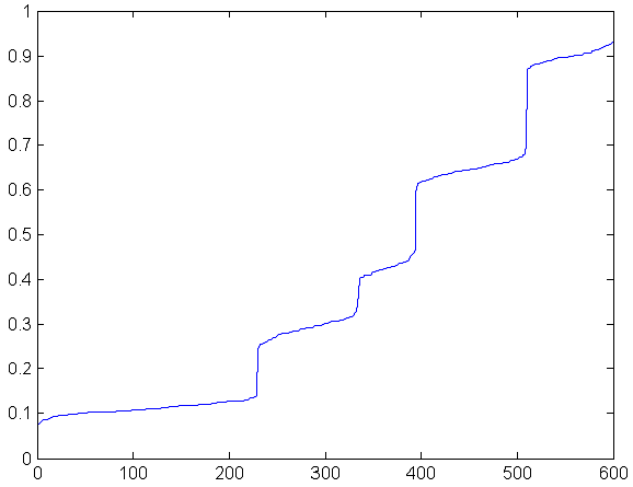
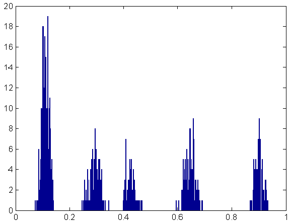
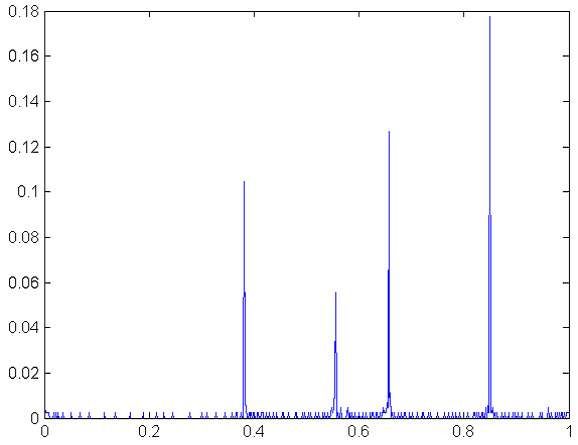
The middle right picture of Figure 1 shows the histogram of the variable set {Xi¯;i=1,,n}formulae-sequence¯subscript𝑋𝑖𝑖1𝑛\{\overline{X_{i\centerdot}};i=1,\dots,n\} for a matrix simulated under LBM with five clusters. The five clusters of rows can be seen, as well as the four large gaps which separate them. The middle left picture of Figure 1 is a representation of the vector (Xi¯(\overline{X_{i\centerdot}} sorted in ascending order and the bottom left picture of Figure 1, the size of the gaps between two consecutive sorted values.

To classify the rows, the idea is to identify the gaps between the clusters, which are expected to be asymptotically larger. Indeed, the internal gaps (those between two rows of the same cluster) vanish when d𝑑d tends to infinity due to concentration, while the external gaps (those between two rows of distinct clusters) do not, since the means are assumed to be distinct. Symmetrically the same holds for the columns.

There are several strategies to identify the large gaps. In their article, channarond2011Classification assume that the number Q𝑄Q of clusters (the same for the rows and the columns) is known and partition the population into Q𝑄Q clusters by finding the Q1𝑄1Q-1 largest gaps. In order to choose Q𝑄Q, a model selection procedure can be firstly done separately, before the classification. The strategy chosen in this article consists in thresholding the gaps, to distinguish outer gaps from inner ones. It advantageously yields both the clusters and the numbers of clusters in only one pass.

The choice of thresholds is critical. Let’s comment on the beautiful configuration of Figure 1, where the asymptotic regime has been reached, to present the key issues. If the thresholds are too large (greater than 0.06 on that example), the thresholding step will select only some of the four outer deviations and will not distinguish the five clusters from each other. Conversely, if they are too small (less than 0.01), the thresholding step will select all four outer gaps, but also some undesirable inner gaps, and the algorithm will wrongly separate some clusters.

3.2 Algorithm

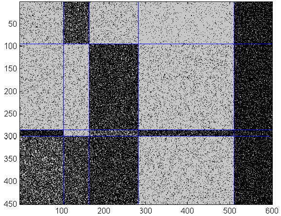
The algorithm Largest Gaps222An implementation in the language R is available on the following Gitlab: https://gricad-gitlab.univ-grenoble-alpes.fr/braultv/largest-gaps is given in Algorithm 1 and an illustration is provided in Figure 1. The principle is to calculate the means of the values of the cells of each row and each column, to order them and to calculate the differences between two consecutive values. Once this step is done, the clusters are formed assuming that each difference greater than the threshold implies a change of cluster. In the sequel, the estimators provided by the algorithm are denoted by 𝐙^^𝐙\widehat{\mathbf{Z}}, 𝐖^^𝐖\widehat{\mathbf{W}} and 𝜽^^𝜽\widehat{\boldsymbol{\theta}}.

Input: data matrix 𝐱𝐱\mathbf{x}, threshold for row Sgsubscript𝑆𝑔S_{g} and for column Smsubscript𝑆𝑚S_{m}.
// Computation of gaps
for i{1,,n}𝑖1𝑛i\in\{1,\ldots,n\} do
       Computation of Xi¯=xi+d¯subscript𝑋𝑖subscript𝑥limit-from𝑖𝑑\overline{X_{i\centerdot}}=\frac{x_{i+}}{d}.
  // 𝒪(nd)𝒪𝑛𝑑\mathcal{O}(nd)
Ascending sort of (X(1)¯,,X(n)¯)¯subscript𝑋1¯subscript𝑋𝑛\left(\overline{X_{(1)\centerdot}},\ldots,\overline{X_{(n)\centerdot}}\right).
  // 𝒪(nlogn)𝒪𝑛𝑛\mathcal{O}(n\log n)
for i{2,,n}𝑖2𝑛i\in\{2,\ldots,n\} do
       Computation of the gaps Gi=X(i)¯X(i1)¯subscript𝐺𝑖¯subscript𝑋𝑖¯subscript𝑋𝑖1G_{i}=\overline{X_{(i)\centerdot}}-\overline{X_{(i-1)\centerdot}}.
  // 𝒪(n)𝒪𝑛\mathcal{O}(n)
// Computation of g^^𝑔\widehat{g}
Selection of i1<<ig^1subscript𝑖1subscript𝑖^𝑔1i_{1}<\ldots<i_{\widehat{g}-1} such that (Gi1,,Gig^1)subscript𝐺subscript𝑖1subscript𝐺subscript𝑖^𝑔1(G_{i_{1}},\ldots,G_{i_{\widehat{g}-1}}) are every greater than Sgsubscript𝑆𝑔S_{g}.
  // 𝒪(n)𝒪𝑛\mathcal{O}(n)
// Computation of 𝐙^^𝐙\widehat{\mathbf{Z}}
for i{(1),,(n)}𝑖1𝑛i\in\{(1),\ldots,(n)\} do
       Definition of z^(i)k=1subscript^𝑧𝑖𝑘1\widehat{z}_{(i)k}=1 if and only if (ik1)<(i)(ik)subscript𝑖𝑘1𝑖subscript𝑖𝑘(i_{k-1})<(i)\leq(i_{k}) with i0=0subscript𝑖00i_{0}=0 and ig^=nsubscript𝑖^𝑔𝑛i_{\widehat{g}}=n.
  // 𝒪(n)𝒪𝑛\mathcal{O}(n)
// Computation of m^^𝑚\widehat{m} and 𝐖^^𝐖\widehat{\mathbf{W}}
Do the same on the columns.
  // 𝒪(max(dn,dlogd))𝒪𝑑𝑛𝑑𝑑\mathcal{O}(\max(dn,d\log d))
// Computation of 𝜽^^𝜽\widehat{\boldsymbol{\theta}}
for k{1,,g^}𝑘1^𝑔k\in\left\{1,\ldots,\widehat{g}\right\} do
       Computation of πk^=z^+kn^subscript𝜋𝑘subscript^𝑧𝑘𝑛\widehat{\pi_{k}}=\frac{\widehat{z}_{+k}}{n}.
  // 𝒪(n/Sg)𝒪𝑛subscript𝑆𝑔\mathcal{O}(n/S_{g})
for {1,,m^}1^𝑚\ell\in\left\{1,\ldots,\widehat{m}\right\} do
       Computation of ρ^=w^+d^subscript𝜌subscript^𝑤𝑑\widehat{\rho_{\ell}}=\frac{\widehat{w}_{+\ell}}{d}.
  // 𝒪(d/Sm)𝒪𝑑subscript𝑆𝑚\mathcal{O}(d/S_{m})
Computation of 𝜶^=(𝐙^)𝐱T𝐖^/[πk^(ρ^)]T×nd\widehat{\boldsymbol{\alpha}}=\left(\widehat{\mathbf{Z}}\right){{}^{T}}\mathbf{x}\widehat{\mathbf{W}}/\left[\widehat{\pi_{k}}\left(\widehat{\rho_{\ell}}\right){{}^{T}}\right]\times nd.
  // 𝒪(nd[1/Sg+1/Sm])𝒪𝑛𝑑delimited-[]1subscript𝑆𝑔1subscript𝑆𝑚\mathcal{O}\left(nd\left[1/S_{g}+1/S_{m}\right]\right)
Output: Numbers of clusters g^^𝑔\widehat{g} and m^^𝑚\widehat{m}, matrices 𝐙^^𝐙\widehat{\mathbf{Z}} and 𝐖^^𝐖\widehat{\mathbf{W}} and parameter 𝜽^^𝜽\widehat{\boldsymbol{\theta}}.
Algorithm 1 Algorithm Largest𝐿𝑎𝑟𝑔𝑒𝑠𝑡Largest Gaps𝐺𝑎𝑝𝑠Gaps. The complexity of each step is highlighted in blue.
Refer to caption Refer to caption
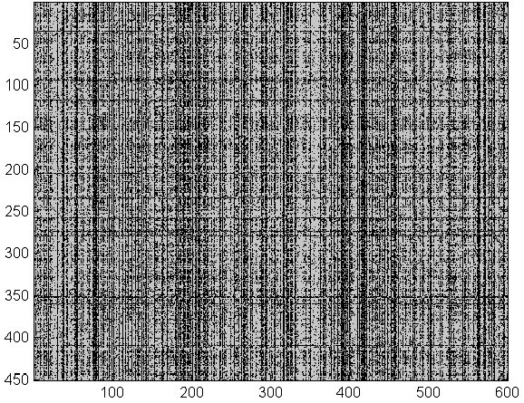
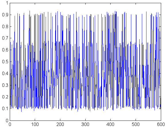
Figure 1: Top-left: Initial matrix. Top-right: Example of a vector (X(1)¯,,X(d)¯)¯subscript𝑋absent1¯subscript𝑋absent𝑑\left(\overline{X_{\centerdot(1)}},\ldots,\overline{X_{\centerdot(d)}}\right). Middle-left: representation of the vector (X(1)¯,,X(d)¯)¯subscript𝑋absent1¯subscript𝑋absent𝑑\left(\overline{X_{\centerdot(1)}},\ldots,\overline{X_{\centerdot(d)}}\right) sorted in increasing order. Middle-right: Histograms of (X(1)¯,,X(d)¯)¯subscript𝑋absent1¯subscript𝑋absent𝑑\left(\overline{X_{\centerdot(1)}},\ldots,\overline{X_{\centerdot(d)}}\right). Bottom-left: representation of the vector of gaps (G2,,Gd)subscript𝐺2subscript𝐺𝑑\left(G_{2},\ldots,G_{d}\right) where for all j{2,,d}𝑗2𝑑j\in\{2,\ldots,d\}, Gj=X(j)¯X(j1)¯subscript𝐺𝑗¯subscript𝑋absent𝑗¯subscript𝑋absent𝑗1G_{j}=\overline{X_{\centerdot(j)}}-\overline{X_{\centerdot(j-1)}}. Bottom-right: reorganized matrix.

Estimator of 𝜽superscript𝜽\boldsymbol{\theta}^{\star}.

For the rest of the article, 𝜽=(𝝅,𝝆,𝜶)superscript𝜽superscript𝝅superscript𝝆superscript𝜶\boldsymbol{\theta}^{\star}=\left(\boldsymbol{\pi}^{\star},\boldsymbol{\rho}^{\star},\boldsymbol{\alpha}^{\star}\right) represents the parameters to be estimated (i.e. the parameters that were used to simulate the data). In the algorithm 1, the estimator 𝜽^^𝜽\widehat{\boldsymbol{\theta}} of 𝜽superscript𝜽\boldsymbol{\theta}^{\star} is based on 𝐙^^𝐙\widehat{\mathbf{Z}} and 𝐖^^𝐖\widehat{\mathbf{W}}. πk^^subscript𝜋𝑘\widehat{\pi_{k}} (resp. ρ^^subscript𝜌\widehat{\rho_{\ell}}) is the proportion of class k𝑘k (resp. \ell) in the partition z^^𝑧\widehat{z} (resp. w^^𝑤\widehat{w}) and the estimator 𝜶^^𝜶\widehat{\boldsymbol{\alpha}} is for all (k,){1,,g^}×{1,,m^}𝑘1^𝑔1^𝑚\left(k,\ell\right)\in\left\{1,\ldots,\widehat{g}\right\}\times\left\{1,\ldots,\widehat{m}\right\}:

αk^=i=1nj=1dzik^wj^xijz+k^w+^.^subscript𝛼𝑘superscriptsubscript𝑖1𝑛superscriptsubscript𝑗1𝑑^subscript𝑧𝑖𝑘^subscript𝑤𝑗subscript𝑥𝑖𝑗^subscript𝑧𝑘^subscript𝑤\widehat{\alpha_{k\ell}}=\frac{\sum_{i=1}^{n}\sum_{j=1}^{d}\widehat{z_{ik}}\widehat{w_{j\ell}}x_{ij}}{\widehat{z_{+k}}\widehat{w_{+\ell}}}.

Complexity of the algorithm.

On algorithm 1, the complexities of each step are added in blue at the end of the line. In the end, the LG algorithm has a complexity of 𝒪(max(nd[g^+m^],nlogn,dlogd))𝒪𝑛𝑑delimited-[]^𝑔^𝑚𝑛𝑛𝑑𝑑\mathcal{O}\left(\max\left(nd\left[\widehat{g}+\widehat{m}\right],n\log n,d\log d\right)\right). As will be seen in the section 5.3, logn𝑛\log n is required to be much smaller than d𝑑d and logd𝑑\log d much smaller than n𝑛n. In this case, the complexity is 𝒪(nd[g^+m^])𝒪𝑛𝑑delimited-[]^𝑔^𝑚\mathcal{O}\left(nd\left[\widehat{g}+\widehat{m}\right]\right).
Moreover, i=2nGi=X(n)¯X(1)¯superscriptsubscript𝑖2𝑛subscript𝐺𝑖¯subscript𝑋absent𝑛¯subscript𝑋absent1\sum_{i=2}^{n}G_{i}=\overline{X_{\centerdot(n)}}-\overline{X_{\centerdot(1)}} being smaller than 111 and for all k{1,,g^1}𝑘1^𝑔1k\in\{1,\ldots,\widehat{g}-1\}, G(ik)subscript𝐺subscript𝑖𝑘G_{(i_{k})} being greater than Sgsubscript𝑆𝑔S_{g} then, in the worst case, g^^𝑔\widehat{g} is smaller than 1/Sg+11subscript𝑆𝑔11/S_{g}+1.
As a conclusion, the complexity is 𝒪(nd[1/Sg+1/Sm])𝒪𝑛𝑑delimited-[]1subscript𝑆𝑔1subscript𝑆𝑚\mathcal{O}\left(nd\left[1/S_{g}+1/S_{m}\right]\right) and, if the classification only is processed, the complexity is 𝒪(nd)𝒪𝑛𝑑\mathcal{O}\left(nd\right).

4 Identifiability of the model: assumptions on the model parameters

In this section, the conditions for the consistency of the estimators are explained. For the rest of the article, gsuperscript𝑔g^{\star} and msuperscript𝑚m^{\star} represent the true number of clusters in rows and columns and, as mentioned in the section 3.2, 𝜽=(𝝅,𝝆,𝜶)superscript𝜽superscript𝝅superscript𝝆superscript𝜶\boldsymbol{\theta}^{\star}=\left(\boldsymbol{\pi}^{\star},\boldsymbol{\rho}^{\star},\boldsymbol{\alpha}^{\star}\right) corresponds to the true parameters . Moreover, 𝐳superscript𝐳\mathbf{z}^{\star} and 𝐰superscript𝐰\mathbf{w}^{\star} are the unobserved partition matrices, resulting from the laws (1;𝝅)1superscript𝝅\mathcal{M}\left(1;\boldsymbol{\pi}^{\star}\right) and (1;𝝆)1superscript𝝆\mathcal{M}\left(1;\boldsymbol{\rho}^{\star}\right), used to simulate the data.

Notations 1

Key model parameters:
Let us define πminsuperscriptsubscript𝜋\pi_{\min}^{\star} and ρminsuperscriptsubscript𝜌\rho_{\min}^{\star} the smallest class proportions:

πmin=min1kgπk and ρmin=min1mρsuperscriptsubscript𝜋1𝑘superscript𝑔superscriptsubscript𝜋𝑘 and superscriptsubscript𝜌1superscript𝑚superscriptsubscript𝜌\pi_{\min}^{\star}=\underset{1\leq k\leq g^{\star}}{\min}\!\pi_{k}^{\star}\text{ and }\rho_{\min}^{\star}=\underset{1\leq\ell\leq m^{\star}}{\min}\!\rho_{\ell}^{\star}

and the smallest distance between any two conditional expectations of the normalized degrees (called model smallest gaps):

δ𝝅=min1kkg|τkτk|subscript𝛿superscript𝝅1𝑘superscript𝑘superscript𝑔superscriptsubscript𝜏𝑘superscriptsubscript𝜏superscript𝑘\displaystyle\delta_{\boldsymbol{\pi}^{\star}}=\underset{1\leq k\neq k^{\prime}\leq g^{\star}}{\min}\;\left|\tau_{k}^{\star}-\tau_{k^{\prime}}^{\star}\right| and δ𝝆=min1m|ξξ|subscript𝛿superscript𝝆1superscriptsuperscript𝑚superscriptsubscript𝜉superscriptsubscript𝜉superscript\displaystyle\delta_{\boldsymbol{\rho}^{\star}}=\underset{1\leq\ell\neq\ell^{\prime}\leq m^{\star}}{\min}\;\left|\xi_{\ell}^{\star}-\xi_{\ell^{\prime}}^{\star}\right|

where 𝛕=𝛒𝛂T\boldsymbol{\tau}^{\star}=\boldsymbol{\rho}^{\star}\boldsymbol{\alpha}^{\star}{{}^{T}} and 𝛏=𝛑𝛂superscript𝛏superscript𝛑superscript𝛂\boldsymbol{\xi}^{\star}=\boldsymbol{\pi}^{\star}\boldsymbol{\alpha}^{\star} are the proportions of the binomial distributions defined in Equation (1).

Cluster identifiability by the LG algorithm is possible under the following sufficient conditions:

Assumptions 1

(I) The proportion of each row class (respectively column class) is non-negative, and conditional expected degrees of row (resp. column) clusters (τk)1kgsubscriptsubscript𝜏𝑘1𝑘superscript𝑔(\tau_{k})_{1\leq k\leq g^{\star}} (resp. (ρ)1msubscriptsubscript𝜌1superscript𝑚(\rho_{\ell})_{1\leq\ell\leq m^{\star}}) are all distinct, which respectively amounts to:

πminρmin>0 and δ𝝅δ𝝆>0.superscriptsubscript𝜋superscriptsubscript𝜌0 and subscript𝛿superscript𝝅subscript𝛿superscript𝝆0\pi_{\min}^{\star}\rho_{\min}^{\star}>0\text{ and }\delta_{\boldsymbol{\pi}^{\star}}\delta_{\boldsymbol{\rho}^{\star}}>0.

These assumptions will be always made in the sequel of this article. They are equivalent to the sufficient conditions of identifiability of LBM given in keribin2014estimation but stronger than the conditions of brault2020consistency or the identifiability conditions in the case where (g,m)=(2,2)𝑔𝑚22(g,m)=(2,2) in the keribin2014estimation .

The first assumption, πminρmin>0superscriptsubscript𝜋superscriptsubscript𝜌0\pi_{\min}^{\star}\rho_{\min}^{\star}>0, is classical in mixture models (for example, see brault2020consistency ; iannario2010identifiability ; maugis2011non ); without this assumption, the probability of having the right number of clusters is null. Thus the mixture model would be degenerated, as clusters with proportion zero would be always empty and the number of actually present clusters would be improper.

The second one, δ𝝅δ𝝆>0subscript𝛿superscript𝝅subscript𝛿superscript𝝆0\delta_{\boldsymbol{\pi}^{\star}}\delta_{\boldsymbol{\rho}^{\star}}>0, ensures that not only the distribution of 𝐱𝐱\mathbf{x} is identifiable, but also that of (Xi+)1insubscriptsubscript𝑋limit-from𝑖1𝑖𝑛(X_{i+})_{1\leq i\leq n}, which is a marginal distribution of 𝐱𝐱\mathbf{x}. This is critical in order to recover all clusters with the LG algorithm, which actually infers the clusters only from the set of variables {Xi¯;i=1,,n}formulae-sequence¯subscript𝑋𝑖𝑖1𝑛\{\overline{X_{i\centerdot}};i=1,\dots,n\}. More precisely, it ensures that the distribution of Xi+subscript𝑋limit-from𝑖X_{i+} is a proper mixture with the same number of clusters as the distribution of Xijsubscript𝑋𝑖𝑗X_{ij}. For example, Assumption (1) excludes the following typical case (yet identifiable according to keribin2014estimation ):

g=2,m=2,𝝅=(1/2,1/2)formulae-sequence𝑔2formulae-sequence𝑚2𝝅1212\displaystyle g=2,\,m=2,\ \boldsymbol{\pi}=(1/2,1/2)
and 𝜶=(abba) where a,b]0,1[.\displaystyle\boldsymbol{\alpha}=\begin{pmatrix}a&b\\ b&a\end{pmatrix}\text{ where }a,b\in]0,1[.

Indeed, it gives τ1=τ2=a+b2subscript𝜏1subscript𝜏2𝑎𝑏2\tau_{1}=\tau_{2}=\frac{a+b}{2}, and hence δ𝝅=0subscript𝛿superscript𝝅0\delta_{\boldsymbol{\pi}^{\star}}=0. Conditionally on either zi1=1subscript𝑧𝑖11z_{i1}=1 or zi2=1subscript𝑧𝑖21z_{i2}=1, the distribution of Xi+subscript𝑋limit-from𝑖X_{i+} is the same: in(d,a+b2)𝑖𝑛𝑑𝑎𝑏2\mathcal{B}in\left(d,\frac{a+b}{2}\right), and therefore the two clusters cannot be distinguished just with the vector (Xi+)1insubscriptsubscript𝑋limit-from𝑖1𝑖𝑛(X_{i+})_{1\leq i\leq n}. The distribution of Xi+subscript𝑋limit-from𝑖X_{i+} is not a proper mixture with two distinct clusters, it is a simple binomial distribution. Thus with our approach this model would be confused with the model g=1,𝝅=1,𝜶=a+b2formulae-sequence𝑔1formulae-sequence𝝅1𝜶𝑎𝑏2g=1,\ \boldsymbol{\pi}=1,\ \boldsymbol{\alpha}=\frac{a+b}{2}. Note that the set of parameters such that δ𝝅δ𝝆=0subscript𝛿superscript𝝅subscript𝛿superscript𝝆0\delta_{\boldsymbol{\pi}^{\star}}\delta_{\boldsymbol{\rho}^{\star}}=0 has zero Lebesgue measure.

5 Consistency

This section presents the main result (Theorem 5.2), namely the consistency of estimators. Here, consistency means that the numbers of clusters and classifications are correct and that the distance between the estimates and the model parameters is smaller at any t>0𝑡0t>0 with a probability tending towards one, when the size of the matrix (n,d)𝑛𝑑(n,d) tends towards infinity. Before stating this theorem, we introduce some notations, especially related to the label switching problem.

5.1 Distance on the parameters and the label switching issue

For any two parameters 𝜽=(𝝅,𝝆,𝜶)𝜽𝝅𝝆𝜶\boldsymbol{\theta}=(\boldsymbol{\pi},\boldsymbol{\rho},\boldsymbol{\alpha}) with (g,m)𝑔𝑚(g,m) clusters and 𝜽=(𝝅,𝝆,𝜶)superscript𝜽superscript𝝅superscript𝝆superscript𝜶\boldsymbol{\theta}^{\prime}=(\boldsymbol{\pi}^{\prime},\boldsymbol{\rho}^{\prime},\boldsymbol{\alpha}^{\prime}), with (g,m)superscript𝑔superscript𝑚(g^{\prime},m^{\prime}) clusters, we define their distance as follows:

d(𝜽,𝜽)superscript𝑑𝜽superscript𝜽\displaystyle d^{\infty}\left(\boldsymbol{\theta},\boldsymbol{\theta}^{\prime}\right) =\displaystyle= {𝜽𝜽 if g=g,m=m+ otherwise,casesformulae-sequencesubscriptnorm𝜽superscript𝜽 if 𝑔superscript𝑔𝑚superscript𝑚 otherwise,\displaystyle\left\{\begin{array}[]{l}\left\|\boldsymbol{\theta}-\boldsymbol{\theta}^{\prime}\right\|_{\infty}\text{ if }g=g^{\prime},\ m=m^{\prime}\\ +\infty\text{ otherwise,}\\ \end{array}\right.

where \left\|\cdot\right\|_{\infty} denotes the norm defined for any 𝐲g𝐲superscript𝑔\mathbf{y}\in\mathbb{R}^{g} by 𝐲=max1kg|yk|subscriptnorm𝐲subscript1𝑘𝑔subscript𝑦𝑘\left\|\mathbf{y}\right\|_{\infty}=\max_{1\leq k\leq g}\;\left|y_{k}\right|.

We assume that two matrices 𝐳,𝐳n×g({0,1})𝐳superscript𝐳subscript𝑛𝑔01\mathbf{z},\mathbf{z}^{\prime}\in\mathcal{M}_{n\times g}\left(\{0,1\}\right) are equivalent, denoted 𝐳𝒵𝐳subscript𝒵𝐳superscript𝐳\mathbf{z}\equiv_{\mathcal{Z}}\mathbf{z}^{\prime}, if there exists a permutation s𝔖({1,,g})𝑠𝔖1𝑔s\in\mathfrak{S}\left(\left\{1,\ldots,g\right\}\right) such that for all (i,k){1,,n}×{1,,g}𝑖𝑘1𝑛1𝑔\left(i,k\right)\in\{1,\ldots,n\}\times\{1,\ldots,g\}, zi,s(k)=ziksuperscriptsubscript𝑧𝑖𝑠𝑘subscript𝑧𝑖𝑘z_{i,s(k)}^{\prime}=z_{ik}. By convention, we assume that two matrices with different numbers of columns are not equivalent. We introduce the similar notation 𝒲subscript𝒲\equiv_{\mathcal{W}} for the matrix 𝐰𝐰\mathbf{w}.
For all parameter 𝜽=(𝝅,𝝆,𝜶)𝜽𝝅𝝆𝜶\boldsymbol{\theta}=(\boldsymbol{\pi},\boldsymbol{\rho},\boldsymbol{\alpha}) with (g,m)𝑔𝑚(g,m) clusters and for all permutions (s,t)𝔖({1,,g})×\left(s,t\right)\in\mathfrak{S}\left(\left\{1,\ldots,g\right\}\right)\times 𝔖({1,,m})𝔖1𝑚\mathfrak{S}\left(\left\{1,\ldots,m\right\}\right), we denote 𝜽s,t=(𝝅s,𝝆t,𝜶s,t)superscript𝜽𝑠𝑡superscript𝝅𝑠superscript𝝆𝑡superscript𝜶𝑠𝑡\boldsymbol{\theta}^{s,t}=(\boldsymbol{\pi}^{s},\boldsymbol{\rho}^{t},\boldsymbol{\alpha}^{s,t}), by:

𝝅s=(πs(1),,πs(g)),𝝆t=(ρt(1),,ρt(m))formulae-sequencesuperscript𝝅𝑠subscript𝜋𝑠1subscript𝜋𝑠𝑔superscript𝝆𝑡subscript𝜌𝑡1subscript𝜌𝑡𝑚\displaystyle\boldsymbol{\pi}^{s}=\left(\pi_{s(1)},\ldots,\pi_{s(g)}\right),\;\;\boldsymbol{\rho}^{t}=\left(\rho_{t(1)},\ldots,\rho_{t(m)}\right)
and 𝜶s,t=(αs(1),t(1),αs(1),t(2),,αs(1),t(m),αs(2),t(1),,αs(g),t(m)).and superscript𝜶𝑠𝑡subscript𝛼𝑠1𝑡1subscript𝛼𝑠1𝑡2subscript𝛼𝑠1𝑡𝑚subscript𝛼𝑠2𝑡1subscript𝛼𝑠𝑔𝑡𝑚\displaystyle\text{and }\boldsymbol{\alpha}^{s,t}=\left(\alpha_{s(1),t(1)},\alpha_{s(1),t(2)},\ldots,\alpha_{s(1),t(m)},\alpha_{s(2),t(1)},\ldots,\alpha_{s(g),t(m)}\right).

Like all mixture models, the LBM is affected by the label switching problem: clusters are defined up to a permutation. The algorithm can therefore find the right clusters but at a permutation of the labels. This also affects the parameters of the model, because the order of their coordinates depends on the labeling. The comparison of two classifications, and two parameter estimates, must then be done carefully: the distance between two parameter estimates must be calculated after permutation of their coordinates, using the permutation transforming the label allocation of the classification algorithm into the original label allocation of the model. Moreover, such a permutation exists and is unique when the classification is correct, i.e. when 𝐙^𝒵𝐳subscript𝒵^𝐙superscript𝐳\widehat{\mathbf{Z}}\equiv_{\mathcal{Z}}\mathbf{z}^{\star} (respectively 𝐖^𝒲𝐰subscript𝒲^𝐖superscript𝐰\widehat{\mathbf{W}}\equiv_{\mathcal{W}}\mathbf{w}^{\star}). This permutation will thus be noted s𝒵subscript𝑠𝒵s_{\mathcal{Z}} (resp. t𝒲subscript𝑡𝒲t_{\mathcal{W}}) on the event 𝐙^𝒵𝐳}\widehat{\mathbf{Z}}\equiv_{\mathcal{Z}}\mathbf{z}^{\star}\} (resp. 𝐖^𝒲𝐰subscript𝒲^𝐖superscript𝐰\widehat{\mathbf{W}}\equiv_{\mathcal{W}}\mathbf{w}^{\star}). Thus, the consistency of the parameter estimators amounts to proving that the following quantity disappears in probability when (n,d)𝑛𝑑(n,d) tends to infinity:

t>0,[d(𝜽^s𝒵,t𝒲,𝜽)>t|𝐙^𝒵𝐳,𝐖^𝒲𝐰]\displaystyle\forall t>0,\mathbb{P}\left[\left.d^{\infty}\left(\widehat{\boldsymbol{\theta}}^{s_{\mathcal{Z}},t_{\mathcal{W}}},\boldsymbol{\theta}^{\star}\right)>t\right|\widehat{\mathbf{Z}}\equiv_{\mathcal{Z}}\mathbf{z}^{\star},\widehat{\mathbf{W}}\equiv_{\mathcal{W}}\mathbf{w}^{\star}\right] n,d+𝑛𝑑\displaystyle\underset{n,d\to+\infty}{\longrightarrow} 0.0\displaystyle 0.

Outside of the event {𝐙^𝒵𝐳}subscript𝒵^𝐙superscript𝐳\{\widehat{\mathbf{Z}}\equiv_{\mathcal{Z}}\mathbf{z}^{\star}\} (resp. 𝐖^𝒲𝐰subscript𝒲^𝐖superscript𝐰\widehat{\mathbf{W}}\equiv_{\mathcal{W}}\mathbf{w}^{\star}), s𝒵subscript𝑠𝒵s_{\mathcal{Z}} (resp. t𝒲subscript𝑡𝒲t_{\mathcal{W}}) will be defined as any arbitrary permutation in 𝔖({1,,g^})𝔖1^𝑔\mathfrak{S}\left(\left\{1,\ldots,\widehat{g}\right\}\right) (resp. 𝔖({1,,m^})𝔖1^𝑚\mathfrak{S}\left(\left\{1,\ldots,\widehat{m}\right\}\right)), the identity for instance.

5.2 A non-asymptotic upper bound

This paragraph presents the main technical tool for obtaining consistency: a non-asymptotic upper bound from which the consistency results will be derived.

Theorem 5.1 (Concentration inequality)

Under identifiability assumptions (1), and if Sg]0,δ𝛑[ and Sm]0,δ𝛒[S_{g}\in]0,\delta_{\boldsymbol{\pi}^{\star}}[\text{ and }S_{m}\in]0,\delta_{\boldsymbol{\rho}^{\star}}[ for n,d𝑛𝑑n,d large enough, then we have for all t>0𝑡0t>0:

(g^g or m^m or 𝐙^𝒵𝐳 or 𝐖^𝒲𝐰 or d(𝜽^s𝒵,t𝒲,𝜽)>t)^𝑔superscript𝑔 or ^𝑚superscript𝑚 or ^𝐙subscriptnot-equivalent-to𝒵superscript𝐳 or ^𝐖subscriptnot-equivalent-to𝒲superscript𝐰 or superscript𝑑superscript^𝜽subscript𝑠𝒵subscript𝑡𝒲superscript𝜽𝑡\displaystyle\!\!\!\!\!\!\!\!\mathbb{P}\left(\widehat{g}\neq g^{\star}\text{ or }\widehat{m}\neq m^{\star}\text{ or }\widehat{\mathbf{Z}}\not\equiv_{\mathcal{Z}}\mathbf{z}^{\star}\text{ or }\widehat{\mathbf{W}}\not\equiv_{\mathcal{W}}\mathbf{w}^{\star}\text{ or }d^{\infty}\left(\widehat{\boldsymbol{\theta}}^{s_{\mathcal{Z}},t_{\mathcal{W}}},\boldsymbol{\theta}^{\star}\right)>t\right)
\displaystyle\leq 2nexp(d2min(δ𝝅Sg,Sg)2)+g(1πmin)n\displaystyle 2n\exp\left(-\frac{d}{2}\min(\delta_{\boldsymbol{\pi}^{\star}}-S_{g},S_{g})^{2}\right)+g^{\star}\left(1-\pi_{\min}^{\star}\right)^{n}
+2dexp(n2min(δ𝝆Sm,Sm)2)+m(1ρmin)d\displaystyle+2d\exp\left(-\frac{n}{2}\min(\delta_{\boldsymbol{\rho}^{\star}}-S_{m},S_{m})^{2}\right)+m^{\star}\left(1-\rho_{\min}^{\star}\right)^{d}
+2gm[1πminρmin(1e2t2)]nd+2ge2nt2+2me2dt2.2superscript𝑔superscript𝑚superscriptdelimited-[]1superscriptsubscript𝜋superscriptsubscript𝜌1superscript𝑒2superscript𝑡2𝑛𝑑2superscript𝑔superscript𝑒2𝑛superscript𝑡22superscript𝑚superscript𝑒2𝑑superscript𝑡2\displaystyle+2g^{\star}m^{\star}\left[1-\pi_{\min}^{\star}\rho_{\min}^{\star}\left(1-e^{-2t^{2}}\right)\right]^{nd}+2g^{\star}e^{-2nt^{2}}+2m^{\star}e^{-2dt^{2}}.

The proof (in Appendix A) is made in two steps, emphasizing the originality of the method in comparison with EM-like algorithms: here the classification is completely done first, and parameters are then estimated afterwards. Thus an upper bound on classifications and selection of class numbers will be first established (Proposition 1), and secondly an upper bound on the parameter estimators, given that both classifications and class numbers are right (Proposition 2).

If n𝑛n and d𝑑d increase at the same speed, the larger the size, the smaller the terminal. We find the importance that Sgsubscript𝑆𝑔S_{g} and Smsubscript𝑆𝑚S_{m} are small enough to detect the real jumps but not so small that there are only them. Moreover, the larger πminsuperscriptsubscript𝜋\pi_{\min}^{\star} and ρminsuperscriptsubscript𝜌\rho_{\min}^{\star} are, the more likely it is to have at least one representative of each cluster.

In addition to showing the consistency of the LG algorithm’s estimators (see section 5.3), the bound of theorem 5.1 quantifies how (very) easy a configuration is: given a configuration (𝜽,n,d)𝜽𝑛𝑑\left(\boldsymbol{\theta},n,d\right), it is possible to estimate the probability that the algorithm Largest Gaps finds the right configuration. In the case of a configuration obtained by another algorithm, this bound can be calculated and if it is (very) small, it means that a study of the marginals would have been sufficient; if the Largest Gaps algorithm does not find the same results at all, a doubt can be cast on the results (estimation or relevance of the use of a LBM) by precaution.

5.3 Consistency of the estimators

The following theorem provides sufficient assumptions on the threshold sequences (Sgn,d,Smn,d)n,dsubscriptsuperscriptsubscript𝑆𝑔𝑛𝑑superscriptsubscript𝑆𝑚𝑛𝑑𝑛𝑑(S_{g}^{n,d},S_{m}^{n,d})_{n,d} to ensure the consistency of the inference method based on the LG algorithm when n,d𝑛𝑑n,d tend to infinity. Note that this result is therefore asymptotic only, and it does not provide any guarantee for fixed (n,d)𝑛𝑑(n,d). Nevertheless the rates can be used as a suggestion to choose the thresholds, as even though it must be carefully used, because it is anyway impossible to know whether the asymptotic regime is reached or not.

Theorem 5.2 (Consistency)

Under identifiability assumptions (1) and the following assumptions:

Sgn,dn,d+0,Smn,dn,d+0,lim¯n,d+Sgn,ddlogn>2 and lim¯n,d+Smn,dnlogd>2,superscriptsubscript𝑆𝑔𝑛𝑑𝑛𝑑0superscriptsubscript𝑆𝑚𝑛𝑑𝑛𝑑0𝑛𝑑¯superscriptsubscript𝑆𝑔𝑛𝑑𝑑𝑛2 and 𝑛𝑑¯superscriptsubscript𝑆𝑚𝑛𝑑𝑛𝑑2\begin{array}[]{rl}S_{g}^{n,d}\underset{n,d\to+\infty}{\longrightarrow}0,&\ S_{m}^{n,d}\underset{n,d\to+\infty}{\longrightarrow}0,\\ \underset{n,d\to+\infty}{\underline{\lim}}S_{g}^{n,d}\sqrt{\frac{d}{\log n}}>\sqrt{2}&\text{ and }\underset{n,d\to+\infty}{\underline{\lim}}S_{m}^{n,d}\sqrt{\frac{n}{\log d}}>\sqrt{2},\\ \end{array}

where lim¯¯\underline{\lim} is the lower limit; then classifications, model selection and estimators are consistent, that is, for all t>0𝑡0t>0:

(g^g or m^m or 𝐙^𝒵𝐳 or 𝐖^𝒲𝐰\displaystyle\mathbb{P}\left(\widehat{g}\neq g^{\star}\text{ or }\widehat{m}\neq m^{\star}\text{ or }\widehat{\mathbf{Z}}\not\equiv_{\mathcal{Z}}\mathbf{z}^{\star}\text{ or }\widehat{\mathbf{W}}\not\equiv_{\mathcal{W}}\mathbf{w}^{\star}\right.
 or d(𝜽^s𝒵,t𝒲,𝜽)>t)n,d+0.\displaystyle\left.\text{ or }d^{\infty}\left(\widehat{\boldsymbol{\theta}}^{s_{\mathcal{Z}},t_{\mathcal{W}}},\boldsymbol{\theta}^{\star}\right)>t\right)\underset{n,d\to+\infty}{\longrightarrow}0.

The proof of this result is available in Appendix B.

The LG𝐿𝐺LG algorithm has two input parameters, the (Sg,Sm)subscript𝑆𝑔subscript𝑆𝑚(S_{g},S_{m}) thresholds, which must be set correctly to discover all clusters. Recall that the purpose of gap thresholding is to distinguish between external and internal gaps (see comments in section 3.1). First, the thresholds must be smaller than the smallest gaps in the model, Sgn,d<δ𝝅superscriptsubscript𝑆𝑔𝑛𝑑subscript𝛿superscript𝝅S_{g}^{n,d}<\delta_{\boldsymbol{\pi}^{\star}} and Smn,d<δ𝝆superscriptsubscript𝑆𝑚𝑛𝑑subscript𝛿superscript𝝆S_{m}^{n,d}<\delta_{\boldsymbol{\rho}^{\star}}, for n𝑛n and d𝑑d sufficiently large; otherwise, some clusters will consist of mixed clusters. Since δ𝝅subscript𝛿superscript𝝅\delta_{\boldsymbol{\pi}^{\star}} and δ𝝆subscript𝛿superscript𝝆\delta_{\boldsymbol{\rho}^{\star}} are not known a priori, we assume that the thresholds decrease with respect to n𝑛n and d𝑑d, to ensure that they are asymptotically small enough. On the other hand, if the threshold sequences decrease too fast, the thresholds will be asymptotically too small and at least one class will be split into several clusters by the algorithm. More technically, the convergence rate given in the theorem guarantees that the upper bound of the theorem 5.1 tends to 0 which implies consistency. If the sequences disappear faster, coherence is no longer guaranteed.

Consistency can thus be obtained whatever the sequences Sgn,dsuperscriptsubscript𝑆𝑔𝑛𝑑S_{g}^{n,d} and Smn,dsuperscriptsubscript𝑆𝑚𝑛𝑑S_{m}^{n,d} taken provided that they verify the conditions (5.2); nevertheless, if we couple with the condition that Sgn,d<δ𝝅superscriptsubscript𝑆𝑔𝑛𝑑subscript𝛿superscript𝝅S_{g}^{n,d}<\delta_{\boldsymbol{\pi}^{\star}} and Smn,d<δ𝝆superscriptsubscript𝑆𝑚𝑛𝑑subscript𝛿superscript𝝆S_{m}^{n,d}<\delta_{\boldsymbol{\rho}^{\star}} of Theorem 5.1, we see that it is preferable that the thresholds decrease rapidly. For example, the threshold Sgn,d=2log(n)/d(1+ε)superscriptsubscript𝑆𝑔𝑛𝑑2𝑛𝑑1𝜀S_{g}^{n,d}=\sqrt{2\log(n)/d}(1+\varepsilon) with ε>0𝜀0\varepsilon>0 can be used. Moreover, once a first configuration has been found, it is possible to estimate δ𝝅subscript𝛿superscript𝝅\delta_{\boldsymbol{\pi}^{\star}} and δ𝝆subscript𝛿superscript𝝆\delta_{\boldsymbol{\rho}^{\star}} and to re-estimate the partitions with the thresholds δ𝝅^/2^subscript𝛿superscript𝝅2\widehat{\delta_{\boldsymbol{\pi}^{\star}}}/2 and δ𝝆^/2^subscript𝛿superscript𝝆2\widehat{\delta_{\boldsymbol{\rho}^{\star}}}/2 in order to see if a better configuration is obtained.

Remark 1

The assumption (5.2) of the theorem implies that n/logd𝑛𝑑n/\log d and d/logn𝑑𝑛d/\log n tend to ++\infty ; this assumption is found in the results on the consistency of the maximum likelihood estimator (see brault2020consistency ). Therefore, 𝐱𝐱\mathbf{x} is allowed to have an oblong shape. For example, d=nγ𝑑superscript𝑛𝛾d=n^{\gamma} with γ>0𝛾0\gamma>0 satisfies the assumption.

Remark 2

The roles of the rows and columns are symmetric: the result remains true if the transpose of 𝐗𝐗\mathbf{X} is studied rather than the matrix 𝐗𝐗\mathbf{X}.

5.4 Consistency when model parameters vary

Finally varying model parameters are also considered in this paragraph. Indeed when n𝑛n and d𝑑d increase, it can be reasonable to assume that new clusters arise: in this paragraph gn,dsuperscriptsuperscript𝑔𝑛𝑑{g^{\star}}^{n,d} and mn,dsuperscriptsuperscript𝑚𝑛𝑑{m^{\star}}^{n,d} are hence assumed to be growing to infinity when n,d𝑛𝑑n,d tend to ++\infty. The consequence of this assumption is the convergence to zero of both the proportions of the smallest clusters and the model smallest gaps: πmin,ρmin,δ𝝅,δ𝝆superscriptsubscript𝜋superscriptsubscript𝜌subscript𝛿superscript𝝅subscript𝛿superscript𝝆\pi_{\min}^{\star},\rho_{\min}^{\star},\delta_{\boldsymbol{\pi}^{\star}},\delta_{\boldsymbol{\rho}^{\star}} tend to 0 when n,d𝑛𝑑n,d tend to infinity. For example, since the parameters 𝝉=(τk)1kgsuperscript𝝉subscriptsuperscriptsubscript𝜏𝑘1𝑘superscript𝑔\boldsymbol{\tau}^{\star}=\left(\tau_{k}^{\star}\right)_{1\leq k\leq g^{\star}} are probabilities, the following inequalities are obtained:

(g1)δ𝝅k=1g1(τ(k+1)τ(k))=τ(g)τ(1)1superscript𝑔1subscript𝛿superscript𝝅superscriptsubscript𝑘1superscript𝑔1superscriptsubscript𝜏𝑘1superscriptsubscript𝜏𝑘superscriptsubscript𝜏superscript𝑔superscriptsubscript𝜏11(g^{\star}-1)\delta_{\boldsymbol{\pi}^{\star}}\leq\sum_{k=1}^{g^{\star}-1}(\tau_{(k+1)}^{\star}-\tau_{(k)}^{\star})=\tau_{(g^{\star})}^{\star}-\tau_{(1)}^{\star}\leq 1
and (m1)δ𝝆l=1m1(ξ(l+1)ξ(l))1,and superscript𝑚1subscript𝛿superscript𝝆superscriptsubscript𝑙1superscript𝑚1superscriptsubscript𝜉𝑙1superscriptsubscript𝜉𝑙1\text{and }(m^{\star}-1)\delta_{\boldsymbol{\rho}^{\star}}\leq\sum_{l=1}^{m^{\star}-1}(\xi_{(l+1)}^{\star}-\xi_{(l)}^{\star})\leq 1,

where τ(1)<<τ(g)superscriptsubscript𝜏1superscriptsubscript𝜏superscript𝑔\tau_{(1)}^{\star}<\dots<\tau_{(g^{\star})}^{\star} (resp. ξ(1)<<ξ(m)superscriptsubscript𝜉1superscriptsubscript𝜉superscript𝑚\xi_{(1)}^{\star}<\dots<\xi_{(m^{\star})}^{\star}) are the (τk)1kgsubscriptsuperscriptsubscript𝜏𝑘1𝑘superscript𝑔(\tau_{k}^{\star})_{1\leq k\leq g^{\star}} (resp. (ξ)1lmsubscriptsuperscriptsubscript𝜉1𝑙superscript𝑚(\xi_{\ell}^{\star})_{1\leq l\leq m^{\star}}) sorted in increasing order. In the other side, gsuperscript𝑔g^{\star} is bounded by 1/πmin1superscriptsubscript𝜋1/\pi_{\min}^{\star} by the following inequality:

gπmink=1gπk=1.superscript𝑔superscriptsubscript𝜋superscriptsubscript𝑘1superscript𝑔superscriptsubscript𝜋𝑘1g^{\star}\pi_{\min}^{\star}\leq\sum_{k=1}^{g^{\star}}\pi_{k}^{\star}=1.

In particular, it is possible that one of these parameters tend to zero while the number of groups does not change (for example, in the case of increasingly sparse matrices). In this framework, admissible convergence rates of the model parameters are provided, as well as the corresponding admissible convergence rates of the thresholds. It thus tells how robust the consistency is.

Theorem 5.3 (Consistency in sparse case)

Under the assumptions of the previous theorem ((1) and (5.2)) and the following additional assumptions :

  • Assumptions on δ𝝅n,dsuperscriptsubscript𝛿superscript𝝅𝑛𝑑\delta_{\boldsymbol{\pi}^{\star}}^{n,d} and Sgn,dsuperscriptsubscript𝑆𝑔𝑛𝑑S_{g}^{n,d} (resp. δ𝝆n,dsuperscriptsubscript𝛿superscript𝝆𝑛𝑑\delta_{\boldsymbol{\rho}^{\star}}^{n,d} and Smn,dsuperscriptsubscript𝑆𝑚𝑛𝑑S_{m}^{n,d}):

    lim¯n,d+δ𝝅n,dSgn,d>2, and lim¯n,d+δ𝝆n,dSmn,d>2.formulae-sequence𝑛𝑑¯superscriptsubscript𝛿superscript𝝅𝑛𝑑superscriptsubscript𝑆𝑔𝑛𝑑2 and 𝑛𝑑¯superscriptsubscript𝛿superscript𝝆𝑛𝑑superscriptsubscript𝑆𝑚𝑛𝑑2\underset{n,d\to+\infty}{\underline{\lim}}\frac{\delta_{\boldsymbol{\pi}^{\star}}^{n,d}}{S_{g}^{n,d}}>2,\text{ and }\underset{n,d\to+\infty}{\underline{\lim}}\frac{\delta_{\boldsymbol{\rho}^{\star}}^{n,d}}{S_{m}^{n,d}}>2.
  • Assumptions on πminn,dsuperscriptsubscript𝜋absent𝑛𝑑\pi_{\min}^{\star\,n,d} and ρminn,dsuperscriptsubscript𝜌absent𝑛𝑑\rho_{\min}^{\star\,n,d}:

    nπminn,dn,d++ and dρminn,dn,d++𝑛superscriptsubscript𝜋absent𝑛𝑑𝑛𝑑 and 𝑑superscriptsubscript𝜌absent𝑛𝑑𝑛𝑑n\pi_{\min}^{\star\,n,d}\underset{n,d\to+\infty}{\longrightarrow}+\infty\quad\text{ and }\quad d\rho_{\min}^{\star\,n,d}\underset{n,d\to+\infty}{\longrightarrow}+\infty

then classifications, model selection and estimators are also consistent.

The proof of this result is available in Appendix C.

Theorem 5.3 shows that the estimates remain consistent even with sparse matrices. On the other hand, for an optimal result and if a number of non-zero cells is fixed, the estimation will be all the easier if the latter are well distributed between the classes, for example, in a staircase shape.

Remark 3

As πminn,d1/gn,dsuperscriptsubscript𝜋absent𝑛𝑑1superscriptsuperscript𝑔𝑛𝑑\pi_{\min}^{\star\,n,d}\leq 1/{g^{\star}}^{n,d} and ρminn,d1/mn,dsuperscriptsubscript𝜌absent𝑛𝑑1superscriptsuperscript𝑚𝑛𝑑\rho_{\min}^{\star\,n,d}\leq 1/{m^{\star}}^{n,d}, the assumptions (5.3) implie that

ndNblockndn,d++𝑛𝑑superscriptsubscript𝑁blockabsent𝑛𝑑𝑛𝑑\frac{nd}{N_{\text{block}}^{\star\,nd}}\underset{n,d\to+\infty}{\longrightarrow}+\infty

where Nblocknd=gn,dmn,dsuperscriptsubscript𝑁blockabsent𝑛𝑑superscriptsuperscript𝑔𝑛𝑑superscriptsuperscript𝑚𝑛𝑑N_{\text{block}}^{\star\,nd}={g^{\star}}^{n,d}{m^{\star}}^{n,d} is the number of blocks. In particular, the number of blocks can therefore increase with n𝑛n and d𝑑d but not too quickly.

6 Simulations

In this section, simulations to test the quality of the bounds obtained in the previous theorems and to compare the computing times with classical procedures are presented333For the sake of reproducibility, all codes are available on the following Gitlab: https://gricad-gitlab.univ-grenoble-alpes.fr/braultv/largest-gaps.

6.1 Estimation of the number of clusters

We use an experimental design to illustrate the results of Theorem 5.2. As the number of row (resp column) clusters is the basis of the other estimations, this is the only parameter studied in this section. The experimental design is defined with g=5superscript𝑔5g^{\star}=5 and m=4superscript𝑚4m^{\star}=4 and the following parameters

𝜶=(εεεε1εεεε1ε1εεε1ε1ε1εε1ε1ε1ε1ε)superscript𝜶matrix𝜀𝜀𝜀𝜀1𝜀𝜀𝜀𝜀1𝜀1𝜀𝜀𝜀1𝜀1𝜀1𝜀𝜀1𝜀1𝜀1𝜀1𝜀\boldsymbol{\alpha}^{\star}=\begin{pmatrix}\varepsilon&\varepsilon&\varepsilon&\varepsilon\\ 1-\varepsilon&\varepsilon&\varepsilon&\varepsilon\\ 1-\varepsilon&1-\varepsilon&\varepsilon&\varepsilon\\ 1-\varepsilon&1-\varepsilon&1-\varepsilon&\varepsilon\\ 1-\varepsilon&1-\varepsilon&1-\varepsilon&1-\varepsilon\\ \end{pmatrix}

with ε{0.05,0.1,0.15,0.2,0.25,0.3}𝜀0.050.10.150.20.250.3\varepsilon\in\{0.05,0.1,0.15,0.2,0.25,0.3\}. For ε=0.05𝜀0.05\varepsilon=0.05, the values of the Bernoulli parameters are 0.050.050.05 (resp. 0.950.950.95) and the associated blocks contain essentially white (resp. black) cases. At the opposite, for ε=0.25𝜀0.25\varepsilon=0.25, the block are more homogeneous and more difficult to distinguish. For the class proportions, we suppose two possibilities

  • Balanced proportions:

    𝝅=(0.20.20.20.20.2) and 𝝆=(0.250.250.250.25)superscript𝝅matrix0.20.20.20.20.2 and superscript𝝆matrix0.250.250.250.25\boldsymbol{\pi}^{\star}=\begin{pmatrix}0.2&0.2&0.2&0.2&0.2\\ \end{pmatrix}\;\text{ and }\;\boldsymbol{\rho}^{\star}=\begin{pmatrix}0.25&0.25&0.25&0.25\\ \end{pmatrix}

    with the following parameters

    πmin=0.2 and δ𝝅=0.250.5ε.superscriptsubscript𝜋0.2 and subscript𝛿superscript𝝅0.250.5𝜀\pi_{\min}^{\star}=0.2\text{ and }\delta_{\boldsymbol{\pi}^{\star}}=0.25-0.5\varepsilon.
  • Arithmetic proportions:

    𝝅=(0.10.150.20.250.3) and 𝝆=(0.10.20.30.4)superscript𝝅matrix0.10.150.20.250.3 and superscript𝝆matrix0.10.20.30.4\boldsymbol{\pi}^{\star}=\begin{pmatrix}0.1&0.15&0.2&0.25&0.3\\ \end{pmatrix}\;\text{ and }\;\boldsymbol{\rho}^{\star}=\begin{pmatrix}0.1&0.2&0.3&0.4\\ \end{pmatrix}

    with the following parameters

    πmin=0.1 and δ𝝅=0.10.2ε.superscriptsubscript𝜋0.1 and subscript𝛿superscript𝝅0.10.2𝜀\pi_{\min}^{\star}=0.1\text{ and }\delta_{\boldsymbol{\pi}^{\star}}=0.1-0.2\varepsilon.

The number of rows n𝑛n and the number of columns d𝑑d vary between 20 and 4000 by step 20 and for each configuration, 100 matrices were simulated. For the choice of the thresholds Sgsubscript𝑆𝑔S_{g}, we studied four cases:

  1. 1.

    We first propose a constant oracle threshold to illustrate the Theorem 5.1, which suggests that any constant threshold strictly between 00 and δ𝝅subscript𝛿superscript𝝅\delta_{\boldsymbol{\pi}^{\star}} gives the consistency:

    S1=δ𝝅/2.subscript𝑆1subscript𝛿superscript𝝅2S_{1}=\delta_{\boldsymbol{\pi}^{\star}}/2.
  2. 2.

    In practice, there is mostly no reason why the parameter δ𝝅subscript𝛿superscript𝝅\delta_{\boldsymbol{\pi}^{\star}} could be known. In this case, Theorem 5.2 claims that we need to use a varying threshold Sgn,dsuperscriptsubscript𝑆𝑔𝑛𝑑S_{g}^{n,d} instead, such that Sgn,dsuperscriptsubscript𝑆𝑔𝑛𝑑S_{g}^{n,d} tends to 0 but not too fast (slower than 2logn/d2𝑛𝑑\sqrt{2\log n/d}). If the threshold decreases too slowly, it may be larger than δ𝝅subscript𝛿superscript𝝅\delta_{\boldsymbol{\pi}^{\star}} and the smallest gaps could be undetected. On the opposite, if the threshold decreases too fast, we may detect too many gaps. In the simulation, we studied three possibilities:

    1. (a)

      Faster threshold:
      S2n,d=2log(n)/d(1+1010)superscriptsubscript𝑆2𝑛𝑑2𝑛𝑑1superscript1010S_{2}^{n,d}=\sqrt{2\log(n)/d}\left(1+10^{-10}\right).

    2. (b)

      Middle threshold: S3n,d=22log(n)/dsuperscriptsubscript𝑆3𝑛𝑑22𝑛𝑑S_{3}^{n,d}=2\sqrt{2\log(n)/d}.

    3. (c)

      Slower threshold: S4n,d=(log(n)/d)1/4superscriptsubscript𝑆4𝑛𝑑superscript𝑛𝑑14S_{4}^{n,d}=\left(\log(n)/d\right)^{1/4}.

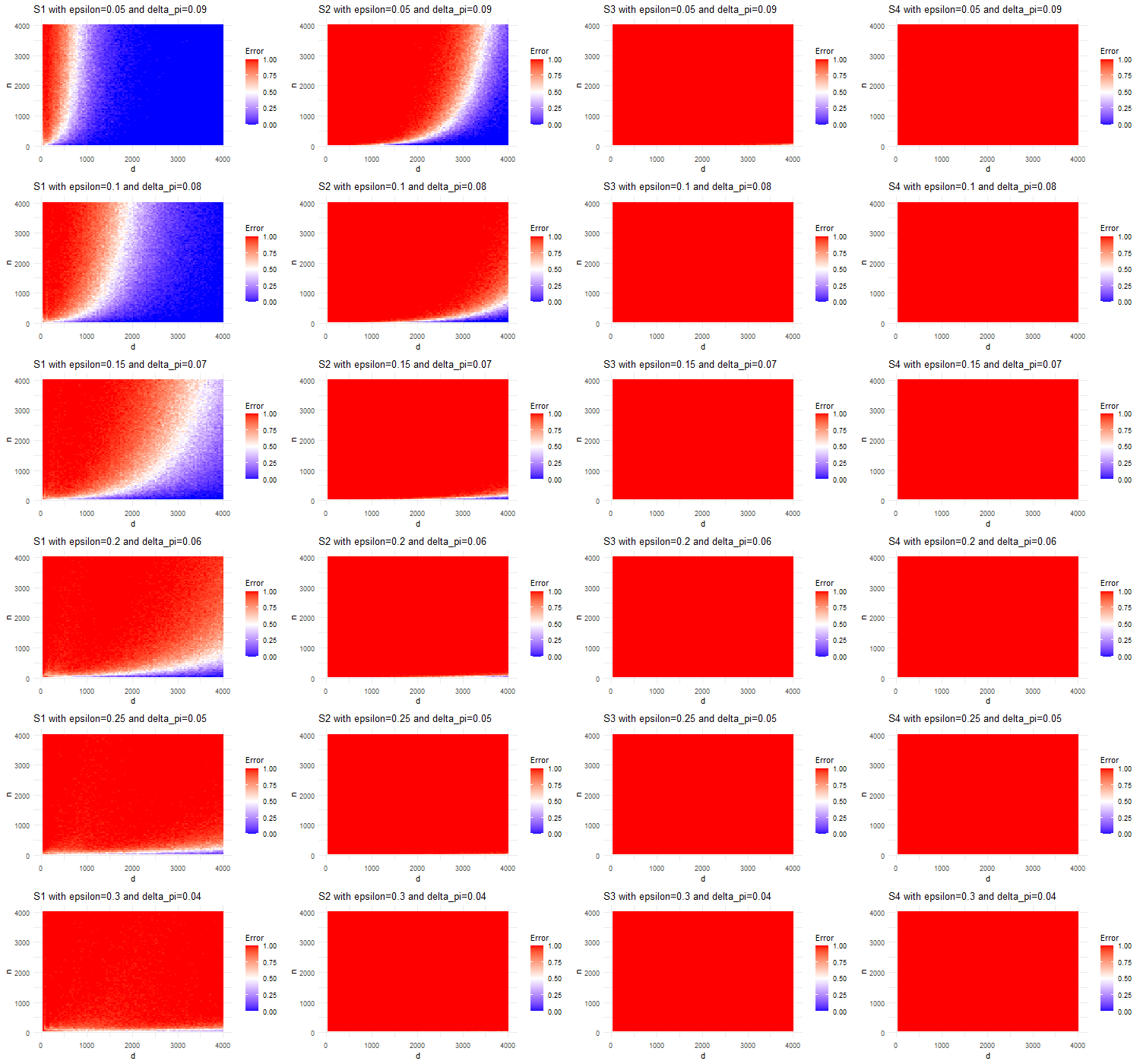
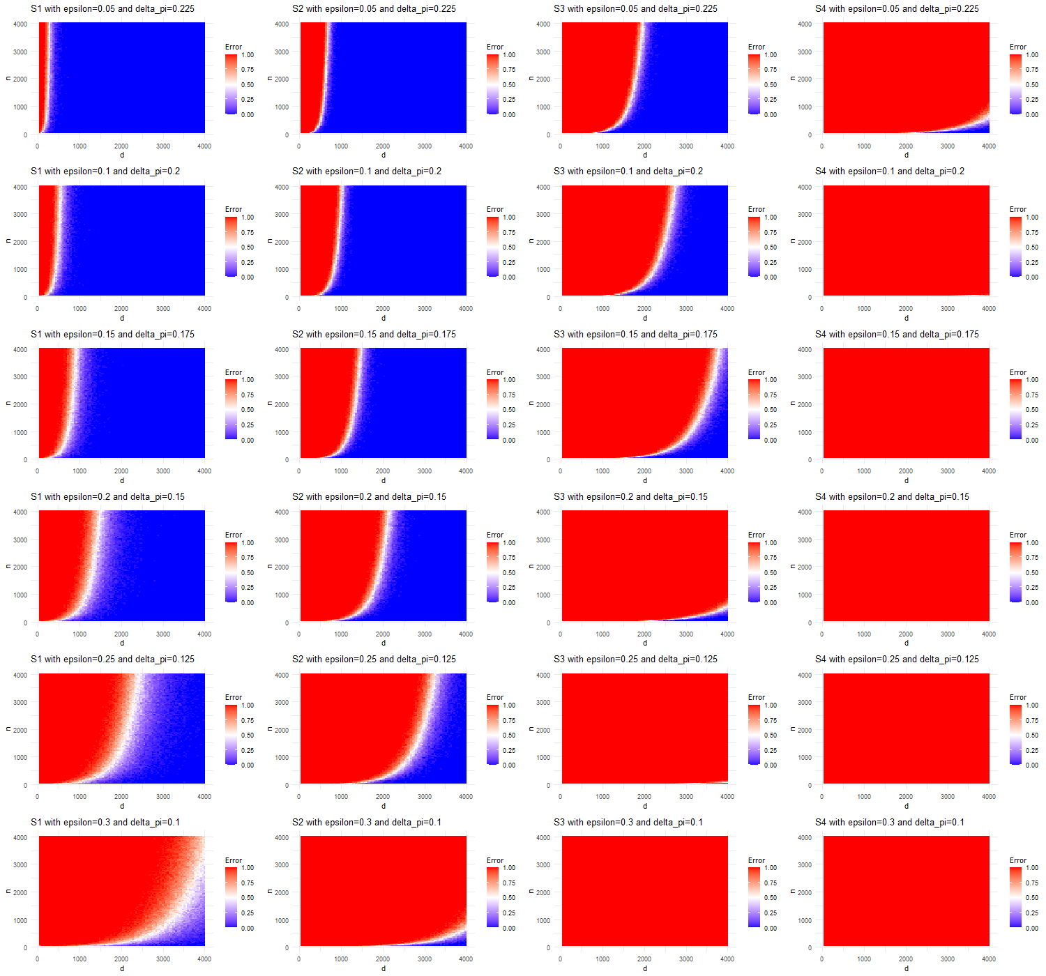
Figures 2 and 3 show the proportions of bad estimations of gsuperscript𝑔g^{\star} following the parameters ε𝜀\varepsilon (in rows) as function of the number of rows n𝑛n, the numbers of columns d𝑑d and the thresholds used (columns). For each figure, the number of columns (d𝑑d) increases on the x-axis and the number of rows (n𝑛n) increases on the x-axis. The red color corresponds to a bad estimate while the blue color corresponds to a good estimate (the more blue it is, the better).
Refer to caption
Figure 2: Proportions of bad estimations of gsuperscript𝑔g^{\star} for the parameter ε{0.05,,0.3}𝜀0.050.3\varepsilon\in\{0.05,\ldots,0.3\} (in rows) following the thresholds (in columns) used for the balanced case: for each graphic, the number of rows n𝑛n (y-axis) and the number of columns d𝑑d (x-axis) varies between 20 and 4000.

As expected, it appears that the best threshold is the oracle S1=δ𝝅/2subscript𝑆1subscript𝛿superscript𝝅2S_{1}=\delta_{\boldsymbol{\pi}^{\star}}/2 but this threshold cannot be used in practice because δ𝝅subscript𝛿superscript𝝅\delta_{\boldsymbol{\pi}^{\star}} is unknown. For the scaled thresholds, S2n,d=2logn/d(1+1010)superscriptsubscript𝑆2𝑛𝑑2𝑛𝑑1superscript1010S_{2}^{n,d}=\sqrt{2\log n/d}\left(1+10^{-10}\right) is the best.

Refer to caption
Figure 3: Proportions of bad estimations of gsuperscript𝑔g^{\star} for the parameter ε{0.05,,0.3}𝜀0.050.3\varepsilon\in\{0.05,\ldots,0.3\} (in rows) following the thresholds (in columns) used for the arithmetic case: for each graphic, the number of rows n𝑛n (y-axis) and the number of columns d𝑑d (x-axis) varies between 20 and 4000.

We can see that the larger the number of rows n𝑛n is, the worse the estimation is and the larger the number of columns d𝑑d is, the better the estimation is. In the case of n=d𝑛𝑑n=d, the quality of the estimation increases with n𝑛n. In particular, the model selection can be generalized for the case of channarond2011Classification and the results would be similar. πminsuperscriptsubscript𝜋\pi_{\min}^{\star} has a weak effect because it is rare to have an empty class but the effect of δ𝝅subscript𝛿superscript𝝅\delta_{\boldsymbol{\pi}^{\star}} seems to be greater.

6.2 Estimation of the parameters

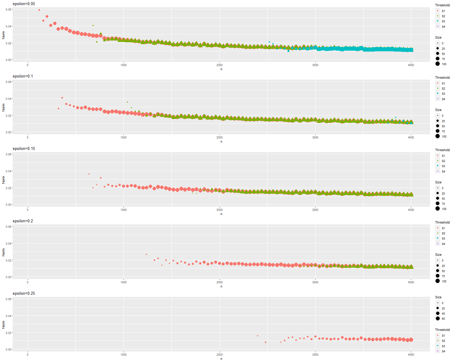
To illustrate the convergence of the the estimation 𝜽^^𝜽\widehat{\boldsymbol{\theta}} to the true parameter 𝜽superscript𝜽\boldsymbol{\theta}^{\star}, the same experimental design is chosen with the number of rows n𝑛n and the number of columns d𝑑d vary between 40 and 4000 by step 40 and, for each configuration, 100 matrices were simulated. To estimate the quality of the estimation, the distance dsuperscript𝑑d^{\infty} introduced in Section 5.1 is calculated. As the distance equals ++\infty when the number of clusters of 𝜽^^𝜽\widehat{\boldsymbol{\theta}} is different of its of 𝜽superscript𝜽\boldsymbol{\theta}^{\star}, we chose to represent the mean of the finite values with the size of the point corresponding at the number of finite values (see Figure 4 for the balanced case and Figure 7 for the arithmetic case).
Refer to caption
Figure 4: Average estimate of the distance d(𝜽,𝜽^)superscript𝑑superscript𝜽^𝜽d^{\infty}\left(\boldsymbol{\theta}^{\star},\widehat{\boldsymbol{\theta}}\right) between the true parameters and the estimated parameters following ε𝜀\varepsilon (rows) in the balanced case: for each graphic, the threshold is represented by different symbols (\bullet for S1subscript𝑆1S_{1}, \blacktriangle for S2n,dsuperscriptsubscript𝑆2𝑛𝑑S_{2}^{n,d}, \blacksquare for S3n,dsuperscriptsubscript𝑆3𝑛𝑑S_{3}^{n,d} and +\boldsymbol{+} for S3n,dsuperscriptsubscript𝑆3𝑛𝑑S_{3}^{n,d}) and the size for the number of finite values used; the number of rows n𝑛n varies between 40 and 4000 and d𝑑d is supposed equal n𝑛n.

We observe that the error decreases with the number of observations and the results are identical when the numbers of clusters are correctly estimated. The optimization of the LG algorithm thus depends on the choice of the threshold. In particular, we find that the oracle threshold (S1subscript𝑆1S_{1}) finds the right number of clusters faster than the evolutionary thresholds. In particular,the threshold S4n,dsuperscriptsubscript𝑆4𝑛𝑑S_{4}^{n,d} does not appear on the graphic because it underestimates the number of blocks.

6.3 Comparison of computing times

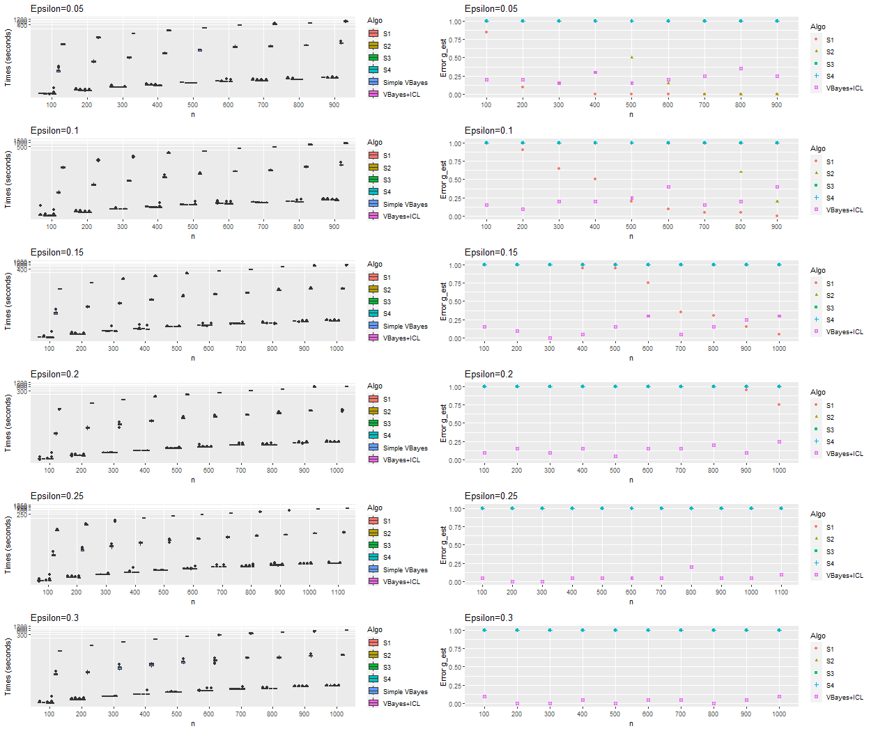
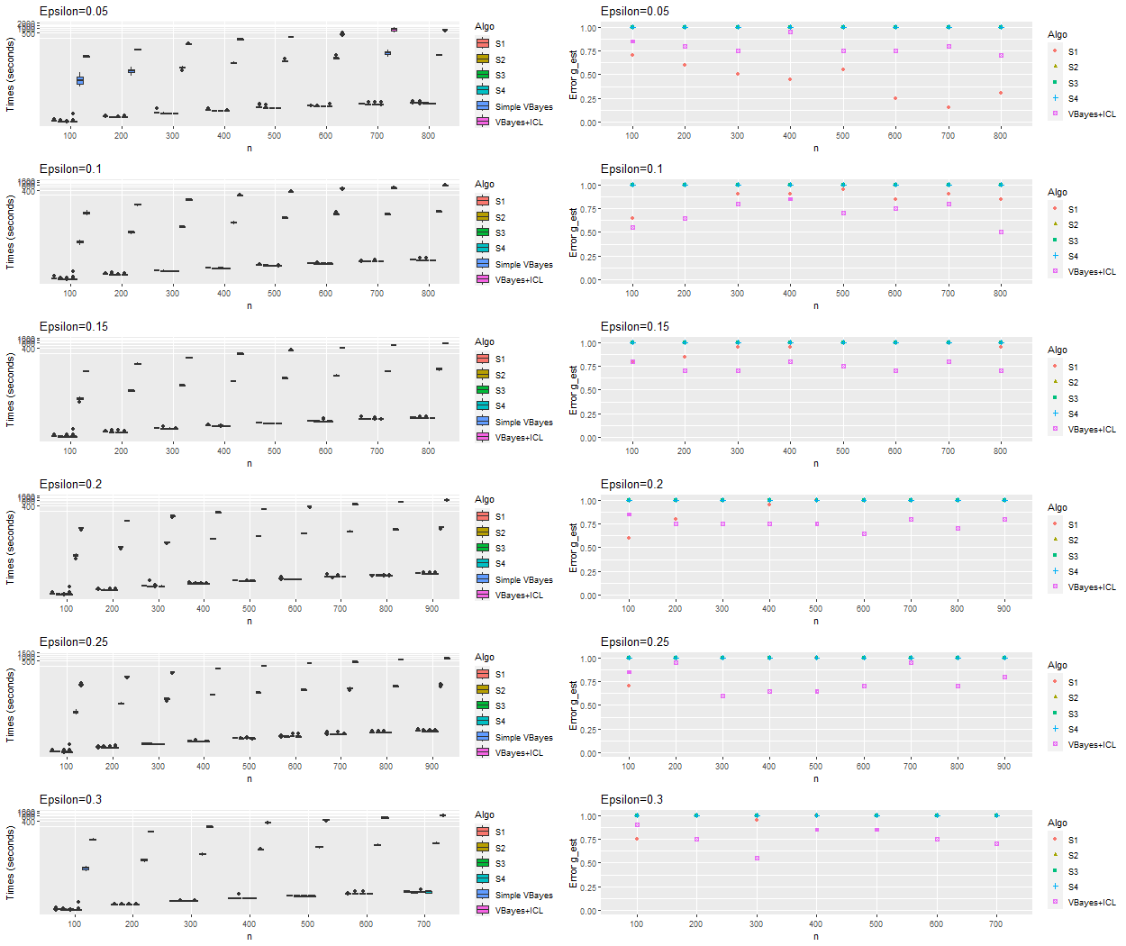
To conclude the part of the simulations, the computation times are estimated and compared with a classical procedure. For that, the plan presented previously is taken again by taking only the square matrices (n=d) with n{100,200,,900}𝑛100200900n\in\{100,200,\ldots,900\} for the balanced case and n{100,200,,700}𝑛100200700n\in\{100,200,\ldots,700\} for the arithmetic. Six procedures are studied:

  • the algorithm LG𝐿𝐺LG with the four previous threshold: S1subscript𝑆1S_{1}, S2n,dsuperscriptsubscript𝑆2𝑛𝑑S_{2}^{n,d}, S3n,dsuperscriptsubscript𝑆3𝑛𝑑S_{3}^{n,d} and S4n,dsuperscriptsubscript𝑆4𝑛𝑑S_{4}^{n,d};

  • the algorithm variational Bayes with the hyperparameters (4,4)44(4,4) as proposed by keribin2014estimation knowing the true number of parameters gsuperscript𝑔g^{\star} and msuperscript𝑚m^{\star} (named Simple VBayes for the next);

  • as the number of blocks is usually unknown, the combination of the algorithm variational Bayes and the Integrated Complete-data Likelihood (see biernacki2000assessing ; keribin2014estimation ) is studied with the hyperparameters (4,4)44(4,4) on a 2×7272\times 7 square grid (named VBayes+ICL for the next).

For the implementation, the R package blockcluster (version 4.5.1; see parmeet2017blockcluster ) with the function coclusterBinary is used. For each configuration, 20 matrices are simulated and procedures are evaluated on two criteria:

  • the mean computation times with 10 runs; for this, the package microbenchmark (version 1.4.9; see olaf2021microbenchmark ) with the function microbenchmark is used and plans are launched on a cluster444Cluster Luke44, 28 cores, 128Go RAM, GPU 2xK40m, 2xIntel Xeon E5-2680 2.40 GHz; more informations on the url https://scalde.gricad-pages.univ-grenoble-alpes.fr/web/pages/presentation.html.

  • the estimation quality of the number of clusters per row after an estimation of each matrix (except for Simple VBayes as the number is assumed be known); results are averaged over the 20 matrices.

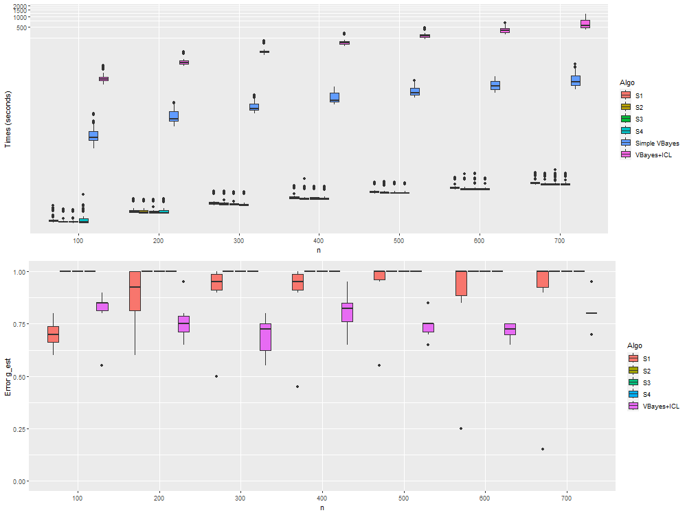
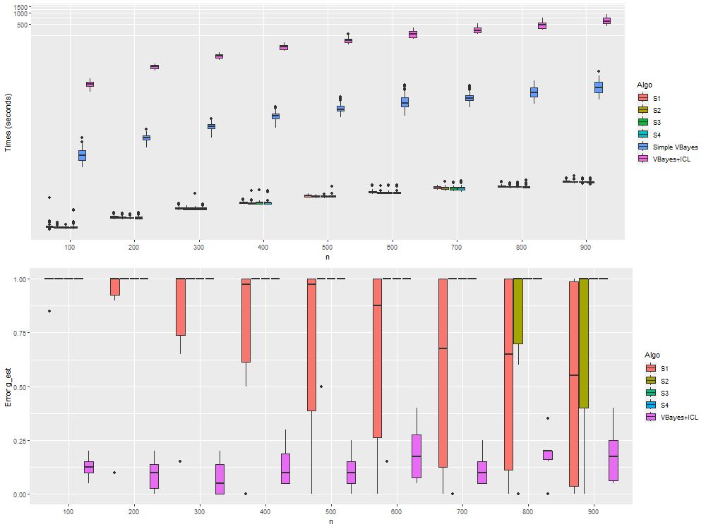
The results are displayed in the Figures 5 (balanced case) and 6 (arithmetic case) where the computation times (in seconds with logarithmic scale; on the top) and the quality of the estimations (averaged for each ε𝜀\varepsilon on over the 20 matrices; on the bottom) have been grouped by matrix size (regardless of the values of ε𝜀\varepsilon). A detailed version for each ε𝜀\varepsilon is available on the Figures 8 and 9 in supplementary material. Moreover, the means and standard deviations (in milliseconds) are represented in the Tables 1 and 2.
Refer to caption
Figure 5: On the top, boxplots of the computing times (in seconds; logarithmic scale) for each procedure (colour) in function of the numbers of rows and columns (n=d𝑛𝑑n=d) over the 1200 simulations (200 per ε𝜀\varepsilon) for the balanced case. On the bottom, boxplots of quality of estimations averaged over the 20 matrices for each ε𝜀\varepsilon for each procedure (colour) in function of the numbers of rows and columns (n=d𝑛𝑑n=d) for the balanced case.
Refer to caption
Figure 6: On the top, boxplots of the computing times (in seconds; logarithmic scale) for each procedure (colour) in function of the numbers of rows and columns (n=d𝑛𝑑n=d) over the 1200 simulations (200 per ε𝜀\varepsilon) for the arithmetic case. On the bottom, boxplots of quality of estimations averaged over the 20 matrices for each ε𝜀\varepsilon for each procedure (colour) in function of the numbers of rows and columns (n=d𝑛𝑑n=d) for the balanced case.
Table 1: Computing times for the different procedures in columns (LG with the four threshold, VBayes with the true number of clusters and VBayes coupled with the ICL criterion on a 2×7272\times 7 square grid) following the number of rows and columns (in rows) for the balanced case. Each cell represents the average (in milliseconds) and the standard deviation (in parenthesis) over the 1200 simulations (200 per ε𝜀\varepsilon).
S1subscript𝑆1S_{1} S2n,dsuperscriptsubscript𝑆2𝑛𝑑S_{2}^{n,d} S3n,dsuperscriptsubscript𝑆3𝑛𝑑S_{3}^{n,d} S4n,dsuperscriptsubscript𝑆4𝑛𝑑S_{4}^{n,d} Simple VBayes VBayes+ICL
n=100 2 2 2 2 171 12765
(0.9) (0.1) (0.1) (0.8) (71.5) (2180.1)
n=200 3 3 3 3 468 37193
(0.4) (0.3) (0.3) (0.3) (102) (4385.4)
n=300 6 6 6 6 930 71594
(0.5) (0.4) (0.9) (0.4) (204.1) (8711.8)
n=400 8 8 8 8 1789 123632
(0.6) (1) (1) (1.4) (461.6) (18941.2)
n=500 13 12 12 12 2934 187319
(0.8) (0.6) (0.6) (1.2) (846.2) (29995)
n=600 16 16 16 16 4597 280348
(1.4) (1) (1.8) (2.1) (2044) (57861.3)
n=700 21 21 21 21 5724 356932
(1.5) (2) (2) (2.6) (1718.6) (61458.8)
n=800 23 22 22 22 8050 490034
(1.6) (1.3) (1.4) (1.9) (2900.3) (107033.6)
n=900 31 30 30 30 11057 629238
(1.9) (2.3) (1.9) (1.8) (4469.8) (136921.4)
Table 2: Computing times for the different procedures in columns (LG with the four threshold, VBayes with the true number of clusters and VBayes coupled with the ICL criterion on a 2×7272\times 7 square grid) following the number of rows and columns (in rows) for the arithmetic case. Each cell represents the average (in milliseconds) and the standard deviation (in parenthesis) over the 120 simulations (20 per ε𝜀\varepsilon).
S1subscript𝑆1S_{1} S2n,dsuperscriptsubscript𝑆2𝑛𝑑S_{2}^{n,d} S3n,dsuperscriptsubscript𝑆3𝑛𝑑S_{3}^{n,d} S4n,dsuperscriptsubscript𝑆4𝑛𝑑S_{4}^{n,d} Simple VBayes VBayes+ICL
n=100 2 2 2 2 530 20819
(0.9) (0.7) (0.7) (1.2) (302.3) (7768.3)
n=200 4 4 4 4 1677 58494
(1.4) (1.4) (1.4) (1.4) (693.7) (18294.9)
n=300 7 7 7 7 3183 117450
(2.4) (2.4) (2.4) (2.4) (1145.8) (34865.2)
n=400 10 10 10 9 5637 203479
(3.2) (3.7) (3.2) (3.3) (2119) (55356.2)
n=500 14 14 13 13 8503 304668
(3.9) (4) (3.9) (3.9) (2862.3) (76486.8)
n=600 18 18 18 18 12423 435626
(5.2) (5.5) (5.9) (5.3) (3889.1) (100281.1)
n=700 25 24 24 24 17794 622631
(6.5) (6.6) (7) (6.8) (7596.6) (180216.9)

On the quality, the procedure VBayes+ICL estimates better than the other the number of clusters in rows and the differences between the four threshold are the same than the section 6.1.

For the computing times, the order of Largest Gaps is that of the millisecond while that of VBayes+ICL is of the second (and the minute after n=300𝑛300n=300). Moreover, the computing time for the Largest Gaps seems to increase linearly with n𝑛n (the side length of the square matrix) as stated in the section 3.2 while VBayes+ICL increases much faster than linearly. Moreover, Largest Gaps does not seem to be impacted by the configuration while the convergence time of VBayes+ICL (and even Simple VBayes who knows the right number of clusters) is larger for the case of arithmetic proportions. And finally, the computation time of VBayes+ICL depends on the maximum choice of the number of clusters (fixed here quite close to the true result) but unknown in practice while Largest Gaps does not need this kind of parameter and the time is almost independent of the number of blocks.

7 Conclusion and discussion

First of all, Largest Gaps is a co-clustering algorithm, which has nice theoretical properties: its computational cost is much lower than most known algorithms and it provides a consistent procedure under the Latent Block Model, for all inference tasks: model selection, classification and estimation of the model parameters. Since the algorithm is simple, the consistency is rather easy to obtain. Note that in this article, only binary matrices have been studied, but the model as well as the method and the proofs can be directly extended for distributions which have the same concentration properties, for example compactly-supported distributions, where the support is known.

As a consistent algorithm, the advantage of the LG algorithm is the simplicity: it is a simple and original way to exploit the concentration of the marginal distributions of the matrix 𝐱𝐱\mathbf{x} under LBM. But it lacks robustness: a single outlier in the marginal distribution can affect the whole classification, which is not desirable by the use on real-world datasets. Moreover, the procedure is essentially based on the choice of threshold and simulations have shown that there is still room for improvement in this choice. Many other algorithms, also based on this nice feature, could be used instead and might be better in practice, but harder to analyze from a theoretical point of view. For example, fitting a binomial mixture model on the variables X(1)¯,X(n)¯¯subscript𝑋1¯subscript𝑋𝑛\overline{X_{(1)\centerdot}},\dots\overline{X_{(n)\centerdot}} with an EM-algorithm, could be fruitful as well.

The contribution of this article actually goes beyond the LG algorithm. It shows special features of the latent structure of the LBM, and their consequences. In particular, when the asymptotic regime of the model is reached, the latent structure is almost obvious, and moreover it can be pick either one but not the two from a summary of the data. Indeed even basic algorithms like LG can retrieve the latent clusters from variables X(1)¯,X(n)¯¯subscript𝑋1¯subscript𝑋𝑛\overline{X_{(1)\centerdot}},\dots\overline{X_{(n)\centerdot}} (sums of the rows and of the columns of the matrix 𝐱𝐱\mathbf{x}), whereas most known classification algorithms are unusable, because of their complexity.

A consequence of this remark is that the LBM should be used sparingly on very large real data sets: if the number of clusters requested is too small and if the blocks are sufficiently contrasted then the marginals should highlight the clusters. If this is not the case, the use of the LBM should be questioned. The bound of the theorem 5.1 would give an estimate of the quality of the use of this model.

Finally, it appears in the simulations that the estimate of the number of clusters is underestimated. Moreover, the distribution of marginals from real-world data rarely has such obvious deviations as assumed by the model asymptotic. To overcome this problem, it would be interesting to estimate the row clusters with a mixture model on the variables (X(1)¯,,X(n)¯)¯subscript𝑋1¯subscript𝑋𝑛(\overline{X_{(1)\centerdot}},\ldots,\overline{X_{(n)\centerdot}}); this will be the subject of future work.

Appendix A Proof of Theorem 5.1

In this appendix, we present demonstrations of the concentration inequality. We first estimate the probability of having the right number of clusters and then the right classification knowing that we have the right number of clusters. Finally, we evaluate the quality of the parameter estimates.

First of all, note that {𝐙^𝒵𝐳}{g^=g}subscript𝒵^𝐙superscript𝐳^𝑔superscript𝑔\{\widehat{\mathbf{Z}}\equiv_{\mathcal{Z}}\mathbf{z}^{\star}\}\subset\{\widehat{g}=g^{\star}\} and {𝐖^𝒲𝐰}{m^=m}subscript𝒲^𝐖superscript𝐰^𝑚superscript𝑚\{\widehat{\mathbf{W}}\equiv_{\mathcal{W}}\mathbf{w}^{\star}\}\subset\{\widehat{m}=m^{\star}\}, hence :

(g^g or m^m or 𝐙^𝒵𝐳 or 𝐖^𝒲𝐰 or d(𝜽^s𝒵,t𝒲,𝜽)>t)^𝑔superscript𝑔 or ^𝑚superscript𝑚 or ^𝐙subscriptnot-equivalent-to𝒵superscript𝐳 or ^𝐖subscriptnot-equivalent-to𝒲superscript𝐰 or superscript𝑑superscript^𝜽subscript𝑠𝒵subscript𝑡𝒲superscript𝜽𝑡\displaystyle\mathbb{P}\left(\widehat{g}\neq g^{\star}\text{ or }\widehat{m}\neq m^{\star}\text{ or }\widehat{\mathbf{Z}}\not\equiv_{\mathcal{Z}}\mathbf{z}^{\star}\text{ or }\widehat{\mathbf{W}}\not\equiv_{\mathcal{W}}\mathbf{w}^{\star}\text{ or }d^{\infty}\left(\widehat{\boldsymbol{\theta}}^{s_{\mathcal{Z}},t_{\mathcal{W}}},\boldsymbol{\theta}^{\star}\right)>t\right)
=\displaystyle= (𝐙^𝒵𝐳 or 𝐖^𝒲𝐰 or d(𝜽^s𝒵,t𝒲,𝜽)>t)subscriptnot-equivalent-to𝒵^𝐙superscript𝐳 or ^𝐖subscriptnot-equivalent-to𝒲superscript𝐰 or superscript𝑑superscript^𝜽subscript𝑠𝒵subscript𝑡𝒲superscript𝜽𝑡\displaystyle\mathbb{P}\left(\widehat{\mathbf{Z}}\not\equiv_{\mathcal{Z}}\mathbf{z}^{\star}\text{ or }\widehat{\mathbf{W}}\not\equiv_{\mathcal{W}}\mathbf{w}^{\star}\text{ or }d^{\infty}\left(\widehat{\boldsymbol{\theta}}^{s_{\mathcal{Z}},t_{\mathcal{W}}},\boldsymbol{\theta}^{\star}\right)>t\right)
=\displaystyle= (𝐙^𝒵𝐳 or 𝐖^𝒲𝐰)+({d(𝜽^s𝒵,t𝒲,𝜽)>t}\{𝐙^𝒵𝐳 or 𝐖^𝒲𝐰})subscriptnot-equivalent-to𝒵^𝐙superscript𝐳 or ^𝐖subscriptnot-equivalent-to𝒲superscript𝐰\superscript𝑑superscript^𝜽subscript𝑠𝒵subscript𝑡𝒲superscript𝜽𝑡subscriptnot-equivalent-to𝒵^𝐙superscript𝐳 or ^𝐖subscriptnot-equivalent-to𝒲superscript𝐰\displaystyle\mathbb{P}\left(\widehat{\mathbf{Z}}\not\equiv_{\mathcal{Z}}\mathbf{z}^{\star}\text{ or }\widehat{\mathbf{W}}\not\equiv_{\mathcal{W}}\mathbf{w}^{\star}\right)+\mathbb{P}\left(\left\{d^{\infty}\left(\widehat{\boldsymbol{\theta}}^{s_{\mathcal{Z}},t_{\mathcal{W}}},\boldsymbol{\theta}^{\star}\right)>t\right\}\left\backslash\left\{\widehat{\mathbf{Z}}\not\equiv_{\mathcal{Z}}\mathbf{z}^{\star}\text{ or }\widehat{\mathbf{W}}\not\equiv_{\mathcal{W}}\mathbf{w}^{\star}\right\}\right.\right)
=\displaystyle= (𝐙^𝒵𝐳 or 𝐖^𝒲𝐰)+(d(𝜽^s𝒵,t𝒲,𝜽)>t,𝐙^𝒵𝐳,𝐖^𝒲𝐰)subscriptnot-equivalent-to𝒵^𝐙superscript𝐳 or ^𝐖subscriptnot-equivalent-to𝒲superscript𝐰formulae-sequencesuperscript𝑑superscript^𝜽subscript𝑠𝒵subscript𝑡𝒲superscript𝜽𝑡formulae-sequencesubscript𝒵^𝐙superscript𝐳subscript𝒲^𝐖superscript𝐰\displaystyle\mathbb{P}\left(\widehat{\mathbf{Z}}\not\equiv_{\mathcal{Z}}\mathbf{z}^{\star}\text{ or }\widehat{\mathbf{W}}\not\equiv_{\mathcal{W}}\mathbf{w}^{\star}\right)+\mathbb{P}\left(d^{\infty}\left(\widehat{\boldsymbol{\theta}}^{s_{\mathcal{Z}},t_{\mathcal{W}}},\boldsymbol{\theta}^{\star}\right)>t,\widehat{\mathbf{Z}}\equiv_{\mathcal{Z}}\mathbf{z}^{\star},\widehat{\mathbf{W}}\equiv_{\mathcal{W}}\mathbf{w}^{\star}\right)
\displaystyle\leq (𝐙^𝒵𝐳)+(𝐖^𝒲𝐰)subscriptnot-equivalent-to𝒵^𝐙superscript𝐳subscriptnot-equivalent-to𝒲^𝐖superscript𝐰\displaystyle\mathbb{P}\left(\widehat{\mathbf{Z}}\not\equiv_{\mathcal{Z}}\mathbf{z}^{\star}\right)+\mathbb{P}\left(\widehat{\mathbf{W}}\not\equiv_{\mathcal{W}}\mathbf{w}^{\star}\right)
+(d(𝜽^s𝒵,t𝒲,𝜽)>t|𝐙^𝒵𝐳,𝐖^𝒲𝐰)(𝐙^𝒵𝐳,𝐖^𝒲𝐰)\displaystyle\quad+\mathbb{P}\left(d^{\infty}\left(\widehat{\boldsymbol{\theta}}^{s_{\mathcal{Z}},t_{\mathcal{W}}},\boldsymbol{\theta}^{\star}\right)>t\left|\widehat{\mathbf{Z}}\equiv_{\mathcal{Z}}\mathbf{z}^{\star},\widehat{\mathbf{W}}\equiv_{\mathcal{W}}\mathbf{w}^{\star}\right.\right)\mathbb{P}\left(\widehat{\mathbf{Z}}\equiv_{\mathcal{Z}}\mathbf{z}^{\star},\widehat{\mathbf{W}}\equiv_{\mathcal{W}}\mathbf{w}^{\star}\right)
\displaystyle\leq (𝐙^𝒵𝐳)+(𝐖^𝒲𝐰)+(d(𝜽^s𝒵,t𝒲,𝜽)>t|𝐙^𝒵𝐳,𝐖^𝒲𝐰)\displaystyle\mathbb{P}\left(\widehat{\mathbf{Z}}\not\equiv_{\mathcal{Z}}\mathbf{z}^{\star}\right)+\mathbb{P}\left(\widehat{\mathbf{W}}\not\equiv_{\mathcal{W}}\mathbf{w}^{\star}\right)+\mathbb{P}\left(d^{\infty}\left(\widehat{\boldsymbol{\theta}}^{s_{\mathcal{Z}},t_{\mathcal{W}}},\boldsymbol{\theta}^{\star}\right)>t\left|\widehat{\mathbf{Z}}\equiv_{\mathcal{Z}}\mathbf{z}^{\star},\widehat{\mathbf{W}}\equiv_{\mathcal{W}}\mathbf{w}^{\star}\right.\right)

To complete the proof, we then need to bound from above the terms of this inequality. The two first terms are bounded using Proposition 1 in Appendix A.1, and the last term is bounded with Proposition 2 in Appendix A.2.

A.1 Concentration inequality on 𝐙^^𝐙\widehat{\mathbf{Z}}

Let us first define the following events.

  • There is at least one individual in each row class, denoted by

    Ag=k=1g{Z+k0}.subscript𝐴superscript𝑔superscriptsubscript𝑘1superscript𝑔subscriptsuperscript𝑍𝑘0A_{g^{\star}}=\bigcap_{k=1}^{g^{\star}}\left\{Z^{\star}_{+k}\neq 0\right\}.
  • Denoting D𝐷D the random variable equal to the maximal distance between Xi¯¯subscript𝑋𝑖\overline{X_{i\centerdot}} and the center of the class of row i𝑖i:

    D=max1kgsupwith zi,k=11in|Xi¯τk|,𝐷1𝑘superscript𝑔1𝑖𝑛with superscriptsubscript𝑧𝑖𝑘1absentsupremum¯subscript𝑋𝑖subscript𝜏𝑘D=\underset{1\leq k\leq g^{\star}}{\max}\;\underset{\overset{1\leq i\leq n}{\underset{\text{with }z_{i,k}^{\star}=1}{}}}{\sup}\;\left|\overline{X_{i\centerdot}}-\tau_{k}\right|,

    we also define:

    ASg={2D<Sg<δ𝝅2D} and Aid=AgASg.subscript𝐴subscript𝑆𝑔2𝐷subscript𝑆𝑔subscript𝛿superscript𝝅2𝐷 and subscript𝐴𝑖𝑑subscript𝐴superscript𝑔subscript𝐴subscript𝑆𝑔A_{S_{g}}=\{2D<S_{g}<\delta_{\boldsymbol{\pi}^{\star}}-2D\}\text{ and }A_{id}=A_{g^{\star}}\cap A_{S_{g}}.
Lemma 1 (Interesting event)
Aid{g^=g}{𝐙^𝒵𝐳}subscript𝐴𝑖𝑑^𝑔superscript𝑔subscript𝒵^𝐙superscript𝐳A_{id}\subset\{\widehat{g}=g^{\star}\}\cap\{\widehat{\mathbf{Z}}\equiv_{\mathcal{Z}}\mathbf{z}^{\star}\}
Proof

On the event ASgsubscript𝐴subscript𝑆𝑔A_{S_{g}}, for any two rows ii{1,,n}𝑖superscript𝑖1𝑛i\neq i^{\prime}\in\{1,\ldots,n\}, we have two possibilities:

  • Either the rows i𝑖i and isuperscript𝑖i^{\prime} are in the same class k𝑘k, and then on ASgsubscript𝐴subscript𝑆𝑔A_{S_{g}}, we have:

    |Xi¯Xi¯||Xi¯τk|+|Xi¯τk|2D<Sg.¯subscript𝑋𝑖¯subscript𝑋superscript𝑖¯subscript𝑋𝑖subscript𝜏𝑘¯subscript𝑋superscript𝑖subscript𝜏𝑘2𝐷subscript𝑆𝑔\left|\overline{X_{i\centerdot}}-\overline{X_{i^{\prime}\centerdot}}\right|\leq\left|\overline{X_{i\centerdot}}-\tau_{k}\right|+\left|\overline{X_{i^{\prime}\centerdot}}-\tau_{k}\right|\leq 2D<S_{g}.\\
  • Or row i𝑖i is in the class k𝑘k and row isuperscript𝑖i^{\prime} in the class kksuperscript𝑘𝑘k^{\prime}\neq k, and on the event ASgsubscript𝐴subscript𝑆𝑔A_{S_{g}}, we have:

    |Xi¯Xi¯|¯subscript𝑋𝑖¯subscript𝑋superscript𝑖\displaystyle\left|\overline{X_{i\centerdot}}-\overline{X_{i^{\prime}\centerdot}}\right| =\displaystyle= |Xi¯τk(Xi¯τk)|¯subscript𝑋𝑖subscript𝜏superscript𝑘¯subscript𝑋superscript𝑖subscript𝜏superscript𝑘\displaystyle\left|\overline{X_{i\centerdot}}-\tau_{k^{\prime}}-\left(\overline{X_{i^{\prime}\centerdot}}-\tau_{k^{\prime}}\right)\right|
    \displaystyle\geq |Xi¯τk||Xi¯τk|¯subscript𝑋𝑖subscript𝜏superscript𝑘¯subscript𝑋superscript𝑖subscript𝜏superscript𝑘\displaystyle\left|\overline{X_{i\centerdot}}-\tau_{k^{\prime}}\right|-\left|\overline{X_{i^{\prime}\centerdot}}-\tau_{k^{\prime}}\right|
    \displaystyle\geq |Xi¯τk|D¯subscript𝑋𝑖subscript𝜏superscript𝑘𝐷\displaystyle\left|\overline{X_{i\centerdot}}-\tau_{k^{\prime}}\right|-D
    \displaystyle\geq |τkτk||Xi¯τk|Dsubscript𝜏𝑘subscript𝜏superscript𝑘¯subscript𝑋𝑖subscript𝜏𝑘𝐷\displaystyle\left|\tau_{k}-\tau_{k^{\prime}}\right|-\left|\overline{X_{i\centerdot}}-\tau_{k}\right|-D
    \displaystyle\geq δ𝝅2Dsubscript𝛿superscript𝝅2𝐷\displaystyle\delta_{\boldsymbol{\pi}^{\star}}-2D
    >\displaystyle> Sg.subscript𝑆𝑔\displaystyle S_{g}.

Therefore, Gi=X(i)¯X(i1)¯subscript𝐺𝑖¯subscript𝑋𝑖¯subscript𝑋𝑖1G_{i}=\overline{X_{(i)\centerdot}}-\overline{X_{(i-1)\centerdot}} is less than Sgsubscript𝑆𝑔S_{g} if and only if both rows (i1)𝑖1(i-1) and (i)𝑖(i) are in the same class. On ASgsubscript𝐴subscript𝑆𝑔A_{S_{g}}, the algorithm hence finds the true classification. Moreover, on Agsubscript𝐴superscript𝑔A_{g^{\star}}, there is at least one row in each class, then the algorithm finds the true number of classes. As a conclusion, on Aidsubscript𝐴𝑖𝑑A_{id}, both g^=g^𝑔superscript𝑔\widehat{g}=g^{\star} and 𝐙^𝒵𝐳subscript𝒵^𝐙superscript𝐳\widehat{\mathbf{Z}}\equiv_{\mathcal{Z}}\mathbf{z}^{\star} are satisfied.

Lemma 2 (Concentration inequality for Aidsubscript𝐴𝑖𝑑A_{id})

Under Assumption (1) and if Sg]0,δ𝛑[ and Sm]0,δ𝛒[S_{g}\in]0,\delta_{\boldsymbol{\pi}^{\star}}[\text{ and }S_{m}\in]0,\delta_{\boldsymbol{\rho}^{\star}}[ for n,d𝑛𝑑n,d large enough:

(Aid¯)2nexp(d2min(δ𝝅Sg,Sg)2)+g(1πmin)n\mathbb{P}\left(\overline{A_{id}}\right)\leq 2n\exp\left(-\frac{d}{2}\min(\delta_{\boldsymbol{\pi}^{\star}}-S_{g},S_{g})^{2}\right)+g^{\star}\left(1-\pi_{\min}^{\star}\right)^{n}

where Aid¯¯subscript𝐴𝑖𝑑\overline{A_{id}} is the complementary of the event Aidsubscript𝐴𝑖𝑑A_{id}.

Proof

Using an union bound, we first obtain:

(Aid¯)(Ag¯)+(ASg¯)¯subscript𝐴𝑖𝑑¯subscript𝐴superscript𝑔¯subscript𝐴subscript𝑆𝑔\mathbb{P}\left(\overline{A_{id}}\right)\leq\mathbb{P}\left(\overline{A_{g^{\star}}}\right)+\mathbb{P}\left(\overline{A_{S_{g}}}\right)

Now we bound from above each of these terms. Again with an union bound:

(Ag¯)¯subscript𝐴superscript𝑔\displaystyle\mathbb{P}\left(\overline{A_{g^{\star}}}\right) =(k=1g{Z+k0}¯)absentsuperscriptsubscript𝑘1superscript𝑔¯subscriptsuperscript𝑍𝑘0\displaystyle=\mathbb{P}\left(\bigcup_{k=1}^{g^{\star}}\overline{\left\{Z^{\star}_{+k}\neq 0\right\}}\right)
k=1g({Z+k0}¯)absentsuperscriptsubscript𝑘1superscript𝑔¯subscriptsuperscript𝑍𝑘0\displaystyle\leq\sum_{k=1}^{g^{\star}}\mathbb{P}\left(\overline{\left\{Z^{\star}_{+k}\neq 0\right\}}\right)
k=1g(Z+k=0)absentsuperscriptsubscript𝑘1superscript𝑔subscriptsuperscript𝑍𝑘0\displaystyle\leq\sum_{k=1}^{g^{\star}}\mathbb{P}\left(Z^{\star}_{+k}=0\right)
k=1gi=1n(Zi,k=0)absentsuperscriptsubscript𝑘1superscript𝑔superscriptsubscriptproduct𝑖1𝑛superscriptsubscript𝑍𝑖𝑘0\displaystyle\leq\sum_{k=1}^{g^{\star}}\prod_{i=1}^{n}\mathbb{P}\left(Z_{i,k}^{\star}=0\right)
k=1gi=1n(1πk)absentsuperscriptsubscript𝑘1superscript𝑔superscriptsubscriptproduct𝑖1𝑛1superscriptsubscript𝜋𝑘\displaystyle\leq\sum_{k=1}^{g^{\star}}\prod_{i=1}^{n}\left(1-\pi_{k}^{\star}\right)
k=1gi=1n(1πmin)absentsuperscriptsubscript𝑘1superscript𝑔superscriptsubscriptproduct𝑖1𝑛1superscriptsubscript𝜋\displaystyle\leq\sum_{k=1}^{g^{\star}}\prod_{i=1}^{n}\left(1-\pi_{\min}^{\star}\right)
g(1πmin)n,absentsuperscript𝑔superscript1superscriptsubscript𝜋𝑛\displaystyle\leq g^{\star}\left(1-\pi_{\min}^{\star}\right)^{n},

which gives the upper bound of the first term. Secondly:

ASgsubscript𝐴subscript𝑆𝑔\displaystyle A_{S_{g}} =\displaystyle= {2D<Sg<δ𝝅2D}2𝐷subscript𝑆𝑔subscript𝛿superscript𝝅2𝐷\displaystyle\{2D<S_{g}<\delta_{\boldsymbol{\pi}^{\star}}-2D\}
=\displaystyle= {2D<Sg,2D<δ𝝅Sg}formulae-sequence2𝐷subscript𝑆𝑔2𝐷subscript𝛿superscript𝝅subscript𝑆𝑔\displaystyle\{2D<S_{g},2D<\delta_{\boldsymbol{\pi}^{\star}}-S_{g}\}
=\displaystyle= {D<12min(δ𝝅Sg,Sg)}.𝐷12subscript𝛿superscript𝝅subscript𝑆𝑔subscript𝑆𝑔\displaystyle\left\{D<\frac{1}{2}\min(\delta_{\boldsymbol{\pi}^{\star}}-S_{g},S_{g})\right\}.

Denoting t=min(δ𝝅Sg,Sg)𝑡subscript𝛿superscript𝝅subscript𝑆𝑔subscript𝑆𝑔t=\min(\delta_{\boldsymbol{\pi}^{\star}}-S_{g},S_{g}),

(ASg¯)¯subscript𝐴subscript𝑆𝑔\displaystyle\mathbb{P}\left(\overline{A_{S_{g}}}\right) =(Dt2)absent𝐷𝑡2\displaystyle=\mathbb{P}\left(D\geq\frac{t}{2}\right)
=(k=1gi|zi,k=1{|Xi¯τk|t2})absentsuperscriptsubscript𝑘1superscript𝑔subscriptconditional𝑖superscriptsubscript𝑧𝑖𝑘1¯subscript𝑋𝑖subscript𝜏𝑘𝑡2\displaystyle=\mathbb{P}\left(\bigcup_{k=1}^{g^{\star}}\bigcup_{i|z_{i,k}^{\star}=1}\left\{\left|\overline{X_{i\centerdot}}-\tau_{k}\right|\geq\frac{t}{2}\right\}\right)
k=1gi|zi,k=1(|Xi¯τk|t2).absentsuperscriptsubscript𝑘1superscript𝑔subscriptconditional𝑖superscriptsubscript𝑧𝑖𝑘1¯subscript𝑋𝑖subscript𝜏𝑘𝑡2\displaystyle\leq\sum_{k=1}^{g^{\star}}\sum_{i|z_{i,k}^{\star}=1}\mathbb{P}\left(\left|\overline{X_{i\centerdot}}-\tau_{k}\right|\geq\frac{t}{2}\right).

Moreover for all i{1,,n}𝑖1𝑛i\in\{1,\ldots,n\}, given zi,k=1superscriptsubscript𝑧𝑖𝑘1z_{i,k}^{\star}=1, Xi+subscript𝑋limit-from𝑖X_{i+} has a binomial distribution in(d,τk)𝑖𝑛𝑑subscript𝜏𝑘\mathcal{B}in\left(d,\tau_{k}\right). The concentration properties of this distribution are then exploited through the Hoeffding inequality:

(|Xi¯τk|t2)=(|Xi+dτk|dt2)¯subscript𝑋𝑖subscript𝜏𝑘𝑡2subscript𝑋limit-from𝑖𝑑subscript𝜏𝑘𝑑𝑡2\displaystyle\mathbb{P}\left(\left|\overline{X_{i\centerdot}}-\tau_{k}\right|\geq\frac{t}{2}\right)=\mathbb{P}\left(\left|X_{i+}-d\tau_{k}\right|\geq\frac{dt}{2}\right) \displaystyle\leq 2e12dt2.2superscript𝑒12𝑑superscript𝑡2\displaystyle 2e^{-\frac{1}{2}dt^{2}}.

And as a conclusion, the bound of the second term is:

(ASg¯)k=1gi|zi,k=12e12dt2=2ne12dt2.¯subscript𝐴subscript𝑆𝑔superscriptsubscript𝑘1superscript𝑔subscriptconditional𝑖superscriptsubscript𝑧𝑖𝑘12superscript𝑒12𝑑superscript𝑡22𝑛superscript𝑒12𝑑superscript𝑡2\mathbb{P}\left(\overline{A_{S_{g}}}\right)\leq\sum_{k=1}^{g^{\star}}\sum_{i|z_{i,k}^{\star}=1}2e^{-\frac{1}{2}dt^{2}}=2ne^{-\frac{1}{2}dt^{2}}.

With these two lemmas, the following proposition is obtained

Proposition 1

Under Assumption (1) and if Sg]0,δ𝛑[ and Sm]0,δ𝛒[S_{g}\in]0,\delta_{\boldsymbol{\pi}^{\star}}[\text{ and }S_{m}\in]0,\delta_{\boldsymbol{\rho}^{\star}}[ for n,d𝑛𝑑n,d large enough:

(𝐙^𝒵𝐳)subscriptnot-equivalent-to𝒵^𝐙superscript𝐳\displaystyle\mathbb{P}\left(\widehat{\mathbf{Z}}\not\equiv_{\mathcal{Z}}\mathbf{z}^{\star}\right) \displaystyle\leq 2nexp(d2min(δ𝝅Sg,Sg)2)+g(1πmin)n.\displaystyle 2n\exp\left(-\frac{d}{2}\min(\delta_{\boldsymbol{\pi}^{\star}}-S_{g},S_{g})^{2}\right)+g^{\star}\left(1-\pi_{\min}^{\star}\right)^{n}.
(𝐖^𝒲𝐰)subscriptnot-equivalent-to𝒲^𝐖superscript𝐰\displaystyle\mathbb{P}\left(\widehat{\mathbf{W}}\not\equiv_{\mathcal{W}}\mathbf{w}^{\star}\right) \displaystyle\leq 2dexp(n2min(δ𝝆Sm,Sm)2)+m(1ρmin)d.\displaystyle 2d\exp\left(-\frac{n}{2}\min(\delta_{\boldsymbol{\rho}^{\star}}-S_{m},S_{m})^{2}\right)+m^{\star}\left(1-\rho_{\min}^{\star}\right)^{d}.
Proof

Lemma 1 tells that whenever the event Aidsubscript𝐴𝑖𝑑A_{id} is satisfied, then both true number of row classes and their true classification are obtained. Lemma 2 provides an upper bound of (Aid¯)¯subscript𝐴𝑖𝑑\mathbb{P}\left(\overline{A_{id}}\right). From these lemmas, it is directly deduced that:

(𝐙^𝒵𝐳)subscriptnot-equivalent-to𝒵^𝐙superscript𝐳\displaystyle\mathbb{P}\left(\widehat{\mathbf{Z}}\not\equiv_{\mathcal{Z}}\mathbf{z}^{\star}\right) \displaystyle\leq (Aid¯)¯subscript𝐴𝑖𝑑\displaystyle\mathbb{P}\left(\overline{A_{id}}\right)
\displaystyle\leq 2nexp(d2min(δ𝝅Sg,Sg)2)+g(1πmin)n,\displaystyle 2n\exp\left(-\frac{d}{2}\min(\delta_{\boldsymbol{\pi}^{\star}}-S_{g},S_{g})^{2}\right)+g^{\star}\left(1-\pi_{\min}^{\star}\right)^{n},

which is Proposition 1.

A.2 Concentration inequality on d(𝜽^s𝒵,t𝒲,𝜽)>tsuperscript𝑑superscript^𝜽subscript𝑠𝒵subscript𝑡𝒲superscript𝜽𝑡d^{\infty}\left(\widehat{\boldsymbol{\theta}}^{s_{\mathcal{Z}},t_{\mathcal{W}}},\boldsymbol{\theta}^{\star}\right)>t

In this part, the proof of the inequality on d(𝜽^s𝒵,t𝒲,𝜽)>tsuperscript𝑑superscript^𝜽subscript𝑠𝒵subscript𝑡𝒲superscript𝜽𝑡d^{\infty}\left(\widehat{\boldsymbol{\theta}}^{s_{\mathcal{Z}},t_{\mathcal{W}}},\boldsymbol{\theta}^{\star}\right)>t is detailled.

Proposition 2

For all t>0𝑡0t>0, we have:

(d(𝜽^s𝒵,t𝒲,𝜽)>t|𝐙^𝒵𝐳,𝐖^𝒲𝐰)\displaystyle\!\!\!\!\!\!\!\!\!\!\!\!\mathbb{P}\left(d^{\infty}\left(\widehat{\boldsymbol{\theta}}^{s_{\mathcal{Z}},t_{\mathcal{W}}},\boldsymbol{\theta}^{\star}\right)>t\left|\widehat{\mathbf{Z}}\equiv_{\mathcal{Z}}\mathbf{z}^{\star},\widehat{\mathbf{W}}\equiv_{\mathcal{W}}\mathbf{w}^{\star}\right.\right)
\displaystyle\leq 2gm[1πminρmin(1e2t2)]nd+2ge2nt2+2me2dt22superscript𝑔superscript𝑚superscriptdelimited-[]1superscriptsubscript𝜋superscriptsubscript𝜌1superscript𝑒2superscript𝑡2𝑛𝑑2superscript𝑔superscript𝑒2𝑛superscript𝑡22superscript𝑚superscript𝑒2𝑑superscript𝑡2\displaystyle 2g^{\star}m^{\star}\left[1-\pi_{\min}^{\star}\rho_{\min}^{\star}\left(1-e^{-2t^{2}}\right)\right]^{nd}+2g^{\star}e^{-2nt^{2}}+2m^{\star}e^{-2dt^{2}}

The proof consists in obtaining three bounds: one for each parameter. The inequalities on 𝝅𝝅\boldsymbol{\pi} and 𝝆𝝆\boldsymbol{\rho} are an application of the Hoeffding inequality and are similar to channarond2011Classification for the row class proportions. To obtain the inequality for 𝜶𝜶\boldsymbol{\alpha}, it is necessary to study the conditional probability, given the true partition (𝐳,𝐰)superscript𝐳superscript𝐰\left(\mathbf{z}^{\star},\mathbf{w}^{\star}\right). Apart from the problem of two asymptotic behaviors, the proof is similar to channarond2011Classification .

In the sequel, and for ease of reading, we remove the superscripts s𝒵subscript𝑠𝒵s_{\mathcal{Z}} and t𝒲subscript𝑡𝒲t_{\mathcal{W}}. Therefore, for all t>0𝑡0t>0:

(d(𝜽^,𝜽)>t|𝐙^𝒵𝐳,𝐖^𝒲𝐰)\displaystyle\!\!\!\!\!\!\!\!\!\!\!\!\mathbb{P}\left(d^{\infty}\left(\widehat{\boldsymbol{\theta}},\boldsymbol{\theta}^{\star}\right)>t\left|\widehat{\mathbf{Z}}\equiv_{\mathcal{Z}}\mathbf{z}^{\star},\widehat{\mathbf{W}}\equiv_{\mathcal{W}}\mathbf{w}^{\star}\right.\right)
=\displaystyle= (max(𝝅^𝝅,𝝆^𝝆,𝜶^𝜶)>t|𝐙^𝒵𝐳,𝐖^𝒲𝐰)\displaystyle\mathbb{P}\left(\max\left(\left\|\widehat{\boldsymbol{\pi}}-\boldsymbol{\pi}^{\star}\right\|_{\infty},\left\|\widehat{\boldsymbol{\rho}}-\boldsymbol{\rho}^{\star}\right\|_{\infty},\left\|\widehat{\boldsymbol{\alpha}}-\boldsymbol{\alpha}^{\star}\right\|_{\infty}\right)>t\left|\widehat{\mathbf{Z}}\equiv_{\mathcal{Z}}\mathbf{z}^{\star},\widehat{\mathbf{W}}\equiv_{\mathcal{W}}\mathbf{w}^{\star}\right.\right)
\displaystyle\leq (𝝅^𝝅>t|𝐙^𝒵𝐳,𝐖^𝒲𝐰)+(𝝆^𝝆>t|𝐙^𝒵𝐳,𝐖^𝒲𝐰)\displaystyle\mathbb{P}\left(\left\|\widehat{\boldsymbol{\pi}}-\boldsymbol{\pi}^{\star}\right\|_{\infty}>t\left|\widehat{\mathbf{Z}}\equiv_{\mathcal{Z}}\mathbf{z}^{\star},\widehat{\mathbf{W}}\equiv_{\mathcal{W}}\mathbf{w}^{\star}\right.\right)+\mathbb{P}\left(\left\|\widehat{\boldsymbol{\rho}}-\boldsymbol{\rho}^{\star}\right\|_{\infty}>t\left|\widehat{\mathbf{Z}}\equiv_{\mathcal{Z}}\mathbf{z}^{\star},\widehat{\mathbf{W}}\equiv_{\mathcal{W}}\mathbf{w}^{\star}\right.\right)
+(𝜶^𝜶>t|𝐙^𝒵𝐳,𝐖^𝒲𝐰)\displaystyle+\mathbb{P}\left(\left\|\widehat{\boldsymbol{\alpha}}-\boldsymbol{\alpha}^{\star}\right\|_{\infty}>t\left|\widehat{\mathbf{Z}}\equiv_{\mathcal{Z}}\mathbf{z}^{\star},\widehat{\mathbf{W}}\equiv_{\mathcal{W}}\mathbf{w}^{\star}\right.\right)
\displaystyle\leq k=1g(|πk^πk|>t|𝐙^𝒵𝐳,𝐖^𝒲𝐰)+=1m(|ρ^ρ|>t|𝐙^𝒵𝐳,𝐖^𝒲𝐰)\displaystyle\sum_{k=1}^{g^{\star}}\mathbb{P}\left(\left|\widehat{\pi_{k}}-\pi_{k}^{\star}\right|>t\left|\widehat{\mathbf{Z}}\equiv_{\mathcal{Z}}\mathbf{z}^{\star},\widehat{\mathbf{W}}\equiv_{\mathcal{W}}\mathbf{w}^{\star}\right.\right)+\sum_{\ell=1}^{m^{\star}}\mathbb{P}\left(\left|\widehat{\rho_{\ell}}-\rho_{\ell}^{\star}\right|>t\left|\widehat{\mathbf{Z}}\equiv_{\mathcal{Z}}\mathbf{z}^{\star},\widehat{\mathbf{W}}\equiv_{\mathcal{W}}\mathbf{w}^{\star}\right.\right)
+k=1g=1m(|αk^αk|>t|𝐙^𝒵𝐳,𝐖^𝒲𝐰).\displaystyle+\sum_{k=1}^{g^{\star}}\sum_{\ell=1}^{m^{\star}}\mathbb{P}\left(\left|\widehat{\alpha_{k\ell}}-\alpha_{k\ell}^{\star}\right|>t\left|\widehat{\mathbf{Z}}\equiv_{\mathcal{Z}}\mathbf{z}^{\star},\widehat{\mathbf{W}}\equiv_{\mathcal{W}}\mathbf{w}^{\star}\right.\right).

The upper bounds of the first and second terms are the same as channarond2011Classification ; only the last term is different. For αk^^subscript𝛼𝑘\widehat{\alpha_{k\ell}}, first note that when 𝐙^𝒵𝐳subscript𝒵^𝐙superscript𝐳\widehat{\mathbf{Z}}\equiv_{\mathcal{Z}}\mathbf{z}^{\star} and 𝐖^𝒲𝐰subscript𝒲^𝐖superscript𝐰\widehat{\mathbf{W}}\equiv_{\mathcal{W}}\mathbf{w}^{\star}

αk^=αk~=1z+kw+(i,j)|zi,kwj,=1Xij^subscript𝛼𝑘~subscript𝛼𝑘1subscriptsuperscript𝑧𝑘subscriptsuperscript𝑤subscriptconditional𝑖𝑗superscriptsubscript𝑧𝑖𝑘superscriptsubscript𝑤𝑗1subscript𝑋𝑖𝑗\widehat{\alpha_{k\ell}}=\widetilde{\alpha_{k\ell}}=\frac{1}{z^{\star}_{+k}w^{\star}_{+\ell}}\sum_{\left(i,j\right)\left|z_{i,k}^{\star}w_{j,\ell}^{\star}=1\right.}X_{ij}

and given (𝐳,𝐰)superscript𝐳superscript𝐰\left(\mathbf{z}^{\star},\mathbf{w}^{\star}\right), the Hoeffding inequality gives for all t>0𝑡0t>0:

(|αk^αk|>t|𝐙^𝒵𝐳,𝐖^𝒲𝐰)\displaystyle\mathbb{P}\left(\left|\widehat{\alpha_{k\ell}}-\alpha_{k\ell}^{\star}\right|>t\left|\widehat{\mathbf{Z}}\equiv_{\mathcal{Z}}\mathbf{z}^{\star},\widehat{\mathbf{W}}\equiv_{\mathcal{W}}\mathbf{w}^{\star}\right.\right) =\displaystyle= (|αk~αk|>t|𝐙^𝒵𝐳,𝐖^𝒲𝐰)\displaystyle\mathbb{P}\left(\left|\widetilde{\alpha_{k\ell}}-\alpha^{\star}_{k\ell}\right|>t\left|\widehat{\mathbf{Z}}\equiv_{\mathcal{Z}}\mathbf{z}^{\star},\widehat{\mathbf{W}}\equiv_{\mathcal{W}}\mathbf{w}^{\star}\right.\right)
\displaystyle\leq (|αk~αk|>t)~subscript𝛼𝑘subscriptsuperscript𝛼𝑘𝑡\displaystyle\mathbb{P}\left(\left|\widetilde{\alpha_{k\ell}}-\alpha^{\star}_{k\ell}\right|>t\right)
\displaystyle\leq 𝔼𝐙,𝐖[(|αk~αk|>t|𝐙,𝐖)]subscript𝔼superscript𝐙superscript𝐖delimited-[]~subscript𝛼𝑘subscriptsuperscript𝛼𝑘conditional𝑡superscript𝐙superscript𝐖\displaystyle\mathbb{E}_{\mathbf{Z}^{\star},\mathbf{W}^{\star}}\left[\left.\mathbb{P}\left(\left|\widetilde{\alpha_{k\ell}}-\alpha^{\star}_{k\ell}\right|>t\right|\mathbf{Z}^{\star},\mathbf{W}^{\star}\right)\right]
\displaystyle\leq 𝔼𝐙,𝐖[2e2Z+kW+t2].subscript𝔼superscript𝐙superscript𝐖delimited-[]2superscript𝑒2subscriptsuperscript𝑍𝑘subscriptsuperscript𝑊superscript𝑡2\displaystyle\mathbb{E}_{\mathbf{Z}^{\star},\mathbf{W}^{\star}}\left[2e^{-2Z^{\star}_{+k}W^{\star}_{+\ell}t^{2}}\right].

But, as z+k=i=1nzi,ksubscriptsuperscript𝑧𝑘superscriptsubscript𝑖1𝑛superscriptsubscript𝑧𝑖𝑘z^{\star}_{+k}=\sum_{i=1}^{n}z_{i,k}^{\star} and w+=j=1dwj,subscriptsuperscript𝑤superscriptsubscript𝑗1𝑑superscriptsubscript𝑤𝑗w^{\star}_{+\ell}=\sum_{j=1}^{d}w_{j,\ell}^{\star} and the variables are independents, the expectation is:

𝔼𝐙,𝐖[2e2Z+kW+t2]subscript𝔼superscript𝐙superscript𝐖delimited-[]2superscript𝑒2subscriptsuperscript𝑍𝑘subscriptsuperscript𝑊superscript𝑡2\displaystyle\mathbb{E}_{\mathbf{Z}^{\star},\mathbf{W}^{\star}}\left[2e^{-2Z^{\star}_{+k}W^{\star}_{+\ell}t^{2}}\right] =\displaystyle= 2𝔼𝐙,𝐖[exp(2i=1nZi,kj=1dWjt2)]2subscript𝔼superscript𝐙superscript𝐖delimited-[]2superscriptsubscript𝑖1𝑛superscriptsubscript𝑍𝑖𝑘superscriptsubscript𝑗1𝑑superscriptsubscript𝑊𝑗superscript𝑡2\displaystyle 2\mathbb{E}_{\mathbf{Z}^{\star},\mathbf{W}^{\star}}\left[\exp\left(-2\sum_{i=1}^{n}Z_{i,k}^{\star}\sum_{j=1}^{d}W_{j\ell}^{\star}t^{2}\right)\right]
=\displaystyle= 𝔼𝐙,𝐖[2i=1nexp(2Zi,kj=1dWjt2)]subscript𝔼superscript𝐙superscript𝐖delimited-[]2superscriptsubscriptproduct𝑖1𝑛2superscriptsubscript𝑍𝑖𝑘superscriptsubscript𝑗1𝑑superscriptsubscript𝑊𝑗superscript𝑡2\displaystyle\mathbb{E}_{\mathbf{Z}^{\star},\mathbf{W}^{\star}}\left[2\prod_{i=1}^{n}\exp\left(-2Z_{i,k}^{\star}\sum_{j=1}^{d}W_{j\ell}^{\star}t^{2}\right)\right]
=\displaystyle= 2i=1n𝔼𝐙,𝐖[exp(2Zi,kj=1dWjt2)]2superscriptsubscriptproduct𝑖1𝑛subscript𝔼superscript𝐙superscript𝐖delimited-[]2superscriptsubscript𝑍𝑖𝑘superscriptsubscript𝑗1𝑑superscriptsubscript𝑊𝑗superscript𝑡2\displaystyle 2\prod_{i=1}^{n}\mathbb{E}_{\mathbf{Z}^{\star},\mathbf{W}^{\star}}\left[\exp\left(-2Z_{i,k}^{\star}\sum_{j=1}^{d}W_{j\ell}^{\star}t^{2}\right)\right]
=\displaystyle= 2i=1nj=1d𝔼𝐙,𝐖[exp(2Zi,kWjt2)]2superscriptsubscriptproduct𝑖1𝑛superscriptsubscriptproduct𝑗1𝑑subscript𝔼superscript𝐙superscript𝐖delimited-[]2superscriptsubscript𝑍𝑖𝑘superscriptsubscript𝑊𝑗superscript𝑡2\displaystyle 2\prod_{i=1}^{n}\prod_{j=1}^{d}\mathbb{E}_{\mathbf{Z}^{\star},\mathbf{W}^{\star}}\left[\exp\left(-2Z_{i,k}^{\star}W_{j\ell}^{\star}t^{2}\right)\right]

Since, for all i{1,,n}𝑖1𝑛i\in\{1,\ldots,n\}, j{1,,d}𝑗1𝑑j\in\{1,\ldots,d\}, k{1,,g}𝑘1superscript𝑔k\in\{1,\ldots,g^{\star}\} and {1,,m}1superscript𝑚\ell\in\{1,\ldots,m^{\star}\}, the variable Zi,kWjsuperscriptsubscript𝑍𝑖𝑘superscriptsubscript𝑊𝑗Z_{i,k}^{\star}W_{j\ell}^{\star} is a Bernoulli of parameter πkρsuperscriptsubscript𝜋𝑘superscriptsubscript𝜌\pi_{k}^{\star}\rho_{\ell}^{\star}, then:

𝔼𝐙,𝐖[exp(2zi,kwj,t2)]subscript𝔼superscript𝐙superscript𝐖delimited-[]2superscriptsubscript𝑧𝑖𝑘superscriptsubscript𝑤𝑗superscript𝑡2\displaystyle\mathbb{E}_{\mathbf{Z}^{\star},\mathbf{W}^{\star}}\left[\exp\left(-2z_{i,k}^{\star}w_{j,\ell}^{\star}t^{2}\right)\right] =\displaystyle= πkρexp(2×1×t2)+(1πkρ)exp(2×0×t2)superscriptsubscript𝜋𝑘superscriptsubscript𝜌21superscript𝑡21superscriptsubscript𝜋𝑘superscriptsubscript𝜌20superscript𝑡2\displaystyle\pi_{k}^{\star}\rho_{\ell}^{\star}\exp\left(-2\times 1\times t^{2}\right)+\left(1-\pi_{k}^{\star}\rho_{\ell}^{\star}\right)\exp\left(-2\times 0\times t^{2}\right)
=\displaystyle= πkρexp(2t2)+1πkρsuperscriptsubscript𝜋𝑘superscriptsubscript𝜌2superscript𝑡21superscriptsubscript𝜋𝑘superscriptsubscript𝜌\displaystyle\pi_{k}^{\star}\rho_{\ell}^{\star}\exp\left(-2t^{2}\right)+1-\pi_{k}^{\star}\rho_{\ell}^{\star}
=\displaystyle= 1πkρ(1e2t2).1superscriptsubscript𝜋𝑘superscriptsubscript𝜌1superscript𝑒2superscript𝑡2\displaystyle 1-\pi_{k}^{\star}\rho_{\ell}^{\star}\left(1-e^{-2t^{2}}\right).

Finally, the inequality is:

(|αk^αk|>t|𝐙^𝒵𝐳,𝐖^𝒲𝐰)\displaystyle\mathbb{P}\left(\left|\widehat{\alpha_{k\ell}}-\alpha_{k\ell}^{\star}\right|>t\left|\widehat{\mathbf{Z}}\equiv_{\mathcal{Z}}\mathbf{z}^{\star},\widehat{\mathbf{W}}\equiv_{\mathcal{W}}\mathbf{w}^{\star}\right.\right) \displaystyle\leq [1πkρ(1e2t2)]ndsuperscriptdelimited-[]1superscriptsubscript𝜋𝑘superscriptsubscript𝜌1superscript𝑒2superscript𝑡2𝑛𝑑\displaystyle\left[1-\pi_{k}^{\star}\rho_{\ell}^{\star}\left(1-e^{-2t^{2}}\right)\right]^{nd}
\displaystyle\leq [1πminρmin(1e2t2)]ndsuperscriptdelimited-[]1superscriptsubscript𝜋superscriptsubscript𝜌1superscript𝑒2superscript𝑡2𝑛𝑑\displaystyle\left[1-\pi_{\min}^{\star}\rho_{\min}^{\star}\left(1-e^{-2t^{2}}\right)\right]^{nd}

and the result is obtained by the sum on each cluster.

Appendix B Proof of Theorem 5.2: consistency

The proof is based on Theorem 5.1, as n+𝑛n\to+\infty and d+𝑑d\to+\infty and by the assumption (1), the following limits are obtained for every t>0𝑡0t>0:

g(1πmin)n+m(1ρmin)dsuperscript𝑔superscript1superscriptsubscript𝜋𝑛superscript𝑚superscript1superscriptsubscript𝜌𝑑\displaystyle g^{\star}\left(1-\pi_{\min}^{\star}\right)^{n}+m^{\star}\left(1-\rho_{\min}^{\star}\right)^{d} n,d+𝑛𝑑\displaystyle\underset{n,d\to+\infty}{\longrightarrow} 00\displaystyle 0
and ge2nt2+me2dt2and superscript𝑔superscript𝑒2𝑛superscript𝑡2superscript𝑚superscript𝑒2𝑑superscript𝑡2\displaystyle\text{and }\quad g^{\star}e^{-2nt^{2}}+m^{\star}e^{-2dt^{2}} n,d+𝑛𝑑\displaystyle\underset{n,d\to+\infty}{\longrightarrow} 0.0\displaystyle 0.

For the same reasons, as soon as t𝑡t is positive, 0<πminρmin(1e2t2)<10superscriptsubscript𝜋superscriptsubscript𝜌1superscript𝑒2superscript𝑡210<\pi_{\min}^{\star}\rho_{\min}^{\star}\left(1-e^{-2t^{2}}\right)<1 and

gm[1πminρmin(1e2t2)]ndsuperscript𝑔superscript𝑚superscriptdelimited-[]1superscriptsubscript𝜋superscriptsubscript𝜌1superscript𝑒2superscript𝑡2𝑛𝑑\displaystyle g^{\star}m^{\star}\left[1-\pi_{\min}^{\star}\rho_{\min}^{\star}\left(1-e^{-2t^{2}}\right)\right]^{nd} n,d+𝑛𝑑\displaystyle\underset{n,d\to+\infty}{\longrightarrow} 0.0\displaystyle 0.

For the last terms, the assumption (5.2) gives that

nlog(d)n,d++𝑛𝑑𝑛𝑑\displaystyle\frac{n}{\log(d)}\underset{n,d\to+\infty}{\longrightarrow}+\infty and dlog(n)n,d++𝑑𝑛𝑛𝑑\displaystyle\frac{d}{\log(n)}\underset{n,d\to+\infty}{\longrightarrow}+\infty

which results in

ne12dδ𝝅2+de12nδ𝝆2𝑛superscript𝑒12𝑑superscriptsubscript𝛿superscript𝝅2𝑑superscript𝑒12𝑛superscriptsubscript𝛿superscript𝝆2\displaystyle ne^{-\frac{1}{2}d\delta_{\boldsymbol{\pi}^{\star}}^{2}}+de^{-\frac{1}{2}n\delta_{\boldsymbol{\rho}^{\star}}^{2}} n,d+𝑛𝑑\displaystyle\underset{n,d\to+\infty}{\longrightarrow} 00\displaystyle 0

and, as Sgn,dsuperscriptsubscript𝑆𝑔𝑛𝑑S_{g}^{n,d} tends to zero,

ned(δ𝝅Sgn,d)22n,d+0.𝑛superscript𝑒𝑑superscriptsubscript𝛿superscript𝝅superscriptsubscript𝑆𝑔𝑛𝑑22𝑛𝑑0ne^{-d\frac{\left(\delta_{\boldsymbol{\pi}^{\star}}-S_{g}^{n,d}\right)^{2}}{2}}\underset{n,d\to+\infty}{\longrightarrow}0.

Thanks the same Assumption (5.2), there exists a positive constant C>2𝐶2C>\sqrt{2} such that for n𝑛n and d𝑑d large enough

Sgn,ddlogn>CSgn,d2dlogn>C2>1superscriptsubscript𝑆𝑔𝑛𝑑𝑑𝑛𝐶superscriptsubscript𝑆𝑔𝑛𝑑2𝑑𝑛𝐶21S_{g}^{n,d}\sqrt{\frac{d}{\log n}}>C\Longrightarrow\frac{S_{g}^{n,d}}{\sqrt{2}}\sqrt{\frac{d}{\log n}}>\frac{C}{\sqrt{2}}>1
nedSgn,d22𝑛superscript𝑒𝑑superscriptsuperscriptsubscript𝑆𝑔𝑛𝑑22\displaystyle ne^{-d\frac{{S_{g}^{n,d}}^{2}}{2}} =\displaystyle= exp[logndSgn,d22]𝑛𝑑superscriptsuperscriptsubscript𝑆𝑔𝑛𝑑22\displaystyle\exp\left[\log n-d\frac{{S_{g}^{n,d}}^{2}}{2}\right]
=\displaystyle= exp[logn(1(dlognSgn,d2)2)]𝑛1superscript𝑑𝑛superscriptsubscript𝑆𝑔𝑛𝑑22\displaystyle\exp\left[\log n\left(1-\left(\sqrt{\frac{d}{\log n}}\frac{S_{g}^{n,d}}{\sqrt{2}}\right)^{2}\right)\right]
\displaystyle\leq exp[logn(1C2)<0]𝑛subscript1𝐶2absent0\displaystyle\exp\left[\log n\underbrace{\left(1-\frac{C}{\sqrt{2}}\right)}_{<0}\right]
n,d+𝑛𝑑\displaystyle\underset{n,d\to+\infty}{\longrightarrow} 0.0\displaystyle 0.

Appendix C Proof of Theorem 5.3: consistency in the sparse case

First, if πminn,dsuperscriptsubscript𝜋absent𝑛𝑑\pi_{\min}^{\star\,n,d} tends to zero (and as gn,d1/πminn,dsuperscriptsuperscript𝑔𝑛𝑑1superscriptsubscript𝜋absent𝑛𝑑{g^{\star}}^{n,d}\leq 1/\pi_{\min}^{\star\,n,d}), the series expansion of tlog(1t)maps-to𝑡1𝑡t\mapsto\log(1-t) is used

gn,d(1πminn,d)nsuperscriptsuperscript𝑔𝑛𝑑superscript1superscriptsubscript𝜋absent𝑛𝑑𝑛\displaystyle{g^{\star}}^{n,d}\left(1-\pi_{\min}^{\star\,n,d}\right)^{n} =\displaystyle= exp[loggn,d+nlog(1πminn,d)]superscriptsuperscript𝑔𝑛𝑑𝑛1superscriptsubscript𝜋absent𝑛𝑑\displaystyle\exp\left[\log{g^{\star}}^{n,d}+n\log\left(1-\pi_{\min}^{\star\,n,d}\right)\right]
\displaystyle\leq exp{n[1nlog(1πminn,d)+log(1πminn,d)]}𝑛delimited-[]1𝑛1superscriptsubscript𝜋absent𝑛𝑑1superscriptsubscript𝜋absent𝑛𝑑\displaystyle\exp\left\{n\left[\frac{1}{n}\log\left(\frac{1}{\pi_{\min}^{\star\,n,d}}\right)+\log\left(1-\pi_{\min}^{\star\,n,d}\right)\right]\right\}
\displaystyle\leq exp{n[1nlog(πminn,d)πminn,d+o(πminn,d)]}𝑛delimited-[]1𝑛superscriptsubscript𝜋absent𝑛𝑑superscriptsubscript𝜋absent𝑛𝑑𝑜superscriptsubscript𝜋absent𝑛𝑑\displaystyle\exp\left\{n\left[-\frac{1}{n}\log\left(\pi_{\min}^{\star\,n,d}\right)-\pi_{\min}^{\star\,n,d}+o\left(\pi_{\min}^{\star\,n,d}\right)\right]\right\}
\displaystyle\leq exp{n[πminn,d+o(πminn,d)]}𝑛delimited-[]superscriptsubscript𝜋absent𝑛𝑑𝑜superscriptsubscript𝜋absent𝑛𝑑\displaystyle\exp\left\{n\left[-\pi_{\min}^{\star\,n,d}+o\left(\pi_{\min}^{\star\,n,d}\right)\right]\right\}
\displaystyle\leq exp[nπminn,d+o(nπminn,d)]𝑛superscriptsubscript𝜋absent𝑛𝑑𝑜𝑛superscriptsubscript𝜋absent𝑛𝑑\displaystyle\exp\left[-n\pi_{\min}^{\star\,n,d}+o\left(n\pi_{\min}^{\star\,n,d}\right)\right]

and, by the assumption (5.3), nπminn,d𝑛superscriptsubscript𝜋absent𝑛𝑑n\pi_{\min}^{\star\,n,d} tends to infinity and

gn,d(1πminn,d)nn,d+0.superscriptsuperscript𝑔𝑛𝑑superscript1superscriptsubscript𝜋absent𝑛𝑑𝑛𝑛𝑑0{g^{\star}}^{n,d}\left(1-\pi_{\min}^{\star\,n,d}\right)^{n}\underset{n,d\to+\infty}{\longrightarrow}0.

For the same reasons, for all t>0𝑡0t>0

mn,d(1ρminn,d)nsuperscriptsuperscript𝑚𝑛𝑑superscript1superscriptsubscript𝜌absent𝑛𝑑𝑛\displaystyle{m^{\star}}^{n,d}\left(1-\rho_{\min}^{\star\,n,d}\right)^{n} n,d+𝑛𝑑\displaystyle\underset{n,d\to+\infty}{\longrightarrow} 00\displaystyle 0
and gm[1πminρmin(1e2t2)]ndand superscript𝑔superscript𝑚superscriptdelimited-[]1superscriptsubscript𝜋superscriptsubscript𝜌1superscript𝑒2superscript𝑡2𝑛𝑑\displaystyle\text{and }g^{\star}m^{\star}\left[1-\pi_{\min}^{\star}\rho_{\min}^{\star}\left(1-e^{-2t^{2}}\right)\right]^{nd} n,d+𝑛𝑑\displaystyle\underset{n,d\to+\infty}{\longrightarrow} 0.0\displaystyle 0.

Moreover, as

gn,de2nt2superscriptsuperscript𝑔𝑛𝑑superscript𝑒2𝑛superscript𝑡2\displaystyle{g^{\star}}^{n,d}e^{-2nt^{2}} =\displaystyle= exp(loggn,d2nt2)superscriptsuperscript𝑔𝑛𝑑2𝑛superscript𝑡2\displaystyle\exp\left(\log{g^{\star}}^{n,d}-2nt^{2}\right)
\displaystyle\leq exp{n[1nlog(πminn,d)+2t2]}𝑛delimited-[]1𝑛superscriptsubscript𝜋absent𝑛𝑑2superscript𝑡2\displaystyle\exp\left\{-n\left[\frac{1}{n}\log\left(\pi_{\min}^{\star\,n,d}\right)+2t^{2}\right]\right\}
\displaystyle\leq exp[n2t2+o(n)].𝑛2superscript𝑡2𝑜𝑛\displaystyle\exp\left[-n2t^{2}+o\left(n\right)\right].

then

gn,de2nt2n,d+0 and mn,de2dt2n,d+0.superscriptsuperscript𝑔𝑛𝑑superscript𝑒2𝑛superscript𝑡2𝑛𝑑0 and superscriptsuperscript𝑚𝑛𝑑superscript𝑒2𝑑superscript𝑡2𝑛𝑑0{g^{\star}}^{n,d}e^{-2nt^{2}}\underset{n,d\to+\infty}{\longrightarrow}0\quad\text{ and }\quad{m^{\star}}^{n,d}e^{-2dt^{2}}\underset{n,d\to+\infty}{\longrightarrow}0.

Finally, the assumption (5.3) implies that there exists a positive constant C>2𝐶2C>2 such that for n𝑛n and d𝑑d large enough

δ𝝅n,dSgn,d>Csuperscriptsubscript𝛿superscript𝝅𝑛𝑑superscriptsubscript𝑆𝑔𝑛𝑑𝐶\displaystyle\frac{\delta_{\boldsymbol{\pi}^{\star}}^{n,d}}{S_{g}^{n,d}}>C \displaystyle\Leftrightarrow δ𝝅n,d>Sgn,dCsuperscriptsubscript𝛿superscript𝝅𝑛𝑑superscriptsubscript𝑆𝑔𝑛𝑑𝐶\displaystyle\delta_{\boldsymbol{\pi}^{\star}}^{n,d}>S_{g}^{n,d}C
\displaystyle\Leftrightarrow δ𝝅n,d>Sgn,d(C1)+Sgn,dsuperscriptsubscript𝛿superscript𝝅𝑛𝑑superscriptsubscript𝑆𝑔𝑛𝑑𝐶1superscriptsubscript𝑆𝑔𝑛𝑑\displaystyle\delta_{\boldsymbol{\pi}^{\star}}^{n,d}>S_{g}^{n,d}(C-1)+S_{g}^{n,d}
\displaystyle\Leftrightarrow δ𝝅n,dSgn,d>Sgn,d(C1)>1>Sgn,dsuperscriptsubscript𝛿superscript𝝅𝑛𝑑superscriptsubscript𝑆𝑔𝑛𝑑superscriptsubscript𝑆𝑔𝑛𝑑subscript𝐶1absent1superscriptsubscript𝑆𝑔𝑛𝑑\displaystyle\delta_{\boldsymbol{\pi}^{\star}}^{n,d}-S_{g}^{n,d}>S_{g}^{n,d}\underbrace{(C-1)}_{>1}>S_{g}^{n,d}

and, for n𝑛n and d𝑑d large enough, min(δ𝝅n,dSgn,d,Sgn,d)superscriptsubscript𝛿superscript𝝅𝑛𝑑superscriptsubscript𝑆𝑔𝑛𝑑superscriptsubscript𝑆𝑔𝑛𝑑\min\left(\delta_{\boldsymbol{\pi}^{\star}}^{n,d}-S_{g}^{n,d},S_{g}^{n,d}\right) is Sgn,dsuperscriptsubscript𝑆𝑔𝑛𝑑S_{g}^{n,d} and the assumptions (1) and (5.2) allow to conclude.

Appendix D Supplementary Material

In this supplementary material, additional figures from the experiments in the section 6 are presented.
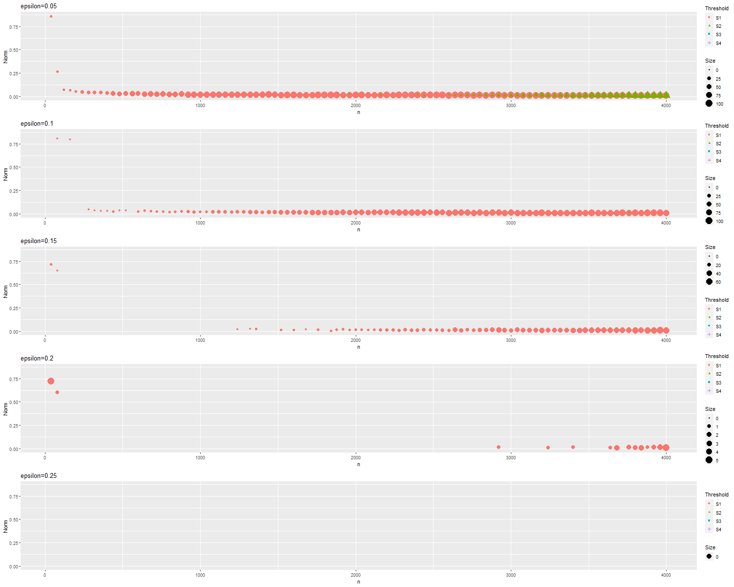
Refer to caption
Figure 7: Average estimate of the distance d(𝜽,𝜽^)superscript𝑑superscript𝜽^𝜽d^{\infty}\left(\boldsymbol{\theta}^{\star},\widehat{\boldsymbol{\theta}}\right) between the true parameters and the estimated parameters following ε𝜀\varepsilon (rows) in the arithmetic case: for each graphic, the threshold is represented by different symbols (\bullet for S1subscript𝑆1S_{1}, \blacktriangle for S2n,dsuperscriptsubscript𝑆2𝑛𝑑S_{2}^{n,d}, \blacksquare for S3n,dsuperscriptsubscript𝑆3𝑛𝑑S_{3}^{n,d} and +\boldsymbol{+} for S3n,dsuperscriptsubscript𝑆3𝑛𝑑S_{3}^{n,d}) and the size for the number of finite values used; the number of rows n𝑛n varies between 40 and 4000 and d𝑑d is supposed equal n𝑛n.
Refer to caption
Figure 8: On the left, boxplots of the computing times (in seconds; logarithmic scale) for each procedure (colour) in function of the numbers of rows and columns (n=d𝑛𝑑n=d) for each ε𝜀\varepsilon (in rows) over the 200 simulations for the balanced case. On the bottom, boxplots of quality of estimations averaged over the 20 matrices for each ε𝜀\varepsilon (in rows) for each procedure (colour) in function of the numbers of rows and columns (n=d𝑛𝑑n=d) for the balanced case.
Refer to caption
Figure 9: On the left, boxplots of the computing times (in seconds; logarithmic scale) for each procedure (colour) in function of the numbers of rows and columns (n=d𝑛𝑑n=d) for each ε𝜀\varepsilon (in rows) over the 200 simulations for the arithmetic case. On the bottom, boxplots of quality of estimations averaged over the 20 matrices for each ε𝜀\varepsilon (in rows) for each procedure (colour) in function of the numbers of rows and columns (n=d𝑛𝑑n=d) for the arithmetic case.

References

  • (1) Barbillon, P., Donnet, S., Lazega, E., Bar-Hen, A.: Stochastic block models for multiplex networks: an application to a multilevel network of researchers. Journal of the Royal Statistical Society: Series A (Statistics in Society) 180(1), 295–314 (2017)
  • (2) Bennett, J., Lanning, S.: The netflix prize. In: Proceedings of KDD cup and workshop, vol. 2007, p. 35 (2007)
  • (3) Biernacki, C., Celeux, G., Govaert, G.: Assessing a mixture model for clustering with the integrated completed likelihood. IEEE transactions on pattern analysis and machine intelligence 22(7), 719–725 (2000)
  • (4) Bouveyron, C., Latouche, P., Zreik, R.: The stochastic topic block model for the clustering of vertices in networks with textual edges. Statistics and Computing 28(1), 11–31 (2018)
  • (5) Brault, V., Keribin, C., Mariadassou, M., et al.: Consistency and asymptotic normality of latent block model estimators. Electronic journal of statistics 14(1), 1234–1268 (2020)
  • (6) Celeux, G., Chauveau, D., Diebolt, J.: On Stochastic Versions of the EM Algorithm. Rapport de recherche RR-2514, INRIA (1995). URL http://hal.inria.fr/inria-00074164
  • (7) Celisse, A., Daudin, J.J., Pierre, L., et al.: Consistency of maximum-likelihood and variational estimators in the stochastic block model. Electronic Journal of Statistics 6, 1847–1899 (2012)
  • (8) Channarond, A., Daudin, J.J., Robin, S., et al.: Classification and estimation in the stochastic blockmodel based on the empirical degrees. Electronic Journal of Statistics 6, 2574–2601 (2012)
  • (9) Govaert, G.: Classification croisée. Thèse d’état, Université Pierre et Marie Curie (1983)
  • (10) Govaert, G., Nadif, M.: Clustering with block mixture models. Pattern Recognition 36, 463–473 (2003)
  • (11) Hartigan, J.A.: Clustering Algorithms, 99th edn. John Wiley & Sons, Inc., New York, NY, USA (1975)
  • (12) Hedenfalk, I., Duggan, D., Chen, Y., Radmacher, M., Bitter, M., Simon, R., Meltzer, P., Gusterson, B., Esteller, M., Raffeld, M.: Gene-expression profiles in hereditary breast cancer. New Eng. J. Med. 344, 539–548 (2001)
  • (13) Iannario, M.: On the identifiability of a mixture model for ordinal data. Metron 68(1), 87–94 (2010)
  • (14) Jagalur, M., Pal, C., Learned-Miller, E., Zoeller, R.T., Kulp, D.: Analyzing in situ gene expression in the mouse brain with image registration, feature extraction and block clustering. BMC Bioinformatics 8(Suppl 10), S5 (2007)
  • (15) Keribin, C.: Cluster or co-cluster the nodes of oriented graphs? Journal de la société française de statistique 162(1), 46–69 (2021)
  • (16) Keribin, C., Brault, V., Celeux, G., Govaert, G.: Model selection for the binary latent block model. In: 20th International Conference on Computational Statistics. Limassol, Chypre (2012). URL http://hal.inria.fr/hal-00778145
  • (17) Keribin, C., Brault, V., Celeux, G., Govaert, G.: Estimation and selection for the latent block model on categorical data. Statistics and Computing pp. 1–16 (2014). DOI 10.1007/s11222-014-9472-2. URL http://dx.doi.org/10.1007/s11222-014-9472-2
  • (18) Laclau, C., Redko, I., Matei, B., Bennani, Y., Brault, V.: Co-clustering through optimal transport. In: International Conference on Machine Learning, pp. 1955–1964. PMLR (2017)
  • (19) Mariadassou, M., Matias, C., et al.: Convergence of the groups posterior distribution in latent or stochastic block models. Bernoulli 21(1), 537–573 (2015)
  • (20) Maugis, C., Michel, B.: A non asymptotic penalized criterion for gaussian mixture model selection. ESAIM: Probability and Statistics 15, 41–68 (2011)
  • (21) Mersmann, O.: microbenchmark: Accurate Timing Functions (2021). URL https://CRAN.R-project.org/package=microbenchmark. R package version 1.4.9
  • (22) Shan, H., Banerjee, A.: Bayesian co-clustering. In: Eighth IEEE International Conference on Data Mining, 2008. ICDM’08, pp. 530–539 (2008)
  • (23) Singh Bhatia, P., Iovleff, S., Govaert, G.: blockcluster: An R package for model-based co-clustering. Journal of Statistical Software 76(9), 1–24 (2017). DOI 10.18637/jss.v076.i09
  • (24) Tabouy, T., Barbillon, P., Chiquet, J.: Variational inference for stochastic block models from sampled data. Journal of the American Statistical Association 115(529), 455–466 (2020)
  • (25) Wyse, J., Friel, N.: Block clustering with collapsed latent block models. Statistics and Computing pp. 1–14 (2010)