Discovery and Modeling of a Flattening of the Positive Cyclotron Line/Luminosity Relation in GX 304$-$1 with RXTE

Abstract

The RXTE observed four outbursts of the accreting X-ray binary transient source, GX 304$-$1 in 2010 and 2011. We present results of detailed 3$-$100 keV spectral analysis of 69 separate observations, and report a positive correlation between cyclotron line parameters, as well as other spectral parameters, with power law flux. The cyclotron line energy, width and depth versus flux, and thus luminosity, correlations show a flattening of the relationships with increasing luminosity, which are well described by quasi-spherical or disk accretion that yield the surface magnetic field to be $\sim$60 keV. Since HEXTE cluster A was fixed aligned with the PCA field of view and cluster B was fixed viewing a background region 1.5 degrees off of the source direction during these observations near the end of the RXTE mission, the cluster A background was estimated from cluster B events using HEXTEBACKEST. This made possible the detection of the $\sim$55 keV cyclotron line and an accurate measurement of the continuum. Correlations of all spectral parameters with the primary 2$-$10 keV power law flux reveal it to be the primary driver of the spectral shape. The accretion is found to be in the collisionless shock braking regime.

1 INTRODUCTION

The study of neutron star magnetic fields in accreting X-ray pulsars has progressed significantly over the past few decades through the observations of cyclotron resonance scattering features (CRSFs), or cyclotron lines. Beginning with the discovery in 1976 of such a feature in Her X$-$1 (Trümper et al., 1978), we now have identified about two dozen accreting X-ray pulsars that exhibit cyclotron line features. The fundamental line energies range from 10 to 55 keV, implying magnetic field strengths from about 1 to 5 TG. Recent work to model the accretion column emission from a physics-based point of view is based upon the accreted material passing through a radiative, radiation dominated shock and forming a thermal mound just above the surface at the magnetic poles, as first proposed by Davidson (1973). Conditions in the infalling supersonic material are dominated by either radiation pressure at high luminosities or Coulomb interactions at lower luminosities before settling on the neutron star surface (e.g., Becker et al., 2012; Postnov et al., 2015b, and references therein). At the lowest luminosities no shock is formed and the material flows unabated until reaching the mound of material piled up on the magnetic poles. At high luminosities – defined as above the critical luminosity where radiation pressure dominates over gas pressure (Mushtukov et al., 2015a)– an increase in flux causes the shock, and thus the scattering region, to rise and sample lower magnetic field strengths, giving rise to a negative correlation of the cyclotron line energy with luminosity. Physically, the structure of accretion column starts changing with decreasing mass accretion rate when the photon diffusion time across the optically thick column becomes comparable to the matter settling time from the radiative shock height, and generally can be different in different sources. First estimates (e.g. Bakso & Sunyaev, 1976) shows it to be around $10^{37}$ erg s^-1 if the height of the radiative shock above the neutron star surface is comparable to the accretion column radius. With further decrease in the mass accretion rate onto the neutron star magnetic poles, the accretion flow decelerates most likely due to plasma instabilities leading to the formation of a collisionless shock, as numerical calculations performed at $\dot{M}<10^{1}6$ g s^s (e.g. Bykov & Krassilshchikov, 2004) suggest. The intermediate regime (i.e. between the radiative shock at high accretion rates and collisionless shock) is the most difficult to treatment, and still is to be explored numerically with taking into account the relevant complicated microphysics. In the collisionless shock regime, the height of the the scattering region decreases with increasing mass accretion rate thus producing a positive correlation of the cyclotron line with luminosity. Nishimura (2014) reproduces the same correlations with the line forming region being that between the top of the thermal mound and a height equal to twice the accretion column radius, both of which rise as the luminosity increases. Poutanen et al. (2013) have asserted a reflection model for the cyclotron line formation in which the shocked infalling matter generates X-rays that illuminate the atmosphere of the neutron star. In this case, increased accretion, and thus increased luminosity, increases the height of the X-ray emitting region and thus increases the area of the neutron star that is illuminated. This increased area contains lower values of the dipole magnetic field and thus the resulting cyclotron line has a lower value.

To date six accreting X-ray pulsars are known to have correlations of the fundamental cyclotron line energy with luminosity: one with a negative correlation, V 0332+53 (Tsygankov et al., 2006; Klochkov et al., 2011), and five with a positive correlation, Her X$-$1 (Staubert et al., 2007; Klochkov et al., 2011; Staubert et al., 2014, 2016), GX 304$-$1 (Klochkov et al., 2012), A 0535+26 (Klochkov et al., 2011), the first harmonic of Vela X$-$1 (Fürst et al., 2014), and Cep X$-$4 (Fürst et al., 2015). Note: 4U0115+63 is no longer deemed to have a correlation of the cyclotron line energy with luminosity (Müller et al., 2013; Boldin, Tsygankov & Lutovinov, 2013). La Parola et al. (2016) have recently published results from analysis of Swift/BAT observations of Vela X-1 where they find a positive correlation of the first harmonic cyclotron line energy with luminosity, and in addition, find a flattening of the correlation with increasing luminosity. Other spectral components, such as the power law index (e.g., Malacaria et al., 2015; Postnov et al., 2015b) and iron line flux, have been seen to vary with accretion rate as expressed by the X-ray flux.

GX 304$-$1 was first detected in a balloon flight (McClintock, Ricker & Lewin, 1971) and later by the Uhuru satellite as 2U1258-61 (Giacconi et al., 1972). It is an accreting neutron star exhibiting a teraGauss magnetic field in a high mass X-ray binary system with its companion B2Vne star, V850 Cen (Mason et al., 1978; Reig, Fabregat & Coe, 1997). The system has an orbital period of 132.1885$\pm$0.022 days (Sugizaki et al., 2015), a pulse period of $\sim$272 seconds (McClintock et al., 1977), and a distance of 2.4$\pm$0.5 kpc (Parkes, Murdin & Mason, 1980). After a nearly three decade period of quiescence, GX 304$-$1 emerged in 2008 (Manousakis et al., 2008), and began a series of regularly spaced outbursts in late 2009 (see fig. 1 of Yamamoto et al., 2011). A cyclotron resonance scattering feature at $\sim$54 keV was discovered during the 2010 August outburst (Yamamoto et al., 2011), and a possible positive correlation with flux was suggested. This has been confirmed with recent INTEGRAL results by Klochkov et al. (2012), who found the line varying between $\sim$48 keV and $\sim$55 keV, and by Malacaria et al. (2015) who found the range to be 50 to 59 keV with newer INTEGRAL calibrations. Four outbursts in 2010 and 2011 were observed by RXTE until its demise in 2012 January.

In this work we present an analysis of RXTE data of the outbursts in 2010 March/April, 2010 August, 2010 December/2011 January, and 2011 May, which represent 72 separate observations, of which 69 were analyzed in detail. From this we determine the variations of various spectral components with respect to unabsorbed power law flux, with which all are correlated. We present the Observations and Data Reduction in Section 2, Data Analysis in Section 3, Results in Section 4, and Discussion in Section 5, and present our conclusions in Section 6. In Appendix A we give the background and analysis that is the basis for the cluster A background estimation tool, HEXTEBACKEST. In Appendix B we give the tables of best-fit spectral parameters and plot them versus unabsorbed power law flux. Also in Appendix B we present representative contour plots of the cyclotron line parameters versus various spectral components. In Appendix C we discuss tests of the HEXTE background estimation and plot the systematic normalization constants.

2 OBSERVATIONS AND DATA REDUCTION

2.1 Observations

The Rossi X-ray Timing Exlorer (RXTE) observed GX 304$-$1 72 different times over its operational lifetime from 1996 to 2012, with three outbursts (2010 August, 2010 December, and 2011 May), numbering 69 observations, covered extensively. The outburst in 2010 March/April outburst had only 3 observations, and they are included to show consistency with the other outbursts. Three of the observations had less livetime than the GX 304-1 pulse period (Table 1 numbers 10, 52, and 62), and they were not included in subsequent analyses. Table 1 gives the dates, ObsIds, livetimes, and rates for both the Proportional Counter Array (PCA; Jahoda et al., 2006) Proportional Counter Unit 2 (PCU2) and for the High Energy X-ray Timing Experiment (HEXTE; Rothschild et al., 1998) Cluster A. Rates for PCU2 and HEXTE Cluster A are background subtracted. The sequential numbering of the individual observations is for identification in subsequent tables.

2.2 Data Reduction

PCA data were restricted to the 3$-$60 keV range of the top xenon layer of PCU2 due to the extensive calibration of this detector (Jahoda et al., 2006) that did not experience high voltage break down during the mission and thus were included in all PCA observations. The observational data were filtered to accept only observations with elevation above the Earth’s limb of greater than 10^∘, observation times more than 30 minutes from the start of the previous South Atlantic Anomaly passage, and electron rate below 0.5, instead of the nominal 0.1, due to the high X-ray flux adding counts to the electron detection portions of the proportional counter. The HEXTE data utilized the PCU2 filter criteria, were restricted to the 20$-$100 keV range, and data from both clusters were included in the analyses. The PCU2 background was estimated using PCABACKEST, and the PCU2 response was generated for the specific observation day using PCARSP. Due to rocking mechanism failures in the latter stages of the RXTE mission, HEXTE cluster A was continuously pointed on-source (after 2006 October 20), and cluster B was continuously pointed 1.5^∘ off-source (after 2009 December 12) to collect background data for all observations. The background spectrum for cluster A was then generated from that of cluster B using HEXTEBACKEST, as discussed in subsequent subsections and Appendix A. The cluster A spectral response was generated using HEXTERSP, which did not vary during the mission due to HEXTE’s automatic gain control.

The 3$-$60 keV PCU2, top layer, background subtracted, counting rates and the 20$-$100 keV HEXTE cluster A, background subtracted, counting rates for each of the three observing epochs are shown in panels a), b), and c) in Fig. 1. The HEXTE rates are multiplied by five in order to visually compare them with those of the PCU2. The 2010 August epoch observations cover from just before the maximum through decay to the beginning of a low state.

Table 1: RXTE Observations of GX 304$-$1

#	Date	ObsID	MJDa	PCA Lvtb	PCA Ratec	HEXTE Lvtb	HEXTE Rated
1	2010 Mar 27	95417-01-01-00	55282.34	2880	108.5$\pm$0.2	1620	13.7$\pm$0.3
2	2010 Mar 27	95417-01-01-01	55282.61	2192	114.1$\pm$0.2	1480	12.1$\pm$0.3
3	2010 Apr 6	95417-01-02-00	55292.68	3296	195.8$\pm$0.3	2275	69.8$\pm$0.3
4	2010 Aug 13	95417-01-03-03	55421.15	2304	997.4$\pm$0.7	1399	149.0$\pm$0.4
5	2010 Aug 13	95417-01-03-00	55421.20	3712	1060.2$\pm$0.5	2300	156.1$\pm$0.3
6	2010 Aug 14	95417-01-03-01	55422.07	5408	1125.0$\pm$0.5	1480	165.7$\pm$0.4
7	2010 Aug 15	95417-01-03-02	55423.09	6096	1212.4$\pm$0.4	1961	177.3$\pm$0.4
8	2010 Aug 18	95417-01-04-00	55426.10	3328	1197.0$\pm$0.6	184	190.5$\pm$1.1
9	2010 Aug 19	95417-01-04-01	55427.08	3216	1289.0$\pm$0.6	1966	178.0$\pm$0.4
10	2010 Aug 19	95417-01-04-02	55427.99	64	1470.0$\pm$4.8	33	186.3$\pm$2.9
11	2010 Aug 20	95417-01-05-00	55428.00	3120	1175.0$\pm$0.6	1922	161.1$\pm$0.4
12	2010 Aug 21	95417-01-05-01	55429.85	992	820.6$\pm$0.9	638	103.2$\pm$0.6
13	2010 Aug 23	95417-01-05-02	55431.00	2016	693.5$\pm$0.6	1159	84.0$\pm$0.4
14	2010 Aug 24	95417-01-05-03	55432.11	3408	578.7$\pm$0.4	2072	65.1$\pm$0.3
15	2010 Aug 25	95417-01-05-04	55433.24	1184	446.2$\pm$0.6	870	49.0$\pm$0.4
16	2010 Aug 26	95417-01-05-05	55434.03	1328	397.9$\pm$0.6	770	45.0$\pm$0.4
17	2010 Aug 27	95417-01-06-00	55435.26	1696	252.2$\pm$0.4	1234	29.0$\pm$0.3
18	2010 Aug 28	95417-01-06-01	55436.03	1984	188.3$\pm$0.3	1105	22.2$\pm$0.3
19	2010 Aug 29	95417-01-06-02	55437.35	1568	85.6$\pm$0.3	1108	16.2$\pm$0.4
20	2010 Aug 30	95417-01-06-03	55438.20	2336	58.2$\pm$0.2	1648	9.7$\pm$0.3
21	2010 Aug 31	95417-01-06-04	55439.07	1440	30.8$\pm$0.2	817	8.1$\pm$0.3
22	2010 Aug 31	95417-01-06-06	55439.13	1344	34.1$\pm$0.2	828	7.2$\pm$0.3
23	2010 Sep 1	95417-01-06-05	55440.75	832	22.9$\pm$0.2	543	6.8$\pm$0.4
24	2010 Dec 17	95417-01-07-00	55547.16	16400	162.1$\pm$0.1	10680	20.4$\pm$0.1
25	2010 Dec 19	95417-01-07-01	55549.83	2944	340.3$\pm$0.4	1793	40.8$\pm$0.3
26	2010 Dec 20	95417-01-07-02	55550.22	12210	315.9$\pm$0.2	7418	37.0$\pm$0.1
27	2010 Dec 21	95417-01-07-03	55551.27	7744	457.1$\pm$0.2	4651	57.4$\pm$0.2
28	2010 Dec 22	95417-01-07-04	55552.33	2848	698.7$\pm$0.5	1738	94.4$\pm$0.3
29	2010 Dec 23	95417-01-07-05	55553.12	8880	816.4$\pm$0.3	5625	81.6$\pm$0.3
30	2010 Dec 23	95417-01-07-06	55553.30	3664	756.6$\pm$0.5	2181	103.5$\pm$0.3
31	2010 Dec 23	95417-01-07-07	55553.37	3200	799.2$\pm$0.5	1807	110.7$\pm$0.3
32	2010 Dec 24	95417-01-08-00	55554.16	3408	827.8$\pm$0.5	2156	122.4$\pm$0.3
33	2010 Dec 25	95417-01-08-01	55555.07	3520	939.0$\pm$0.5	216	127.1$\pm$0.9
34	2010 Dec 26	95417-01-08-02	55556.18	3344	775.5$\pm$0.5	2016	112.5$\pm$0.3
35	2010 Dec 27	95417-01-08-03	55557.35	768	850.1$\pm$1.1	407	110.3$\pm$0.8
36	2010 Dec 28	95417-01-08-04	55558.27	2736	684.8$\pm$0.5	1592	88.9$\pm$0.3
37	2010 Dec 28	95417-01-08-05	55558.92	5760	692.5$\pm$0.4	3812	90.5$\pm$0.2
38	2010 Dec 29	95417-01-08-06	55559.92	5136	525.8$\pm$0.3	3295	67.2$\pm$0.2
39	2010 Dec 30	95417-01-08-07	55560.95	3344	412.6$\pm$0.4	2199	51.0$\pm$0.3
40	2011 Jan 1	96369-01-01-00	55562.80	9939	272.6$\pm$0.2	6471	31.9$\pm$0.1
41	2011 Jan 5	96369-01-01-01	55566.91	2524	28.5$\pm$0.1	1673	6.3$\pm$0.2
42	2011 Jan 8	96369-01-02-00	55569.59	1744	12.8$\pm$0.1	1105	7.1$\pm$0.3
43	2011 Jan 10	96369-01-02-01	55571.66	2544	16.1$\pm$0.1	1619	5.5$\pm$0.2
44	2011 Jan 12	96369-01-02-02	55573.82	2528	20.8$\pm$0.1	1496	5.7$\pm$0.2
45	2011 May 3	96369-01-03-00	55684.49	1280	633.2$\pm$0.7	866	81.4$\pm$0.4
46	2011 May 3	96369-01-03-01	55684.76	960	656.1$\pm$0.8	660	91.1$\pm$0.6
47	2011 May 4	96369-01-03-02	55685.00	1168	605.5$\pm$0.7	774	82.7$\pm$0.5
48	2011 May 4	96369-01-04-00	55685.53	1984	594.9$\pm$0.6	1387	74.3$\pm$0.3
49	2011 May 5	96369-01-05-00	55686.31	3584	565.2$\pm$0.4	2056	87.9$\pm$0.3
50	2011 May 5	96369-01-05-01	55686.44	6272	652.1$\pm$0.3	4313	96.2$\pm$0.2
51	2011 May 5	96369-01-05-02	55686.96	1136	621.1$\pm$0.8	749	91.4$\pm$0.5
52	2011 May 6	96369-02-01-00	55687.00	32	475.7$\pm$4.0	13	65.4$\pm$3.4
53	2011 May 6	96369-02-01-000	55687.00	17730	662.4$\pm$0.2	9977	104.0$\pm$0.1
54	2011 May 6	96369-02-01-02	55787.77	1056	1012.0$\pm$1.0	714	190.3$\pm$0.7
55	2011 May 6	96369-02-01-03	55687.84	768	732.2$\pm$1.0	514	125.9$\pm$0.7
56	2011 May 6	96369-02-01-04	55687.94	1104	568.1$\pm$0.07	738	94.0$\pm$0.5
57	2011 May 7	96369-02-01-01G	55688.00	18300	792.6$\pm$0.2	10000	126.6$\pm$0.1
58	2011 May 7	96369-02-01-05	55688.54	3072	986.9$\pm$0.6	830	152.4$\pm$0.5
59	2011 May 7	96369-02-01-06	55698.68	1344	806.9$\pm$0.8	919	131.2$\pm$0.5
60	2011 May 8	96369-01-06-00	55689.26	2064	1134.0$\pm$0.7	1131	180.8$\pm$0.5
61	2011 May 8	96369-01-06-01	55689.32	2912	974.5$\pm$0.6	1643	130.5$\pm$0.3
62	2011 May 9	96369-01-06-02	55690.27	96	845.3$\pm$3.0	51	134.6$\pm$2.1
63	2011 May 10	96369-01-06-03	55691.34	656	1289.0$\pm$1.4	433	187.3$\pm$0.8
64	2011 May 10	96369-01-06-04	55691.47	1344	947.1$\pm$0.8	962	127.0$\pm$0.5
65	2011 May 10	96369-01-07-00	55691.68	1728	875.5$\pm$0.7	1170	128.1$\pm$0.5
66	2011 May 11	96369-01-07-01	55692.25	4076	795.9$\pm$0.4	2372	101.2$\pm$0.3
67	2011 May 13	96369-01-08-00	55694.31	7056	457.2$\pm$0.3	4703	53.4$\pm$0.2
68	2011 May 14	96369-01-08-01	55695.29	1136	414.9$\pm$0.6	603	46.1$\pm$0.5
69	2011 May 15	96369-01-09-00	55696.34	3760	277.5$\pm$0.3	2544	29.5$\pm$0.2
70	2011 May 16	96369-01-09-01	55617.31	832	163.9$\pm$0.5	496	17.2$\pm$0.4
71	2011 May 17	96369-01-10-00	55698.40	3104	114.5$\pm$0.2	2165	16.0$\pm$0.2
72	2011 May 19	96369-01-10-01	55700.28	480	32.9$\pm$0.3	345	7.0$\pm$0.5

^a Start time of the observation
^b Livetime in seconds
^c 3$-$60 keV count rate in c/s
^d 20$-$100 keV count rate in c/s

The 2010 December epoch covers a full outburst from just after the start to well into the low state, but not reaching the peak intensities of the other two epochs. RXTE began observing the 2011 May epoch after it was well underway, similarly to that of the 2010 August epoch, and followed it to the low state. While all three light curves show similar decreases from peak values to a low state, the third epoch shows substantial counting rate variability approaching and at the peak of the outburst. As shown below, the majority of this variability is due to large variations in column density.

Systematics of 0.5% ($<$15 keV) and 1% (15$-$60 keV) were added to the PCU2 data for observations 5, 7, 8, 26, 29, 50, 53, 57, 60, and 61 to reduce the chi-square to an acceptable range for interpretation of parameter uncertainties. Addition of similar systematic errors to the other PCU2 data would have resulted in unreasonably low chi-square values in the spectral fitting. Otherwise, no systematic uncertainties were added to PCU2 data. No systematic uncertainties were added to the HEXTE data. In addition no spectral binning of either PCU2 or HEXTE-A data was used.

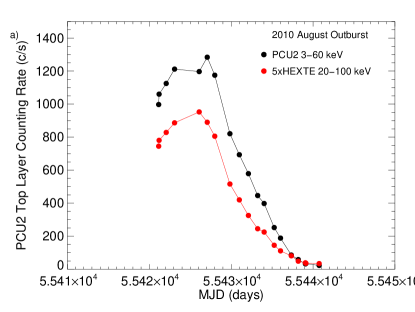
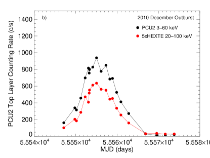
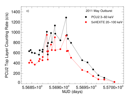
Figure 1: The PCU2 top layer 3$-$60 keV background subtracted, counting rates and the HEXTE cluster A 20$-$100 keV background subtracted, counting rates as a function of the observation date in Modified Julian Days. The 2010 August outburst is seen in panel a), the 2010 December outburst in panel b), and the 2011 May outburst in panel c). The PCU2 data are in black and the HEXTE data are in red. The HEXTE data have been multiplied by five.

3 DATA ANALYSIS

For each ObsID, the spectral histograms of PCU2 covering 3$-$60 keV and HEXTE cluster A covering 20$-$100 keV were simultaneously fit using ISIS 1.6.2-30 (Houck & Denicola., 2000), and verified with XSPEC 12.8.2 (Arnaud, 1996). For this analysis, two spectral models were utilized. The cutoffpl model approximated the continuum with a power law times an exponential to form a continuously steepening continuum, plus a blackbody (CUTOFFPL + BBODY), and the highecut model used a power law that abruptly changes to an exponentially falling continuum at a break energy (POWERLAW x HIGHECUT). Both models included low energy photoelectric absorption with interstellar abundances (TBnew). The abundances of Wilms, Allen & McCray (2000) and cross sections of Verner & Yakovlev (1995) were used in the analysis. The continuum was further modified by a Gaussian shaped cyclotron resonance scattering feature, or cyclotron line, (GAUABS) for those observations when the depth was measured, or had a lower limit, at greater than 90% confidence level. In addition, narrow ($\sigma$=10 eV), Gaussian line components were added fixed at 6.40 and 7.06 keV representing iron K$\alpha$ and K$\beta$ emission with the K$\beta$ flux set to 13% of the K$\alpha$ flux.

As presented in Appendix A, HEXTEBACKEST is based upon the channel by channel comparison of cluster A and cluster B background data for all of the observations in 2009 that included South Atlantic Anomaly passages. As such, the correlation parameters in each spectral bin are an average. Fig. 7 gives an idea of the spread in the data for two spectral channels. For any given observation, the correction factors will not give a cluster A background prediction that exactly expresses the background that would have been observed by cluster A, if it were rocking. Additionally, as the mission progressed from 2009, the satellite experienced lower and lower altitudes with the attendant increased magnetic rigidity and lesser South Atlantic Anomaly fluxes. This resulted in a somewhat lower background in the instruments. Consequently, four narrow Gaussians with fixed energies at 30.17, 39.04, 53.0, and 66.64 keV, representing corrections to the HEXTEBACKEST estimated fluxes of the four major HEXTE background lines were included in the modeling (see Appendix A for a description of HEXTEBACKEST and Appendix B for a presentation of the systematic lines versus 2$-$10 keV flux). The four energies were determined by averaging the individual fitted values during preliminary spectral analyses. The 30 keV and 67 keV lines are the strongest in the HEXTE background. While the lines at 39 keV and 53 keV are of lesser strength, they may affect the measurement of the energy of the known cyclotron line at $\sim$50-55 keV (Yamamoto et al., 2011), and were thus included in the fitting procedure.

The ‘10 keV feature’, which is seen in fits to accreting pulsar spectra (e.g., Coburn et al., 2002), was modeled by a negative Gaussian at 10.5 keV, when its inclusion reduced chi-square by 10 or more. No clear correlation was seen with respect to the detection of the 10 keV feature and power law flux. A systematic feature in the PCU2 fits occurs at about 3.88 keV in some of the observations, and it was modeled as a fixed energy, negative, narrow Gaussian, if the fitted depth was inconsistent with zero at the 90% confidence level.

The HEXTE model included the above mentioned parameters plus a constant representing the fractional difference in the response collecting area with respect to PCU2. The HEXTE constant was generally near 0.88, and was included in the variables of a given fitting procedure. Calculation of the PCU2 dead time showed that the deadtime correction was only a few percent at the highest PCU2 counting rates, and thus, no PCU2 deadtime correction was made. The HEXTE deadtime was calculated as an integral part of the data preparation using HEXTEDEAD. Since HEXTEDEAD is based upon average rates from two upper level discriminator rates (Rothschild et al., 1998), any individual observation may deviate from the average. Thus, to compensate for the few percent uncertainty of the PCA background and HEXTE background and deadtime models, the background subtractions were optimized with multiplicative parameters (RECOR in XSPEC and CORBACK in ISIS) during the fitting process. All uncertainties are expressed as 90% confidence.

The XSPEC model forms were:

F(E)=Recor*Const*TBnew*(Powerlaw*Highecut*Gauabs + Gauss(Fe_Kα) + Gauss(Fe_Kβ)) + Sys

or

F(E)=Recor*Const*TBnew*(Cutoffpl*Gauabs + Bbody + Gauss(Fe_Kα) + Gauss(Fe_Kβ)) + Sys

where

Sys = Gauss(3.88 keV) + Gauss(10.5 keV) + Gauss (30.17 keV) + Gauss(66.37 keV) + Gauss (39.04 keV) + Gauss (53.00 keV)

The best fit continuum parameters for all observations using the highecut and cutoffpl models are given in Appendix B as Tables 4 and 8. The best fit spectral line parameters are given in Tables 6 and 10. Plots of the various continuum parameters versus unabsorbed power law (highecut) or unabsorbed power law times exponential (cutoffpl) fluxes can be found in Appendix B and plots of the recor parameter and the HEXTE constant can be found in Appendix C. For those fittings where the search for the depth of the cyclotron line reached zero, no values for the cyclotron line parameters were reported and only double dashes are in Tables B1 and B2. For those fittings where a lower limit on the depth was found but not an upper limit, lower limits are given and values for the cyclotron line energy and width are given. Otherwise, both high and low limits are given. Examples of correlations between the fitted cyclotron line parameters and background lines at 53 keV and 66 keV, as well as versus the cutoff energy and folding energy of the continuum, are displayed in Appendix B for high and low flux observations #9 (12$\times 10^{-9}$ ergs cm^-2 s^-1) and #39 (4.7$\times 10^{-9}$ ergs cm^-2 s^-1) . In addition the correlation between the folding and cutoff energies is shown for those examples. At the lower flux levels, the correlation contours are somewhat bimodal and that the more significant maximum occurred for the higher value of the cyclotron line parameter.

As an example, the fit to ObsID 95417-01-04-01 is shown in Figure 2. The effects of excluding a cyclotron line component (panel b) and excluding the four HEXTE-A background lines (panel c) are shown as the ratio of the data to the model. Panel d) gives the ratio when all parameters are at their best-fit values. The reduced chi-square for this fit was 1.09 for 151 degrees of freedom. Note that the cyclotron line is clearly seen in the high energy portion of the PCU2 data (panel b), thus supporting the background estimation technique for HEXTE cluster A.

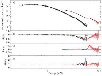
Figure 2: a): The PCU2 (black) and HEXTE-A (red) counts histogram for ObsID 95417-01-04-01 (2010 August 19) plotted versus energy. The best-fit model is the solid histogram in black. b): The residuals of the best-fit model with the depth of the cyclotron line set to zero. The residuals are expressed as the Ratio of the data to the model. c): The residuals to the best-fit HEXTE model with the four additional HEXTE-A background line fluxes set to zero. d): The residuals to the best-fit model with all parameters set to their best-fit values. The solid black line in the three Ratio residuals denotes a value of 1.

4 RESULTS

The two spectral models employed in the analysis generally lead to qualitatively similar results. From hereon throughout the rest of the paper, the highecut model results will be the subject of the discussion for two reasons. First, it has one parameter less than the cutoffpl model, and secondly, the continuum parameters do not influence each other to the degree that they do in the cutoffpl model, where the black body flux and the photon index are strongly correlated. This results in the parameters using the highecut model being better determined, such as the power law index and 2$-$10 keV continuum flux. The stable behavior of the column density at lower fluxes in the highecut model is preferred over the strong correlation with flux seen when modeling with the cutoffpl model. Section 4.3 gives a short discussion of the cutoffpl model fitting.

4.1 Peak Phase Zero Offsets

The orbital period of 132.1885$\pm$0.022 days (Sugizaki et al., 2015), and T₀=MJD 55554.75, determined from MAXI observations, were used to generate the respective orbital phases for each observation. The three sets of observations (now versus fitted 2$-$10 keV power law flux) have quite similar outburst decay profiles (Fig 3-a) with rise to peak flux and then decay to the lowest fluxes. By shifting the overall orbital phases slightly, the decay portions of the profiles align well (Fig. 3-b). The amounts of the peak epoch phase shifts were determined by first centering the midpoint of the peak of the 2010 December data on phase zero, since that outburst showed a relatively complete rise and fall of the flux. Then the remaining two data sets were shifted to align their falling portions to that of the 2010 December data. The resulting phase shifts are $-$0.045 for 2010 August, $-$0.010 for 2010 December, and $-$0.020 for 2011 May. These phase shifts amount to 5.9, 1.3, and 2.6 days earlier than the orbital period derived from the MAXI data would have suggested. This is consistent with the residual offsets from the orbital model in fig. 2 of Sugizaki et al. (2015) for these three outbursts covered by RXTE. This reveals that the shapes of the outbursts are quite similar once the flux drops below $\sim$10$\times 10^{-9}$ erg cm^-2 s^-1. The rising portions of the 2010 December and 2011 May outbursts also appear consistent with each other below $\sim$10$\times 10^{-9}$ erg cm^-2 s^-1. The first four 2010 August observations (black filled circles) may indicate that the 2010 August outburst exhibited an outburst with wider extent than the others, or was indicative of flaring during the rising portion of the outburst. The four 2011 May data points (red filled squares) above the common outburst trend are indicative of flaring near the peak of the 2011 May outburst. The three 2010 March/April points are not included here, since a phase shift could not be determined from so few points.

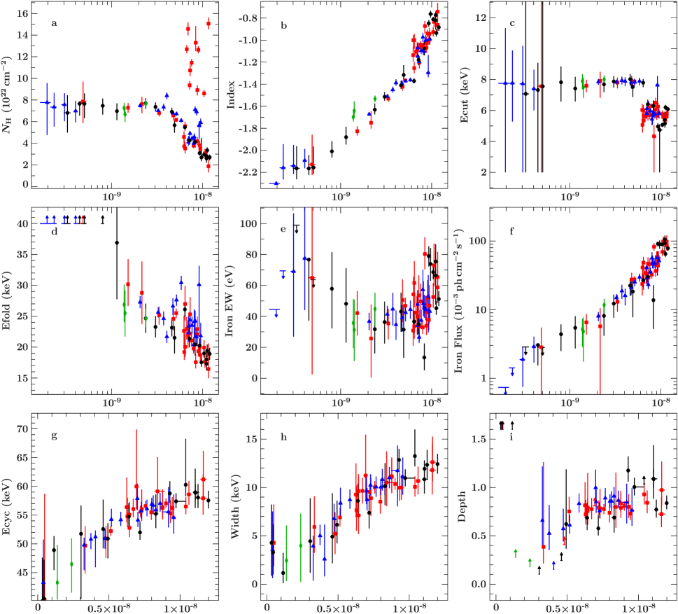
Figure 11: The continuum parameters for the highecut model plotted versus 2$-$10 keV unabsorbed flux in units of ergs cm^-2 s^-1. Data from 2010 March/April are in green, 2010 August are in black, 2010 December are in blue, and 2011 May are in red.

The flaring activity seen on the rising portion of the 2011 May outburst in Fig. 1, is absent in Fig. 3 and is attributable to the variation in column density affecting the PCU2 counting rate (see Fig. 11a). Individual points do remain above the overall outburst trend in Fig. 3, which may be considered flaring to some extent. Such flaring may be similar to the flaring activity seen on the rising portion of the 2005 August/September outburst of A0535$+$26 (Postnov et al., 2008; Caballero et al., 2008), and attributed to a low mode magnetospheric instability. These GX 304$-$1 data, however, do not show a significant change in the cyclotron line energy for any of the high flux points, whereas the A0535$+$26 data did, and other than the four earliest 2010 August outburst points, the points above the trend are at the maximum of the outbursts, and not on the rising edge, as in the 2005 August/September flares (Postnov et al., 2008; Caballero et al., 2008).

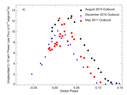
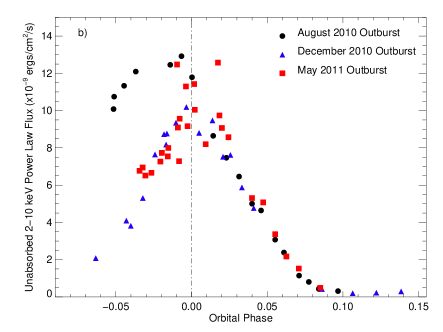
Figure 3: a: The unobscured power law 2$-$10 keV power law flux plotted versus orbital phase for the three outbursts in 2010 August, 2010 December, and 2011 May of GX 304$-$1, as observed by RXTE. b: The same data but with the orbital phases shifted by $-$0.045, $-$0.010, and $-$0.020, respectively, to match the 2010 August and 2011 May data to the falling portion of the 2010 December outburst. The 90% uncertainties are generally less than the size of the data points.

4.2 Variations with Power law Flux

Fig. 11 reveals that the highecut spectral parameters from the four outbursts have the same variations with power law flux and essentially the same values at any given flux level. Thus the accretion process for matter onto the neutron star was the same for all four outbursts.

A complete discussion of the column density variations is presented in Kühnel et al. (in preparation) where a large ($\times$3) column density enhancement event is detected in the 2011 May outburst (red points in Fig. 11a) and a smaller ($\times$0.5) enhancement is seen in the 2010 December data (blue points in Fig. 11a). These values associated with the large and small increases in column density are significant outliers from the overall trend of decreasing column density with increasing power law flux above a few 10^-9 ergs cm^-2 s^-1 and a constant value below that flux value.

The power law index has a strong positive correlation with power law flux (Fig. 11b). The four early 2010 August points noted earlier are now indistinguishable from the overall correlation with flux, which supports the contention that the flux is the primary driver of the continuum spectral shape. The continuum cut-off break energy (Fig. 11c) exhibits two distinct levels in the highecut model: $\sim$7.8 keV and $\sim$5.0$-$6.5 keV. The sharp transition from high to lower cut-off break energies appears at $\sim$6.5$\times 10^{-9}$ ergs cm^-2 s^-1, or (4.5$\pm$0.9)$\times 10^{36}$ ergs s^-1 for a distance of 2.4$\pm$0.5 kpc (Parkes, Murdin & Mason, 1980). The continuum folding energy shows an overall trend of decreasing energy with increasing power law flux (Fig. 11d).

The cyclotron line energy ($E_{\mathrm{cyc}}$; Fig. 11g) is found to range from 50 to 60 keV with an ever increasing value with power law flux in agreement with Klochkov et al. (2011). The widths ($W_{\mathrm{cyc}}$; Fig. 11h) vary with power law flux from 4 to 12 keV, and the depths ($\tau_{l}$; Fig. 11i) range from $\sim$1.1 down to $\sim$0.4, beyond which the depth is not significantly detected. For the cyclotron line energy and width, a positive correlation is clearly seen, while that for the depth or strength is less clear.

The iron line flux (Fig. 11f) shows a relatively smooth increase with flux. The iron line equivalent width variation with power law flux (Fig. 11e) was somewhat constant versus flux with large scatter between 2 and 4$\times 10^{-9}$ ergs cm^-2 s^-1 and at fluxes in excess of 10$\times 10^{-9}$ ergs cm^-2 s^-1.

4.3 Cutoffpl Fits

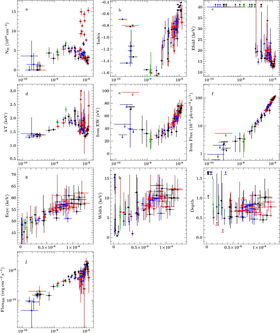
Figure 12: The continuum parameters for the cutoffpl model plotted versus 2$-$10 keV unabsorbed flux in units of ergs cm^-2 s^-1. The blackbody flux (Flux_BB) is in units of L₃₉/D², where L₃₉ is the flux in units of 10³⁹ ergs s^-1, and D is the distance to the source in units of 10 kpc. Data from 2010 March/April are in green, 2010 August are in black, 2010 December are in blue, and 2011 May are in red.

Fig. 12 shows the variation of spectral parameters with cutoff power law flux. Due to the shape of the cutoff power law and the blackbody component, the shape of the continuum is somewhat different than that of a straight power law. Therefore the values of the column density and power law index are slightly different than those from the highecut model. The column density still drops with increasing cutoff power law flux above $\sim 3\times 10^{-9}$ ergs cm^-2 s^-1 and the two column density enhancements are still above the trend. Where the highecut column density values leveled off at a value of $\sim 7\times 10^{22}$ cm^-2, those for cutoffpl drop to $\sim 3\times 10^{22}$ cm^-2 below $\sim 1\times 10^{-9}$ ergs cm^-2 s^-1. Similarly for the power law index, while highecut values have a linear series of values over the entire power law flux range, the cutoffpl values exhibit an abrupt change from the linear trend of the index at $\sim 1\times 10^{-9}$ ergs cm^-2 s^-1 to that of a constant value of $\sim$0.75 with large uncertainties. The blackbody temperature is constant at $\sim$1.1 keV from the lowest cutoff power law fluxes to $\sim 1\times 10^{-9}$ ergs cm^-2 s^-1, beyond which it rises linearly with flux to $\sim$2.7 keV. At ever-increasing cutoff power law flux, the trend is to decrease somewhat, albeit with large uncertainties. The cyclotron line parameters and the iron line fluxes variations are quite similar to those found in the highecut modeling.

4.4 Color/Intensity Diagrams

We have created the GX 304$-$1 soft (SC) and hard color (HC) versus intensity diagrams following the prescription of Reig & Nespoli (2013) with the intensity being the PCU2 4$-$30 keV count rate, the soft color being the ratio of the PCU2 4$-$7 keV to 7$-$10 keV count rates, and the hard color being the ratio of 15$-$30 keV to 10$-$15 keV rates. Fig 4a shows the SC versus intensity and Fig 4b the HC versus intensity. Both show increases in the color indices with increasing intensity, as expected for a hardening of the power law flux with intensity. For the SC/intensity diagram, the 2010 August and 2010 December outbursts follow the same track throughout their observations. The 2011 May outburst also follows the same track except for the period of time when the large column density enhancement was present. The larger column density values reduce the 4$-$7 keV fluxes and therefore raise the value of the soft color ratios. The hard color/intensity plot shows overlapping tracks for the three outbursts without the large deviations at higher intensity seen in the soft color plot, except for two of the the four last observations in 2010 December. The general trend of a reduction in soft and hard color indices throughout the outbursts can be attributed to the steepening of the power law component as the power law flux decreased, and the reversal of the hard color diagram below $\sim$100 counts per second may be attributable to the hardening of the spectrum at low fluxes as expressed in the spectral fitting by the increased values of E_fold. All together the soft and hard color/intensity diagrams imply that the accretion onto the neutron star was nearly identical in all three outbursts.

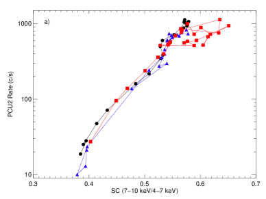
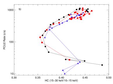
Figure 4: a: Soft color (7$-$10 keV/4$-$7 keV) plotted versus PCU2 4$-$30 keV counting rate for the three outbursts observed, following the prescription of Reig & Nespoli (2013). b: Hard color (15$-$30 keV/10$-$15 keV) plotted versus PCU2 4$-$30 keV counting rate.The colors for the three outbursts are the same as Fig 3.

4.5 Variance-Weighted Averages

Since we have demonstrated the nearly identical spectral performance in the four outbursts through the continuum parameters’ variations versus source flux and through the overlapping color intensity diagrams, we have performed a variance-weighted average of the power law index, cyclotron line energy and width, the iron line flux, and its equivalent width in six flux bins of width 2$\times 10^{-9}$ ergs cm^-2 s^-1 from zero to 12$\times 10^{-9}$ ergs cm^-2 s^-1 in order to reduce the scatter in parameter values and reduce uncertainties. The residual flux and cyclotron line depth values are given without the lowest flux bin since at most only lower limits were achieved.

The average CRSF energy, $\langle E_{\mathrm{cyc},i}\rangle$, in a certain flux bin, $i$, was found by minimizing the $\chi_{i}^{2}$ defined as

$$\chi_{i}^{2}=\sum_{k}\frac{(E_{\mathrm{cyc,k}}-\langle E_{\mathrm{cyc},i}\rangle)^{2}}{S(\sigma_{\mathrm{cyc,k}}^{+},\sigma_{\mathrm{cyc,k}}^{-})^{2}}$$ (1)

$\quad\text{with}\quad S=\begin{cases}\sigma_{\mathrm{cyc,k}}^{+}\quad\text{for~{}}E_{\mathrm{cyc,k}}-\langle E_{\mathrm{cyc},i}\rangle\leq 0,\\ \sigma_{\mathrm{cyc,k}}^{-}\quad\text{for~{}}E_{\mathrm{cyc,k}}-\langle E_{\mathrm{cyc},i}\rangle>0,\\ \end{cases}$

with the CRSF energy, $E_{\mathrm{cyc,k}}$, of each observation $k$ falling into the flux bin $i$, and the upper or the lower uncertainty, $\sigma_{\mathrm{cyc,k}}^{+}$ and $\sigma_{\mathrm{cyc,k}}^{-}$, of the CRSF energy. The average CRSF width ($W_{\mathrm{cyc,k}}$), depth ($\tau_{\mathrm{cyc,k}}$), and residual flux ($r=F_{\ell}(E_{\mathrm{cyc}})/F_{\mathrm{c}}(E_{\mathrm{cyc}})$) in each flux bin was found in the same way. The residual flux is related to the line ’optical depth’, $\tau_{\mathrm{\ell}}$, as $r=e^{-\tau_{\mathrm{\ell}}}$. Note that in case of symmetric uncertainties, i.e., $\sigma_{\mathrm{cyc,k}}^{+}$ = $\sigma_{\mathrm{cyc,k}}^{-}$, the average CRSF parameter value obtained is equivalent to the mean value weighted by the corresponding uncertainties (see, e.g., Bevington & Robinson, 1992).

The results are plotted in Fig. 5 where the cyclotron line parameters are in the lefthand panels and the power law index, iron line flux and equivalent width are in the righthand panels. All, except the residual flux, show positive correlations with flux, with the cyclotron line parameters gradually flattening with increasing flux. In Section 5.1 below, we show successful fits to the cyclotron line parameters with both disk accretion and quasi-spherical accretion models.

4.6 Comparison to Previous Observations

Yamamoto et al. (2011) presented spectral analyses of RXTE observations of the first two thirds of the 2010 August outburst, plus that of a Suzaku observation on 2010 August 13 after the second RXTE observation. Their analysis differed from that of the present work by only covering the 3$-$20 keV band in PCU2, using no extra Gaussians to augment hextebackest, ignoring the HEXTE band from 61$-$71 keV, and normalizing the PCU2 to HEXTE spectra by assuming no HEXTE flux above 150 keV. In addition, a different spectral model for the continuum, NPEX, was used. Nevertheless, they discovered the cyclotron line and concluded that the line had a positive correlation with overall flux or it had a bi-modal distribution. Cyclotron line energies ranged from 49$-$54 keV, albeit with large uncertainties on those values from lower luminosities. Klochkov et al. (2012) used 6 INTEGRAL observations covering the 2012 January outburst to confirm a positive correlation of the cyclotron line energy with flux employing the cutoffpl spectral model. The range of INTEGRAL cyclotron line energies was 48$-$ 55 keV. In the present work we have detected the cyclotron line in 54 of 69 observations, with individual energies ranging from 49 keV to 59 keV. Jaisawal, Naik & Eplil (2016) recently presented results from two Suzaku observations, one of which occurred at the time of the RXTE observations (4 & 5) on 2010 August 13. Their use of the NPEX and CYCLABS models for spectral fitting does not allow comparison to the present results due to the differing assumptions of spectral shapes. They did report, however, that the higher cyclotron line energies did occur for the brighter observation, as one would expect from the positive correlation with luminosity.

5 DISCUSSION

The present work covers three outbursts of GX 304$-$1 with twenty or more observations per outburst over a range of luminosities. The detailed modeling and corrections to the PCU2 background via the RECOR function and to the HEXTE background utilizing additional flux from the four prominent background lines in addition to HEXTEBACKEST plus RECOR has resulted in best-fit spectral parameters from spectra covering 3$-$100 keV with significant overlap in the 20$-$60 keV band, which allows for confirming the lower energy portions the HEXTE background subtraction.

5.1 Scaling Laws of CRSF Properties

The correlations of the CRSF properties with flux during outbursts of GX 304-1 suggest that the mass accretion rate onto the neutron star poles is the driver of the CRSF changes. The CRSF formation is a very complicated problem that can be solved only numerically by taking into account the dynamics of the accretion flow near the neutron star surface coupled with the radiation in the strong magnetic field. Qualitatively, however, it is clear that at low accretion rates, when the radiation field is not very strong, the braking of the flow is mediated by Coulomb interactions in the accreting plasma (e.g. Nelson, Salpeter & Wassermann (1993)), while at high accretion rates the flow is decelerated mostly due to interactions with photons (Davidson, 1973). The transition between these two extreme cases occurs gradually around some critical luminosity $\sim 10^{37}$ erg s^-1, which depends on the geometry of the flow and the structure of magnetic field near the neutron star surface and may be different in different sources (see Bakso & Sunyaev (1976), and more recent calculations in Becker et al. (2012), Mushtukov et al. (2015a)). At low luminosities, the CRSF energy in some sources (e.g. Her X-1) was found to positively correlate with X-ray flux, and in the simplest interpretation this can be due to a closer location of the effective site of CRSF formation with respect to the neutron star surface, where the magnetic field is stronger, with increasing mass accretion rate (Staubert et al., 2007). Clearly, with increasing X-ray luminosity, transition to the radiation-dominated regime occurs, where the effective height of accretion column gets higher, and hence the CRSF energy is expected to decrease with increasing X-ray flux, as indeed observed in some bright transient X-ray pulsars (e.g. V0332+53, Tsygankov et al. (2006)). La Parola et al. (2016) make similar assumptions in the fitting of the Vela X-1 first harmonic positive correlation of cyclotron line energy with luminosity.

Here we suggest a possible interpretation of the observed correlations in GX 304-1, assuming that the source, even at the highest X-ray flux in the outburst, is indeed well below the critical luminosity (Becker et al., 2012), which implies it remains in the regime where the radiation effects are subdominant in braking the accretion flow. This will enable us to use the results of detailed calculations of the (effectively one-dimensional in this case) plasma flow above the neutron star surface. In this way we will obtain simple formulae that can be used to fit the observed correlations of the CRSF energy, $E_{\mathrm{cyc}}$, its width, $W$, the line residual flux, $r$, and its related line optical depth $\tau_{\ell}$ with changing X-ray flux (see Table 2).

5.1.1 Physical setup

In the GX 304$-$1 case, the accretion flow decelerates in a collisionless shock (Langer & Rappaport, 1982). The height of the collisionless shock above the neutron star surface, $H_{\mathrm{s}}$, is governed by energy exchange between protons (which tap most of the post-shock energy) and electrons, and the cooling of electrons and ions via bremsstrahlung and cyclotron losses; photons participate in the post-shock dynamics of the flow via resonant and non-resonant scattering on electrons in the strong magnetic field, but their density is insufficient to produce a radiation-dominated shock (Bykov & Krassilshchikov, 2004). With increasing mass accretion rate, $H_{\mathrm{s}}$ decreases because the plasma density increases, and the line formation region within the cyclotron resonant layer downstream of the shock gets closer to the neutron star surface. The CRSF formation is governed by the resonance electron scattering of thermal photons produced at the base of the accretion mound where most of the free-fall energy is released. Thus, the scaling with mass accretion rate appears for the line centroid energy, its width, residual flux, and depth.

A photon with energy $\hbar\omega$ experiences resonant scattering on an electron at the fundamental cyclotron resonance frequency $\omega_{\mathrm{cyc}}$ in the magnetic field $B$, and $E_{\mathrm{cyc}}=\hbar\omega_{\mathrm{cyc}}=\hbar eB/(m_{\mathrm{e}}c)$, where $e$ is the electron charge, $m_{\mathrm{e}}$ is the electron mass, and $c$ is the speed of light. Therefore, in the plasma above the neutron star surface, for each photon of energy $E$ there should be the cyclotron resonance scattering radius, $r_{\mathrm{res}}=R_{\mathrm{NS}}((\hbar eB_{\mathrm{NS}}/m_{\mathrm{e}}c)/E)^{1/3}$, due to inhomogeneity of the dipole magnetic field, $B=B_{\mathrm{NS}}(R_{\mathrm{NS}}/r)^{3}$, where $R_{\mathrm{NS}}$ is the neutron star radius and $B_{\mathrm{NS}}$ is the surface magnetic field at the magnetic pole (Zheleznyakov, 1996).

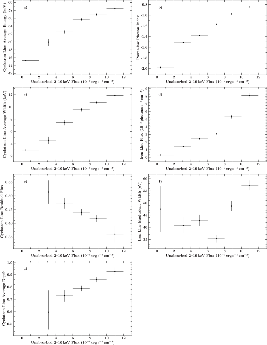
Figure 5: The variance weighed average cyclotron line energies (a), power law indices (b), cyclotron line widths (c), iron line flux (d), cyclotron line residual fluxes (e), iron line equivalent widths (f), and cyclotron line average depth (g) in six 2$-$10 keV, unabsorbed, power law flux bins for the energy and width of the cyclotron lines, and in five flux bins for the residual flux and the depth.

As shown in Zheleznyakov (1996), the width of the resonant layer for the assumed dipole magnetic field is $\Delta r_{\mathrm{res}}\sim\beta_{T_{\mathrm{e}}}r_{\mathrm{res}}/3$, where $\beta_{T_{\mathrm{e}}}=v_{T_{\mathrm{e}}}/c\sim 1/10$ is the thermal velocity of post-shock electrons; for typical temperatures $T_{\mathrm{e}}\sim 10$ keV and $\hbar\omega_{\mathrm{cyc}}\sim 50$ keV, $\Delta r_{\mathrm{res}}\sim 6\times 10^{4}$ cm can be comparable with the shock size $H_{\mathrm{s}}$ and thus can substantially modify the CRSF formation. Note that the post-shock electron temperature $T_{\mathrm{e}}$ does not vary substantially. The characteristic optical depth of the resonant layer in the inhomogeneous dipole magnetic field $B$ is (Zheleznyakov, 1996)

$$\tau_{\mathrm{res}}=\frac{16}{3}\frac{\pi^{2}e^{2}}{m_{\mathrm{e}}c}\frac{n_{\mathrm{e}}\Delta r_{\mathrm{res}}}{\omega_{\mathrm{cyc}}}\sim\\ 10^{4}\left(\frac{n_{\mathrm{e}}}{10^{20}\mathrm{cm}^{-3}}\right)\left(\frac{50\,\mathrm{keV}}{E_{\mathrm{cyc}}}\right)^{\frac{4}{3}}\left(\frac{R_{\mathrm{NS}}}{10^{6}\mathrm{cm}}\right)\left(\frac{B_{\mathrm{NS}}}{10^{12}\mathrm{G}}\right)^{\frac{1}{3}}\,.$$ (2)

It is also known that during the cyclotron resonance scatterings the number of scatterings of a photon in the resonant layer scales as the optical depth, $N_{\mathrm{sc}}\propto\tau_{\mathrm{res}}$, in contrast to the scaling $N_{\mathrm{sc}}\propto\tau^{2}$ for the non-resonance Thomson scattering (Wasserman & Saltpeter, 1980; Lyutikov & Gavriil, 2006; Garasev et al., 2011). This has an important consequence for the CRSF discussed below.

Table 2: Fitting formulae for the CRSF centre energy, $E_{\mathrm{cyc}}$, width $W$, the residual line flux $r$ and line optical depth $\tau_{\ell}$ as a function of X-ray flux $F_{\mathrm{x}}$ in the collisionless shock braking regime, assuming a magnetospheric radius $R_{\mathrm{m}}\sim M^{-x}$

Formula	$x_{\mathrm{d}}=2/7$	$x_{\mathrm{s}}=2/11$
$E_{\mathrm{cyc}}(F_{\mathrm{x}})=E_{0}(K_{1}F_{\mathrm{x}}^{-\alpha}+1)^{-3}$	$\alpha_{\mathrm{d}}=5/7$	$\alpha_{\mathrm{s}}=9/11$
$W(F_{\mathrm{x}})=K_{2}E_{\mathrm{cyc}}^{1/3}(F_{\mathrm{x}})F_{\mathrm{x}}^{\beta}$	$\beta_{\mathrm{d}}=5/14$	$\beta_{\mathrm{s}}=9/22$
$r(F_{\mathrm{x}})=K_{3}E_{\mathrm{cyc}}^{2/3}(F_{\mathrm{x}})F_{\mathrm{x}}^{-\gamma}$	$\gamma_{\mathrm{d}}=5/14$	$\gamma_{\mathrm{s}}=9/22$
$\tau_{\ell}(F_{\mathrm{x}})=K_{4}+\ln\left(E_{\mathrm{cyc}}^{-2/3}(F_{\mathrm{x}})F_{\mathrm{x}}^{\gamma}\right)$	$\gamma_{\mathrm{d}}=5/14$	$\gamma_{\mathrm{s}}=9/22$

The height of the collisionless shock is $H_{\mathrm{s}}\sim(v_{0}/4)t_{\mathrm{eq}}\propto 1/n_{\mathrm{e}}$ (here $t_{eq}$ is the electron-proton equilibration time; see e.g. Shapiro & Salpeter, 1975). The electron number density behind the shock can be estimated from the mass continuity equation

$${}n_{\mathrm{e}}=\left(\frac{\dot{M}}{A}\right)\left(\frac{4}{v_{0}m_{\mathrm{p}}}\right)\,.$$ (3)

The accretion area $A$ is determined by the magnetospheric radius $R_{\mathrm{m}}$ and for the dipole field should vary as $A\sim(R_{\mathrm{NS}}\sqrt{R_{\mathrm{NS}}/R_{\mathrm{m}}})^{2}\propto 1/R_{\mathrm{m}}$. In the general case, the magnetospheric radius is inversely proportional to the mass accretion rate, $R_{\mathrm{m}}\propto\dot{M}^{-x}$, where $x=x_{\mathrm{d}}=2/7$ for disc accretion or Bondi quasi-spherical accretion, or $x=x_{\mathrm{s}}=2/11$ for quasi-spherical settling accretion (Shakura et al., 2012), where the latter may be realized in the case of GX 304-1 (Postnov et al., 2015a).

With these scalings, we find for the electron number density $n_{\mathrm{e}}\propto\dot{M}/A\propto\dot{M}^{1-x}$. Therefore, the characteristic shock height scales with accretion rate as

$$H_{\mathrm{s}}\propto 1/n_{\mathrm{e}}\propto A/\dot{M}\propto\dot{M}^{-\alpha}\,,$$ (4)

and $n_{\mathrm{e}}\propto\dot{M}^{\alpha}$, where $\alpha=\alpha_{\mathrm{d}}=1-x_{\mathrm{d}}=5/7$ for disc or Bondi quasi-spherical accretion and $\alpha=\alpha_{\mathrm{s}}=1-x_{\mathrm{s}}=9/11$ for quasi-spherical settling accretion.

5.1.2 Cyclotron line energy scaling with X-ray flux

Consider the case where the characteristic size of the plasma region, $H_{\mathrm{s}}\lesssim 10^{5}$ cm, is comparable with the thickness of the resonant layer, $\Delta r_{\mathrm{res}}\sim 6\times 10^{4}$ cm. The optical depth of the resonant layer is very large (see Eq. (2)). The CRSF is formed at some effective energy corresponding to the magnetic field at some height within the resonance layer, which is related to the shock height, $H_{\mathrm{CRSF}}\lesssim H_{\mathrm{s}}$, and hence should have the same dependence on the mass accretion rate as H_s. The CRSF energy is $E_{\mathrm{cyc}}\propto B(R)\propto 1/R^{3}$, and noticing that $R=R_{\mathrm{NS}}+H_{\mathrm{CRSF}}$, we find, for the assumed dipole magnetic field,

$${E_{\mathrm{cyc}}(\dot{M})}=E_{0}\left(\frac{R_{\mathrm{NS}}}{H_{\mathrm{CRSF}}(\dot{M})+R_{\mathrm{NS}}}\right)^{3}\,,$$ (5)

where $E_{0}$ corresponds to the line emitted from the NS surface magnetic field $B_{\mathrm{NS}}$. Clearly, the line dependence on the observed X-ray flux is entirely determined by how the collisionless shock height $H_{\mathrm{s}}$ responds to the variable mass accretion rate (see Eq. (4) above). As the observed X-ray flux $F_{\mathrm{x}}$ is directly proportional to $\dot{M}$ and introducing the relation $H_{\mathrm{CRSF}}/R_{\mathrm{NS}}=K_{1}F_{\mathrm{x}}^{-\alpha}$, we arrive at

$$E_{\mathrm{cyc}}(F_{\mathrm{x}})=E_{0}(K_{1}F_{\mathrm{x}}^{-\alpha}+1)^{-3}\,.$$ (6)

The constant $K_{1}$, which determines the CRSF location height, $H_{\mathrm{CRSF}}/R_{\mathrm{NS}}$, can be found from fitting the observational data, $\alpha_{d}$=5/7 and $\alpha_{s}$=9/11. Generally, $K_{1}$ may be a function of $\dot{M}$ as well, but in view of lack of solid theory of CRSF formation downstream the shock we will assume $K_{1}=const$.

5.1.3 Cyclotron line width scaling with X-ray flux

As discussed above, the resonant line is formed by multiple scatterings in a resonant layer behind the shock. In each single scattering on an electron, moving essentially in one dimension along the magnetic field lines, the energy of the resonant photon is Doppler shifted, $(\Delta E_{\mathrm{cyc}}/E_{\mathrm{cyc}})_{1}=\pm\beta_{T_{\mathrm{e}}}$, where the post-shock electron temperature $T_{\mathrm{e}}\sim 10$ keV does not strongly vary in the scattering region. Therefore, after many scatterings the CRSF width will be $W/E_{\mathrm{cyc}}\simeq\sqrt{(\Delta E_{\mathrm{cyc}}/E_{\mathrm{cyc}})_{1}^{2}N_{\mathrm{sc}}}\propto\sqrt{T_{\mathrm{e}}N_{\mathrm{sc}}}\propto\sqrt{N_{\mathrm{sc}}}\propto\sqrt{\tau_{\mathrm{res}}}$. As follows from Eq. (2), $\tau_{\mathrm{res}}\propto n_{\mathrm{e}}/E_{\mathrm{cyc}}^{4/3}$, and hence the observed CRSF width can be fitted by the following formula:

$$W(F_{\mathrm{x}})=K_{2}E_{\mathrm{cyc}}^{1/3}(F_{\mathrm{x}})F_{\mathrm{x}}^{\beta}\,,$$ (7)

where $\beta=\alpha/2$, $E_{\mathrm{cyc}}(F_{\mathrm{x}})$ is determined by formula (6) and $K_{2}$ is a constant.

5.1.4 Cyclotron line residual flux and line ‘depth’ scaling with X-ray flux

Finally, we consider how the residual flux at the line center changes with X-ray luminosity in our model. Consider the simplest case of an isothermal atmosphere with resonance scattering (the Eddington model), which can be a good first approximation for the resonant layer behind the collisionless shock front. It is easy to check that in our case with $E_{\mathrm{cyc}}=\hbar\omega_{\mathrm{cyc}}\sim 50$ keV $\gg kT_{\mathrm{e}}\sim$ 10 keV and with typical densities $n_{\mathrm{e}}\sim 10^{20}$ cm^-3, the ratio of the absorption to scattering is very small, i.e. we can neglect absorptions of scattered photons altogether. According to the theory of resonance scattering lines in an isothermal atmosphere (see, e.g., Ivanov, 1969, (chapter 7)), and (Ivanov, 1973), in the limit of high survival probability of scattered photons in the continuum and neglecting the absorption, the residual flux $r$ of a resonance line (the so-called ’$\lambda$-solution’) is determined solely by the number of scatterings of the line photons and scales as

$$r=\frac{1}{\sqrt{N_{\mathrm{sc}}}}\propto\frac{1}{\sqrt{\tau_{\mathrm{res}}}}\propto\frac{E_{\mathrm{cyc}}^{2/3}}{\sqrt{n_{\mathrm{e}}}}\,.$$ (8)

Plugging in the scaling $n_{\mathrm{e}}\propto\dot{M}^{\alpha}$, we can recast this expression into the convenient form:

$$r(F_{\mathrm{x}})=K_{3}E_{\mathrm{cyc}}^{2/3}(F_{\mathrm{x}})F_{\mathrm{x}}^{-\gamma}\,,$$ (9)

where $K_{3}$ is a constant and $\gamma=\alpha/2$, yielding $\gamma_{\mathrm{d}}=5/14$ and $\gamma_{\mathrm{s}}=9/22$ for disc and quasi-spherical accretion, respectively.

It is also possible to introduce the line ‘optical depth’ $\tau_{\ell}$ defined as $r=e^{-\tau_{\ell}}$. It is this parameter that is usually inferred from data analysis. The application of formula  (9) in this case is straightforward:

$$\tau_{\ell}(F_{\mathrm{x}})=K_{4}+\ln(E_{\mathrm{cyc}}^{-2/3}(F_{\mathrm{x}})F_{\mathrm{x}}^{\gamma})\,,$$ (10)

where $K_{4}$ is the constant to be found from fitting. (Note that the fitting procedure of $\tau_{\ell}(F_{\mathrm{x}})$ should be done independently of fitting $r(F_{\mathrm{x}})$, since these quantities are derived independently from the data analysis.)

5.1.5 Fitting the Variance-weighted Data

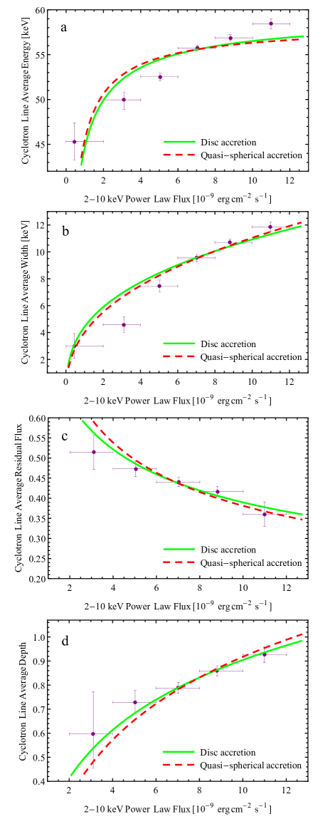
Figure 6: Best-fits of the observed cyclotron line parameters versus X-ray flux for two possible types of accretion in GX 304-1, disc or quasi-spherical, shown by solid green line and dashed red line, respectively. a) Cyclotron line energy (6); b) cyclotron line width (7); c) cyclotron line residual flux (9); and d) cyclotron line ’depth’ (10). Horizontal bars indicate the width of the flux bins inside which averaging was done.

The results of fitting the variance-weighted data (described in section 4.5 and shown in Fig. 5) by formulae  (6),  (7),  (9), and  (10) are shown in Fig. 6 and listed in Table 3. We do not show formal errors in the fitting coefficients due to roughness of the model physical assumptions (constant electron temperature, approximate treatment of the cyclotron resonance scattering, etc.). It is also seen that the data do not allow us to distinguish between the two possible dependences of the magnetospheric radius on $\dot{M}$ for different types of accretion (disc or quasi-spherical one).

Table 3: Best-fit parameters of $E_{\rm cyc}(F_{\rm x})$, $W(F_{\rm x})$, $r(F_{\rm x})$ and $\tau_{\ell}(F_{\rm x})$

Param	Disc accretion	Quasi-spherical accretion
Fig. 6a: fit $E_{\rm cyc}(F_{\rm x})$ by Eq. (6)
$E_{0}$	$59.99$	$58.62$
$K_{1}$	$0.1$	$0.09$
Fig. 6b: fit $W(F_{\rm x})$ by Eq. (7)
$K_{2}$	$1.25$	$1.12$
Fig. 6c: fit $r(F_{\rm x})$ by Eq. (9)
$K_{3}$	$0.06$	$0.07$
Fig. 6d: fit $\tau_{\ell}(F_{\rm x})$ by Eq. (10)
$K_{4}$	$2.77$	$2.66$

$E_{0}$ is energy in keV
$K_{1}$ is flux^α ($10^{-9\alpha}$ erg^α cm^-2α s^-α)
$K_{2}$ is energy^2/3 flux^-β (keV^2/3 10^9β erg^-β cm^2β s^β)
$K_{3}$ is energy^-2/3 flux^γ (keV^-2/3 10^-9γ erg^γ cm^-2γ s^-γ)
$K_{4}$ is dimensionless

With further increase in accretion rate, the transition to radiation braking regime and the appearance of an optically thick accretion column should occur (Bakso & Sunyaev, 1976). The critical luminosity for the transition is expected near $10^{37}$erg s^-1 (Becker et al. 2012, see also Mushtukov et al. 2015a for recent more accurate calculations). While the brightest single observation only reached $\sim(7\pm 1.4)\times 10^{36}$ erg s^-1 for the 2.4$\pm$0.5 kpc of Parkes et al. (1980), it would be interesting to probe the transition between different accretion regimes in transient X-ray pulsars with more powerful outbursts.

Note that an alternative explanation of the positive correlations between $E_{\mathrm{cyc}}-F_{\mathrm{x}}$ and $W-F_{\mathrm{x}}$ at moderate X-ray luminosities was recently proposed by Mushtukov et al. (2015b). However, that model predicts the opposite sign of the second derivative in the $E_{\mathrm{cyc}}-F_{\mathrm{x}}$ and $W-F_{\mathrm{x}}$ relations (cf. black solid lines in Fig. 6a and 6b Fig. 7a in Mushtukov et al., 2015b), while the simple physical explanation given above is consistent with observations of GX 304$-$1.

5.2 Outburst Shifts in Orbital Phase

The shifts in orbital phase applied to the three outbursts can be understood in terms of changes in the size of the circumstellar disk around V850 Cen. Referring to Fig. 4 in Postnov et al. (2015a), the disk is inclined with respect to the orbital plane of the neutron star, and the neutron star passes through the disk at point A, accumulating matter that forms a temporary accretion disk (Devasia et al., 2011). The lack of a double peak to the three outbursts implies that the circumstellar disk does not extend to the recrossing of the line of nodes at point B. Changes in the thickness of the circumstellar disk from one orbit to the next will affect the amount of matter captured in the accretion disk and thus the duration of the outburst. The few percent orbital phase shifts imply small variations in the circumstellar disk on timescales of a hundred days.

5.3 Flux Correlation in General

The strong positive correlations of spectral parameters with source flux, clearly indicate that the source flux, or indeed the mass accretion rate, is responsible for the overall continuum shape and that of the cyclotron line as well. This is also supported by the nearly identical soft color/intensity curves for the three outbursts and the fact that the four early 2010 August observations yield consistency with other observations when plotted versus flux as opposed to plotted versus orbital phase. Kühnel et al. (2013) similarly found that the key driver for the continuum shape in GRO J1008$-$57 was the power law flux. They found a common spectral model based on flux independent parameters and flux correlations for three Type I outbursts and a Type II outburst, where the power law flux was the defining variable, when the source was in the subcritical state.

5.4 Soft Color versus Flux

We find that the soft color ratio increases with increasing flux along the horizontal branch (Reig & Nespoli, 2013), with excursions from the overall track due to an extra amount of material in the line of sight over about 3 days. The hard color ratio shows a similar horizontal branch increase with intensity, but also shows a reversal of the trend at the lowest intensities. The changes in the soft and hard color ratios with intensity can be related to the overall steepening of the power law index with decreasing intensity and its hardening of the falling exponential at the lowest intensities. The flattening of spectra with increasing X-ray flux, as is seen in Fig. 4, could be due to increase in the optical depth inside the scattering region behind the shock and hence in the $y$-parameter in the unsaturated Comptonization regime.

6 CONCLUSIONS

This work presents the analysis of RXTE observations of the accreting X-ray pulsar GX 304$-$1 that provides the finest detail to date on the correlation of the cyclotron line parameters (energy, width, depth, and residual flux) with source flux for any accreting X-ray binary system. The correlations display, for the first time, a flattening with increasing power law flux. This is successfully modeled by a rather simple one-dimensional physical treatment of both disk accretion and quasi-spherical accretion, since in this case no optically thick accretion column is assumed to form above the neutron star polar caps, and the emergent radiation is thus dynamically unimportant. The neutron star surface magnetic field is measured to be $\sim$60 keV in both models. In addition, the correlations of the power law index, break energy, and iron line flux with power law flux points strongly to the source flux, and thus the mass accretion rate, as the overarching determinant of the spectral behavior.

Appendix A HEXTEBACKEST

(This section is based upon the poster “Estimating the HEXTE A Background Spectrum”, which was presented at the 9th AAS HEAD meeting, Pottschmidt et al., 2006). Since the launch of RXTE in 1995, the HEXTE instrument mostly operated in its standard ‘rocking’ mode where the pointing direction of each of its two clusters alternated between source and background measurements in such a way that one cluster was always looking at the source while the other sampled the background. During the extraction of source light curves and spectra, each cluster uses its own background measurements for correction. This allowed HEXTE to achieve signal to background ratios of <1% for long observations ($\gtrsim$400 ks) of weak sources (Rothschild et al., 1998). Starting in 2005 December the rocking mechanism of cluster A began to display increasingly frequent interruptions and since 2006 July was permanently fixed in the on-source staring position. We have developed a FTOOL, HEXTEBACKEST, which for a given observation uses the background measured by cluster B to produce an estimated cluster A background spectrum. The tool uses a set of channel dependent parameters to perform a linear transformation of the count rates. We explain how these parameters were derived, compare estimated and measured cluster A backgrounds for archived rocking observations, and present examples of the application of the method. Cluster B began experiencing similar rocking interruptions in 2009 December and was permanently fixed in one of the off-source positions at the end of 2010 March. This enabled cluster B to collect background data for use with HEXTEBACKEST to estimate cluster A background for the rest of the RXTE mission.

A.1 Introduction

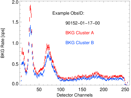
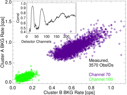
Figure 7: Left: Background spectrum measured by HEXTE’s clusters A (red) and B (blue) for AO9 observation ObsID 90152-01-17. Note that there is an instrumental cutoff below channel $\sim 10$ and above channel $\sim 246$ (starting from 0). Right: Cluster A versus cluster B background rates measured in channels 70 (purple) and 100 (green) for 3570 ObsIDs of AO9. The inset shows the correlation coefficient between the A and B rates for all channels based on these observations.

Both clusters used their off-source observations to measure their individual backgrounds, which are different from each other mainly but not only due to the fact that cluster B had only 3 operating detectors after 1996 March. For an example of the measured background spectra, see top panel of Fig. 7. The cluster A background can be estimated based on the measured cluster B background: their rates are well correlated for each detector channel (inset of bottom panel of Fig. 7, with varying correlation coefficients which become especially high in the background lines around 30 and 70 keV [detector channels $\sim$ energy channels for HEXTE]). We extracted the background spectra of several thousand exposures performed during the ninth mission year (AO9, 2004). Fig. 7-bottom panel demonstrates the correlation in two selected channels, one associated with a peak in the spectrum and one not.

A.2 Linear Correction Parameters

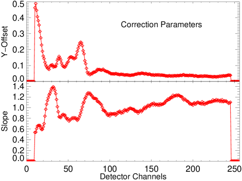
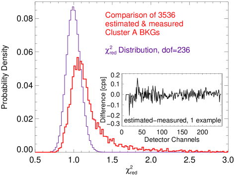
Figure 8: Left:Results of linear fits, $rate\_A=m(channel)\times rate\_B+\Delta y(channel)$, for 3570 ObsIDs. Left, Above: Offset $\Delta y$. Left, Below: Slope $m$. Both parameters have been set to $0$ for channels below 10 and above 246. Right: $\chi^{2}$ comparison of the estimated and measured cluster A backgrounds for the AO9 ObsIDs (red). The theoretical distribution is also shown (purple). The inset shows the difference between the estimated and measured cluster A backgrounds for one typical observation.

We performed linear fits to the A versus B background rates for each detector channel based on the AO9 data set using poly_fit in IDL and taking A and B uncertainties into account. Note that the 3570 ObsIDs are the result of pre-selection: (1) observations with high A or B rates in the lower channels have been omitted to screen against sources in the background field of view, (2) since observations performed far from the SAA show different background correlations, they have also been omitted. The top panel in Fig. 8 shows the correction parameters we obtained. In the bottom panel of Fig. 8, the estimated and measured cluster A spectra are compared (red) – the former based on the AO9 cluster B measurements and on the correlation parameters – using the statistic $\chi^{2}_{\text{red}}=\sum[d^{2}/(\sigma_{\text{est}}^{2}+\sigma_{\text{meas}}^{2})]/$dof for each observation, where $d$ is the estimated minus the measured cluster A background spectrum, $\sigma_{\text{est}}$ and $\sigma_{\text{meas}}$ are the spectral uncertainties, and the number of valid channels, dof (degrees of freedom), is 236 (see Bevington & Robinson 1992, for comparing two independent data sets). With respect to the theoretical distribution (purple) a small shift and a tail of higher $\chi^{2}$ values can be seen.

A.3 Applications

The method outlined above is available to derive HEXTE cluster A background spectra for post-2006 July observations. Each HEASOFT release contains the FTOOL HEXTEBACKESTwhich takes an input .pha file, performs the linear correction for all channels, and writes a corrected output .pha file. A FITS file with the correction parameters is part of the calibration database (CALDB), distributed from NASA’s High Energy Science Archive and Research Center (HEASARC). As a hidden parameter of HEXTEBACKEST it will by default be remotely accessed. See ‘fhelp hextebackest’ for more details (e.g., on spectral binning). Here we show that for recent observations of bright sources the estimated cluster A background gives satisfactory results in the sense that the same source fits as with the measured cluster A backgrounds are obtained applying systematic uncertainties of 2% or less. Limited tests with spectra from AO4 and earlier show that the correction parameters are not adequate for older observations. Fig. 9 shows the comparison between the measured cluster A background and that generated by hextebackest for one example observation. Deviations between the two data sets are mostly seen at the peaks of the stronger background lines. HEXTEBACKEST was applied for the observation of a smooth continuum (Cyg X$-$1; Fig. 10-left) and one with two cyclotron line features imposed on the continuum (V0332+653; Fig. 10-right). In both cases the residuals to the fit are shown for the case of estimated and measured backgrounds, and they are comparable in both cases. This demonstrates that the HEXTEBACKEST does not introduce spurious features in the spectra.

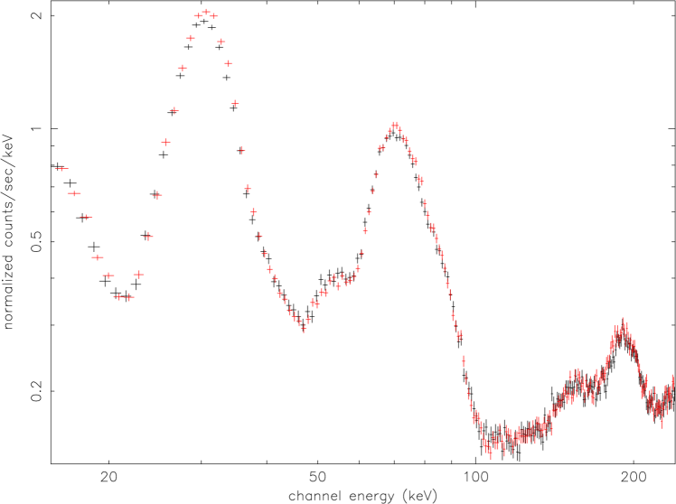
Figure 9: Estimated (red) and measured (black) cluster A background for the Cyg X-1 observation shown in Fig. 10. As confirmed by the source fit the estimated background is a good match, however, small deviations, especially in the line peaks, remain.

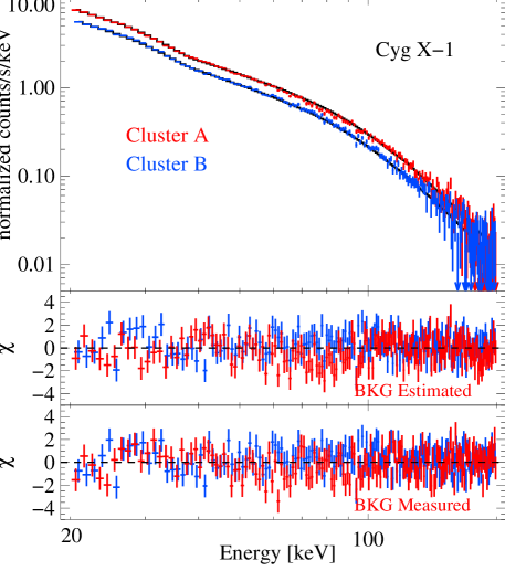
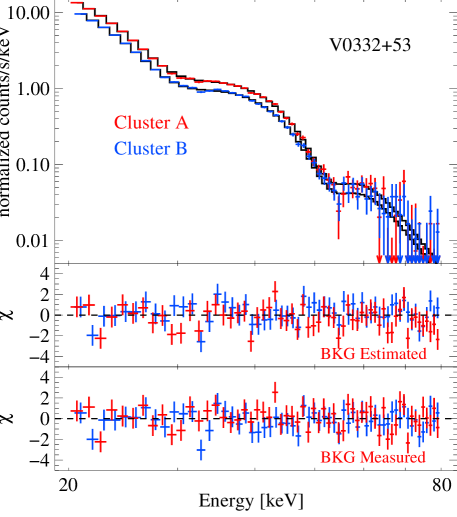
Figure 10: Left, Top: HEXTE cluster A (red) and B (blue) counts spectra with the best fit cutoffpl model (black) for an observation of the black hole binary Cyg X-1 performed on 2004 Nov. 30. The spectrum has been averaged over 5 ObsIDs. The spectrum used for the cluster A background subtraction has been estimated based on the cluster B background and the correction parameters. Left, Middle: Residuals using the estimated cluster A background, best fit parameters: $\Gamma=1.53^{+0.02}_{-0.02}$, $E_{\text{cut}}=132^{+8}_{-7}$ keV, $K=1.22^{+0.07}_{-0.07}$  photons/keV/cm²/s at 1 keV. Left, Bottom: Residuals using the measured cluster A background, best fit parameters: $\Gamma=1.54^{+0.02}_{-0.02}$, $E_{\text{cut}}=134^{+8}_{-7}$ keV, $K=1.25^{+0.07}_{-0.07}$  photons/keV/cm²/s at 1 keV. The two fits thus lead to consistent results without applying additional systematics in order to take uncertainties in the cluster A background estimate into account. Right, Top: HEXTE cluster A (red) and B (blue) counts spectra with the best fit two-cyclotron-lines model (black) for an observation of the transient pulsar V0332$+$53 performed on 2004 Dec. 12. The spectrum used for the cluster A background subtraction has been estimated based on the cluster B background and the correction parameters. Right, Middle: Residuals using the estimated cluster A background, best fit parameters: $\Gamma=-0.15^{+0.75}_{-0.57}$, $E_{\text{cycl1}}=28.83^{+0.08}_{-0.07}$ keV, $E_{\text{cycl2}}=51.5^{+0.6}_{-0.6}$ keV. Right, Bottom: Residuals using the measured cluster A background, best fit parameters: $\Gamma=+0.50^{+0.51}_{-0.55}$, $E_{\text{cycl1}}=28.83^{+0.08}_{-0.07}$ keV, $E_{\text{cycl2}}=51.3^{+0.6}_{-0.6}$ keV. The two fits thus lead to consistent results, in this case, however, systematics of 2% had to be applied in order to take uncertainties in the cluster A background estimate into account.

Appendix B Spectral Fit Tables and Figures

This section contains the best fit parameters from the spectral fitting of each observation with both the highecut and cutoffpl models. The tables are divided into the continuum and the line parameters. After the tables, plots of the various parameters are given.

Table 4: Best-fit Highecut Continuum Spectral Parameters of GX 304$-$1

#	$N_{\mathrm{H}}^{a}$	Indexb	Fluxc	Ecutd	Efoldd	Ecyce	Widthe	Depthe	$\chi^{2}$/dof
1	$7.30^{+0.50}_{-0.60}$	$1.700^{+0.050}_{-0.060}$	$1.377^{+0.028}_{-0.030}$	$7.90^{+0.50}_{-0.60}$	$26.90^{+3.30}_{-2.90}$	$43.30^{+6.60}_{-3.00}$	$2.40^{+3.70}_{-2.20}$	$\geq 0.28$	1.22/152
2	$6.70^{+0.60}_{-0.80}$	$1.640^{+0.060}_{-0.090}$	$1.410^{+0.040}_{-0.050}$	$7.50^{+0.70}_{-0.70}$	$25.00^{+4.00}_{-4.00}$	$--$	$--$	$--$	1.04/155
3	$7.70^{+0.40}_{-0.40}$	$1.533^{+0.028}_{-0.031}$	$2.380^{+0.040}_{-0.040}$	$8.01^{+0.28}_{-0.30}$	$24.60^{+1.60}_{-1.50}$	$46.00^{+5.00}_{-5.00}$	$4.00^{+4.00}_{-4.00}$	$0.37^{+6.48}_{-0.19}$	1.20/152
4	$3.10^{+0.23}_{-0.23}$	$0.848^{+0.030}_{-0.029}$	$9.280^{+0.080}_{-0.080}$	$4.96^{+0.24}_{-0.26}$	$20.30^{+1.20}_{-1.00}$	$58.80^{+2.20}_{-1.70}$	$12.90^{+1.20}_{-1.00}$	$1.18^{+0.15}_{-0.12}$	1.18/151
5	$2.70^{+1.90}_{-0.40}$	$0.760^{+0.040}_{-0.040}$	$9.720^{+0.680}_{-0.130}$	$4.70^{+0.40}_{-2.80}$	$17.50^{+0.90}_{-0.80}$	$57.40^{+1.40}_{-1.20}$	$11.00^{+1.00}_{-0.90}$	$1.00^{+0.10}_{-0.09}$	0.89/151
6	$2.94^{+0.21}_{-0.16}$	$0.811^{+0.031}_{-0.022}$	$10.400^{+0.090}_{-0.060}$	$5.07^{+0.15}_{-0.15}$	$19.00^{+1.30}_{-0.70}$	$60.30^{+8.00}_{-2.10}$	$\geq 12.2$	$1.16^{+0.69}_{-0.13}$	1.24/151
7	$2.80^{+0.40}_{-0.40}$	$0.770^{+0.040}_{-0.040}$	$11.080^{+0.130}_{-0.120}$	$5.14^{+0.27}_{-0.26}$	$18.00^{+0.90}_{-0.80}$	$58.90^{+1.60}_{-1.30}$	$11.90^{+0.90}_{-0.80}$	$1.09^{+0.11}_{-0.09}$	0.87/152
8	$2.60^{+0.60}_{-0.40}$	$0.820^{+0.090}_{-0.060}$	$11.070^{+0.260}_{-0.170}$	$5.40^{+0.60}_{-0.40}$	$17.30^{+2.00}_{-1.10}$	$59.00^{+4.10}_{-2.80}$	$10.80^{+2.00}_{-1.50}$	$1.09^{+0.35}_{-0.21}$	1.01/153
9	$2.71^{+0.27}_{-0.29}$	$0.880^{+0.040}_{-0.040}$	$11.990^{+0.120}_{-0.140}$	$6.08^{+0.16}_{-0.19}$	$18.90^{+1.00}_{-1.00}$	$57.50^{+1.70}_{-1.40}$	$12.40^{+1.10}_{-1.00}$	$0.84^{+0.08}_{-0.07}$	1.09/151
11	$3.36^{+0.27}_{-0.30}$	$0.940^{+0.040}_{-0.040}$	$11.260^{+0.120}_{-0.130}$	$6.20^{+0.17}_{-0.19}$	$19.40^{+1.10}_{-1.10}$	$58.10^{+2.40}_{-1.90}$	$12.30^{+1.60}_{-1.50}$	$0.77^{+0.11}_{-0.09}$	1.25/152
12	$4.10^{+0.60}_{-0.60}$	$1.080^{+0.070}_{-0.070}$	$8.300^{+0.170}_{-0.180}$	$6.30^{+0.40}_{-0.40}$	$20.40^{+2.20}_{-1.90}$	$55.20^{+3.40}_{-2.50}$	$10.10^{+2.40}_{-2.00}$	$0.69^{+0.19}_{-0.16}$	0.75/152
13	$4.30^{+0.40}_{-0.40}$	$1.180^{+0.050}_{-0.050}$	$7.190^{+0.120}_{-0.110}$	$6.40^{+0.31}_{-0.26}$	$21.40^{+1.80}_{-1.50}$	$52.00^{+1.90}_{-1.30}$	$7.40^{+1.90}_{-1.70}$	$0.58^{+0.14}_{-0.08}$	0.88/152
14	$5.49^{+0.21}_{-0.23}$	$1.371^{+0.021}_{-0.027}$	$6.400^{+0.060}_{-0.060}$	$7.80^{+0.24}_{-0.30}$	$26.10^{+1.10}_{-1.20}$	$54.70^{+2.40}_{-1.70}$	$8.60^{+1.80}_{-1.60}$	$0.69^{+0.16}_{-0.13}$	1.01/152
15	$5.70^{+0.50}_{-0.70}$	$1.320^{+0.060}_{-0.090}$	$4.930^{+0.100}_{-0.140}$	$7.50^{+0.60}_{-0.70}$	$21.50^{+1.90}_{-2.60}$	$50.90^{+2.70}_{-3.50}$	$6.10^{+2.50}_{-2.00}$	$0.62^{+0.57}_{-0.26}$	0.93/152
16	$6.90^{+0.40}_{-0.40}$	$1.410^{+0.040}_{-0.040}$	$4.600^{+0.070}_{-0.070}$	$8.00^{+0.40}_{-0.50}$	$23.10^{+1.50}_{-1.50}$	$53.00^{+6.00}_{-4.00}$	$4.90^{+4.50}_{-2.80}$	$0.60^{+5.40}_{-0.40}$	0.78/152
17	$7.40^{+0.50}_{-0.50}$	$1.510^{+0.040}_{-0.050}$	$3.040^{+0.050}_{-0.060}$	$7.90^{+0.40}_{-0.40}$	$23.30^{+1.80}_{-1.70}$	$52.00^{+5.00}_{-12.00}$	$4.00^{+5.00}_{-4.00}$	$\geq 0.10$	1.01/152
18	$7.70^{+0.50}_{-0.60}$	$1.630^{+0.050}_{-0.060}$	$2.370^{+0.050}_{-0.060}$	$7.70^{+0.50}_{-0.60}$	$24.70^{+2.40}_{-2.40}$	$--$	$--$	$--$	1.19/155
19	$7.00^{+0.80}_{-0.90}$	$1.880^{+0.070}_{-0.100}$	$1.150^{+0.040}_{-0.050}$	$7.40^{+0.80}_{-0.90}$	$37.00^{+14.00}_{-10.00}$	$48.90^{+2.50}_{-3.50}$	$1.20^{+2.10}_{-1.10}$	$\geq 0.18$	1.23/151
20	$7.50^{+0.70}_{-0.90}$	$2.010^{+0.060}_{-0.100}$	$0.801^{+0.026}_{-0.032}$	$7.80^{+1.10}_{-1.30}$	$48.00^{+23.00}_{-14.00}$	$--$	$--$	$--$	0.96/155
21	$7.66^{+0.00}_{-1.11}$	$2.160^{+0.060}_{-0.130}$	$0.447^{+0.000}_{-0.024}$	$7.30^{+1.80}_{-5.40}$	$\geq 44.8$	$41.00^{+7.00}_{-4.00}$	$3.30^{+2.90}_{-2.30}$	$\geq 0.67$	1.08/153
22	$7.70^{+1.00}_{-1.40}$	$2.160^{+0.060}_{-0.200}$	$0.504^{+0.026}_{-0.037}$	$8.00^{+13.00}_{-6.00}$	$\geq 38.0$	$--$	$--$	$--$	0.84/155
23	$6.80^{+1.70}_{-1.90}$	$2.160^{+0.100}_{-0.210}$	$0.328^{+0.027}_{-0.029}$	$7.00^{+13.00}_{-6.00}$	$\geq 32.5$	$40.00^{+8.00}_{-4.00}$	$4.00^{+4.00}_{-4.00}$	$\geq 0.21$	0.97/153
24	$7.47^{+0.17}_{-0.18}$	$1.672^{+0.016}_{-0.018}$	$2.060^{+0.015}_{-0.016}$	$7.85^{+0.20}_{-0.21}$	$27.30^{+1.00}_{-1.00}$	$--$	$--$	$--$	1.85/154
25	$8.40^{+0.30}_{-0.32}$	$1.388^{+0.027}_{-0.033}$	$4.050^{+0.050}_{-0.050}$	$7.89^{+0.26}_{-0.31}$	$21.70^{+1.00}_{-1.10}$	$51.20^{+1.20}_{-5.30}$	$2.60^{+3.60}_{-1.80}$	$\geq 0.15$	0.67/152
26	$7.30^{+0.40}_{-0.40}$	$1.450^{+0.026}_{-0.028}$	$3.740^{+0.050}_{-0.050}$	$7.94^{+0.25}_{-0.27}$	$24.60^{+1.20}_{-1.20}$	$50.80^{+1.10}_{-1.70}$	$5.00^{+1.20}_{-1.00}$	$0.53^{+0.30}_{-0.18}$	0.98/152
27	$6.72^{+0.17}_{-0.18}$	$1.371^{+0.016}_{-0.019}$	$5.170^{+0.040}_{-0.040}$	$7.83^{+0.20}_{-0.23}$	$27.60^{+0.90}_{-1.00}$	$54.30^{+1.90}_{-1.30}$	$8.40^{+1.60}_{-1.40}$	$0.61^{+0.11}_{-0.09}$	1.06/152
28	$4.10^{+0.40}_{-0.40}$	$1.070^{+0.040}_{-0.050}$	$7.000^{+0.090}_{-0.100}$	$5.79^{+0.24}_{-0.30}$	$22.30^{+1.40}_{-1.50}$	$57.90^{+2.60}_{-2.10}$	$9.60^{+1.50}_{-1.40}$	$1.00^{+0.19}_{-0.15}$	1.13/153
29	$4.00^{+0.40}_{-0.40}$	$0.970^{+0.050}_{-0.040}$	$8.010^{+0.120}_{-0.110}$	$5.40^{+0.40}_{-0.40}$	$20.40^{+1.30}_{-1.10}$	$56.90^{+1.20}_{-1.00}$	$10.00^{+0.90}_{-0.90}$	$0.86^{+0.08}_{-0.07}$	0.98/152
30	$4.44^{+0.28}_{-0.30}$	$1.100^{+0.040}_{-0.040}$	$7.670^{+0.090}_{-0.100}$	$5.97^{+0.21}_{-0.24}$	$23.50^{+1.50}_{-1.50}$	$56.10^{+1.60}_{-1.40}$	$10.10^{+1.10}_{-1.10}$	$0.89^{+0.11}_{-0.10}$	1.11/152
31	$4.60^{+0.40}_{-0.50}$	$1.090^{+0.050}_{-0.070}$	$8.110^{+0.120}_{-0.150}$	$5.70^{+0.40}_{-0.60}$	$24.10^{+2.00}_{-2.60}$	$56.70^{+1.80}_{-1.50}$	$10.80^{+1.10}_{-1.20}$	$0.86^{+0.11}_{-0.10}$	1.11/152
32	$6.90^{+0.40}_{-0.40}$	$1.000^{+0.040}_{-0.050}$	$8.600^{+0.110}_{-0.120}$	$5.77^{+0.23}_{-0.30}$	$21.70^{+1.40}_{-1.50}$	$57.00^{+1.80}_{-1.50}$	$11.00^{+1.20}_{-1.10}$	$0.87^{+0.11}_{-0.08}$	1.01/152
33	$5.90^{+0.40}_{-0.50}$	$0.990^{+0.050}_{-0.070}$	$9.550^{+0.150}_{-0.170}$	$5.81^{+0.26}_{-0.33}$	$21.80^{+2.20}_{-2.10}$	$54.60^{+4.00}_{-2.90}$	$11.10^{+2.10}_{-1.90}$	$0.76^{+0.24}_{-0.17}$	1.19/151
34	$7.10^{+0.30}_{-0.32}$	$1.100^{+0.040}_{-0.050}$	$8.290^{+0.100}_{-0.110}$	$5.83^{+0.25}_{-0.30}$	$24.20^{+1.70}_{-1.70}$	$55.90^{+1.40}_{-1.20}$	$10.10^{+1.00}_{-1.00}$	$0.91^{+0.10}_{-0.09}$	0.90/152
35	$5.60^{+0.50}_{-1.30}$	$1.300^{+0.050}_{-0.170}$	$9.180^{+0.140}_{-0.440}$	$7.60^{+0.60}_{-1.40}$	$30.00^{+4.00}_{-8.00}$	$55.50^{+4.40}_{-2.70}$	$11.70^{+2.60}_{-3.70}$	$0.85^{+0.20}_{-0.22}$	0.85/152
36	$4.40^{+0.40}_{-0.40}$	$1.150^{+0.040}_{-0.050}$	$7.040^{+0.100}_{-0.100}$	$6.12^{+0.25}_{-0.27}$	$23.40^{+1.70}_{-1.60}$	$54.10^{+1.50}_{-1.20}$	$8.70^{+1.30}_{-1.20}$	$0.85^{+0.13}_{-0.12}$	0.95/152
37	$4.91^{+0.23}_{-0.23}$	$1.197^{+0.028}_{-0.028}$	$7.280^{+0.070}_{-0.070}$	$6.43^{+0.20}_{-0.18}$	$24.40^{+1.40}_{-1.20}$	$55.70^{+1.70}_{-1.40}$	$10.20^{+1.20}_{-1.10}$	$0.76^{+0.09}_{-0.08}$	1.06/152
38	$6.11^{+0.18}_{-0.19}$	$1.362^{+0.017}_{-0.020}$	$5.830^{+0.040}_{-0.050}$	$7.89^{+0.22}_{-0.27}$	$30.40^{+1.20}_{-1.20}$	$54.20^{+1.40}_{-1.10}$	$8.70^{+1.10}_{-1.00}$	$0.83^{+0.11}_{-0.10}$	1.19/152
39	$6.79^{+0.26}_{-0.29}$	$1.395^{+0.024}_{-0.032}$	$4.730^{+0.050}_{-0.060}$	$7.82^{+0.29}_{-0.36}$	$26.60^{+1.30}_{-1.50}$	$50.90^{+1.60}_{-1.80}$	$6.80^{+1.60}_{-1.40}$	$0.57^{+0.21}_{-0.14}$	0.78/152
40	$7.02^{+0.17}_{-0.18}$	$1.512^{+0.016}_{-0.017}$	$3.260^{+0.022}_{-0.023}$	$7.83^{+0.17}_{-0.18}$	$25.60^{+0.90}_{-0.90}$	$49.80^{+1.30}_{-4.40}$	$3.90^{+1.10}_{-3.60}$	$0.66^{+0.56}_{-0.28}$	1.15/152
41	$7.00^{+1.00}_{-1.10}$	$2.090^{+0.080}_{-0.110}$	$0.403^{+0.019}_{-0.020}$	$7.40^{+1.30}_{-1.40}$	$\geq 33.8$	$43.00^{+8.00}_{-6.00}$	$3.60^{+4.00}_{-3.00}$	$\geq 0.56$	1.13/153
42	$7.80^{+1.80}_{-3.10}$	$2.300^{+0.140}_{-0.590}$	$0.196^{+0.019}_{-0.033}$	$8.00^{+4.00}_{-6.00}$	$\geq 19.6$	$--$	$--$	$--$	1.20/156
43	$7.30^{+1.40}_{-1.90}$	$2.160^{+0.110}_{-0.220}$	$0.234^{+0.016}_{-0.021}$	$7.80^{+2.20}_{-2.50}$	$\geq 24.8$	$--$	$--$	$--$	0.88/156
44	$7.60^{+1.10}_{-1.60}$	$2.140^{+0.080}_{-0.190}$	$0.304^{+0.016}_{-0.023}$	$7.70^{+2.50}_{-5.80}$	$\geq 35.4$	$--$	$--$	$--$	0.90/156
45	$3.70^{+0.60}_{-0.40}$	$1.000^{+0.100}_{-0.050}$	$6.300^{+0.160}_{-0.090}$	$5.10^{+0.70}_{-0.50}$	$19.20^{+2.90}_{-1.30}$	$54.80^{+3.30}_{-1.90}$	$7.60^{+2.60}_{-2.20}$	$0.72^{+0.15}_{-0.11}$	0.96/152
46	$3.50^{+0.60}_{-0.50}$	$1.000^{+0.080}_{-0.060}$	$6.440^{+0.160}_{-0.110}$	$5.30^{+0.50}_{-0.40}$	$20.00^{+2.70}_{-1.70}$	$52.80^{+3.70}_{-1.60}$	$7.10^{+4.00}_{-2.00}$	$0.79^{+0.36}_{-0.18}$	0.87/153
47	$4.60^{+0.60}_{-0.70}$	$1.140^{+0.060}_{-0.080}$	$6.260^{+0.130}_{-0.150}$	$6.00^{+0.40}_{-0.60}$	$22.60^{+2.50}_{-2.50}$	$56.40^{+5.20}_{-2.70}$	$9.30^{+3.30}_{-2.40}$	$0.82^{+0.25}_{-0.14}$	1.02/153
48	$5.60^{+0.50}_{-0.50}$	$1.250^{+0.050}_{-0.060}$	$6.430^{+0.120}_{-0.120}$	$6.00^{+0.40}_{-0.50}$	$27.00^{+3.00}_{-2.70}$	$55.10^{+2.30}_{-1.70}$	$9.60^{+1.80}_{-1.80}$	$0.76^{+0.14}_{-0.08}$	0.95/152
49	$12.70^{+0.40}_{-0.40}$	$1.110^{+0.050}_{-0.050}$	$6.720^{+0.110}_{-0.100}$	$5.60^{+0.40}_{-0.40}$	$23.00^{+2.00}_{-1.80}$	$56.10^{+1.90}_{-1.50}$	$9.60^{+1.40}_{-1.40}$	$0.78^{+0.12}_{-0.11}$	1.16/152
50	$9.40^{+0.40}_{-0.40}$	$1.070^{+0.050}_{-0.050}$	$7.220^{+0.120}_{-0.120}$	$5.70^{+0.40}_{-0.40}$	$22.20^{+1.60}_{-1.50}$	$55.60^{+1.10}_{-1.00}$	$9.50^{+0.90}_{-0.90}$	$0.79^{+0.08}_{-0.08}$	0.87/152
51	$10.70^{+0.60}_{-0.60}$	$1.200^{+0.060}_{-0.060}$	$7.310^{+0.150}_{-0.150}$	$6.20^{+0.40}_{-0.40}$	$25.30^{+2.80}_{-2.40}$	$56.00^{+3.50}_{-2.20}$	$8.90^{+2.10}_{-1.90}$	$0.78^{+0.21}_{-0.11}$	0.95/152
52	$11.40^{+0.40}_{-0.40}$	$1.040^{+0.040}_{-0.040}$	$7.580^{+0.100}_{-0.100}$	$5.72^{+0.26}_{-0.30}$	$21.10^{+1.10}_{-1.00}$	$56.60^{+0.90}_{-0.80}$	$10.00^{+0.70}_{-0.70}$	$0.78^{+0.06}_{-0.06}$	1.19/152
54	$15.10^{+0.60}_{-0.60}$	$0.860^{+0.060}_{-0.060}$	$11.640^{+0.220}_{-0.220}$	$5.80^{+0.27}_{-0.31}$	$18.90^{+1.80}_{-1.50}$	$61.00^{+5.00}_{-4.00}$	$12.60^{+2.70}_{-2.00}$	$0.97^{+0.30}_{-0.16}$	1.12/152
55	$13.30^{+1.60}_{-0.80}$	$0.870^{+0.070}_{-0.050}$	$8.420^{+0.510}_{-0.220}$	$4.30^{+0.80}_{-2.40}$	$17.60^{+1.40}_{-1.10}$	$59.00^{+6.00}_{-4.00}$	$10.50^{+3.30}_{-2.50}$	$0.80^{+0.36}_{-0.22}$	1.03/152
56	$14.60^{+0.70}_{-0.70}$	$1.080^{+0.060}_{-0.070}$	$6.940^{+0.160}_{-0.150}$	$5.80^{+0.40}_{-0.40}$	$21.90^{+2.40}_{-2.10}$	$60.00^{+10.00}_{-4.00}$	$11.20^{+4.30}_{-2.60}$	$1.04^{+0.79}_{-0.24}$	0.88/152
57	$12.60^{+0.40}_{-0.40}$	$0.940^{+0.040}_{-0.040}$	$9.010^{+0.120}_{-0.110}$	$5.66^{+0.24}_{-0.27}$	$19.30^{+0.90}_{-0.80}$	$57.00^{+0.90}_{-0.80}$	$10.40^{+0.70}_{-0.70}$	$0.81^{+0.05}_{-0.05}$	1.11/152
58	$8.60^{+0.40}_{-0.40}$	$0.930^{+0.050}_{-0.050}$	$10.410^{+0.140}_{-0.140}$	$5.77^{+0.23}_{-0.27}$	$19.90^{+1.30}_{-1.20}$	$56.50^{+1.70}_{-1.40}$	$10.10^{+1.10}_{-1.10}$	$0.93^{+0.13}_{-0.11}$	1.34/152
59	$8.90^{+0.50}_{-0.50}$	$1.030^{+0.050}_{-0.070}$	$8.770^{+0.150}_{-0.170}$	$6.06^{+0.29}_{-0.36}$	$22.10^{+2.00}_{-2.00}$	$56.20^{+2.90}_{-2.00}$	$11.20^{+1.80}_{-1.60}$	$0.84^{+0.13}_{-0.10}$	1.00/152
60	$3.10^{+0.50}_{-0.40}$	$0.830^{+0.050}_{-0.050}$	$10.620^{+0.170}_{-0.160}$	$5.58^{+0.30}_{-0.31}$	$17.60^{+1.10}_{-1.00}$	$58.60^{+2.40}_{-1.80}$	$10.70^{+1.50}_{-1.40}$	$0.84^{+0.13}_{-0.11}$	0.91/153
61	$3.50^{+0.50}_{-0.50}$	$0.940^{+0.050}_{-0.060}$	$9.450^{+0.160}_{-0.170}$	$5.85^{+0.29}_{-0.34}$	$18.70^{+1.30}_{-1.30}$	$56.20^{+1.90}_{-1.50}$	$10.00^{+1.40}_{-1.30}$	$0.73^{+0.10}_{-0.07}$	0.88/153
63	$1.90^{+0.70}_{-0.60}$	$0.740^{+0.080}_{-0.080}$	$11.620^{+0.260}_{-0.240}$	$5.60^{+0.40}_{-0.40}$	$16.50^{+1.90}_{-1.50}$	$57.90^{+4.20}_{-2.90}$	$11.80^{+2.80}_{-2.60}$	$0.72^{+0.18}_{-0.14}$	0.93/152
64	$3.80^{+0.40}_{-0.40}$	$1.000^{+0.050}_{-0.050}$	$9.320^{+0.130}_{-0.140}$	$6.25^{+0.25}_{-0.26}$	$20.10^{+1.40}_{-1.30}$	$55.30^{+2.30}_{-1.70}$	$10.00^{+1.60}_{-1.40}$	$0.80^{+0.14}_{-0.12}$	1.03/153

Table 5: continued

Best-fit Highecut Continuum Spectral Parameters of GX 304$-$1 # $N_{\mathrm{H}}^{a}$ Index^b Flux^c Ecut^d Efold^d Ecyc^e Width^e Depth^e $\chi^{2}$/dof 65 $4.20^{+0.40}_{-0.40}$ $1.070^{+0.050}_{-0.050}$ $8.770^{+0.130}_{-0.130}$ $6.50^{+0.33}_{-0.27}$ $22.90^{+2.10}_{-1.70}$ $56.40^{+3.10}_{-2.20}$ $11.10^{+2.10}_{-1.70}$ $0.79^{+0.15}_{-0.11}$ 1.21/152 66 $3.79^{+0.24}_{-0.25}$ $1.056^{+0.028}_{-0.029}$ $7.980^{+0.080}_{-0.080}$ $6.30^{+0.16}_{-0.16}$ $19.80^{+0.90}_{-0.80}$ $55.50^{+1.90}_{-1.40}$ $8.50^{+1.40}_{-1.30}$ $0.74^{+0.11}_{-0.10}$ 1.14/152 67 $6.16^{+0.17}_{-0.17}$ $1.367^{+0.016}_{-0.018}$ $5.140^{+0.040}_{-0.040}$ $7.86^{+0.17}_{-0.19}$ $25.50^{+0.80}_{-0.80}$ $52.20^{+1.00}_{-0.90}$ $6.90^{+1.00}_{-1.00}$ $0.75^{+0.16}_{-0.12}$ 1.23/152 68 $6.60^{+0.50}_{-0.50}$ $1.420^{+0.040}_{-0.050}$ $4.790^{+0.080}_{-0.090}$ $7.90^{+0.40}_{-0.50}$ $24.60^{+1.90}_{-1.90}$ $51.00^{+2.20}_{-3.50}$ $5.20^{+2.30}_{-2.10}$ $0.80^{+2.00}_{-0.40}$ 0.79/152 69 $6.80^{+0.29}_{-0.32}$ $1.531^{+0.028}_{-0.037}$ $3.340^{+0.040}_{-0.050}$ $7.80^{+0.40}_{-0.40}$ $25.20^{+1.50}_{-1.60}$ $50.00^{+4.00}_{-5.00}$ $5.90^{+3.20}_{-2.70}$ $0.39^{+0.88}_{-0.18}$ 0.86/152 70 $7.60^{+0.70}_{-0.90}$ $1.750^{+0.060}_{-0.110}$ $2.160^{+0.070}_{-0.090}$ $7.90^{+0.60}_{-1.10}$ $29.00^{+6.00}_{-6.00}$ $--$ $--$ $--$ 0.98/155 71 $7.30^{+0.50}_{-0.50}$ $1.830^{+0.040}_{-0.050}$ $1.521^{+0.030}_{-0.032}$ $7.60^{+0.40}_{-0.50}$ $30.00^{+5.00}_{-4.00}$ $--$ $--$ $--$ 1.43/155 72 $7.90^{+1.90}_{-2.00}$ $2.130^{+0.100}_{-0.270}$ $0.490^{+0.050}_{-0.050}$ $8.00^{+13.00}_{-6.00}$ $\geq 28.5$ $40.00^{+19.00}_{-4.00}$ $4.30^{+4.00}_{-2.50}$ $\geq 0.69$ 0.90/153
^a Column density in 10²² cm^-2
b Power law photon index
^c Unabsorbed power law 2$-$10 keV flux in 10^-9 ergs cm^-2 s^-1
d Ecut is cutoff energy in keV; Efold is folding energy in keV
^e Ecyc is CRSF energy; Width is CRSF width in keV; Depth is CRSF depth

Table 6: Best-fit Highecut Spectral Lines

#	irona	ironb	10.5 keVc	3.88 keVd	30 keVe	39 keVf	53 keVg	66 keVh
1	$5^{+2}_{-2}$	$36^{+16}_{-17}$	$--$	$-0.7^{+0.4}_{-0.4}$	$0.9^{+0.5}_{-0.5}$	$1.3^{+0.7}_{-0.6}$	$0.7^{+0.5}_{-0.3}$	$1.4^{+0.5}_{-0.5}$
2	$5^{+3}_{-3}$	$31^{+20}_{-21}$	$--$	$-0.5^{+0.4}_{-0.4}$	$1.5^{+0.5}_{-0.5}$	$1.1^{+0.3}_{-0.3}$	$0.5^{+0.3}_{-0.3}$	$2.2^{+0.5}_{-0.5}$
3	$12^{+3}_{-3}$	$45^{+11}_{-11}$	$--$	$-1.0^{+0.4}_{-0.4}$	$\leq 0.1$	$1.3^{+0.7}_{-0.5}$	$\leq 1.1$	$\leq 0.7$
4	$91^{+8}_{-8}$	$79^{+7}_{-7}$	$-11^{+6}_{-6}$	$-1.9^{+1.1}_{-1.2}$	$4.9^{+1.4}_{-1.3}$	$2.9^{+0.9}_{-0.9}$	$\leq 1.0$	$4.1^{+0.7}_{-0.7}$
5	$90^{+13}_{-13}$	$74^{+11}_{-11}$	$-19^{+8}_{-8}$	$-2.5^{+2.3}_{-4.7}$	$3.6^{+0.9}_{-0.9}$	$2.3^{+0.7}_{-0.7}$	$\leq 0.8$	$2.9^{+0.6}_{-0.6}$
6	$89^{+6}_{-6}$	$69^{+5}_{-5}$	$-12^{+4}_{-4}$	$-1.7^{+0.7}_{-0.8}$	$4.0^{+1.1}_{-2.7}$	$2.5^{+0.8}_{-1.1}$	$\leq 0.9$	$3.3^{+0.6}_{-0.6}$
7	$106^{+15}_{-16}$	$75^{+12}_{-12}$	$-17^{+8}_{-8}$	$--$	$4.3^{+1.0}_{-0.9}$	$2.8^{+0.7}_{-0.7}$	$0.8^{+0.5}_{-0.5}$	$4.0^{+0.6}_{-0.6}$
8	$94^{+20}_{-25}$	$66^{+16}_{-19}$	$--$	$--$	$4.0^{+2.4}_{-2.3}$	$3.1^{+1.8}_{-1.8}$	$\leq 1.7$	$3.5^{+1.4}_{-1.5}$
9	$79^{+8}_{-7}$	$51^{+6}_{-5}$	$-10^{+5}_{-5}$	$-1.3^{+1.0}_{-1.0}$	$4.8^{+1.1}_{-1.1}$	$2.6^{+0.8}_{-0.8}$	$\leq 0.4$	$2.7^{+0.6}_{-0.6}$
11	$65^{+7}_{-7}$	$45^{+5}_{-5}$	$--$	$-3.2^{+1.0}_{-1.0}$	$4.6^{+1.1}_{-1.0}$	$2.4^{+0.8}_{-0.8}$	$\leq 0.6$	$2.9^{+0.6}_{-0.7}$
12	$14^{+10}_{-9}$	$13^{+10}_{-9}$	$--$	$-1.8^{+1.5}_{-1.5}$	$4.2^{+1.5}_{-1.3}$	$2.1^{+1.2}_{-1.2}$	$\leq 1.3$	$2.8^{+1.0}_{-1.0}$
13	$30^{+6}_{-6}$	$35^{+7}_{-7}$	$--$	$-1.1^{+1.0}_{-1.0}$	$3.4^{+0.9}_{-0.8}$	$1.4^{+0.9}_{-0.9}$	$\leq 0.5$	$2.0^{+0.7}_{-0.7}$
14	$27^{+5}_{-6}$	$37^{+7}_{-8}$	$--$	$-3.0^{+0.7}_{-0.7}$	$2.6^{+0.6}_{-0.6}$	$1.2^{+0.6}_{-0.6}$	$0.7^{+0.5}_{-0.5}$	$2.9^{+0.6}_{-0.6}$
15	$18^{+10}_{-11}$	$31^{+17}_{-19}$	$--$	$-2.5^{+1.0}_{-1.0}$	$2.0^{+0.8}_{-0.8}$	$1.7^{+0.9}_{-0.8}$	$\leq 1.3$	$1.4^{+0.8}_{-0.7}$
16	$22^{+7}_{-7}$	$43^{+13}_{-13}$	$--$	$-2.0^{+0.9}_{-0.9}$	$2.0^{+0.8}_{-0.8}$	$0.9^{+0.7}_{-0.6}$	$\leq 1.9$	$1.8^{+0.8}_{-0.7}$
17	$12^{+5}_{-5}$	$36^{+14}_{-14}$	$--$	$-1.3^{+0.6}_{-0.6}$	$1.5^{+0.7}_{-0.7}$	$1.3^{+1.1}_{-0.5}$	$\leq 1.8$	$1.6^{+0.6}_{-0.6}$
18	$8^{+4}_{-4}$	$32^{+15}_{-16}$	$--$	$-0.9^{+0.5}_{-0.5}$	$1.6^{+0.6}_{-0.6}$	$1.2^{+0.4}_{-0.4}$	$0.3^{+0.3}_{-0.3}$	$1.4^{+0.6}_{-0.6}$
19	$5^{+3}_{-3}$	$48^{+23}_{-26}$	$-2.5^{+1.7}_{-1.7}$	$-1.1^{+0.5}_{-0.5}$	$\leq 0.9$	$1.3^{+0.4}_{-0.4}$	$1.2^{+0.4}_{-0.5}$	$1.8^{+0.6}_{-0.6}$
20	$4^{+2}_{-2}$	$58^{+24}_{-26}$	$--$	$-0.3^{+0.3}_{-0.3}$	$0.5^{+0.6}_{-0.6}$	$0.7^{+0.3}_{-0.3}$	$0.6^{+0.2}_{-0.2}$	$1.7^{+0.5}_{-0.5}$
21	$3^{+0}_{-2}$	$77^{+0}_{-39}$	$--$	$--$	$1.3^{+0.8}_{-0.7}$	$1.1^{+0.4}_{-0.5}$	$0.7^{+0.5}_{-0.4}$	$1.5^{+0.7}_{-0.7}$
22	$\leq 3$	$\leq 64$	$--$	$-0.4^{+0.3}_{-0.3}$	$0.7^{+0.7}_{-0.7}$	$0.5^{+0.4}_{-0.4}$	$0.5^{+0.4}_{-0.4}$	$1.5^{+0.7}_{-0.7}$
23	$\leq 3$	$\leq 99$	$--$	$--$	$1.2^{+1.1}_{-1.1}$	$1.0^{+0.5}_{-0.6}$	$0.9^{+0.5}_{-0.5}$	$2.2^{+0.9}_{-0.9}$
24	$8^{+1}_{-1}$	$37^{+6}_{-6}$	$-1.5^{+0.8}_{-0.8}$	$-1.0^{+0.2}_{-0.2}$	$1.6^{+0.2}_{-0.2}$	$1.1^{+0.1}_{-0.1}$	$0.3^{+0.1}_{-0.1}$	$1.5^{+0.2}_{-0.2}$
25	$16^{+5}_{-5}$	$35^{+10}_{-10}$	$--$	$-1.2^{+0.6}_{-0.5}$	$1.5^{+0.6}_{-0.6}$	$0.8^{+0.6}_{-0.4}$	$\leq 2.0$	$1.5^{+0.5}_{-0.5}$
26	$19^{+5}_{-5}$	$45^{+11}_{-11}$	$--$	$-2.0^{+0.6}_{-0.6}$	$1.5^{+0.2}_{-0.2}$	$1.0^{+0.2}_{-0.2}$	$0.5^{+0.4}_{-0.4}$	$1.4^{+0.2}_{-0.2}$
27	$25^{+4}_{-4}$	$43^{+6}_{-6}$	$--$	$-1.8^{+0.4}_{-0.4}$	$2.3^{+0.4}_{-0.4}$	$1.0^{+0.4}_{-0.4}$	$\leq 0.6$	$1.8^{+0.4}_{-0.4}$
28	$41^{+8}_{-7}$	$48^{+10}_{-8}$	$--$	$--$	$2.9^{+0.7}_{-0.7}$	$1.2^{+0.7}_{-0.7}$	$\leq 1.0$	$3.5^{+0.7}_{-0.8}$
29	$56^{+13}_{-13}$	$57^{+13}_{-14}$	$--$	$-1.5^{+1.3}_{-1.4}$	$3.3^{+0.6}_{-0.5}$	$1.4^{+0.4}_{-0.4}$	$0.3^{+0.3}_{-0.3}$	$2.7^{+0.5}_{-0.5}$
30	$35^{+7}_{-6}$	$37^{+7}_{-6}$	$--$	$-1.5^{+0.7}_{-0.7}$	$3.8^{+0.8}_{-0.8}$	$1.6^{+0.6}_{-0.6}$	$\leq 0.8$	$2.9^{+0.7}_{-0.7}$
31	$48^{+14}_{-8}$	$48^{+15}_{-9}$	$--$	$-2.4^{+0.8}_{-0.8}$	$3.9^{+1.0}_{-1.0}$	$2.1^{+0.7}_{-0.7}$	$\leq 0.8$	$3.6^{+0.7}_{-0.8}$
32	$47^{+9}_{-8}$	$44^{+9}_{-7}$	$--$	$-1.2^{+0.7}_{-0.8}$	$4.4^{+0.9}_{-0.9}$	$2.1^{+0.7}_{-0.7}$	$\leq 0.5$	$3.6^{+0.7}_{-0.7}$
33	$52^{+11}_{-8}$	$43^{+10}_{-7}$	$-9^{+5}_{-5}$	$-1.4^{+0.9}_{-0.9}$	$6.7^{+2.1}_{-2.1}$	$4.4^{+1.4}_{-1.4}$	$\leq 1.8$	$2.4^{+1.6}_{-1.6}$
34	$46^{+8}_{-7}$	$46^{+9}_{-7}$	$--$	$-1.7^{+0.7}_{-0.7}$	$4.6^{+0.9}_{-0.9}$	$1.9^{+0.7}_{-0.7}$	$0.8^{+0.5}_{-0.5}$	$3.2^{+0.7}_{-0.7}$
35	$57^{+15}_{-26}$	$53^{+14}_{-24}$	$--$	$-4.7^{+2.5}_{-1.6}$	$5.3^{+2.2}_{-3.3}$	$2.2^{+1.5}_{-1.5}$	$\leq 1.9$	$4.3^{+1.3}_{-2.4}$
36	$29^{+6}_{-6}$	$34^{+7}_{-7}$	$--$	$-1.7^{+0.8}_{-0.8}$	$2.9^{+0.9}_{-0.8}$	$1.6^{+0.8}_{-0.8}$	$0.8^{+0.6}_{-0.6}$	$2.4^{+0.7}_{-0.7}$
37	$23^{+4}_{-4}$	$27^{+4}_{-4}$	$--$	$-2.1^{+0.6}_{-0.6}$	$3.8^{+0.6}_{-0.6}$	$1.6^{+0.5}_{-0.5}$	$0.4^{+0.4}_{-0.4}$	$2.3^{+0.5}_{-0.5}$
38	$30^{+4}_{-5}$	$44^{+6}_{-7}$	$--$	$-2.0^{+0.5}_{-0.5}$	$3.5^{+0.6}_{-0.5}$	$1.3^{+0.5}_{-0.5}$	$0.7^{+0.4}_{-0.4}$	$2.7^{+0.5}_{-0.5}$
39	$21^{+5}_{-5}$	$39^{+9}_{-10}$	$--$	$-1.8^{+0.6}_{-0.6}$	$1.9^{+0.6}_{-0.6}$	$1.4^{+0.6}_{-0.6}$	$\leq 0.8$	$1.4^{+0.5}_{-0.5}$
40	$15^{+2}_{-2}$	$41^{+6}_{-6}$	$--$	$-1.1^{+0.3}_{-0.3}$	$1.7^{+0.3}_{-0.3}$	$1.1^{+0.2}_{-0.2}$	$\leq 1.1$	$1.3^{+0.2}_{-0.2}$
41	$3^{+1}_{-1}$	$80^{+40}_{-40}$	$--$	$--$	$1.1^{+0.7}_{-0.5}$	$1.1^{+0.3}_{-0.6}$	$0.6^{+0.3}_{-0.3}$	$1.8^{+0.5}_{-0.5}$
42	$\leq 1$	$\leq 44$	$--$	$--$	$\leq 0.7$	$0.7^{+0.4}_{-0.4}$	$0.6^{+0.3}_{-0.3}$	$1.6^{+0.6}_{-0.6}$
43	$\leq 1$	$\leq 69$	$--$	$--$	$\leq 0.9$	$0.8^{+0.3}_{-0.3}$	$0.6^{+0.2}_{-0.2}$	$1.6^{+0.5}_{-0.5}$
44	$2^{+1}_{-1}$	$70^{+40}_{-50}$	$--$	$--$	$1.2^{+0.5}_{-0.5}$	$0.5^{+0.3}_{-0.3}$	$0.4^{+0.2}_{-0.2}$	$1.5^{+0.5}_{-0.5}$
45	$41^{+9}_{-15}$	$54^{+12}_{-20}$	$--$	$-2.1^{+1.2}_{-1.4}$	$1.8^{+0.9}_{-0.9}$	$\leq 1.9$	$\leq 0.4$	$1.9^{+1.0}_{-0.9}$
46	$48^{+11}_{-13}$	$62^{+15}_{-16}$	$--$	$--$	$\leq 2.4$	$2.0^{+1.4}_{-1.3}$	$\leq 1.5$	$\leq 2.1$
47	$24^{+11}_{-8}$	$31^{+14}_{-10}$	$--$	$--$	$2.7^{+1.1}_{-1.1}$	$1.0^{+1.1}_{-1.0}$	$\leq 0.6$	$1.7^{+1.0}_{-1.0}$
48	$26^{+8}_{-7}$	$33^{+11}_{-9}$	$--$	$-1.3^{+0.9}_{-0.9}$	$3.5^{+1.0}_{-0.9}$	$1.2^{+0.8}_{-0.8}$	$\leq 0.6$	$2.9^{+0.8}_{-0.8}$
49	$34^{+9}_{-8}$	$42^{+11}_{-10}$	$--$	$-1.0^{+0.6}_{-0.6}$	$2.8^{+0.8}_{-0.7}$	$1.4^{+0.7}_{-0.6}$	$\leq 0.8$	$2.6^{+0.7}_{-0.7}$
50	$47^{+11}_{-10}$	$54^{+14}_{-12}$	$--$	$-1.5^{+1.0}_{-1.0}$	$3.2^{+0.6}_{-0.6}$	$1.1^{+0.5}_{-0.5}$	$\leq 0.6$	$2.7^{+0.5}_{-0.5}$
51	$29^{+9}_{-9}$	$33^{+11}_{-10}$	$--$	$-1.7^{+1.1}_{-1.1}$	$3.2^{+1.1}_{-1.1}$	$1.0^{+1.0}_{-1.0}$	$\leq 0.8$	$2.7^{+1.1}_{-1.1}$
52	$46^{+11}_{-10}$	$50^{+12}_{-11}$	$--$	$-1.3^{+0.9}_{-0.9}$	$2.9^{+0.4}_{-0.4}$	$1.4^{+0.3}_{-0.3}$	$0.2^{+0.2}_{-0.2}$	$2.4^{+0.4}_{-0.4}$
54	$87^{+17}_{-15}$	$59^{+12}_{-11}$	$--$	$-1.8^{+1.2}_{-1.3}$	$2.7^{+1.8}_{-1.7}$	$1.6^{+1.3}_{-1.3}$	$\leq 0.7$	$2.6^{+0.9}_{-1.0}$
55	$83^{+11}_{-11}$	$80^{+11}_{-10}$	$--$	$-2.4^{+2.2}_{-1.7}$	$\leq 2.1$	$\leq 2.4$	$\leq 1.5$	$\leq 2.3$
56	$33^{+11}_{-10}$	$40^{+14}_{-12}$	$--$	$-1.5^{+1.0}_{-1.0}$	$2.7^{+1.3}_{-1.5}$	$1.5^{+1.1}_{-1.0}$	$\leq 0.9$	$3.2^{+0.9}_{-1.0}$
57	$58^{+13}_{-12}$	$52^{+12}_{-11}$	$--$	$-1.2^{+1.0}_{-1.0}$	$3.1^{+0.4}_{-0.4}$	$1.5^{+0.3}_{-0.3}$	$0.3^{+0.2}_{-0.2}$	$2.6^{+0.4}_{-0.4}$
58	$70^{+11}_{-10}$	$53^{+9}_{-7}$	$--$	$-1.9^{+0.8}_{-0.8}$	$3.4^{+1.2}_{-1.2}$	$1.0^{+1.0}_{-1.0}$	$\leq 1.1$	$1.2^{+0.9}_{-0.9}$
59	$46^{+11}_{-9}$	$43^{+11}_{-9}$	$--$	$-1.5^{+1.1}_{-1.1}$	$1.9^{+1.5}_{-1.4}$	$1.7^{+1.1}_{-1.1}$	$\leq 0.6$	$2.0^{+0.9}_{-0.9}$
60	$98^{+18}_{-18}$	$73^{+15}_{-14}$	$--$	$--$	$4.2^{+1.1}_{-1.1}$	$1.8^{+1.0}_{-1.0}$	$\leq 1.1$	$2.7^{+0.8}_{-0.9}$
61	$56^{+16}_{-14}$	$47^{+14}_{-12}$	$--$	$--$	$3.0^{+0.9}_{-0.8}$	$1.7^{+0.7}_{-0.8}$	$\leq 0.4$	$2.0^{+0.7}_{-0.7}$
63	$98^{+23}_{-20}$	$65^{+17}_{-14}$	$-24^{+11}_{-11}$	$--$	$5.3^{+2.3}_{-2.0}$	$2.9^{+1.7}_{-1.7}$	$\leq 0.7$	$2.4^{+1.2}_{-1.3}$
64	$44^{+9}_{-8}$	$38^{+8}_{-7}$	$--$	$--$	$3.6^{+1.2}_{-1.2}$	$2.5^{+1.0}_{-1.0}$	$\leq 1.2$	$2.4^{+0.9}_{-0.9}$

Table 7: continued

Best-fit Highecut Spectral Lines # iron^a iron^b 10.5 keV^c 3.88 keV^d 30 keV^e 39 keV^f 53 keV^g 66 keV^h 65 $37^{+7}_{-7}$ $34^{+7}_{-7}$ $--$ $-1.8^{+1.1}_{-1.1}$ $2.2^{+1.4}_{-1.3}$ $1.3^{+1.0}_{-1.0}$ $\leq 0.9$ $2.1^{+1.0}_{-1.0}$ 66 $33^{+5}_{-5}$ $33^{+5}_{-5}$ $--$ $-1.3^{+0.7}_{-0.7}$ $2.9^{+0.6}_{-0.6}$ $1.1^{+0.6}_{-0.6}$ $\leq 0.9$ $2.3^{+0.6}_{-0.6}$ 67 $28^{+4}_{-4}$ $47^{+6}_{-6}$ $--$ $-1.8^{+0.4}_{-0.4}$ $1.7^{+0.4}_{-0.4}$ $1.1^{+0.4}_{-0.4}$ $0.7^{+0.4}_{-0.4}$ $1.6^{+0.4}_{-0.4}$ 68 $27^{+8}_{-8}$ $51^{+14}_{-15}$ $--$ $-1.2^{+1.0}_{-1.0}$ $0.9^{+0.9}_{-0.9}$ $1.3^{+1.0}_{-0.9}$ $\leq 2.1$ $1.5^{+0.8}_{-0.8}$ 69 $13^{+4}_{-4}$ $35^{+10}_{-11}$ $--$ $-1.3^{+0.5}_{-0.5}$ $1.4^{+0.5}_{-0.5}$ $1.1^{+0.5}_{-0.5}$ $\leq 0.9$ $1.5^{+0.4}_{-0.4}$ 70 $6^{+5}_{-6}$ $26^{+22}_{-26}$ $--$ $-1.7^{+0.8}_{-0.8}$ $1.5^{+0.9}_{-0.8}$ $1.1^{+0.5}_{-0.5}$ $\leq 0.5$ $1.6^{+0.8}_{-0.8}$ 71 $6^{+2}_{-2}$ $42^{+15}_{-15}$ $--$ $-1.2^{+0.4}_{-0.4}$ $\leq 0.6$ $1.2^{+0.3}_{-0.3}$ $0.5^{+0.2}_{-0.2}$ $1.5^{+0.5}_{-0.4}$ 72 $3^{+3}_{-3}$ $60^{+70}_{-70}$ $--$ $--$ $\leq 1.8$ $1.2^{+0.6}_{-0.6}$ $\leq 1.2$ $1.5^{+1.0}_{-1.0}$
^a iron line flux in 10^-4 photons cm^-2 s^-1
b iron line equivalent width in eV
^c 10.5 keV negative line flux in units of 10^-3 photons cm^-2 s^-1
d 3.88 keV line flux in units of 10^-3 photons cm^-2 s^-1
e 30.17 keV line flux in units of 10^-3 photons cm^-2 s^-1
f 39.04 keV line flux in units of 10^-3 photons cm^-2 s^-1
g 53.00 keV line flux in units of 10^-3 photons cm^-2 s^-1
h 66.64 keV line flux in units of 10^-3 photons cm^-2 s^-1

Table 8: Best-fit Cutoffpl Continuum Spectral Parameters of GX 304$-$1

#	$N_{\mathrm{H}}^{a}$	Indexb	Fluxc	Efoldd	kTe	FluxBBf	Ecycg	Widthg	Depthg	$\chi^{2}$/dof
1	$4.80^{+0.80}_{-0.90}$	$1.580^{+0.080}_{-0.130}$	$0.920^{+0.080}_{-0.090}$	$\geq 55.2$	$1.86^{+0.09}_{-0.08}$	$0.31^{+0.05}_{-0.04}$	$47.30^{+3.00}_{-5.30}$	$5.70^{+2.40}_{-4.10}$	$0.84^{+0.65}_{-0.30}$	0.89/152
2	$4.50^{+1.00}_{-1.40}$	$1.550^{+0.100}_{-0.300}$	$0.970^{+0.100}_{-0.120}$	$\geq 30.0$	$1.85^{+0.11}_{-0.16}$	$0.31^{+0.05}_{-0.05}$	$51.60^{+2.50}_{-2.80}$	$5.10^{+4.70}_{-2.90}$	$\geq 0.6$	0.84/152
3	$6.90^{+0.50}_{-0.60}$	$1.620^{+0.060}_{-0.110}$	$1.880^{+0.070}_{-0.080}$	$\geq 49.3$	$2.32^{+0.11}_{-0.12}$	$0.44^{+0.04}_{-0.05}$	$49.40^{+2.00}_{-2.40}$	$7.50^{+2.30}_{-1.80}$	$0.83^{+0.26}_{-0.22}$	1.00/150
4	$3.10^{+0.70}_{-0.70}$	$0.540^{+0.170}_{-0.190}$	$8.200^{+0.700}_{-0.800}$	$14.80^{+2.80}_{-2.10}$	$1.34^{+0.07}_{-0.07}$	$1.00^{+0.50}_{-0.50}$	$60.90^{+4.00}_{-2.70}$	$12.50^{+2.50}_{-2.20}$	$1.07^{+0.27}_{-0.23}$	1.19/151
5	$3.00^{+0.70}_{-0.80}$	$0.490^{+0.150}_{-0.180}$	$8.700^{+0.700}_{-0.800}$	$14.00^{+1.80}_{-1.60}$	$1.35^{+0.08}_{-0.10}$	$1.10^{+0.60}_{-0.50}$	$57.70^{+2.10}_{-1.80}$	$10.30^{+1.50}_{-1.70}$	$0.86^{+0.15}_{-0.15}$	0.92/151
6	$2.40^{+0.50}_{-0.40}$	$0.370^{+0.140}_{-0.120}$	$8.600^{+0.600}_{-0.500}$	$12.80^{+1.50}_{-1.00}$	$1.40^{+0.03}_{-0.03}$	$1.60^{+0.40}_{-0.40}$	$59.00^{+6.00}_{-4.00}$	$10.80^{+3.20}_{-2.50}$	$0.82^{+0.39}_{-0.18}$	1.19/151
7	$3.20^{+0.70}_{-0.70}$	$0.560^{+0.120}_{-0.150}$	$10.100^{+0.700}_{-0.800}$	$15.00^{+1.70}_{-1.60}$	$1.43^{+0.09}_{-0.10}$	$1.10^{+0.50}_{-0.50}$	$60.30^{+2.60}_{-1.90}$	$12.10^{+1.40}_{-1.30}$	$1.03^{+0.16}_{-0.15}$	0.89/151
8	$2.60^{+0.90}_{-0.80}$	$0.530^{+0.170}_{-0.180}$	$9.700^{+0.900}_{-1.000}$	$13.90^{+2.10}_{-1.60}$	$1.54^{+0.14}_{-0.08}$	$1.30^{+0.70}_{-0.60}$	$59.00^{+6.00}_{-4.00}$	$9.90^{+2.70}_{-2.30}$	$1.00^{+0.50}_{-0.26}$	0.95/151
9	$1.60^{+0.60}_{-0.50}$	$0.410^{+0.130}_{-0.130}$	$9.800^{+0.600}_{-0.600}$	$12.80^{+1.40}_{-1.10}$	$1.59^{+0.08}_{-0.05}$	$1.70^{+0.50}_{-0.40}$	$57.10^{+3.30}_{-2.50}$	$10.10^{+2.60}_{-2.40}$	$0.56^{+0.16}_{-0.12}$	0.98/151
11	$2.20^{+0.50}_{-0.50}$	$0.460^{+0.100}_{-0.100}$	$9.200^{+0.500}_{-0.500}$	$12.90^{+1.00}_{-0.80}$	$1.59^{+0.06}_{-0.04}$	$1.50^{+0.40}_{-0.40}$	$54.10^{+2.40}_{-1.40}$	$7.10^{+2.20}_{-1.60}$	$0.45^{+0.11}_{-0.09}$	1.20/151
12	$3.80^{+0.80}_{-1.00}$	$0.880^{+0.160}_{-0.210}$	$7.400^{+0.400}_{-0.700}$	$18.00^{+6.00}_{-4.00}$	$1.91^{+0.40}_{-0.29}$	$0.75^{+0.32}_{-0.24}$	$55.00^{+5.00}_{-4.00}$	$11.00^{+4.00}_{-4.00}$	$0.65^{+0.24}_{-0.25}$	0.77/151
13	$3.30^{+0.80}_{-0.70}$	$0.860^{+0.150}_{-0.140}$	$6.100^{+0.400}_{-0.500}$	$16.40^{+3.10}_{-1.90}$	$1.71^{+0.25}_{-0.12}$	$0.78^{+0.26}_{-0.21}$	$51.30^{+2.00}_{-1.40}$	$5.90^{+3.00}_{-2.20}$	$0.51^{+0.28}_{-0.12}$	0.88/151
14	$3.00^{+0.60}_{-0.60}$	$0.870^{+0.120}_{-0.120}$	$4.870^{+0.270}_{-0.290}$	$16.50^{+2.40}_{-1.80}$	$1.75^{+0.13}_{-0.09}$	$0.89^{+0.17}_{-0.14}$	$54.10^{+3.60}_{-1.90}$	$6.90^{+3.40}_{-2.60}$	$0.53^{+0.35}_{-0.19}$	1.03/151
15	$3.50^{+1.40}_{-1.10}$	$0.900^{+0.400}_{-0.230}$	$3.760^{+0.270}_{-0.380}$	$16.40^{+21.50}_{-1.90}$	$1.91^{+0.40}_{-0.18}$	$0.75^{+0.21}_{-0.15}$	$50.00^{+6.00}_{-6.00}$	$6.00^{+10.00}_{-4.00}$	$0.53^{+0.60}_{-0.30}$	0.95/151
16	$5.70^{+0.70}_{-1.00}$	$1.370^{+0.130}_{-0.290}$	$3.530^{+0.180}_{-0.210}$	$42.00^{+22.00}_{-22.00}$	$2.26^{+0.16}_{-0.22}$	$0.85^{+0.10}_{-0.17}$	$54.00^{+8.00}_{-4.00}$	$\geq 5.4$	$0.77^{+0.23}_{-0.28}$	0.75/151
17	$5.60^{+0.80}_{-1.10}$	$1.400^{+0.140}_{-0.250}$	$2.180^{+0.140}_{-0.150}$	$41.00^{+30.00}_{-10.00}$	$2.06^{+0.13}_{-0.18}$	$0.62^{+0.07}_{-0.09}$	$52.70^{+3.50}_{-2.50}$	$8.00^{+4.00}_{-4.00}$	$0.90^{+0.80}_{-0.40}$	0.89/152
18	$6.30^{+0.80}_{-1.10}$	$1.620^{+0.100}_{-0.220}$	$1.760^{+0.120}_{-0.130}$	$\geq 49.5$	$2.00^{+0.12}_{-0.16}$	$0.46^{+0.06}_{-0.06}$	$49.50^{+2.80}_{-5.10}$	$5.90^{+3.30}_{-3.00}$	$0.60^{+0.80}_{-0.40}$	1.04/152
19	$3.00^{+1.40}_{-1.50}$	$1.550^{+0.150}_{-0.190}$	$0.660^{+0.130}_{-0.130}$	$\geq 70.4$	$1.58^{+0.07}_{-0.06}$	$0.29^{+0.08}_{-0.07}$	$49.30^{+1.70}_{-3.10}$	$1.40^{+1.70}_{-1.00}$	$\geq 0.9$	1.03/151
20	$4.40^{+1.50}_{-1.30}$	$1.750^{+0.150}_{-0.200}$	$0.540^{+0.100}_{-0.100}$	$\geq 56.2$	$1.55^{+0.16}_{-0.09}$	$0.14^{+0.05}_{-0.05}$	$45.00^{+6.00}_{-6.00}$	$0.40^{+0.80}_{-0.40}$	$\geq 0.0$	0.87/152
21	$\leq 2.1$	$1.150^{+0.290}_{-0.280}$	$0.144^{+0.069}_{-0.023}$	$\geq 31.7$	$1.40^{+0.05}_{-0.08}$	$0.16^{+0.02}_{-0.04}$	$44.00^{+4.00}_{-6.00}$	$4.50^{+2.80}_{-2.70}$	$\geq 0.7$	0.95/152
22	$\leq 1.6$	$1.300^{+0.400}_{-0.400}$	$0.200^{+0.100}_{-0.060}$	$\geq 54.0$	$1.39^{+0.07}_{-0.09}$	$0.16^{+0.04}_{-0.05}$	$48.30^{+2.10}_{-4.80}$	$1.80^{+3.50}_{-1.10}$	$\geq 0.8$	0.76/152
23	$\leq 1.0$	$0.820^{+0.230}_{-0.820}$	$0.140^{+0.050}_{-0.060}$	$\geq 27.8$	$1.33^{+0.06}_{-0.09}$	$0.15^{+0.07}_{-0.04}$	$37.00^{+4.00}_{-0.00}$	$\geq 11.1$	$1.50^{+0.80}_{-0.50}$	0.86/152
24	$6.00^{+0.50}_{-0.40}$	$1.560^{+0.090}_{-0.080}$	$1.600^{+0.050}_{-0.050}$	$44.00^{+19.00}_{-9.00}$	$1.95^{+0.10}_{-0.08}$	$0.32^{+0.02}_{-0.02}$	$50.60^{+1.00}_{-1.80}$	$4.20^{+2.40}_{-1.30}$	$0.80^{+0.90}_{-0.40}$	1.09/150
25	$5.60^{+0.60}_{-0.70}$	$0.840^{+0.110}_{-0.120}$	$2.940^{+0.170}_{-0.190}$	$14.80^{+1.80}_{-1.30}$	$1.82^{+0.11}_{-0.09}$	$0.66^{+0.11}_{-0.10}$	$51.20^{+1.00}_{-1.80}$	$1.00^{+0.80}_{-0.70}$	$\geq 0.4$	0.74/152
26	$4.90^{+0.70}_{-0.70}$	$1.060^{+0.110}_{-0.110}$	$2.780^{+0.150}_{-0.160}$	$19.60^{+3.10}_{-2.20}$	$1.92^{+0.12}_{-0.09}$	$0.59^{+0.08}_{-0.08}$	$50.50^{+1.30}_{-2.10}$	$5.40^{+1.60}_{-1.30}$	$0.49^{+0.24}_{-0.17}$	0.92/151
27	$4.60^{+0.40}_{-0.50}$	$0.930^{+0.080}_{-0.090}$	$4.160^{+0.150}_{-0.180}$	$17.60^{+1.60}_{-1.50}$	$1.77^{+0.11}_{-0.09}$	$0.58^{+0.10}_{-0.08}$	$53.00^{+1.70}_{-1.20}$	$5.70^{+2.20}_{-1.90}$	$0.51^{+0.36}_{-0.16}$	1.10/151
28	$4.20^{+0.80}_{-0.50}$	$0.910^{+0.140}_{-0.090}$	$6.590^{+0.440}_{-0.280}$	$19.10^{+3.90}_{-1.70}$	$1.63^{+0.59}_{-0.14}$	$0.43^{+0.17}_{-0.25}$	$58.30^{+3.60}_{-2.70}$	$9.50^{+2.10}_{-1.90}$	$0.96^{+0.26}_{-0.17}$	1.15/151
29	$4.60^{+0.70}_{-0.60}$	$0.860^{+0.100}_{-0.110}$	$7.700^{+0.500}_{-0.500}$	$18.40^{+2.00}_{-1.70}$	$1.59^{+0.35}_{-0.15}$	$0.44^{+0.28}_{-0.29}$	$57.10^{+1.40}_{-1.20}$	$10.00^{+1.10}_{-1.10}$	$0.81^{+0.09}_{-0.09}$	1.00/151
30	$4.10^{+0.80}_{-0.50}$	$0.860^{+0.140}_{-0.090}$	$6.950^{+0.460}_{-0.300}$	$18.40^{+3.70}_{-1.60}$	$1.60^{+0.34}_{-0.10}$	$0.60^{+0.18}_{-0.26}$	$56.10^{+2.60}_{-1.70}$	$9.40^{+2.10}_{-1.50}$	$0.79^{+0.18}_{-0.11}$	1.18/151
31	$3.80^{+0.70}_{-0.60}$	$0.740^{+0.150}_{-0.120}$	$6.900^{+0.600}_{-0.500}$	$16.60^{+2.70}_{-1.70}$	$1.45^{+0.09}_{-0.05}$	$0.93^{+0.27}_{-0.33}$	$57.30^{+3.50}_{-2.40}$	$9.90^{+2.30}_{-2.10}$	$0.69^{+0.18}_{-0.12}$	1.00/151
32	$6.60^{+0.70}_{-0.50}$	$0.720^{+0.140}_{-0.110}$	$7.700^{+0.600}_{-0.400}$	$16.40^{+2.50}_{-1.50}$	$1.53^{+0.17}_{-0.07}$	$0.79^{+0.25}_{-0.33}$	$57.10^{+3.10}_{-2.10}$	$10.00^{+2.20}_{-1.80}$	$0.74^{+0.16}_{-0.10}$	1.01/151
33	$4.50^{+0.50}_{-0.50}$	$0.450^{+0.120}_{-0.120}$	$7.500^{+0.500}_{-0.500}$	$13.20^{+1.20}_{-1.00}$	$1.46^{+0.03}_{-0.03}$	$1.50^{+0.40}_{-0.40}$	$51.20^{+2.70}_{-1.90}$	$6.10^{+2.00}_{-1.70}$	$0.47^{+0.21}_{-0.15}$	1.22/151
34	$6.80^{+0.60}_{-0.70}$	$0.880^{+0.100}_{-0.130}$	$7.500^{+0.400}_{-0.500}$	$19.10^{+2.30}_{-2.30}$	$1.56^{+0.16}_{-0.10}$	$0.65^{+0.29}_{-0.22}$	$56.30^{+2.00}_{-1.60}$	$9.90^{+1.50}_{-1.60}$	$0.82^{+0.13}_{-0.13}$	0.91/151
35	$4.30^{+0.80}_{-2.10}$	$1.020^{+0.140}_{-0.500}$	$7.800^{+0.500}_{-1.500}$	$23.00^{+7.00}_{-11.00}$	$2.00^{+0.40}_{-0.50}$	$0.90^{+0.40}_{-0.40}$	$57.00^{+8.00}_{-6.00}$	$\geq 4.2$	$0.80^{+0.40}_{-0.50}$	0.89/151
36	$3.70^{+0.70}_{-0.70}$	$0.860^{+0.120}_{-0.140}$	$6.200^{+0.400}_{-0.500}$	$17.50^{+2.60}_{-2.10}$	$1.59^{+0.20}_{-0.10}$	$0.64^{+0.26}_{-0.23}$	$53.80^{+1.80}_{-1.40}$	$7.70^{+1.80}_{-1.70}$	$0.75^{+0.17}_{-0.15}$	0.95/151
37	$3.30^{+0.60}_{-0.60}$	$0.760^{+0.120}_{-0.120}$	$5.900^{+0.400}_{-0.400}$	$16.00^{+2.10}_{-1.50}$	$1.58^{+0.10}_{-0.06}$	$0.93^{+0.22}_{-0.19}$	$54.40^{+3.20}_{-1.60}$	$8.20^{+2.90}_{-2.10}$	$0.53^{+0.13}_{-0.11}$	1.03/151
38	$4.80^{+0.40}_{-0.50}$	$1.090^{+0.090}_{-0.100}$	$5.000^{+0.110}_{-0.170}$	$23.10^{+4.40}_{-3.00}$	$2.07^{+0.21}_{-0.21}$	$0.52^{+0.09}_{-0.06}$	$54.00^{+1.90}_{-1.30}$	$8.60^{+1.70}_{-1.40}$	$0.77^{+0.14}_{-0.13}$	1.20/150
39	$5.00^{+0.70}_{-0.70}$	$1.040^{+0.150}_{-0.130}$	$3.830^{+0.170}_{-0.220}$	$19.60^{+5.60}_{-2.80}$	$1.91^{+0.24}_{-0.17}$	$0.54^{+0.11}_{-0.09}$	$50.20^{+2.00}_{-2.30}$	$6.30^{+2.60}_{-2.00}$	$0.48^{+0.24}_{-0.16}$	0.85/151
40	$4.70^{+0.50}_{-0.50}$	$1.140^{+0.080}_{-0.090}$	$2.450^{+0.090}_{-0.100}$	$20.90^{+2.80}_{-2.20}$	$1.83^{+0.09}_{-0.08}$	$0.50^{+0.05}_{-0.05}$	$50.20^{+1.10}_{-2.10}$	$4.10^{+1.30}_{-1.00}$	$0.80^{+0.70}_{-0.40}$	1.11/151
41	$\leq 1.5$	$1.230^{+0.270}_{-0.160}$	$0.146^{+0.048}_{-0.017}$	$\geq 42.6$	$1.42^{+0.05}_{-0.06}$	$0.14^{+0.02}_{-0.03}$	$49.00^{+2.70}_{-6.90}$	$2.30^{+6.30}_{-1.50}$	$\geq 0.8$	0.95/152
42	$\leq 1.0$	$0.690^{+0.230}_{-0.700}$	$0.068^{+0.029}_{-0.027}$	$\geq 29.1$	$1.31^{+0.06}_{-0.07}$	$0.10^{+0.04}_{-0.01}$	$37.00^{+1.20}_{-0.00}$	$\geq 12.1$	$2.00^{+1.10}_{-0.70}$	1.06/152
43	$\leq 7.5$	$1.800^{+0.400}_{-0.700}$	$0.150^{+0.080}_{-0.080}$	$\geq 31.0$	$1.44^{+0.59}_{-0.14}$	$0.05^{+0.04}_{-0.04}$	$--$	$--$	$--$	0.86/155
44	$\leq 4.3$	$1.400^{+0.400}_{-0.400}$	$0.130^{+0.090}_{-0.050}$	$\geq 43.2$	$1.38^{+0.08}_{-0.10}$	$0.09^{+0.04}_{-0.05}$	$48.00^{+4.00}_{-9.00}$	$1.60^{+2.60}_{-1.30}$	$\geq 0.3$	0.86/152
45	$5.40^{+0.60}_{-0.70}$	$1.140^{+0.120}_{-0.170}$	$6.440^{+0.190}_{-0.150}$	$25.00^{+8.00}_{-7.00}$	$2.70^{+0.40}_{-1.00}$	$0.30^{+0.19}_{-0.22}$	$55.30^{+2.50}_{-1.90}$	$9.80^{+2.00}_{-2.50}$	$0.82^{+0.12}_{-0.13}$	0.95/151
46	$5.30^{+0.40}_{-0.40}$	$1.230^{+0.060}_{-0.090}$	$6.440^{+0.170}_{-0.150}$	$34.00^{+7.00}_{-8.00}$	$3.00^{+0.00}_{-0.21}$	$0.52^{+0.14}_{-0.19}$	$54.20^{+3.00}_{-1.70}$	$9.90^{+2.30}_{-1.80}$	$1.00^{+0.18}_{-0.17}$	0.79/150
47	$4.00^{+1.10}_{-1.00}$	$0.830^{+0.200}_{-0.200}$	$5.500^{+0.600}_{-0.600}$	$16.50^{+4.20}_{-2.50}$	$1.54^{+0.43}_{-0.12}$	$0.60^{+0.40}_{-0.40}$	$55.20^{+6.50}_{-2.40}$	$7.30^{+4.10}_{-2.80}$	$0.66^{+0.36}_{-0.18}$	1.06/152
48	$5.00^{+1.00}_{-1.20}$	$1.000^{+0.190}_{-0.260}$	$5.800^{+0.600}_{-0.800}$	$20.00^{+7.00}_{-5.00}$	$1.50^{+0.47}_{-0.14}$	$0.49^{+0.44}_{-0.28}$	$54.60^{+3.40}_{-2.20}$	$8.00^{+4.00}_{-4.00}$	$0.68^{+0.74}_{-0.12}$	0.99/151
49	$12.50^{+0.70}_{-0.70}$	$0.860^{+0.130}_{-0.140}$	$6.100^{+0.500}_{-0.500}$	$17.80^{+2.60}_{-2.10}$	$1.46^{+0.15}_{-0.08}$	$0.57^{+0.26}_{-0.25}$	$55.90^{+2.60}_{-1.90}$	$8.60^{+2.00}_{-2.30}$	$0.67^{+0.15}_{-0.14}$	1.15/151
50	$9.90^{+0.60}_{-0.70}$	$0.970^{+0.080}_{-0.120}$	$7.000^{+0.400}_{-0.500}$	$20.50^{+2.30}_{-2.40}$	$1.78^{+0.46}_{-0.24}$	$0.33^{+0.26}_{-0.18}$	$55.70^{+1.20}_{-1.00}$	$9.60^{+1.00}_{-1.10}$	$0.77^{+0.09}_{-0.10}$	0.90/151
51	$9.30^{+1.10}_{-1.00}$	$0.820^{+0.200}_{-0.200}$	$5.900^{+0.700}_{-0.600}$	$17.60^{+4.30}_{-2.80}$	$1.58^{+0.19}_{-0.09}$	$1.00^{+0.40}_{-0.40}$	$55.90^{+6.00}_{-2.60}$	$7.90^{+3.70}_{-2.70}$	$0.68^{+0.26}_{-0.16}$	0.96/151
52	$11.40^{+0.70}_{-0.60}$	$0.830^{+0.100}_{-0.090}$	$6.900^{+0.500}_{-0.400}$	$17.70^{+1.80}_{-1.30}$	$1.63^{+0.16}_{-0.09}$	$0.67^{+0.21}_{-0.26}$	$57.00^{+1.30}_{-1.10}$	$10.10^{+1.00}_{-0.90}$	$0.70^{+0.08}_{-0.07}$	1.15/151
54	$15.30^{+0.90}_{-0.80}$	$0.660^{+0.120}_{-0.160}$	$10.800^{+0.800}_{-0.900}$	$16.00^{+3.30}_{-2.10}$	$1.70^{+0.46}_{-0.17}$	$0.90^{+0.50}_{-0.50}$	$62.00^{+6.00}_{-5.00}$	$12.00^{+4.00}_{-4.00}$	$0.90^{+0.35}_{-0.24}$	1.20/151
55	$14.40^{+0.80}_{-1.00}$	$0.920^{+0.150}_{-0.190}$	$8.500^{+0.400}_{-0.800}$	$19.00^{+6.00}_{-4.00}$	$2.00^{+1.00}_{-1.40}$	$0.24^{+0.41}_{-0.25}$	$59.00^{+7.00}_{-4.00}$	$11.70^{+3.80}_{-2.80}$	$0.84^{+0.36}_{-0.22}$	1.04/151
56	$15.00^{+1.00}_{-1.00}$	$0.970^{+0.160}_{-0.180}$	$6.600^{+0.500}_{-0.600}$	$20.00^{+7.00}_{-4.00}$	$1.78^{+0.76}_{-0.30}$	$0.39^{+0.32}_{-0.23}$	$61.00^{+9.00}_{-5.00}$	$\geq 8.4$	$1.05^{+0.95}_{-0.28}$	0.92/151
57	$12.70^{+0.60}_{-0.60}$	$0.720^{+0.100}_{-0.100}$	$8.100^{+0.500}_{-0.500}$	$16.40^{+1.40}_{-1.20}$	$1.64^{+0.12}_{-0.09}$	$0.86^{+0.28}_{-0.29}$	$57.60^{+1.30}_{-1.10}$	$10.50^{+0.90}_{-1.00}$	$0.73^{+0.08}_{-0.08}$	1.08/151
58	$7.70^{+0.50}_{-0.50}$	$0.480^{+0.110}_{-0.110}$	$8.500^{+0.500}_{-0.500}$	$13.60^{+1.10}_{-1.00}$	$1.51^{+0.04}_{-0.04}$	$1.50^{+0.40}_{-0.40}$	$55.90^{+2.00}_{-1.30}$	$7.70^{+1.50}_{-1.30}$	$0.77^{+0.15}_{-0.14}$	1.21/151
59	$9.10^{+0.60}_{-0.70}$	$0.900^{+0.100}_{-0.130}$	$8.200^{+0.400}_{-0.500}$	$20.00^{+4.00}_{-4.00}$	$1.96^{+0.39}_{-0.29}$	$0.60^{+0.23}_{-0.24}$	$56.70^{+3.60}_{-2.30}$	$11.80^{+2.20}_{-2.10}$	$0.85^{+0.15}_{-0.16}$	0.99/151
60	$2.10^{+0.80}_{-0.70}$	$0.310^{+0.180}_{-0.170}$	$8.200^{+0.900}_{-0.800}$	$12.20^{+1.50}_{-1.10}$	$1.54^{+0.06}_{-0.06}$	$2.00^{+0.60}_{-0.60}$	$57.00^{+5.00}_{-4.00}$	$8.00^{+4.00}_{-4.00}$	$0.58^{+0.19}_{-0.14}$	0.81/151
61	$3.40^{+0.90}_{-0.80}$	$0.690^{+0.160}_{-0.150}$	$8.500^{+0.800}_{-0.700}$	$15.30^{+2.50}_{-1.70}$	$1.65^{+0.30}_{-0.12}$	$0.90^{+0.50}_{-0.50}$	$56.10^{+2.60}_{-1.90}$	$9.20^{+2.10}_{-1.90}$	$0.64^{+0.13}_{-0.11}$	0.90/151
63	$3.30^{+0.60}_{-1.30}$	$0.740^{+0.130}_{-0.300}$	$11.600^{+0.500}_{-1.200}$	$17.30^{+2.70}_{-4.40}$	$2.50^{+0.60}_{-1.00}$	$0.60^{+0.70}_{-0.40}$	$57.60^{+4.20}_{-2.60}$	$12.20^{+2.70}_{-2.90}$	$0.78^{+0.18}_{-0.28}$	0.97/150
64	$3.40^{+0.80}_{-0.70}$	$0.750^{+0.150}_{-0.150}$	$8.300^{+0.500}_{-0.600}$	$16.50^{+3.50}_{-2.20}$	$1.83^{+0.36}_{-0.18}$	$0.88^{+0.31}_{-0.28}$	$55.30^{+3.20}_{-2.20}$	$9.90^{+2.50}_{-2.20}$	$0.71^{+0.21}_{-0.17}$	0.99/151

Table 9: continued

Best-fit Cutoffpl Continuum Spectral Parameters of GX 304$-$1 # $N_{\mathrm{H}}^{a}$ Index^b Flux^c Efold^d kT^e Flux_BB^f Ecyc^g Width^g Depth^g $\chi^{2}$/dof 65 $3.30^{+0.60}_{-0.90}$ $0.810^{+0.110}_{-0.230}$ $7.500^{+0.400}_{-0.600}$ $19.00^{+4.00}_{-5.00}$ $1.86^{+0.21}_{-0.24}$ $0.98^{+0.25}_{-0.23}$ $58.00^{+6.00}_{-6.00}$ $\geq 7.6$ $0.79^{+0.29}_{-0.33}$ 1.27/151 66 $2.90^{+0.50}_{-0.50}$ $0.730^{+0.100}_{-0.090}$ $6.770^{+0.300}_{-0.310}$ $15.40^{+1.50}_{-1.20}$ $1.74^{+0.13}_{-0.09}$ $0.91^{+0.19}_{-0.18}$ $54.90^{+2.40}_{-1.40}$ $7.30^{+2.20}_{-1.90}$ $0.64^{+0.17}_{-0.13}$ 1.13/151 67 $3.90^{+0.50}_{-0.50}$ $0.920^{+0.100}_{-0.090}$ $3.970^{+0.150}_{-0.160}$ $17.50^{+2.20}_{-1.60}$ $1.84^{+0.12}_{-0.09}$ $0.70^{+0.09}_{-0.08}$ $51.80^{+1.10}_{-1.10}$ $6.00^{+1.60}_{-1.40}$ $0.67^{+0.25}_{-0.16}$ 1.32/151 68 $5.50^{+0.70}_{-0.70}$ $1.400^{+0.100}_{-0.160}$ $3.710^{+0.170}_{-0.190}$ $49.00^{+25.00}_{-19.00}$ $2.26^{+0.13}_{-0.15}$ $0.87^{+0.10}_{-0.12}$ $51.70^{+2.50}_{-1.90}$ $9.00^{+2.20}_{-2.10}$ $0.94^{+0.23}_{-0.21}$ 0.71/152 69 $4.80^{+1.10}_{-0.80}$ $1.170^{+0.310}_{-0.170}$ $2.640^{+0.140}_{-0.180}$ $19.30^{+23.80}_{-2.60}$ $1.85^{+0.31}_{-0.18}$ $0.42^{+0.09}_{-0.07}$ $49.00^{+8.00}_{-7.00}$ $\geq 1.5$ $0.33^{+5.69}_{-0.20}$ 0.87/151 70 $5.40^{+1.30}_{-1.70}$ $1.650^{+0.120}_{-0.330}$ $1.510^{+0.200}_{-0.240}$ $\geq 29.8$ $1.83^{+0.15}_{-0.17}$ $0.43^{+0.11}_{-0.10}$ $52.00^{+6.00}_{-7.00}$ $6.00^{+6.00}_{-4.00}$ $0.90^{+2.70}_{-0.60}$ 0.88/151 71 $3.90^{+0.90}_{-1.50}$ $1.600^{+0.090}_{-0.250}$ $0.930^{+0.110}_{-0.150}$ $\geq 80.1$ $1.70^{+0.06}_{-0.09}$ $0.37^{+0.08}_{-0.06}$ $43.10^{+3.60}_{-2.60}$ $6.50^{+8.70}_{-1.90}$ $0.51^{+0.28}_{-0.18}$ 0.86/151 72 $\leq 2.2$ $0.800^{+1.100}_{-0.800}$ $0.140^{+0.110}_{-0.060}$ $\geq 22.7$ $1.38^{+0.10}_{-0.14}$ $0.20^{+0.11}_{-0.14}$ $42.00^{+12.00}_{-6.00}$ $\geq 2.8$ $\geq 0.9$ 0.87/152
^a Column density in 10²² cm^-2
b Power law photon index
^c Unabsorbed power law 2$-$10 keV flux in 10^-9 ergs cm^-2 s^-1
d Efold is folding energy in keV
^e Blackbody temperature in keV
^f Blackbody flux in 10^-9 ergs cm^-2 s^-1
g Ecyc is CRSF energy; Width is CRSF width in keV; Depth is CRSF depth

Table 10: Best-fit Cutoffpl Spectral Lines of GX 304$-$1

#	irona	ironb	10.5 keVc	3.88 keVd	30 keVe	39 keVf	53 keVg	66 keVh
1	$3^{+2}_{-2}$	$19^{+15}_{-14}$	$--$	$--$	$1.5^{+0.6}_{-0.7}$	$1.0^{+0.6}_{-0.6}$	$\leq 1.2$	$1.9^{+0.6}_{-0.6}$
2	$3^{+2}_{-2}$	$23^{+16}_{-16}$	$--$	$--$	$2.0^{+0.7}_{-1.0}$	$0.7^{+0.7}_{-0.5}$	$1.1^{+0.7}_{-0.7}$	$2.8^{+0.7}_{-0.9}$
3	$9^{+2}_{-2}$	$36^{+10}_{-10}$	$-5.9^{+2.0}_{-2.0}$	$-0.7^{+0.4}_{-0.4}$	$\leq 1.6$	$1.2^{+0.6}_{-0.6}$	$\leq 0.8$	$\leq 1.1$
4	$88^{+7}_{-7}$	$76^{+6}_{-6}$	$--$	$-3.8^{+1.0}_{-1.0}$	$2.7^{+1.5}_{-1.1}$	$2.3^{+1.0}_{-0.9}$	$\leq 0.8$	$2.7^{+0.8}_{-0.8}$
5	$83^{+12}_{-12}$	$67^{+10}_{-10}$	$--$	$-4.3^{+1.8}_{-1.8}$	$2.5^{+0.9}_{-0.8}$	$2.1^{+0.7}_{-0.7}$	$\leq 0.7$	$2.0^{+0.7}_{-0.8}$
6	$85^{+5}_{-5}$	$66^{+4}_{-4}$	$--$	$-3.7^{+0.7}_{-0.7}$	$2.1^{+0.9}_{-0.9}$	$2.0^{+0.8}_{-0.7}$	$\leq 0.8$	$1.7^{+0.8}_{-0.9}$
7	$102^{+13}_{-13}$	$72^{+10}_{-10}$	$--$	$-4.0^{+1.9}_{-1.9}$	$3.1^{+1.0}_{-1.0}$	$2.6^{+0.7}_{-0.7}$	$0.6^{+0.5}_{-0.5}$	$3.2^{+0.7}_{-0.7}$
8	$92^{+14}_{-14}$	$66^{+10}_{-10}$	$--$	$-3.9^{+2.1}_{-2.1}$	$3.0^{+2.2}_{-2.2}$	$2.8^{+1.7}_{-1.7}$	$\leq 1.7$	$2.6^{+1.5}_{-1.7}$
9	$109^{+6}_{-6}$	$73^{+4}_{-4}$	$--$	$-2.9^{+1.0}_{-1.0}$	$2.4^{+0.9}_{-0.9}$	$2.1^{+0.8}_{-0.8}$	$\leq 0.3$	$1.1^{+0.7}_{-0.7}$
11	$94^{+6}_{-6}$	$68^{+5}_{-5}$	$--$	$-4.4^{+0.9}_{-0.9}$	$2.5^{+0.8}_{-0.8}$	$1.6^{+0.8}_{-0.7}$	$\leq 0.8$	$1.0^{+0.7}_{-0.6}$
12	$35^{+9}_{-9}$	$35^{+9}_{-9}$	$--$	$-2.7^{+1.4}_{-1.4}$	$3.8^{+2.1}_{-1.5}$	$2.1^{+1.2}_{-1.2}$	$\leq 1.2$	$2.6^{+1.3}_{-1.1}$
13	$47^{+6}_{-6}$	$56^{+7}_{-7}$	$--$	$-1.3^{+1.0}_{-1.0}$	$2.7^{+0.8}_{-0.8}$	$1.1^{+1.0}_{-0.8}$	$\leq 0.7$	$1.7^{+0.7}_{-0.6}$
14	$24^{+4}_{-4}$	$34^{+6}_{-6}$	$--$	$-1.7^{+0.7}_{-0.7}$	$1.7^{+0.6}_{-0.6}$	$1.0^{+0.6}_{-0.6}$	$0.6^{+0.7}_{-0.6}$	$2.2^{+0.6}_{-0.6}$
15	$20^{+6}_{-6}$	$36^{+11}_{-11}$	$--$	$-1.7^{+1.0}_{-1.0}$	$1.4^{+4.2}_{-0.8}$	$1.6^{+1.6}_{-0.9}$	$\leq 1.2$	$1.2^{+2.7}_{-0.7}$
16	$19^{+6}_{-6}$	$37^{+11}_{-11}$	$--$	$-1.2^{+0.9}_{-0.9}$	$3.7^{+2.0}_{-2.6}$	$1.3^{+1.0}_{-1.3}$	$\leq 1.1$	$3.5^{+1.3}_{-2.0}$
17	$9^{+4}_{-4}$	$29^{+12}_{-12}$	$--$	$--$	$1.7^{+1.4}_{-1.2}$	$0.9^{+0.8}_{-0.8}$	$0.8^{+0.6}_{-0.6}$	$2.2^{+1.1}_{-1.0}$
18	$7^{+4}_{-4}$	$26^{+13}_{-13}$	$--$	$--$	$2.1^{+1.0}_{-1.1}$	$0.8^{+0.7}_{-0.6}$	$\leq 1.1$	$1.9^{+0.9}_{-0.9}$
19	$4^{+2}_{-2}$	$32^{+22}_{-22}$	$--$	$-0.6^{+0.5}_{-0.5}$	$\leq 1.3$	$0.6^{+0.4}_{-0.5}$	$1.0^{+0.6}_{-0.9}$	$1.8^{+0.6}_{-0.6}$
20	$3^{+2}_{-2}$	$38^{+23}_{-23}$	$--$	$--$	$0.6^{+0.6}_{-0.6}$	$0.5^{+1.1}_{-0.3}$	$0.4^{+0.5}_{-0.3}$	$1.8^{+0.5}_{-0.5}$
21	$\leq 3$	$\leq 75$	$--$	$--$	$1.6^{+0.8}_{-0.9}$	$1.3^{+0.4}_{-1.3}$	$1.0^{+0.5}_{-1.0}$	$1.7^{+0.7}_{-0.7}$
22	$\leq 2$	$\leq 38$	$--$	$--$	$0.8^{+0.8}_{-0.7}$	$\leq 1.0$	$0.7^{+0.5}_{-0.5}$	$1.7^{+0.7}_{-0.7}$
23	$\leq 3$	$\leq 74$	$--$	$--$	$5.0^{+2.4}_{-2.1}$	$1.3^{+0.9}_{-0.7}$	$0.9^{+0.6}_{-0.6}$	$3.9^{+1.2}_{-1.3}$
24	$6^{+1}_{-1}$	$28^{+5}_{-5}$	$-2.0^{+0.9}_{-0.9}$	$-0.5^{+0.2}_{-0.2}$	$1.5^{+0.4}_{-0.2}$	$0.6^{+0.3}_{-0.2}$	$0.5^{+0.4}_{-0.4}$	$1.6^{+0.3}_{-0.2}$
25	$14^{+4}_{-4}$	$31^{+8}_{-8}$	$--$	$--$	$1.1^{+0.6}_{-0.6}$	$1.0^{+0.5}_{-0.5}$	$1.3^{+0.7}_{-0.9}$	$1.6^{+0.5}_{-0.5}$
26	$15^{+4}_{-4}$	$37^{+10}_{-10}$	$--$	$-1.0^{+0.6}_{-0.6}$	$1.0^{+0.3}_{-0.3}$	$0.8^{+0.3}_{-0.3}$	$0.4^{+0.4}_{-0.4}$	$1.4^{+0.2}_{-0.2}$
27	$24^{+2}_{-2}$	$41^{+5}_{-5}$	$--$	$-1.0^{+0.4}_{-0.4}$	$1.4^{+0.4}_{-0.4}$	$0.8^{+0.4}_{-0.4}$	$\leq 0.8$	$1.1^{+0.4}_{-0.4}$
28	$50^{+6}_{-5}$	$59^{+7}_{-6}$	$--$	$-1.9^{+0.8}_{-1.0}$	$2.3^{+0.9}_{-0.7}$	$1.1^{+0.7}_{-0.7}$	$\leq 1.0$	$3.0^{+1.0}_{-0.8}$
29	$59^{+10}_{-9}$	$60^{+10}_{-10}$	$--$	$-3.4^{+1.4}_{-1.5}$	$2.9^{+0.7}_{-0.6}$	$1.4^{+0.4}_{-0.4}$	$\leq 0.5$	$2.4^{+0.6}_{-0.6}$
30	$47^{+5}_{-5}$	$52^{+6}_{-5}$	$--$	$-2.5^{+0.7}_{-0.9}$	$2.6^{+1.1}_{-0.7}$	$1.3^{+0.8}_{-0.6}$	$\leq 0.7$	$2.0^{+1.1}_{-0.7}$
31	$54^{+5}_{-5}$	$56^{+5}_{-6}$	$--$	$-3.4^{+0.8}_{-0.8}$	$2.2^{+0.9}_{-0.7}$	$1.8^{+0.7}_{-0.7}$	$\leq 0.6$	$2.4^{+0.8}_{-0.8}$
32	$58^{+6}_{-5}$	$55^{+5}_{-5}$	$--$	$-2.4^{+0.7}_{-0.8}$	$3.0^{+1.0}_{-0.7}$	$1.9^{+0.7}_{-0.7}$	$\leq 0.4$	$2.6^{+0.8}_{-0.7}$
33	$65^{+5}_{-6}$	$56^{+5}_{-5}$	$--$	$-2.4^{+0.8}_{-0.8}$	$3.6^{+1.8}_{-1.8}$	$3.4^{+1.3}_{-1.3}$	$\leq 1.9$	$\leq 1.7$
34	$56^{+5}_{-5}$	$57^{+5}_{-6}$	$--$	$-2.7^{+0.8}_{-0.8}$	$3.3^{+1.0}_{-0.9}$	$1.7^{+0.7}_{-0.7}$	$0.5^{+0.5}_{-0.5}$	$2.3^{+0.8}_{-0.9}$
35	$59^{+11}_{-11}$	$56^{+10}_{-11}$	$--$	$-3.9^{+1.7}_{-1.6}$	$4.0^{+4.0}_{-5.0}$	$\leq 3.6$	$\leq 1.6$	$3.7^{+1.9}_{-3.2}$
36	$42^{+5}_{-5}$	$50^{+6}_{-6}$	$--$	$-2.4^{+0.8}_{-0.8}$	$1.9^{+0.9}_{-0.8}$	$1.3^{+0.8}_{-0.7}$	$0.6^{+0.6}_{-0.6}$	$1.6^{+0.8}_{-0.7}$
37	$37^{+4}_{-4}$	$43^{+5}_{-4}$	$--$	$-2.0^{+0.6}_{-0.6}$	$2.3^{+0.7}_{-0.6}$	$1.3^{+0.5}_{-0.5}$	$\leq 0.6$	$1.3^{+0.7}_{-0.5}$
38	$28^{+4}_{-4}$	$42^{+5}_{-5}$	$-6.1^{+2.9}_{-2.9}$	$-1.4^{+0.6}_{-0.5}$	$2.5^{+1.0}_{-0.7}$	$1.2^{+0.5}_{-0.5}$	$0.6^{+0.4}_{-0.4}$	$2.2^{+0.8}_{-0.6}$
39	$20^{+4}_{-4}$	$38^{+7}_{-7}$	$--$	$-1.1^{+0.6}_{-0.6}$	$1.2^{+0.9}_{-0.6}$	$1.3^{+0.6}_{-0.6}$	$\leq 0.7$	$1.2^{+0.6}_{-0.5}$
40	$12^{+2}_{-2}$	$35^{+5}_{-5}$	$--$	$-0.3^{+0.3}_{-0.3}$	$1.3^{+0.3}_{-0.3}$	$0.8^{+0.3}_{-0.2}$	$0.7^{+0.5}_{-0.5}$	$1.3^{+0.2}_{-0.2}$
41	$1^{+1}_{-1}$	$40^{+40}_{-40}$	$--$	$--$	$1.3^{+0.5}_{-0.6}$	$0.5^{+0.9}_{-0.3}$	$0.7^{+0.4}_{-0.6}$	$2.0^{+0.5}_{-0.5}$
42	$\leq 1$	$\leq 30$	$--$	$--$	$3.5^{+1.6}_{-1.4}$	$1.3^{+0.5}_{-0.5}$	$0.8^{+0.4}_{-0.4}$	$2.9^{+0.8}_{-0.9}$
43	$\leq 1$	$\leq 47$	$--$	$--$	$\leq 0.9$	$0.7^{+0.3}_{-0.3}$	$0.5^{+0.2}_{-0.3}$	$1.6^{+0.5}_{-0.5}$
44	$\leq 2$	$\leq 78$	$--$	$--$	$1.3^{+0.5}_{-0.5}$	$0.4^{+1.0}_{-0.3}$	$0.5^{+0.4}_{-0.4}$	$1.6^{+0.5}_{-0.5}$
45	$40^{+7}_{-7}$	$51^{+9}_{-9}$	$--$	$-3.8^{+1.1}_{-1.1}$	$2.9^{+2.1}_{-1.6}$	$1.3^{+1.1}_{-1.0}$	$\leq 0.4$	$3.0^{+1.4}_{-1.3}$
46	$49^{+8}_{-8}$	$61^{+10}_{-10}$	$-13^{+7}_{-7}$	$-3.2^{+1.2}_{-1.2}$	$4.3^{+2.1}_{-2.3}$	$2.9^{+1.3}_{-1.3}$	$\leq 1.3$	$2.6^{+1.3}_{-1.5}$
47	$36^{+7}_{-7}$	$49^{+10}_{-10}$	$--$	$--$	$2.1^{+1.0}_{-1.0}$	$1.0^{+1.0}_{-1.0}$	$\leq 0.8$	$0.9^{+1.2}_{-0.9}$
48	$34^{+6}_{-6}$	$46^{+8}_{-8}$	$--$	$-1.9^{+0.9}_{-1.0}$	$2.3^{+1.5}_{-0.9}$	$\leq 1.8$	$\leq 1.4$	$2.0^{+1.3}_{-1.1}$
49	$39^{+5}_{-5}$	$48^{+6}_{-6}$	$--$	$-1.8^{+0.6}_{-0.6}$	$2.0^{+0.7}_{-0.7}$	$1.2^{+0.6}_{-0.6}$	$\leq 0.8$	$1.9^{+0.7}_{-0.7}$
50	$55^{+9}_{-9}$	$63^{+10}_{-10}$	$--$	$-2.7^{+1.1}_{-1.0}$	$2.9^{+0.7}_{-0.7}$	$1.0^{+0.5}_{-0.5}$	$\leq 0.5$	$2.5^{+0.6}_{-0.6}$
51	$39^{+8}_{-8}$	$46^{+10}_{-10}$	$--$	$-1.7^{+1.1}_{-1.1}$	$1.9^{+1.2}_{-1.1}$	$\leq 1.8$	$\leq 0.7$	$2.0^{+1.3}_{-1.1}$
52	$52^{+9}_{-8}$	$57^{+10}_{-9}$	$--$	$-2.1^{+0.9}_{-1.0}$	$2.3^{+0.5}_{-0.4}$	$1.4^{+0.3}_{-0.3}$	$\leq 0.3$	$1.9^{+0.4}_{-0.4}$
54	$105^{+13}_{-11}$	$72^{+8}_{-8}$	$--$	$-3.2^{+1.2}_{-1.3}$	$1.7^{+1.9}_{-1.6}$	$1.4^{+1.4}_{-1.3}$	$\leq 0.7$	$2.3^{+1.0}_{-1.1}$
55	$73^{+12}_{-12}$	$69^{+11}_{-11}$	$--$	$-2.1^{+1.4}_{-1.3}$	$\leq 2.5$	$\leq 2.7$	$\leq 1.4$	$1.3^{+1.5}_{-1.2}$
56	$43^{+9}_{-9}$	$51^{+11}_{-11}$	$--$	$-2.3^{+1.0}_{-1.0}$	$2.3^{+1.9}_{-1.7}$	$1.5^{+1.1}_{-1.0}$	$\leq 0.9$	$3.0^{+1.2}_{-1.0}$
57	$65^{+10}_{-10}$	$58^{+10}_{-9}$	$--$	$-2.3^{+1.0}_{-1.0}$	$2.4^{+0.5}_{-0.4}$	$1.4^{+0.3}_{-0.3}$	$\leq 0.4$	$2.2^{+0.4}_{-0.4}$
58	$82^{+6}_{-6}$	$64^{+5}_{-5}$	$--$	$-3.1^{+0.8}_{-0.8}$	$1.9^{+1.0}_{-1.0}$	$\leq 1.4$	$\leq 1.4$	$\leq 0.6$
59	$64^{+9}_{-8}$	$60^{+8}_{-8}$	$--$	$-2.6^{+1.1}_{-1.2}$	$\leq 3.3$	$1.8^{+1.0}_{-1.1}$	$\leq 0.5$	$2.0^{+0.9}_{-1.0}$
60	$100^{+14}_{-14}$	$75^{+11}_{-11}$	$--$	$-3.0^{+2.0}_{-2.1}$	$3.4^{+1.1}_{-1.1}$	$1.7^{+1.0}_{-1.0}$	$\leq 1.4$	$1.2^{+1.0}_{-1.0}$
61	$70^{+12}_{-12}$	$60^{+10}_{-10}$	$--$	$-2.6^{+1.7}_{-1.9}$	$2.2^{+0.9}_{-0.8}$	$1.6^{+0.8}_{-0.8}$	$\leq 0.3$	$1.4^{+0.9}_{-0.8}$
63	$116^{+14}_{-14}$	$77^{+9}_{-10}$	$-31^{+14}_{-13}$	$-5.1^{+2.1}_{-2.0}$	$5.7^{+3.2}_{-2.4}$	$3.0^{+1.7}_{-1.7}$	$\leq 0.8$	$2.8^{+1.9}_{-2.0}$
64	$67^{+9}_{-8}$	$59^{+8}_{-7}$	$--$	$-1.7^{+1.3}_{-1.4}$	$2.6^{+1.7}_{-1.2}$	$2.3^{+1.1}_{-1.0}$	$\leq 1.0$	$1.8^{+1.3}_{-1.0}$

Table 11: continued

Best-fit Cutoffpl Spectral Lines of GX 304$-$1 # iron^a iron^b 10.5 keV^c 3.88 keV^d 30 keV^e 39 keV^f 53 keV^g 66 keV^h 65 $56^{+7}_{-7}$ $54^{+7}_{-7}$ $--$ $-2.1^{+1.1}_{-1.1}$ $\leq 3.2$ $1.5^{+1.0}_{-1.1}$ $\leq 0.6$ $2.0^{+0.9}_{-1.4}$ 66 $53^{+5}_{-5}$ $55^{+5}_{-5}$ $--$ $-1.9^{+0.7}_{-0.7}$ $2.2^{+0.6}_{-0.6}$ $1.0^{+0.6}_{-0.6}$ $\leq 1.0$ $1.7^{+0.7}_{-0.6}$ 67 $25^{+3}_{-2}$ $43^{+5}_{-5}$ $--$ $-0.9^{+0.4}_{-0.5}$ $1.0^{+0.4}_{-0.4}$ $1.0^{+0.4}_{-0.4}$ $0.6^{+0.5}_{-0.4}$ $1.3^{+0.4}_{-0.4}$ 68 $26^{+6}_{-6}$ $48^{+12}_{-12}$ $--$ $--$ $3.0^{+2.1}_{-2.3}$ $1.9^{+1.1}_{-1.2}$ $1.0^{+0.9}_{-0.9}$ $3.5^{+1.6}_{-1.7}$ 69 $12^{+3}_{-3}$ $33^{+8}_{-8}$ $--$ $-0.7^{+0.5}_{-0.5}$ $1.1^{+2.4}_{-0.5}$ $1.1^{+0.9}_{-0.6}$ $\leq 1.2$ $1.5^{+1.1}_{-0.4}$ 70 $\leq 6$ $\leq 30$ $--$ $-1.0^{+0.8}_{-0.8}$ $2.1^{+0.9}_{-1.4}$ $\leq 1.5$ $\leq 1.5$ $2.4^{+1.1}_{-1.3}$ 71 $3^{+2}_{-2}$ $23^{+14}_{-13}$ $--$ $-0.5^{+0.4}_{-0.4}$ $0.9^{+1.9}_{-0.7}$ $1.3^{+0.6}_{-0.6}$ $\leq 0.3$ $1.5^{+0.4}_{-0.4}$ 72 $\leq 5$ $\leq 98$ $--$ $--$ $\leq 7.0$ $1.6^{+1.0}_{-1.0}$ $1.0^{+0.9}_{-0.9}$ $2.8^{+1.6}_{-2.1}$
^a iron line flux in 10^-4 photons cm^-2 s^-1
b iron line equivalent width in eV
^c 10.5 keV negative line flux in units of 10^-3 photons cm^-2 s^-1
d 3.88 keV line flux in units of 10^-3 photons cm^-2 s^-1
e 30.17 keV line flux in units of 10^-3 photons cm^-2 s^-1
f 39.04 keV line flux in units of 10^-3 photons cm^-2 s^-1
g 53.00 keV line flux in units of 10^-3 photons cm^-2 s^-1
h 66.64 keV line flux in units of 10^-3 photons cm^-2 s^-1

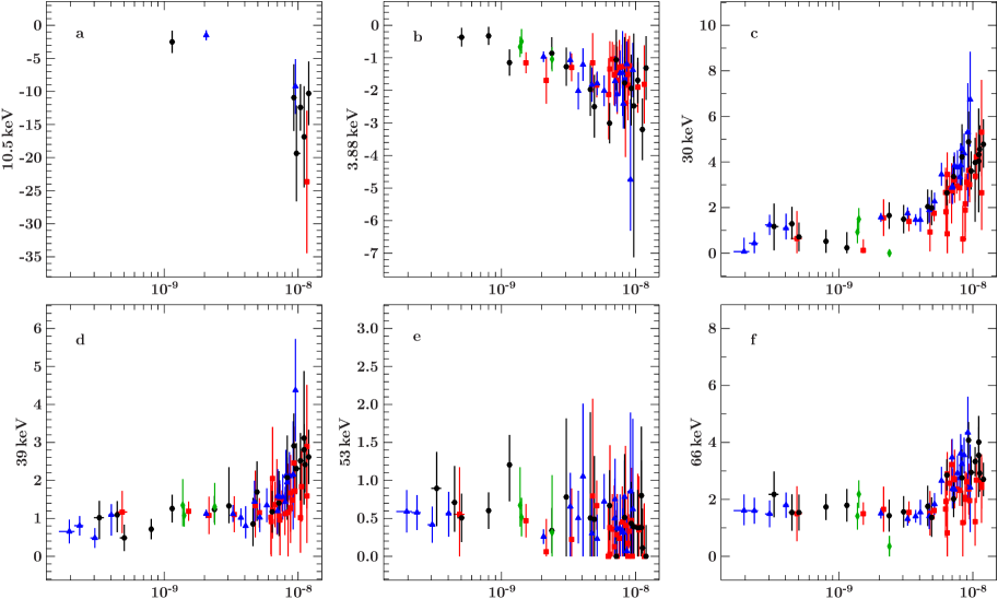
Figure 13: The various line fluxes in units of 10^-3 cm^-2 s^-1 for the highecut model plotted versus 2$-$10 keV unabsorbed flux in units of ergs cm^-2 s^-1. Data from 2010 March/April are in green, 2010 August are in black, 2010 December are in blue, and 2011 May are in red.

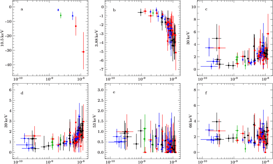
Figure 14: The various line fluxes in units of 10^-3 cm^-2 s^-1 for the cutoffpl model plotted versus 2$-$10 keV unabsorbed flux in units of ergs cm^-2 s^-1. Data from 2010 March/April are in green, 2010 August are in black, 2010 December are in blue, and 2011 May are in red.

Correlations between the fitted cyclotron line parameters and background lines at 53 keV and 66 keV, as well as versus the cutoff energy and folding energy of the continuum, are displayed in Fig. 15 and 16 for high and low flux observations #9 and #39, respectively. In addition the correlation between the folding and cutoff energies is shown for those observations.

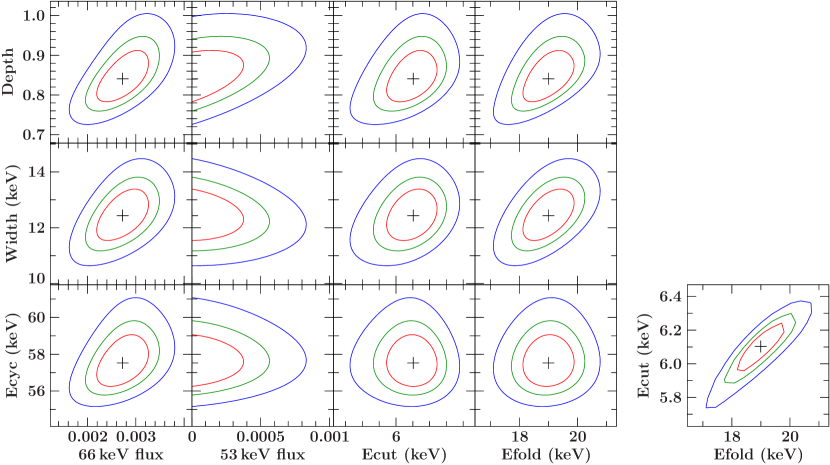
Figure 15: Contours of the cyclotron line fitted parameters versus the background lines at 66 keV, 53 keV, and the continuum parameters Ecut and Efold, plus the contours for Ecut versus Efold for observation 9. The red, green, and blue contours represent the 68%, 90%, and 99% significance levels.

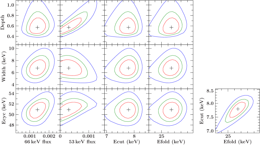
Figure 16: Contours of the cyclotron line fitted parameters versus the background lines at 66 keV, 53 keV, and the continuum parameters Ecut and Efold, plus the contours for Ecut versus Efold for observation 39. The red, green, and blue contours represent the 68%, 90%, and 99% significance levels.

Appendix C Test of HEXTE Background Estimation for GX 304$-$1

C.1 Counts and Rates

One test of the HEXTE background estimation method described above is whether or not the total number of counts in the background-subtracted HEXTE spectrum was linearly proportional to that in the background-subtracted PCU2 spectrum. Fig. 17-Left shows the product of the counting rate in the spectral band (3$-$60 keV PCU2; 20$-$100 keV HEXTE) times the lifetime per observation. The linear relationship is clearly followed with the exception of 6 observations where the HEXTE total counts are low. Since the 6 outliers are not evident in the rate plot (Fig. 17-Right), the HEXTE spectral data, from which the rates were extracted using the SHOW RATE command in XSPEC, are not suspect, and the outliers appear to be due to abnormally low lifetimes in the spectral extraction (as compared to that expected from the value of the PCU2 livetime) that resulted from missing HEXTE data. This can also be seen when one calculates the ratio of PCU2 to HEXTE livetimes.

Fig. 17-Right shows the HEXTE 20$-$100 keV counting rate versus the PCU2 3-60 keV rate. The HEXTE and PCU2 counting rates again are linearly correlated until about 500 counts/s in the PCU2. The deviation from linearity at higher rates is due to the change in the column density above a flux of $\sim 4\times 10^{-9}$ ergs cm^-2 s^-1, and the added column density during the 2011 May column density enhancement. The column density variations will affect the 3$-$60 keV PCU2 rate while leaving the 20$-$100 keV HEXTE rate unaffected.

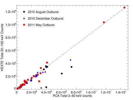
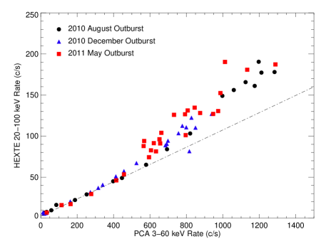
Figure 17: Left: Total PCU2 counts 3$-$60 keV versus total HEXTE-A counts 20$-$100 keV. Total counts are calculated as lifetime times count rate. The six outliers result from significantly lower HEXTE A lifetime than expected. Right: Comparison of PCU2 and HEXTE A counting rates when the HEXTE background estimation method is used. The deviations from the linear relation are due to the variation in the column depth at the higher flux levels and the column density enhancement events (see Fig. 11).

C.2 Lines and Normalizations

The various line fluxes’ variations with power law flux from the highecut and cutoffpl model fittings are shown in Figs. 13 and 14. The 10.5 keV feature (panel a) appears at the very highest fluxes in the highecut model, while being rare in the cutoffpl modeling. The 3.88 PCU2 systematic feature (panel b) shows a stronger correlation with the power law flux for the cutoffpl model than that for highecut. This could be due to the more curved shape of the cutoffpl model as compared to the straight power law in highecut. The 30 keV HEXTE background line (panel c) appears stronger at high power law flux levels in the highecut model. The other HEXTE background lines (panels d, e, & f) show similar behaviors with increasing flux in both models.

Fig. 18 gives the values of the recor parameter for PCU2 and HEXTE as well as the HEXTE constant with respect to the PCU2 flux. The top panels are for the highecut model and the bottom panels are for the cutoffpl model. In the fitting process, the corback function found in ISIS and recor function in XSPEC are used to optimize the background subtraction by adjusting the background live time as part of the fitting process. PCU2 background estimates are based upon the observed background as a function of certain instrument charged particle average counting rates, and as such, may not reflect the exact background experienced during a given observation. The spectral shape of the background is assumed to remain the same and just its intensity is adjusted via the live time. A similar estimation is done for both the effects of the averages associated with HEXTE deadtime and HEXTEBACKEST. The recor/corback free parameter is the fraction of the estimated background to be added or subtracted. , The originally determined background normalizations have to be reduced by increasing amounts for increasing source fluxes, since true X-rays can contaminate the average charged particle counting rates for sources at high fluxes in the PCU2 and HEXTE. These counting rates are the basis for the background estimates. The effect is larger in the highecut models as compared to that in the cutoffpl models.

The relative normalization between the PCU2 and HEXTE instruments is plotted in Fig. 18-Top/Bottom panel c. The HEXTE normalization constant is around 0.88 except at the lower power law fluxes where it increases with ever larger uncertainties, and at higher fluxes when the column density enhancements affect the 2$-$10 keV PCU2 fluxes.

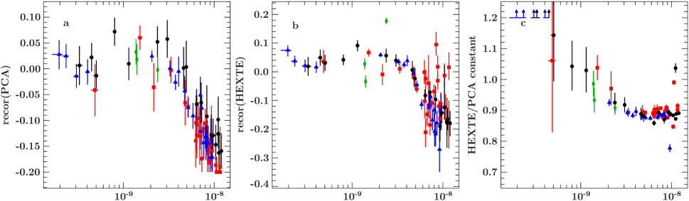
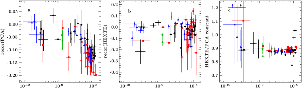
Figure 18: The variation of the recor normalization versus power law continuum flux in units of ergs cm^-2 s^-1 is shown for the PCU2 (a) and HEXTE (b), plus the relative normalization constant for the HEXTE cluster A with respect to the PCU2 normalization (c). The values resulting from highecut are plotted above those from cutoffpl.

References

- Arnaud (1996) Arnaud K.A., 1996, in Jacoby G.H. and Barnes J., eds., ASP Conf. Ser. Vol. 101, Astronomical Data Analysis Software and Systems V, Astron. Soc. Pac., San Francisco, p. 17
- Bakso & Sunyaev (1976) Basko M.M., Sunyaev R.A., 1976, MNRAS, 175, 395
- Becker et al. (2012) Becker P.T. et al., 2012, A&A, 544, A123
- Bevington & Robinson (1992) Bevington P.R., Robinson D.K.,1992, Data Reduction and Data Analysis for the Physical Sciences, McGraw-Hill, New York, 2nd Edition
- Boldin, Tsygankov & Lutovinov (2013) Boldin P.R., Tsygankov S.S., and Lutovinov A.A., 2013 AstL, 39, 375
- Bykov & Krassilshchikov (2004) Bykov A.M., Krassilshchikov A.M., 2004, Astron. Lett., 30, 309
- Caballero et al. (2008) Caballero I. et al., 2008, A&A, 480, L17
- Coburn et al. (2002) Coburn W., Heindl W.A., Rothschild R.E., Gruber D.E., Kreykenbohm I., Wilms J., Kretschmar P., Staubert R., 2002, ApJ, 580, 394
- Davidson (1973) Davidson K., 1973, Nature Physical Science, 246, 1
- Devasia et al. (2011) Devasia J., James M., Paul B., Indulekha K., 2011, MNRAS, 417, 348
- Fürst et al. (2014) Fürst F., et al. 2014, ApJ, 780, 133
- Fürst et al. (2015) Fürst, F., et al. 2015, ApJ, 806, L24
- Garasev et al. (2011) Garasev M., Derishev E., Kocharovsky V., Kocharovsky V.l., 2011, A&A, 531, L14
- Giacconi et al. (1972) Giacconi R., Murray S., Gursky H., Kellogg E., Schreier E., Tananbaum H., 1972, ApJ, 178, 281
- Houck & Denicola. (2000) Houck J.C., Denicola L.A., 2000, in Manset N., Veillet C., and Crabtree D., eds. ASP Conf. Series Vol. 216, Astronomical Data Analysis Software and Systems IX, Astron. Soc. Pac., p. 591
- Ivanov (1969) Ivanov V.V., 1969, Moskova: Nauka, 472
- Ivanov (1973) Ivanov V.V., 1973, NBS Special Publication, Washington: US Department of Commerce, National Bureau of Standards
- Jahoda et al. (2006) Jahoda K., Marquardt C.B., Radeva Y., Rots A.H., Stark M.J., Swank J.H., Strohmayer T.E., Zhang W., 2006, ApJS, 163, 401
- Jaisawal, Naik & Eplil (2016) Jaisawal G.K., Naik S., Eplil P., 2016, arXiv:16-1.02348
- Klochkov et al. (2011) Klochkov D., Staubert R., Santangelo A., Rothschild R.E., Ferrigno C., 2011, A&A, 532, A126
- Klochkov et al. (2012) Klochkov D. et al., 2012, A&A, 542, L28
- Kühnel et al. (2013) Kühnel M. et al., 2013, A&A, 555, A95
- Kühnel et al. (2016) Kühnel M. et al.,2016, in prep.
- Langer & Rappaport (1982) Langer S.H., Rappaport S., 1982, ApJ, 257, 733
- La Parola et al. (2016) La Parola V., Cusumano G., Segreto A., D’ Aì, 2016, MNRAS, 463, 185
- Lewin, Clark & Smith (1968) Lewin W.H.G., Clark G.W., Smith W.B., 1968, Nature, 219, 1235
- Lyutikov & Gavriil (2006) Lyutikov M., Gavriil F.P., 2006, MNRAS, 454, 1847
- Malacaria et al. (2015) Malacaria C., Klochkov D., Santangelo A., Staubert R., 2015, A&A, 581, A121
- Manousakis et al. (2008) Manousakis A. et al., 2008, ATEL, 1613
- Mason et al. (1978) Mason K.O., Murdin P.G., Parkes G.E., Visvanathan N., 1978, MNRAS, 184, 45P
- McClintock, Ricker & Lewin (1971) McClintock J.E., Ricker G.R., Lewin W.H.G., 1971, ApJ, 166, L63
- McClintock et al. (1977) McClintock J.E., Rappaport S.A., Nugent J.J., Li F.K.,1977, ApJ, 216, L15
- Mushtukov et al. (2015a) Mushtukov A.A., Suleimanov V.F., Tsygankov S.S., Poutanen J., 2015a, MNRAS, 447, 1847
- Mushtukov et al. (2015b) Mushtukov A.A., Tsygankov S.S., Serber A.V., Suleimanov V.F., Poutanen J., 2015b, MNRAS, 454, 2714
- Müller et al. (2013) Müller S. et al., 2015 A&A, 551, A6
- Nakajima et al. (2006) Nakajima M., Mihara T., Makishima K., Niko H., 2006, ApJ, 646, 1125
- Nelson, Salpeter & Wassermann (1993) Nelson R.W., Salpeter E.E., Wasserman I., 1993, ApJ, 418
- Nishimura (2014) Nishimura O. 2014, ApJ, 781, 30
- Parkes, Murdin & Mason (1980) Parkes G.E., Murdin P.G., Mason K.O., 1980, MNRAS, 190, 537
- Postnov et al. (2008) Postnov K., Staubert R., Santangelo A., Klochkov D., Kretschmar P., Caballero I., 2008, A&A, 480, L21
- Postnov et al. (2015a) Postnov K., Mironov A.I., Lutovinov A.A., Shakura N.I., Kochetkova A.Yu., Tsygankov S.S., 2015a, MNRAS, 446, 1013
- Postnov et al. (2015b) Postnov K.A., Gornostaev M.I., Klochkov D., Laplace E., Lukin V.V., Shakura N.I., 2015b, MNRAS, 452, 1601
- Pottschmidt et al. (2006) Pottschmidt K., Rothschild R.E., Gasaway T., Wilms J., Suchy S., Coburn, W., 2006, BAAS, 38, 384
- Poutanen et al. (2013) Poutanen J., MushTukov A.A., Suleimanov V.F., Tsygankov S.S., Nagirner D.I., Doroshenko V., Lutovinov A.A. 2013, ApJ, 777, 115
- Reig, Fabregat & Coe (1997) Reig P., Fabregat J., Coe J., 1997, A&A, 322, 193
- Reig & Nespoli (2013) Reig P., Nespoli E., 2013, A&A, 551, A1
- Rothschild et al. (1998) Rothschild R.E. et al., 1998, ApJ, 496, 538
- Shakura et al. (2012) Shakura N., Postnov K., Kochetkova A., Hjalmarsdotter L., 2012, MNRAS, 420, 216
- Shapiro & Salpeter (1975) Shapiro S.L., Salpeter E.E., 1975, ApJ, 198, 671
- Staubert et al. (2007) Staubert R., Shakura N.I., Postnov K., Wilms J., Rothschild R.E., Coburn W., Rodina L., Klochkov D., 2007 A&A, 465, L25
- Staubert et al. (2014) Staubert R., Klochkov D., Wilms J., Postnov K., Shakura, N. I., Rothschild R. E., Fürst F., Harrison F. A., 2014, A&A, 572, 119
- Staubert et al. (2016) Staubert R., Klochkov D., Vyobornov V., Wilms J., Harrison F., 2016, A&A, in print
- Sugizaki et al. (2015) Sugizaki M., Yamamoto T., Mihara T., Nakajima M., Makishima K., 2015, PASJ, 67, 73
- Trümper et al. (1978) Trümper J., Pietsch W., Reppin C., Voges W., Staubert R., Kendziorra E., 1978, ApJ, Lett. 219, L105
- Tsygankov et al. (2006) Tsygankov S.S., Lutovinov A.A., Churazov E.M., Sunyaev R.A., 2006, MNRAS, 371, 19
- Verner & Yakovlev (1995) Verner D.A., Yakovlev D.G., 1995, A&AS, 109, 125
- Wasserman & Saltpeter (1980) Wasserman I., Saltpeter E., 1980, ApJ, 241, 1107
- Wilms, Allen & McCray (2000) Wilms J., Allen A., McCray R., 2000, ApJ, 542, 914
- Yamamoto et al. (2011) Yamamoto, T. et al., 2011, PASJ, 63, S751
- Zheleznyakov (1996) Zheleznyakov V., 1996, Radiation in Astrophysical Plasmas, Astrophysics & Space Science Library vol. 204