Lifetime and mass of rho meson in correlation with
magnetic-dimensional reduction

Abstract

It is simply anticipated that in a strong magnetic configuration, the Landau quantization ceases the neutral rho meson to decay to the charged pion pair, so the neutral rho meson will be long-lived. To closely access this naive observation, we explicitly compute the charged pion-loop in the magnetic field at the one-loop level, to evaluate the magnetic dependence of the lifetime for the neutral rho meson as well as its mass. Due to the dimensional reduction induced by the magnetic field (violation of the Lorentz invariance), the polarization (spin $s_{z}=0,\pm 1$) modes of the rho meson, as well as the corresponding pole mass and width, are decomposed in a nontrivial manner compared to the vacuum case. To see the significance of the reduction effect, we simply take the lowest-Landau level approximation to analyze the spin-dependent rho masses and widths. We find that the “fate” of the rho meson may be more complicated because of the magnetic-dimensional reduction: as the magnetic field increases, the rho width for the spin $s_{z}=0$ starts to develop, reach a peak, to be vanishing at the critical magnetic field to which the folklore refers. On the other side, the decay rates of the other rhos for $s_{z}=\pm 1$ monotonically increase as the magnetic field develops. The correlation between the polarization dependence and the Landau-level truncation is also addressed.

I Introduction

Studies on hadron properties under the influence of the magnetic field have been extensively done so far. The development on such a hadron physics in the magnetic field would be relevant to gain some new insights for existing environment systems with the presence of strong magnetic fields, like in relativistic heavy ion collision Kharzeev:2007jp ; Skokov:2009qp and neutron stars Harding:2006qn ; Lattimer:2006xb ; Potekhin:2011xe ; Lai:2014nma .

In the magnetic field, hadron properties will indeed be dramatically changed. For the neutral rho meson, in particular, it is expected that the decay channel to the charged pion pair, which is the main decay mode in the vacuum (without the magnetic configuration), will be closed, and hence the neutral rho meson can be long-lived. This is a naively-believed folklore, which can be reasoned by the Landau quantization for the charged pions: in the vacuum the neutral rho-meson decay width to the charged pion pair, $\Gamma(\rho\to\pi\pi)$, is given as

$$\Gamma(\rho^{0}\to\pi^{+}\pi^{-})_{\rm vac}=\frac{|g_{\rho\pi\pi}|^{2}}{6\pi m_{\rho}^{2}}\left(\sqrt{\frac{m_{\rho}^{2}-4m_{\pi}^{2}}{4}}\right)^{3}\,,$$ (I.1)

with the $\rho^{0}-\pi^{+}-\pi^{-}$ coupling strength $g_{\rho\pi\pi}(\simeq 6)$. Now, turn on the magnetic field. Since the charged pions carry the electromagnetic charge, the mass ($m_{\pi}$) will be shifted by the magnetic field to be $\sqrt{m_{\pi}^{2}+eB}$ in the lowest Landau level (LLL). Then, one may naively suspect that the decay width in Eq.(I.1) will be modified in the phase space factor like

$$\Gamma(\rho^{0}\to\pi^{+}\pi^{-})_{\rm naive}=\frac{|g_{\rho\pi\pi}|^{2}}{6\pi m_{\rho}^{2}}\left(\sqrt{\frac{m_{\rho}^{2}-4(m_{\pi}^{2}+eB)}{4}}\right)^{3}\,.$$ (I.2)

Thus, the $\rho^{0}\to\pi^{+}\pi^{-}$ decay channel is expected to be closed when the magnetic field reaches the critical scale $eB_{c}=(m_{\rho}^{2}-4m_{\pi}^{2})/4\simeq 0.13\,{\rm GeV}^{2}$.

Note that the above widely-accepted argument invokes only the kinematics, relying on the modification of the phase space factor: the dynamical properties in the magnetic field, such as the dimensional reduction, are not taken into account at all. Therefore, a more rigorous argument on this issue should involve some explicit dynamical computation of the rho width.

In this paper, we explicitly compute the charged pion-loop in the magnetic field at the one-loop level based on a chiral effective model. We evaluate the magnetic dependence of the decay width (lifetime) for the neutral rho meson as well as its mass. We find that the polarization (spin $s_{z}=0,\pm 1$) modes of the rho meson, as well as the corresponding pole mass and width, are decomposed in a nontrivial manner compared to the vacuum case. This is due to the dimensional reduction induced by the magnetic field.

In order to study the significance of the reduction effect, we simply take the LLL approximation and analyze the spin-dependent rho masses and widths. We find that as the magnetic field increases, the rho width for the spin $s_{z}=0$ starts to develop, reach a peak, to be vanishing at the critical magnetic field to which the folklore refers: this result would suggest that the “fate” of the neutral rho meson in the magnetic field may be more complicated than the aforementioned naive expectation. On the other side, the decay rates of the other rhos for $s_{z}=\pm 1$ monotonically increase as the magnetic field develops. The correlation between the polarization dependence and the Landau-level truncation is also addressed.

This paper is constructed as follows: in Sec. II we introduce a chiral-effective model and extract the Lagrangian terms relevant to the later discussions. Sec. III provides the explicit computation of the pion-loop contribution, including the effect of the magnetic-dimensional reduction, to the rho meson propagator at the one-loop level. In Sec. IV we numerically evaluate the magnetic dependence of the neutral rho meson with respect to the polarization states intrinsically decomposed by the presence of the magnetic field. Some possible interpretations for the results obtained in Sec. IV are proposed in Sec. V. Summary is given in Sec. VI. The appendix A provides formulae for the Feynman parameter integrals relevant to evaluation of the one-loop terms given in Sec. III.

II A chiral effective model

We employ a chiral effective model based on the coset space, $G/H=[SU(2)_{L}\times SU(2)_{R}\times U(1)_{V}]/SU(2)_{V=L=R}\times U(1)_{V}$. The fundamental dynamical variables to construct the chiral effective Lagrangian are the nonlinear bases $\xi_{L,R}$, which transform under the $G$ as $\xi_{L,R}\rightarrow h(\pi,g_{L},g_{R})\cdot\xi_{L,R}\cdot g^{\dagger}_{L,R}$, where $h(\pi,g_{L},g_{R})\in H$ and $g_{L,R}\in G$. These variables are parameterized by the pions as $\xi_{L,R}=e^{\mp i\pi^{a}T^{a}/F_{\pi}}$ with $\pi^{a}$ $(a=1,2,3)$ being the pion fields, $T^{a}$ generators of $SU(2)$ normalized by ${\rm tr}[T^{a}T^{b}]=\delta^{ab}/2$ and $F_{\pi}$ is the pion decay constant. It is convenient to introduce the Maurer-Cartan 1-forms:

$$\alpha_{\perp,||\mu}=\frac{1}{2i}(D_{\mu}\xi_{R}\cdot\xi^{\dagger}_{R}\mp D_{\mu}\xi_{L}\cdot\xi^{\dagger}_{L})\,.$$ (II.3)

Here we have gauged the chiral symmetry with the external gauge fields ${\cal L}_{\mu}$ and ${\cal R}_{\mu}$, and

$$D_{\mu}\xi_{L} = \partial_{\mu}\xi_{L}+i\xi_{L}{\cal L}_{\mu}\,,$$

$$D_{\mu}\xi_{R} = \partial_{\mu}\xi_{R}+i\xi_{R}{\cal R}_{\mu}\,,$$ (II.4)

with the photon field $A_{\mu}$ incorporated as ${\cal L}_{\mu}={\cal R}_{\mu}=eQ_{\rm em}A_{\mu}$ involving the electromagnetic coupling $e$ and the charge matrix $Q_{\rm em}=T^{3}+1/6\cdot{\bm{1}}_{2\times 2}={\rm diag}(2/3,-1/3)$. The 1-forms $\alpha_{\perp,||\mu}$ transform under the $G$ as

$$\alpha_{\perp\mu} \rightarrow h(\pi,g_{L},g_{R})\cdot\alpha_{\perp\mu}\cdot h^{\dagger}(\pi,g_{L},g_{R})\,,$$

$$\alpha_{||\mu} \rightarrow h(\pi,g_{L},g_{R})\cdot\alpha_{||\mu}\cdot h^{\dagger}(\pi,g_{L},g_{R})-i\partial_{\mu}h(\pi,g_{L},g_{R})\cdot h^{\dagger}(\pi,g_{L},g_{R}).$$ (II.5)

We include the vector meson field as a matter field (a la Callan-Coleman-Wess-Zumino) in the adjoint representation, $\rho_{\mu}=\rho_{\mu}^{a}T_{a}$, which transforms homogeneously under the chiral symmetry as $\rho_{\mu}\rightarrow h(\pi,g_{R},g_{L})\cdot\rho_{\mu}\cdot h^{\dagger}(\pi,g_{L},g_{R})$. The chiral-covariant derivative for the $\rho_{\mu}$ is then defined by $D_{\mu}\rho_{\nu}=\partial_{\mu}\rho_{\nu}-i[\alpha_{||\mu},\rho_{\nu}]$. The chiral invariant Lagrangian including the $\rho$ meson and the $\pi$ meson is thus written as

$${\cal L} = F_{\pi}^{2}{\rm tr}[\alpha_{\perp\mu}\alpha^{\mu}_{\perp}]+\frac{F_{\pi}^{2}}{4}{\rm tr}[\hat{\chi}^{\dagger}+\hat{\chi}]$$ (II.6)

$$-\frac{1}{2}{\rm tr}[\rho_{\mu\nu}\rho^{\mu\nu}]+m_{\rho}^{2}{\rm tr}[\rho_{\mu}\rho^{\mu}]-i{\cal G}{\rm tr}[\rho_{\mu\nu}\alpha_{\perp}^{\mu}\alpha_{\perp}^{\nu}],$$

where $\rho_{\mu\nu}=D_{\mu}\rho_{\nu}-D_{\nu}\rho_{\mu}$ and ${\cal G}$ is a coupling constant related to the $\rho-\pi-\pi$ vertex. In Eq.(II.6) we also introduced the pion mass term (the second term in the first line) in which the chiral invariance is ensured by the spurion field $\hat{\chi}=\xi_{L}\chi\xi_{R}^{\dagger}$ having the transformation law $\chi\to g_{L}\cdot\chi\cdot g^{\dagger}_{R}$. When the $\chi$ gets the vacuum expectation value, $\langle\chi\rangle=m_{\pi}^{2}\cdot{\bm{1}}_{2\times 2}$, the second term gives the pion mass.

Expanding the 1-forms in Eq.(II.3) in powers of the pion field, we extract portions relevant to the present study,

$${\cal L}_{\rho^{0},\pi^{\pm}} = D_{\mu}\pi^{+}D^{\mu}\pi^{-}-m_{\pi}^{2}\pi^{+}\pi^{-}-\frac{1}{2}(\partial_{\mu}\rho^{0}_{\nu}-\partial_{\nu}\rho^{0}_{\mu})(\partial^{\mu}\rho^{0\nu}-\partial^{\nu}\rho^{0\mu})+\frac{1}{2}m_{\rho}^{2}\rho^{0}_{\mu}\rho^{0\mu}$$ (II.7)

$$+ig_{\rho\pi\pi}\rho^{0\mu}(\partial_{\mu}\pi^{+}\cdot\pi^{-}-\partial_{\mu}\pi^{-}\cdot\pi^{+}),$$

where we defined $D_{\mu}\pi^{\pm}=(\partial_{\mu}\mp ieA_{\mu})\pi^{\pm}$ for the charged pions, $\pi^{\pm}\equiv(\pi^{1}\mp i\pi^{2})/\sqrt{2}$, and used the equation of motion for the rho field to get the on-shell $\rho-\pi-\pi$ coupling, $g_{\rho\pi\pi}={\cal G}m_{\rho}^{2}/(4F_{\pi}^{2})$ in the last line, which is experimentally $\simeq 6$ in the vacuum. The covariantized-pion kinetic term ($|D_{\mu}\pi^{\pm}|^{2}$) in Eq.(II.7) provides the charged-pion propagator under the magnetic field $B$ (in $A_{\mu}$). It can be expressed by the Schwinger’s proper-time procedure Schwinger:1951nm . In the present analysis, instead of the Schwinger form, we shall take a form expanded in terms of the Landau levels as done in Ref. Ayala:2004dx .

Let us consider the constant magnetic field $B$ oriented along the $z$-direction in the position-space time. The $\pi^{\pm}$ propagator, $G^{B}(x,y)$, then takes the form

$$G^{B}(x,y)=\Phi(x,y)\int\frac{d^{4}p}{(2\pi)^{4}}G^{B}(p)e^{-ip\cdot(x-y)}\,,$$ (II.8)

where

$$\Phi(x,y) = \exp\left[ie\int_{y}^{x}dx^{\prime}_{\mu}A^{\mu}(x^{\prime})\right]\,,$$

$$G^{B}(p) = 2i\sum_{l=0}^{\infty}(-1)^{l}L_{l}\left(2\frac{p_{\perp}^{2}}{eB}\right)\exp\left[\frac{p_{\perp}^{2}}{eB}\right]\frac{1}{p_{||}^{2}-(2l+1)eB-m^{2}_{\pi}}\,,$$ (II.9)

with $L_{l}\left(2\frac{p_{\perp}^{2}}{eB}\right)$ being the Laguerre polynomials labeling the Landau level as $l$. In Eq.(II.9) we have introduced the following notations for the four-momenta:

$$p_{||}^{\mu}=(p^{t},0,0,p^{z}),\,\,\,\,\,p_{\perp}^{\mu}=(0,p^{x},p^{y},0)\,,$$

$$p_{||}^{2}=(p^{t})^{2}-(p^{z})^{2},\,\,\,p_{\perp}^{2}=-(p^{x})^{2}-(p^{y})^{2}\,.$$ (II.10)

Note also that the functional $\Phi(x,y)$ obviously depends on the gauge. Here we shall choose the gauge so as to set $\Phi\equiv 1$.

From the propagator expression in Eq.(II.9), one should note that since nonzero constant magnetic field is present, no matter how small it is, the Lorentz invariance in four-dimension has been lost: the propagation of the $\pi^{\pm}$ is now confined to the z-direction parallel to the magnetic field. This is the consequence of the dimensional reduction.

III rho meson propagator on the magnetic-dimensional reduction

In this section, based on the Lagrangian Eq.(II.7) and the $\pi^{\pm}$ propagator $G^{B}$ in Eq.(II.9) (with $\Phi=1$), we shall compute and evaluate the $\pi^{\pm}$-loop corrections to the $\rho^{0}$ propagator at the one-loop level. As noted in the last paragraph of Sec. II, due to the magnetic-dimensional reduction the $\rho^{0}$ propagator and polarization structure no longer take the Lorentz-covariant form. To see the effect of the significant reduction, we shall hereafter take the LLL approximation and explicitly evaluate how the effect of the magnetic-dimensional reduction for the $\pi^{\pm}$ propagator is transferred to the $\rho^{0}$-polarization structure, mass and widths.

By including the one-loop correction arising from the $\rho-\pi-\pi$ vertex with the coupling strength in Eq.(II.7), the resultant inversed-$\rho^{0}$ propagator is expressed as

$$D^{-1}_{\mu\nu}=D^{-1}_{F\mu\nu}+\Pi_{\mu\nu},$$ (III.11)

where $D^{-1}_{F\mu\nu}(p)=-(p^{2}-m^{2}_{\rho})g_{\mu\nu}+p_{\mu}p_{\nu}$ denotes the free inversed-propagator and $\Pi_{\mu\nu}$ is the self-energy function,

$$i\Pi_{\mu\nu}=-4(g_{\rho\pi\pi})^{2}\int\frac{d^{4}k}{(2\pi)^{4}}k_{\mu}k_{\nu}G^{B}(k-\frac{p}{2})G^{B}(k+\frac{p}{2})\,.$$ (III.12)

In the LLL approximation (with only $l=0$ kept in Eq.(II.9)), the $\Pi_{\mu\nu}$ is decomposed by reflecting the dimensional reduction:

$$i\Pi_{\mu\nu}(p_{||}^{2},p_{\perp}^{2})=i\left(\Pi_{||}^{S}(p^{2}_{||},p_{\perp}^{2})g_{||\mu\nu}+\Pi_{||}^{T}(p^{2}_{||},p_{\perp}^{2})(p_{||}^{2}g_{||\mu\nu}-p_{||\mu}p_{||\nu})+\Pi_{\perp}^{S}(p^{2}_{||},p_{\perp}^{2})g_{\perp\mu\nu}\right)\,,$$ (III.13)

where $g_{||\mu\nu}={\rm diag}(1,0,0-1)$ and $g_{\perp\mu\nu}={\rm diag}(0,-1,-1,0)$, and

$$\Pi_{||}^{S}(p_{||}^{2},p_{\perp}^{2}) = \frac{2(eB)}{(4\pi)^{2}}(g_{\rho\pi\pi})^{2}e^{\frac{p_{\perp}^{2}}{2eB}}\int_{0}^{1}dx\Bigl{(}-2\ln\frac{\Lambda^{2}}{\Delta}+p_{||}^{2}(2x-1)^{2}\frac{1}{\Delta}\Bigl{)}\,,$$

$$\Pi_{||}^{T}(p_{||}^{2},p_{\perp}^{2}) = -\frac{2(eB)}{(4\pi)^{2}}(g_{\rho\pi\pi})^{2}e^{\frac{p_{\perp}^{2}}{2eB}}\int_{0}^{1}dx\frac{(2x-1)^{2}}{\Delta}\,,$$

$$\Pi_{\perp}^{S}(p_{||}^{2},p_{\perp}^{2}) = -\frac{2(eB)}{(4\pi)^{2}}(g_{\rho\pi\pi})^{2}e^{\frac{p_{\perp}^{2}}{2eB}}\int_{0}^{1}dx\frac{eB}{\Delta}\,,$$ (III.14)

with $\Delta=x(x-1)p_{||}^{2}+m_{\pi}^{2}+eB$. (The relevant formulas for the Feynman parameter integrals in Eq.(III.14) are presented in Appendix A.) In evaluating the loop integrals, one has encountered the divergent term, which has been regularized by the dimensional regularization with the $D=2$ pole being replaced by the cutoff dependence $\Lambda$. Note that the overall factors of $(eB)$ in Eq.(III.14) come from the loop integrations of the pion momentum along the perpendicular direction ($k_{\perp}$ in Eq.(III.12)). That is the consequence of the dimensional reduction.

By performing the inversion of Eq.(III.11), one finds the propagator $D_{\mu\nu}$ in the presence of the magnetic field $(F_{\mu\nu}=\partial_{\mu}A_{\nu}-\partial_{\nu}A_{\mu}=B(\delta_{\mu 1}\delta_{\nu 2}-\delta_{\nu 1}\delta_{\mu 2})$), which can generically be decomposed into four independent polarization structures Ritus:1972ky ; Shabad:1975ik ; Hattori:2012je :

$$D_{\mu\nu}=D_{p}\frac{p_{\mu}p_{\nu}}{p^{2}}+D_{L}\frac{L_{\mu}L_{\nu}}{L^{2}}+D_{Q}\frac{Q^{*}_{\mu}Q_{\nu}}{Q^{*}\cdot Q}+D_{G}\frac{G_{\mu}G_{\nu}}{G^{2}}\,,$$ (III.15)

where the polarization vectors $L_{\mu},Q_{\mu}$ and $G_{\mu}$ are defined as

$$L^{\mu}=F^{\mu\nu}p_{\nu}=-B(0,p^{y},-p^{x},0)\,,$$

$$Q^{\mu}=\frac{i}{2}\epsilon^{\mu\nu\rho\sigma}F_{\rho\sigma}p_{\nu}=iB(-p^{z},0,0,-p^{t})\,,$$

$$G^{\mu}=(p^{2}/L_{\mu}L^{\mu})F^{\mu\nu}F_{\nu\lambda}p^{\lambda}+p^{\mu}=\left(p^{t},-\frac{p_{||}^{2}}{p_{\perp}^{2}}p^{x},-\frac{p_{||}^{2}}{p_{\perp}^{2}}p^{y},p^{z}\right)\,,$$ (III.16)

and

$$D_{p} = \frac{i}{m_{\rho}^{2}+\Pi_{||}^{S}\frac{p^{2}_{||}}{p^{2}}+\Pi_{\perp}^{S}\frac{p^{2}_{\perp}}{p^{2}}}\,,$$

$$D_{L} = \frac{i}{m_{\rho}^{2}-p^{2}+\Pi_{\perp}^{S}}\,,$$

$$D_{Q} = \frac{i}{m_{\rho}^{2}-p^{2}+\Pi_{||}^{S}+p^{2}_{||}\Pi_{||}^{T}}\,,$$

$$D_{G} = \frac{i}{m_{\rho}^{2}-p^{2}+\Pi^{S}_{||}\frac{p_{\perp}^{2}}{p^{2}}+\Pi_{\perp}^{S}\frac{p^{2}_{||}}{p^{2}}}\,.$$ (III.17)

It turns out that the polarization mode along with the $D_{p}$ corresponds to the unphysical degree of freedom, like a scalar mode. (One can easily check it by constructing the equation of motion corresponding to the $D_{p}$ propagator form and finding that it satisfies the Klein-Gordon equation, so it is nothing but a scalar with spin $S=0$.) For the other three physical modes, $L_{\mu},Q_{\mu}$ and $G_{\mu}$, the $\rho^{0}$ effective masses are defined as

$$M_{L}^{2} = m_{\rho}^{2}+{\rm Re}\,\Pi_{\perp}^{S}(p^{t}=M_{L},\vec{p}=\vec{0})\,,$$

$$M_{Q}^{2} = m_{\rho}^{2}+{\rm Re}\,\Pi_{||}^{S}(p^{t}=M_{Q},\vec{p}=\vec{0})+M_{Q}^{2}{\rm Re}\,\Pi_{||}^{T}(p^{t}=M_{Q},\vec{p}=\vec{0})\,,$$

$$M_{G}^{2} = m_{\rho}^{2}+{\rm Re}\,\Pi_{\perp}^{S}(p^{t}=M_{G},\vec{p}=\vec{0})\,,$$ (III.18)

where $\vec{p}=(p^{x},p^{y},p^{z})$. To be canonical, the neutral $\rho^{(L)}$, $\rho^{(Q)}$ and $\rho^{(G)}$ fields are rescaled by the field renormalization constants $Z_{L}$, $Z_{Q}$ and $Z_{G}$ respectively:

$$Z_{L}^{-1} = 1-\frac{\partial{\rm Re}\,\Pi_{\perp}^{S}(p^{2}_{||},p_{\perp}^{2})}{\partial p^{2}_{||}}\Biggl{|}_{p^{t}=M_{L},{\vec{p}}=\vec{0}}\,,$$

$$Z_{Q}^{-1} = 1-\frac{\partial\left({\rm Re}\,\Pi_{||}^{S}(p^{2}_{||},p_{\perp}^{2})+p^{2}_{||}{\rm Re}\,\Pi_{||}^{T}(p^{2}_{||},p_{\perp}^{2})\right)}{\partial p^{2}_{||}}\Bigl{|}_{p^{t}=M_{Q},{\vec{p}}=\vec{0}}\,,$$

$$Z_{G}^{-1} = 1-\frac{\partial{\rm Re}\,\Pi_{\perp}^{S}(p^{2}_{||},p_{\perp}^{2})}{\partial p_{||}^{2}}\Biggl{|}_{p^{t}=M_{G},{\vec{p}}=\vec{0}}\,.$$ (III.19)

By expanding the propagators around the effective masses of $\rho^{(L)}$, $\rho^{(Q)}$ and $\rho^{(G)}$ fields, the functions $D_{L},D_{Q}$ and $D_{G}$ in Eq.(III.17) take the forms

$$D_{L} = \frac{-iZ_{L}}{p^{2}_{||}-M_{L}^{2}+Z_{L}\left(1-\frac{\partial{\rm Re}\,\Pi_{\perp}^{S}}{\partial p^{2}_{\perp}}\Bigl{|}_{p^{t}=M_{L},\vec{p}=\vec{0}}\right)p^{2}_{\perp}-iZ_{L}{\rm Im}\,\Pi_{\perp}^{S}}+\cdots\,,$$

$$D_{Q} = \frac{-iZ_{Q}}{p^{2}_{||}-M_{Q}^{2}+Z_{Q}\left(1-\frac{\partial\bigl{(}{\rm Re}\,\Pi_{||}^{S}+p^{2}_{||}{\rm Re}\,\Pi_{||}^{T}\bigl{)}}{\partial p^{2}_{\perp}}\Bigl{|}_{p^{t}=M_{Q},\vec{p}=\vec{0}}\right)p^{2}_{\perp}-iZ_{Q}{\rm Im}\,\Pi_{||}^{S}-iZ_{Q}{\rm Im}\,\Pi_{||}^{T}\cdot p^{2}_{||}}+\cdots\,,$$

$$D_{G} = \frac{-iZ_{G}}{p^{2}_{||}-M_{G}^{2}+Z_{G}\left(1-\frac{\partial\bigl{(}\frac{p_{\perp}^{2}}{p^{2}}\Pi^{S}_{||}+\frac{p_{||}^{2}}{p^{2}}\Pi_{\perp}^{S}\bigl{)}}{\partial p^{2}_{\perp}}\Bigl{|}_{p^{t}=M_{G},\vec{p}=\vec{0}}\right)p^{2}_{\perp}-iZ_{G}{\rm Im}\,\Pi^{S}_{||}\cdot\frac{p_{\perp}^{2}}{p^{2}}-iZ_{G}{\rm Im}\,\Pi_{\perp}^{S}\cdot\frac{p_{||}^{2}}{p^{2}}}+\cdots\,,$$ (III.20)

where the ellipses denote terms having no pole structure.

As to the decay width to the LLL-charged pions ($\pi^{\pm}_{(l=0)}$), we assume the Breit-Wigner form for the propagators to extract the imaginary parts in Eq.(III.20):

$$\Gamma(\rho^{(L)}\to\pi^{+}_{(l=0)}\pi^{-}_{(l=0)}) = -\frac{Z_{L}{\rm Im}\,\Pi^{S}_{\perp}(M_{L},\vec{0})}{M_{L}}\,,$$

$$\Gamma(\rho^{(Q)}\to\pi^{+}_{(l=0)}\pi^{-}_{(l=0)}) = -Z_{Q}\frac{{\rm Im}\,\Pi_{||}^{S}(M_{Q},\vec{0})+M^{2}_{Q}{\rm Im}\,\Pi_{||}^{T}(M_{Q},\vec{0})}{M_{Q}}\,,$$

$$\Gamma(\rho^{(G)}\to\pi^{+}_{(l=0)}\pi^{-}_{(l=0)}) = -\frac{Z_{G}{\rm Im}\,\Pi_{\perp}^{S}(M_{G},\vec{0})}{M_{G}}\,.$$ (III.21)

Note from Eqs.(III.18) and (III.19) that the mass and the decay width for the $\rho^{(L)}$ coincide with those of the $\rho^{(G)}$.

IV The magnetic dependence of masses and widths

In the previous section we derived the formulae for masses and widths at the one-loop level of the chiral effective model, which have been decomposed into the intrinsic polarization modes ($\rho^{(L)},\rho^{(Q)},\rho^{(G)}$) by the magnetic-dimensional reduction. Thus we are now ready to numerically study the magnetic dependence of the rho meson masses and widths.

First of all, to be fully consistent with the one-loop level computation, we expand the formulae of masses and widths in Eqs.(III.18) and (III.21), with the Feynman parameter integrals in Eq.(III.14) properly evaluated, up to terms of order of ${\cal O}((g_{\rho\pi\pi}/4\pi)^{2})$, to get

$$M_{L/G}^{2} = \begin{cases}m_{\rho}^{2}+8(eB)^{2}\left(\frac{g_{\rho\pi\pi}}{4\pi}\right)^{2}\frac{1}{m_{\rho}\sqrt{m_{\rho}^{2}-4(m_{\pi}^{2}+eB)}}\ln\frac{\sqrt{m_{\rho}^{2}-4(m_{\pi}^{2}+eB)}+m_{\rho}}{2\sqrt{m_{\pi}^{2}+eB}}\\ \,\,\,\,\,\,\,\,\,\,\,\,\,\,\,\,\,\,\,\,\,\,\,\,\,\,\,\,\,\,\,\,\,\,\,\,\,\,\,\,\,\,\,\,\,\,\,\,\,\,\,\,\,\,\,\,\,\,\,\,\,\,\,\,\,\,\,\,\,\,\,\,\,\,\,\,\,\,\,\,\,\,\,\,\,\,\,\,\,\,\,\,\,\,\,\,\,\,\,\,\,\,\,\,\,\,\,\,\,\,\,\,\,\,\,\,\,\,\,\,\,\,\,\,\,\,\,\,\,\,\,\,\,\,\,({\rm for}\,\,\,\,\,eB<\frac{m_{\rho}^{2}-4m_{\pi}^{2}}{4})\\ m_{\rho}^{2}-8(eB)^{2}\left(\frac{g_{\rho\pi\pi}}{4\pi}\right)^{2}\frac{1}{m_{\rho}\sqrt{4(m^{2}_{\pi}+eB)-m_{\rho}^{2}}}\arctan\left(\frac{m_{\rho}}{\sqrt{4(m^{2}_{\pi}+eB)-m_{\rho}^{2}}}\right)\\ \,\,\,\,\,\,\,\,\,\,\,\,\,\,\,\,\,\,\,\,\,\,\,\,\,\,\,\,\,\,\,\,\,\,\,\,\,\,\,\,\,\,\,\,\,\,\,\,\,\,\,\,\,\,\,\,\,\,\,\,\,\,\,\,\,\,\,\,\,\,\,\,\,\,\,\,\,\,\,\,\,\,\,\,\,\,\,\,\,\,\,\,\,\,\,\,\,\,\,\,\,\,\,\,\,\,\,\,\,\,\,\,\,\,\,\,\,\,\,\,\,\,\,\,\,\,\,\,\,\,\,\,\,\,\,({\rm for}\,\,\,\,\,\frac{m_{\rho}^{2}-4m_{\pi}^{2}}{4}<eB)\,,\end{cases}$$

$$M^{2}_{Q} = \begin{cases}m_{\rho}^{2}-4(eB)\left(\frac{g_{\rho\pi\pi}}{4\pi}\right)^{2}\Biggl{(}\ln\frac{\Lambda^{2}}{m^{2}_{\pi}+eB}+2-\frac{2}{m_{\rho}}\sqrt{m_{\rho}^{2}-4(m^{2}_{\pi}+eB)}\ln\frac{\sqrt{m_{\rho}^{2}-4(m^{2}_{\pi}+eB)}+m_{\rho}}{2\sqrt{m_{\pi}^{2}+eB}}\Biggl{)}\\ \,\,\,\,\,\,\,\,\,\,\,\,\,\,\,\,\,\,\,\,\,\,\,\,\,\,\,\,\,\,\,\,\,\,\,\,\,\,\,\,\,\,\,\,\,\,\,\,\,\,\,\,\,\,\,\,\,\,\,\,\,\,\,\,\,\,\,\,\,\,\,\,\,\,\,\,\,\,\,\,\,\,\,\,\,\,\,\,\,\,\,\,\,\,\,\,\,\,\,\,\,\,\,\,\,\,\,\,\,\,\,\,\,\,\,\,\,\,\,\,\,\,\,\,\,\,\,\,\,\,\,\,\,\,\,({\rm for}\,\,\,\,\,eB<\frac{m_{\rho}^{2}-4m_{\pi}^{2}}{4})\\ m_{\rho}^{2}-4(eB)\left(\frac{g_{\rho\pi\pi}}{4\pi}\right)^{2}\Biggl{(}\ln\frac{\Lambda^{2}}{m^{2}_{\pi}+eB}+2-\frac{2}{m_{\rho}}\sqrt{4(m^{2}_{\pi}+eB)-m_{\rho}^{2}}\arctan\frac{m_{\rho}}{\sqrt{4(m^{2}_{\pi}+eB)-m_{\rho}^{2}}}\Biggl{)}\\ \,\,\,\,\,\,\,\,\,\,\,\,\,\,\,\,\,\,\,\,\,\,\,\,\,\,\,\,\,\,\,\,\,\,\,\,\,\,\,\,\,\,\,\,\,\,\,\,\,\,\,\,\,\,\,\,\,\,\,\,\,\,\,\,\,\,\,\,\,\,\,\,\,\,\,\,\,\,\,\,\,\,\,\,\,\,\,\,\,\,\,\,\,\,\,\,\,\,\,\,\,\,\,\,\,\,\,\,\,\,\,\,\,\,\,\,\,\,\,\,\,\,\,\,\,\,\,\,\,\,\,\,\,\,\,({\rm for}\,\,\,\,\,\frac{m_{\rho}^{2}-4m_{\pi}^{2}}{4}<eB)\,,\end{cases}$$

and

$$\Gamma(\rho^{(L/G)}\to\pi^{+}_{(l=0)}\pi^{-}_{(l=0)}) = \frac{(eB)^{2}(g_{\rho\pi\pi})^{2}}{8\pi m_{\rho}^{2}}\sqrt{\frac{4}{m_{\rho}^{2}-4(m_{\pi}^{2}+eB)}}\,\,\,\,\,\,\,\,\,({\rm for}\,\,\,\,\,eB<\frac{m_{\rho}^{2}-4m_{\pi}^{2}}{4})\,,$$

$$\Gamma(\rho^{(Q)}\to\pi^{+}_{(l=0)}\pi^{-}_{(l=0)}) = \frac{eB(g_{\rho\pi\pi})^{2}}{\pi m_{\rho}^{2}}\sqrt{\frac{m_{\rho}^{2}-4(m_{\pi}^{2}+eB)}{4}}\,\,\,\,\,\,\,({\rm for}\,\,\,\,\,eB<\frac{m_{\rho}^{2}-4m_{\pi}^{2}}{4}).$$ (IV.23)

Here one should also notice from Eq.(LABEL:effmass) that the consistency of the one-loop computation including the constant magnetic scale requires the $eB$ to be constrained in such a way that the one-loop terms in total should be smaller than the vacuum term $(m_{\rho}^{2})$. Thus the magnetic scale is bounded from above as

$$eB\ll\frac{4\pi m_{\rho}^{2}}{g_{\rho\pi\pi}}\sim 1\,{\rm GeV}^{2}\,.$$ (IV.24)

Furthermore, since our computation has been restricted only to the LLL approximation, the magnetic scale $eB$ actually has the lower bound: it is set by requiring the $(eB)$ not to exceed the scale above which the decay channel involving at least one pion labeled as the the next-to-LLL is open, namely,

$$\Bigl{(}\sqrt{m_{\pi}^{2}+eB}+\sqrt{m_{\pi}^{2}+3eB}\Bigl{)}^{2}>m_{\rho}^{2}\,,$$ (IV.25)

where the $(m_{\pi}^{2}+1(3)eB)$ correspond to the LLL (the next-to-LLL) pion mass.

In Fig. 1 we plot the masses in Eq.(LABEL:effmass) and the decay widths in Eq.(IV.23) as a function of the magnetic scale $(eB)$. We have used the experimental values in the vacuum Agashe:2014kda , $m_{\pi^{\pm}}=0.140\,{\rm GeV}$, $m_{\rho}=0.775\,{\rm GeV}$ and $g_{\rho\pi\pi}=5.98$ (which is estimated by the $\rho\to\pi\pi$ decay width in the vacuum), and taken the cutoff scale $\Lambda$ as $\Lambda\sim 4\pi F_{\pi}\simeq 1$ GeV. In the figure the magnetic scale has been constrained (from below) so as to satisfy the condition in Eq.(IV.25), i.e., $eB\gtrsim 0.07\,{\rm GeV}^{2}$.

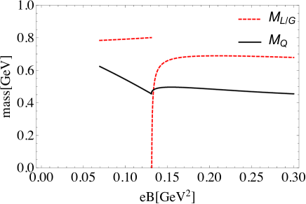
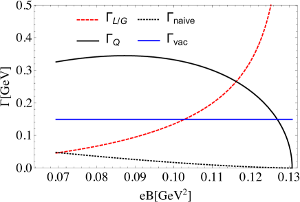
Figure 1: The magnetic-dependences of the rho masses (left panel) and widths (right panel) in the LLL approximation. In the right panel the naive expectation of the magnetic dependence on the decay width following from Eq.(I.2) has also been displayed together with the vacuum-width value estimated from Eq.(I.1).

We first discuss the magnetic dependences of the decay widths of for $\rho^{(L/G)}$ and $\rho^{(Q)}$. As clearly seen in the right panel of Fig. 1, the magnetic dependence of the rho meson decay rate is more complicated than that expected from the naive observation (Eq.(I.2)): as the $eB$ scale gets larger than the lowest $eB\simeq 0.07\,{\rm GeV}^{2}$, both the $\rho^{(L/G)}$ and $\rho^{(Q)}$ widths start to increase. As to the $\rho^{(Q)}$ width, it reaches a peak at around $eB\simeq 0.09\,{\rm GeV}^{2}$ to go down after that, while the $\rho^{(L/G)}$ width develops the size monotonically. At the critical magnetic scale $eB_{c}=(m_{\rho}^{2}-4m_{\pi}^{2})/4\simeq 0.13\,{\rm GeV}^{2}$, the difference in magnetic dependences drastically gets prominent: the $\rho^{(L/G)}$ width diverges at the critical point, while the $\rho^{(Q)}$ width goes to zero. These tendencies can be understood from Eq.(LABEL:effmass): the decay width to the LLL pion, $\Gamma_{L/G}(\pi^{+}_{(l=0)}\pi^{-}_{(l=0)})$, develops like

$$\Gamma_{L/G}(\pi^{+}_{(l=0)}\pi^{-}_{(l=0)})\sim\frac{(eB)^{2}}{\sqrt{m_{\rho}^{2}-4(m_{\pi}^{2}+eB)}}\,,$$ (IV.26)

which diverges at the critical point $eB_{c}$, while the $\Gamma_{Q}(\pi^{+}_{(l=0)}\pi^{-}_{(l=0)})$ scales like

$$\Gamma_{Q}(\pi^{+}_{(l=0)}\pi^{-}_{(l=0)})\sim(eB)\sqrt{m_{\rho}^{2}-4(m_{\pi}^{2}+eB)}\,,$$ (IV.27)

which has the peak (at around $eB\simeq 0.09\,{\rm GeV}^{2}$). This discrepant tendency would actually imply the difference in the polarization (spin) sensitivity related to the Landau-level number conservation, as will be discussed later.

As to the magnetic dependence of the $\rho^{(L/G)}$ and $\rho^{(Q)}$ masses, actually, it looks somewhat complicated compared to the widths as depicted in the left panel of Fig. 1: below the critical magnetic scale $eB_{c}\simeq 0.13\,{\rm GeV}^{2}$, $M_{L/G}$ gets larger, while $M_{Q}$ becomes smaller as the $eB$ increases from the lowest value $\simeq 0.07\,{\rm GeV}^{2}$. This is thought to happen due to the net contributions coming from the complicated functional forms at around the lowest magnetic scale (see Eq.(LABEL:effmass). At the critical point $eB_{c}$, the discrepancy in magnetic dependences for $M_{L/G}$ and $M_{Q}$ drastically gets large: the $M_{L/G}$ becomes non-analytic at the critical point, while the $M_{Q}$ still looks continuous. The discontinuity for $M_{L/G}$ is actually related to the ill behavior for the $\rho_{L/G}$ decay width at the critical point (see Eq.(IV.23) and the right panel of Fig. 1). Above the critical magnetic scale $eB_{c}\simeq 0.07\,{\rm GeV}^{2}$, the effect of the magnetic-dimensional reduction looks fairly mild for both $M_{L/G}$ and $M_{Q}$. (Actually, this tendency will be altered when one could ideally increase the magnetic field up to the scale above the upper limit $eB\sim 1\,{\rm GeV}^{2}$ in Eq.(IV.24): looking at Eq.(LABEL:effmass) one can easily see that the asymptotic behaviors of $M_{L/G}$ and $M_{Q}$, in the strong magnetic field limit, go like $M_{L/G}^{2}\sim-eB$ and $M_{Q}^{2}\sim+eB$.)

V Discussion

In the previous section we have numerically evaluated the magnetic-dependences of the rho mass and decay width, which are classified with respect to the rho-meson polarization structures including the effect of the magnetic-dimensional reduction. In this section, we shall discuss possible interpretations for our findings from several views of the field theoretical ground.

V.1 Moving onto the rest-frame representation

We have so far analyzed the rho meson masses and decay rates by decomposing the polarization states defined in an active frame where the rho mesons are energetically moving in the three-space dimension (see Eq.(III.16)). Instead, we shall here choose a rest frame, in which the rho meson has zero three-space momentum ($\vec{p}=\vec{0}$), to rephrase the results in the previous section, in terms of spin associated with the magnetic-direction, $s_{z}$. This would help us make comparison with other works based on the $s_{z}$-spin component.

To this end, we use the following polarization vectors irreducibly decomposed with respect to the $s_{z}$:

$$\epsilon_{1}^{\mu} = \frac{1}{\sqrt{2}}(0,1,i,0)\;\;\;\;\;\;(s_{z}=1,\;\;\;{\rm for}\;\rho^{0})\,,$$

$$\epsilon_{2}^{\mu} = \frac{1}{\sqrt{2}}(0,1,-i,0)\;\;\;(s_{z}=-1,\;\;\;{\rm for}\;\rho^{0})\,,$$

$$b^{\mu} = (0,0,0,1)\;\;\;\;\;\;\;\;\;\;\;(s_{z}=0,\;\;\;{\rm for}\;\rho^{0})\,,$$

$$u^{\mu} = (1,0,0,0)\,.$$ (V.28)

The inversed-propagator of the rho meson is then decomposed into the form:

$$D^{-1}_{\mu\nu}(p^{t},\vec{0}) = m_{\rho}^{2}g_{\mu\nu}-(p^{t})^{2}g_{\mu\nu}+\left(p^{t}\right)^{2}u_{\mu}u_{\nu}+\Pi_{||}^{S}(p^{t},\vec{0})(u^{\mu}u^{\nu}-b^{\mu}b^{\nu})$$ (V.29)

$$-\Pi_{||}^{T}(p^{t},\vec{0})p_{t}^{2}b_{\mu}b_{\nu}-\Pi_{\perp}^{S}(p^{t},\vec{0})(\epsilon^{*}_{1\mu}\epsilon_{1\nu}+\epsilon^{*}_{\mu 2}\epsilon_{2\nu})\,.$$

The corresponding $\rho^{0}$ meson propagator can be expressed by using the polarization vectors in Eq.(V.28) to be

$$D_{\mu\nu}=D^{(s_{z}=+1)}\epsilon^{*\mu}_{1}\epsilon^{\nu}_{1}+D^{(s_{z}=-1)}\epsilon^{*\mu}_{2}\epsilon^{\nu}_{2}+D^{(s_{z}=0)}b_{\mu}b_{\nu}+D^{(u)}u_{\mu}u_{\nu}\,.$$ (V.30)

Consequently, $D^{(s_{z}=+1)},D^{(s_{z}=-1)},D^{(s_{z}=0)}$ and $D^{(u)}$ are obtained as the functions of $\Pi$s as

$$D^{(s_{z}=+1)} = \frac{i}{m_{\rho}^{2}-p^{2}_{t}+\Pi_{\perp}^{S}(p^{t},\vec{0})}\,,$$

$$D^{(s_{z}=-1)} = \frac{i}{m_{\rho}^{2}-p^{2}_{t}+\Pi_{\perp}^{S}(p^{t},\vec{0})}\,,$$

$$D^{(s_{z}=0)} = \frac{i}{m_{\rho}^{2}-p^{2}_{t}+\Pi_{||}^{S}(p^{t},\vec{0})+\Pi_{||}^{T}(p^{t},\vec{0})p_{t}^{2}}\,,$$

$$D^{(u)} = \frac{i}{m_{\rho}^{2}+\Pi_{||}^{S}(p^{t},\vec{0})}\,.$$ (V.31)

It is obvious from Eqs.(III.17) and (V.31) that the masses and widths for the physical spin-1 modes $(D^{(s_{z}=\pm 1,0)})$ are respectively identical to those for the physical-active polarization modes ($D^{L,G,Q}$), namely,

$$M_{L/G}=M_{(s_{z}=\pm 1)}\,,\qquad M_{Q}=M_{(s_{z}=0)}\,,$$

$$\Gamma(\rho^{(L/G)}\to\pi^{+}_{(l=0)}\pi^{-}_{(l=0)})=\Gamma(\rho^{(s_{z}=\pm 1)}\to\pi^{+}_{(l=0)}\pi^{-}_{(l=0)})\,,$$

$$\Gamma(\rho^{(Q)}\to\pi^{+}_{(l=0)}\pi^{-}_{(l=0)})=\Gamma(\rho^{(s_{z}=0)}\to\pi^{+}_{(l=0)}\pi^{-}_{(l=0)})\,.$$ (V.32)

Thus, the results on the $\rho^{(L/G)}$ and $\rho^{(Q)}$ obtained in the previous section can be reinterpreted as those for the $\rho^{(s_{z}=\pm 1)}$ and $\rho^{(s_{z}=0)}$, respectively.

V.2 Polarization (spin)-dependence sensitive to Landau-level number-conservation?

In the previous section, Sec. IV, we observed somewhat ill behaviors for the $\rho^{(L/G)}$ meson (i.e. $\rho^{(s_{z}=\pm 1)}$): the discontinuity for the mass and the divergence for the widths at the critical magnetic scale $eB_{c}\simeq 0.13\,{\rm GeV}^{2}$ (see Fig. 1). As to this result, here we shall address a possible interpretation in relation to the Landau-level number-conservation.

First of all, once encountering such an ill tendency, one might simply think that the wavefunction-renormalization factor ($Z^{(L/G)}$) should diverge at the point (see the width formula in Eq.(III.21)). In the present situation, however, it is not the case: we have explicitly checked that the $Z^{(L/G)}$ keeps finite values even at the critical magnetic scale. Therefore, the ill behavior seems to have nothing to do with the wavefunction-renormalization factor.

Now we would suspect that the issue could be related to the conservation of the Landau-level number: actually, if going beyond the LLL approximation in evaluating the pion-loop integral, one could find that terms involving pions carrying different Landau levels are present in the $(L/G)$-polarization ($s_{z}=\pm 1$) state of the rho meson. Note from Eq.(III.16) that only the $L/G$ polarization mode carries the spatial-momentum perpendicular ($\perp$) to the magnetic field, which contaminates the Landau-level number conservation when couples to pions via the $\rho-\pi-\pi$ vertex like $\rho_{\perp}\pi^{+}_{(l_{1})}\partial_{\perp}\pi^{-}_{(l_{2})}$, resulting in the Landau-level number violation. Thus, the ill behavior about the $\rho^{(L/G)}$ (or $\rho^{(s_{z}=\pm 1)}$) may be understood by the disastrous breaking of the Landau-level number, which originates from the naive LLL truncation, hence the result on this polarization mode may be unreliable at this moment.

The well-defined magnetic-dependence of the $\rho^{(L/G)}$ would be obtained when one fully sums up the infinite tower of the Landau levels.

In contrast, the polarization mode of the $\rho^{(Q)}$ (or $\rho^{(s_{z}=0)}$), which accompanies only the momentum parallel to the magnetic field (see Eq.(III.16)), is harmless against the Landau-level number conservation because there does not exist a coupling form like $\rho_{||}\pi^{+}_{(l_{1})}\partial_{\perp}\pi^{-}_{(l_{2})}$ breaking the Landau-level number when couples to pions. Thus, to this polarization mode, the LLL truncation is safely doable, hence we might have arrived at the well-defined magnetic-dependences as seen from Fig. 1.

Consequently, the result on the lifetime, the inverse of $\Gamma(\rho^{(Q)}(\rho^{(s_{z}=0)})\to\pi^{+}_{(l=0)}\pi^{-}_{(l=0)})$ in Fig. 1 and Eq.(IV.23), is manifestly physical: recall the constrained region of the magnetic scale in Eq.(IV.25) up to the critical scale ($eB_{c}\simeq 0.13\,{\rm GeV}^{2}$), $0.07\lesssim eB\lesssim 0.13\,{\rm GeV}^{2}$, which only allows the decay channel to the LLL-charged pion pair, namely,

$$\Gamma(\rho^{(Q)}(\rho^{(s_{z}=0)})\to\pi^{+}_{(l=0)}\pi^{-}_{(l=0)})=\Gamma(\rho^{(Q)}(\rho^{(s_{z}=0)})\to\pi^{+}\pi^{-})\,,$$ (V.33)

where $\pi^{\pm}$ include the full Landau-level tower. This clearly suggests a new “fate” of the rho meson in the magnetic field, which would be more complicated than the naive expectation followed from Eq.(I.2), as displayed in the right panel of Fig. 1.

Unlike the case of the lifetime, the mass of the $\rho^{(Q)}$ ($\rho^{(s_{z}=0)}$) might get significant contributions from the higher Landau-levels even in the present restricted magnetic domain, $0.07\lesssim eB\lesssim 0.13\,{\rm GeV}^{2}$. One could compare the present result on the $\rho^{(s_{z}=0)}$ mass with other works in Refs. Luschevskaya:2012xd ; Andreichikov:2013zba ; Luschevskaya:2014lga ; Liu:2014uwa ; Luschevskaya:2015bea ; Andreichikov:2016ayj . To make a conclusive answer to the validity of the LLL approximation for the mass estimation, one would need more rigorous argument including higher Landau levels.

The full computations regarding the $\rho^{(L/G)}$ mode including the infinite tower of the Landau levels would be also of importance, to be pursued in the future work.

VI Summary

In summary, we have attempted to access the naive expectation on the lifetime of the neutral rho meson in the magnetic field (Eq.(I.2)), by explicitly computing the charged pion loop correction to the neutral rho meson propagator based on a chiral effective model. To see the significance of the magnetic-dimensional reduction-effect, we simply took the LLL approximation. We found that the magnetic field significantly separates the rho-meson polarization states in a nontrivial way, compared to the vacuum case, which is due to the magnetic-dimensional reduction (Eqs.(III.16) and (III.17)). According to the intrinsic polarization decomposition, the neutral rho mass and width are split as well, so the magnetic-dependences show up with respect to the polarization (spin) modes, labeled by $L/G$ and $Q$, or $s_{z}=\pm 1,0$ for the physical modes. Then we numerically evaluated the magnetic-dependences of the masses and the widths respectively for the polarization (spin) modes. Of particular interest is that as the magnetic field increases, the rho width for the spin $s_{z}=0$ starts to develop, reach a peak, to be vanishing at the critical magnetic field to which the folklore refers (Fig. 1). This result is exact at the LLL approximation (Eq.(V.33)), and would suggest that the life of the neutral rho meson in the magnetic field may be more complicated than the naive expectation.

A possible correlation between the spin-dependent magnetic scaling, the Landau-level number-conversation and the validity of the LLL approximation was also discussed.

Note added: After completion of the present manuscript, we noticed a paper (arXiv:1610.07887), in which a similar computation on the charged pion loop contribution to the neutral rho meson decay width has been made. In that paper, the spin-dependent decomposition due to the magnetic-dimensional reduction has not clearly been addressed, though, some portion of what we found in the present paper might be overlapped with theirs.

Appendix A The Feynman parameter integrals

In this Appendix we present the Feynman parameter integrals relevant to the evaluation of the charged pion loop diagram in Sec. III.

$$\int_{0}^{1}dx\ln\frac{\Lambda^{2}}{\Delta}=\begin{cases}\ln\Lambda^{2}+2-\ln\left(m^{2}_{\pi}+eB\right)-\frac{2}{\sqrt{p^{2}_{||}}}\sqrt{4(m^{2}_{\pi}+eB)-p^{2}_{||}}\arctan\sqrt{\frac{p^{2}_{||}}{4m^{2}_{\pi}+eB-p^{2}_{||}}}\\ \,\,\,\,\,\,\,\,\,\,\,\,\,\,\,\,\,\,\,\,\,\,\,\,\,\,\,\,\,\,\,\,\,\,\,\,\,\,\,\,\,\,\,\,\,\,\,\,\,\,\,\,\,\,\,\,\,\,\,\,\,\,\,\,\,\,\,\,\,\,\,\,\,\,\,\,\,\,\,\,\,\,\,\,\,\,\,\,\,\,\,\,\,\,\,\,\,\,\,\,\,\,\,\,\,\,\,\,\,\,\,\,\,\,\,\,\,\,\,\,\,\,\,\,\,\,\,\,\,\,\,\,\,\,\,\left({\rm for}\,\,\,p_{||}^{2}<4(m_{\pi}^{2}+eB)\right)\\ \\ \ln\Lambda^{2}+2-\ln\left(m^{2}_{\pi}+eB\right)-\frac{2}{\sqrt{p^{2}_{||}}}\sqrt{p^{2}_{||}-4(m^{2}_{\pi}+eB)}\Biggl{[}\ln\frac{\sqrt{p^{2}_{||}-4(m^{2}_{\pi}+eB)}+\sqrt{p^{2}_{||}}}{2\sqrt{m_{\pi}^{2}+eB}}-i\pi\Biggl{]}\\ \,\,\,\,\,\,\,\,\,\,\,\,\,\,\,\,\,\,\,\,\,\,\,\,\,\,\,\,\,\,\,\,\,\,\,\,\,\,\,\,\,\,\,\,\,\,\,\,\,\,\,\,\,\,\,\,\,\,\,\,\,\,\,\,\,\,\,\,\,\,\,\,\,\,\,\,\,\,\,\,\,\,\,\,\,\,\,\,\,\,\,\,\,\,\,\,\,\,\,\,\,\,\,\,\,\,\,\,\,\,\,\,\,\,\,\,\,\,\,\,\,\,\,\,\,\,\,\,\,\,\,\,\,\,\,\left({\rm for}\,\,\,4(m_{\pi}^{2}+eB)<p^{2}_{||}\right)\,,\end{cases}$$

$$\int_{0}^{1}dx\frac{1}{\Delta}=\begin{cases}\frac{4}{\sqrt{p^{2}_{||}}\sqrt{4(m^{2}_{\pi}+eB)-p^{2}_{||}}}\arctan\left(\frac{p^{2}_{||}}{\sqrt{p^{2}_{||}}\sqrt{4(m^{2}_{\pi}+eB)-p^{2}_{||}}}\right)\,\,\,\,\,\,\,\,\,\,\,\,\,\,\,\left({\rm for}\,\,\,p_{||}^{2}<4(m_{\pi}^{2}+eB)\right)\\ \\ \frac{1}{\sqrt{p^{2}_{||}}\sqrt{p^{2}_{||}-4(m_{\pi}^{2}+eB)}}\Biggl{[}-4\ln\frac{\sqrt{p^{2}_{||}-4(m_{\pi}^{2}+eB)}+\sqrt{p^{2}_{||}}}{2\sqrt{m_{\pi}^{2}+eB}}+2i\pi\Biggl{]}\,\,\,\,\,\,\,\,\,\,\,\,\,\,\,\left({\rm for}\,\,\,4(m_{\pi}^{2}+eB)<p_{||}^{2}\right)\,,\end{cases}$$ (A.35)

where $\Delta=x(x-1)p_{||}^{2}+m_{\pi}^{2}+eB$.

References

• (1) D. E. Kharzeev, L. D. McLerran and H. J. Warringa, Nucl. Phys. A 803, 227 (2008) doi:10.1016/j.nuclphysa.2008.02.298 [arXiv:0711.0950 [hep-ph]].
• (2) V. Skokov, A. Y. Illarionov and V. Toneev, Int. J. Mod. Phys. A 24, 5925 (2009) doi:10.1142/S0217751X09047570 [arXiv:0907.1396 [nucl-th]].
• (3) A. K. Harding and D. Lai, Rept. Prog. Phys.  69, 2631 (2006) doi:10.1088/0034-4885/69/9/R03 [astro-ph/0606674].
• (4) J. M. Lattimer and M. Prakash, Phys. Rept.  442, 109 (2007) doi:10.1016/j.physrep.2007.02.003 [astro-ph/0612440].
• (5) A. Y. Potekhin, Phys. Usp.  53, 1235 (2010) [Usp. Fiz. Nauk 180, 1279 (2010)] doi:10.3367/UFNe.0180.201012c.1279 [arXiv:1102.5735 [astro-ph.SR]].
• (6) D. Lai, Space Sci. Rev.  191, no. 1-4, 13 (2015) doi:10.1007/s11214-015-0137-z [arXiv:1411.7995 [astro-ph.HE]].
• (7) J. S. Schwinger, Phys. Rev.  82, 664 (1951). doi:10.1103/PhysRev.82.664.
• (8) A. Ayala, A. Sanchez, G. Piccinelli and S. Sahu, Phys. Rev. D 71, 023004 (2005) doi:10.1103/PhysRevD.71.023004 [hep-ph/0412135].
• (9) V. I. Ritus, Annals Phys.  69, 555 (1972). doi:10.1016/0003-4916(72)90191-1.
• (10) A. E. Shabad, Annals Phys.  90, 166 (1975). doi:10.1016/0003-4916(75)90144-X.
• (11) K. Hattori and K. Itakura, Annals Phys.  330, 23 (2013) doi:10.1016/j.aop.2012.11.010 [arXiv:1209.2663 [hep-ph]].
• (12) K. A. Olive et al. [Particle Data Group Collaboration], Chin. Phys. C 38, 090001 (2014). doi:10.1088/1674-1137/38/9/090001.
• (13) E. V. Luschevskaya and O. V. Larina, Nucl. Phys. B 884, 1 (2014) doi:10.1016/j.nuclphysb.2014.04.003 [arXiv:1203.5699 [hep-lat]].
• (14) M. A. Andreichikov, B. O. Kerbikov, V. D. Orlovsky and Y. A. Simonov, Phys. Rev. D 87, no. 9, 094029 (2013) doi:10.1103/PhysRevD.87.094029 [arXiv:1304.2533 [hep-ph]].
• (15) E. V. Luschevskaya, O. E. Solovjeva, O. A. Kochetkov and O. V. Teryaev, Nucl. Phys. B 898, 627 (2015) doi:10.1016/j.nuclphysb.2015.07.023 [arXiv:1411.4284 [hep-lat]].
• (16) H. Liu, L. Yu and M. Huang, Phys. Rev. D 91, no. 1, 014017 (2015) doi:10.1103/PhysRevD.91.014017 [arXiv:1408.1318 [hep-ph]].
• (17) E. V. Luschevskaya, O. A. Kochetkov, O. V. Teryaev and O. E. Solovjeva, JETP Lett.  101, no. 10, 674 (2015). doi:10.1134/S0021364015100094.
• (18) M. A. Andreichikov, B. O. Kerbikov, E. V. Luschevskaya, Y. A. Simonov and O. E. Solovjeva, arXiv:1610.06887 [hep-ph].