Vortex-antivortex proliferation from an obstacle in thin film ferromagnets

Abstract

Magnetization dynamics in thin film ferromagnets can be studied using a dispersive hydrodynamic formulation. The equations describing the magnetodynamics map to a compressible fluid with broken Galilean invariance parametrized by the longitudinal spin density and a magnetic analog of the fluid velocity that define spin-density waves. A direct consequence of these equations is the determination of a magnetic Mach number. Micromagnetic simulations reveal nucleation of nonlinear structures from an impenetrable object realized by an applied magnetic field spot or a defect. In this work, micromagnetic simulations demonstrate vortex-antivortex pair nucleation from an obstacle. Their interaction establishes either ordered or irregular vortex-antivortex complexes. Furthermore, when the magnetic Mach number exceeds unity (supersonic flow), a Mach cone and periodic wavefronts are observed, which can be well-described by solutions of the steady, linearized equations. These results are reminiscent of theoretical and experimental observations in Bose-Einstein condensates, and further supports the analogy between the magnetodynamics of a thin film ferromagnet and compressible fluids. The nucleation of nonlinear structures and vortex-antivortex complexes using this approach enables the study of their interactions and effects on the stability of spin-density waves.

I Introduction

Magnetization dynamics in thin film ferromagnets provide an exciting platform to study nonlinear wave phenomena. This is possible due to the exchange interaction that confers ferromagnetic order and wave dispersion, nonlinear effects such as anisotropy, and diverse mechanisms available to excite magnetization dynamics Stör and Siegmann (2006). In fact, coherent nonlinear magnetization structures were observed many decades ago, such as domain walls and vortices Hubert and Schäfer (2009). More recently, envelope solitons Tong et al. (2010); Wang et al. (2014), dissipative droplets Hoefer, Silva, and Keller (2010); Mohseni et al. (2013); Iacocca et al. (2014); Macià, Backes, and Kent (2014); Chung et al. (2016), and skyrmions Romming et al. (2013); Sampaio et al. (2013); Zhou et al. (2015); Jiang et al. (2015) have also been observed in these materials. Another class of nonlinear structure in thin film ferromagnets is a spatially periodic, superfluid-like texture or soliton lattice König, Bønsager, and MacDonald (2001); Sonin (2010); Takei and Tserkovnyak (2014); Chen et al. (2014); Iacocca, Silva, and Hoefer (2017) that is able to carry spin currents due to its nontrivial topology, opening new pathways to nonlinear phenomena and potential applications.

Recently, superfluid-like magnetic states have been interpreted in the context of hydrodynamics Halperin and Hohenberg (1969); Iacocca, Silva, and Hoefer (2017). It was shown that the Landau-Lifshitz (LL) equation describing magnetodynamics can be exactly cast as dispersive hydrodynamic equations, reminiscent of those describing Bose-Einstein condensates (BECs) Pethick and Smith (2002) and other superfluid-like media El and Hoefer (2016). An additional, direct, exact connection between polarization waves in two-component BECs Stamper-Kurn and Ueda (2013) and magnetization dynamics has recently been identified Qu, Pitaevskii, and Stringari (2016); Congy, Kamchatnov, and Pavloff (2016). From the magnetic dispersive hydrodynamic formulation, it is possible to characterize superfluid-like states as dynamic, uniform hydrodynamic states (UHSs) or static, spin-density waves (SDWs) parametrized by a longitudinal spin density $n$ and fluid velocity $\mathbf{u}$ proportional to the spatial gradient of the magnetization’s in-plane phase. By defining the magnetic analog of the Mach number from classical gas dynamics, $\mathrm{M}$, subsonic and supersonic flow conditions can be identified. Interestingly, this magnetic fluid representation, due to ferromagnetic exchange coupling, generally exhibits broken Galilean invariance at the level of (linear) spin wave excitations Iacocca, Silva, and Hoefer (2017). Consequently, the physics are reference-frame-dependent. This is in stark contrast to the velocity-dependent dynamics of localized, topological textures that result from their inherent nonlinearity Yamada et al. (2007); Beach, Tsoi, and Erskine (2008).

Intriguing dynamics result from the interaction between a superfluid-like state and a finite-sized obstacle. Micromagnetic simulations Iacocca, Silva, and Hoefer (2017) demonstrated that, in general, SDWs ($\mathbf{u}\neq 0$) at subsonic conditions, $\mathrm{M}<1$, flow in a stable, laminar fashion around a point defect whereas a Mach cone, wavefronts, and irregular vortex-antivortex (V-AV) pair nucleation takes place at supersonic conditions, $\mathrm{M}>1$. In the different regime of thick, homogeneous ferromagnets ($\mathbf{u}=0$), “spin-Cerenkov” radiation was observed in the moving reference frame Yan et al. (2013). In classical fluids, similar coherent structures can be nucleated from an obstacle. The conditions defining the onset of specific features usually depend on the flow velocity or, equivalently, the Mach number. At subsonic conditions, obstacles can nucleate vortices resulting from an unsteady wake Williamson (1996); Leweke, Le Dizès, and Williamson (2016). A common example is the von Kármán vortex street, characterized by a train of vortices of alternating circulation. This has been thoroughly studied as a function of the Reynolds number for viscous, incompressible fluids Williamson (1996). At supersonic conditions for a compressible gas, a Mach cone can be generated as typified by a jet breaking the speed of sound.

In contrast, superfluids such as BECs exhibit important differences. Firstly, vortices are quantized due to irrotational flow and secondly, BECs are compressible and inviscid. Therefore, a Reynolds number is not defined in the sense of classical fluids. However, it has been suggested that an alternative superfluid Reynolds number can be defined from the onset of quantum vortex shedding Reeves et al. (2015). In fact, V-AV pair dynamics can occur in superfluids as their numerical nucleation Frisch, Pomeau, and Rica (1992) and instability Nore, Brachet, and Fauve (1993) were demonstrated at subsonic conditions. Numerical studies also identified the existence of a von Kármán like vortex street Sasaki, Suzuki, and Saito (2010), which has been recently demonstrated experimentally Kwon et al. (2016). At supersonic conditions, Mach cones have been observed, both theoretically and experimentally, accompanied by wave radiation or wavefronts ahead of the obstacle Carusotto et al. (2006); Gladush et al. (2007) and, at large $\mathrm{M}$, steady, oblique dark solitons can be generated inside the Mach cone El, Gammal, and Kamchatnov (2006).

The similarity between the equations describing BECs and thin film ferromagnetic magnetodynamics suggests that the latter may support the many structures mentioned above, with the possibility of new phenomena due to a ferromagnet’s more complex geometry. The stability of SDWs in a finite, thin film ferromagnet may be impacted by V-AV nucleation. It is known that V-AV pairs in magnets can excite spin waves by diverse annihilation processes Hertel and Schneider (2006), e.g., V-AV interaction with other V-AVs, with defects, or with physical boundaries. To explore the existence, dynamics, and stability of nonlinear structures in thin film ferromagnets, we study analytically and numerically the interaction between a SDW and an impenetrable, finite-sized obstacle or defect.

In this paper, we show that in the static, laboratory reference frame, trains of V-AV pairs nucleated by a sufficiently large obstacle exhibit stable, linear motion at subsonic conditions whereas irregular V-AV dynamics are observed at supersonic conditions. This is due to the V-AV translation imposed by the underlying fluid velocity and the interactions between vortices, leading to translational instabilities or even V-V and AV-AV rotation. In the moving reference frame with zero fluid velocity, V-AV pairs generally annihilate, leading to irregular dynamics. However, at supersonic conditions, V-AV pairs exhibit structure by describing an oblique path inside the Mach cone. Wavefronts are observed to nucleate ahead of the obstacle in both reference frames at supersonic conditions. For thin film ferromagnets with finite extent, the observed nonlinear structures are transient as the system relaxes to an energy minimum. These results are not only relevant for the stability of a SDW but they also represent a cornerstone to study V-AV complexes and their interaction with other nonlinear structures. More generally, our work provides an avenue to study the proliferation of topological textures in magnetism. For example, recent numerical results have demonstrated the generation of skyrmions by spin-transfer torque from anisotropic obstacles Everschor-Sitte et al. (2016), similar to the linear V-AV vortex motion we show below.

The paper is organized as follows. Section II summarizes the hydrodynamic formulation of the Landau-Lifshitz equation. The magnetic dispersive hydrodynamic equations obtained in section II are compared to the equations describing the mean field dynamics of BECs and two-component BECs in section III. In section IV, we use a linearized analysis to predict some properties of the patterns supported by the dispersive hydrodynamic flow past an obstacle. We also use analogies to classical fluids and superfluids to identify common flow patterns. Section V describes the results obtained from micromagnetic simulations. Finally, we provide our concluding remarks in section VI.

II Dispersive hydrodynamic formulation

Following the formulation outlined in Ref. Iacocca, Silva, and Hoefer, 2017, the magnetization dynamics of a thin film ferromagnet with planar anisotropy can be conveniently described by the nondimensionalized LL equation

$$\frac{\partial\mathbf{m}}{\partial t}=-\mathbf{m}\times\mathbf{h}_{\mathrm{eff}}-\alpha\mathbf{m}\times\mathbf{m}\times\mathbf{h}_{\mathrm{eff}},$$ (1)

with an effective field given by

$$\mathbf{h}_{\mathrm{eff}}=\Delta\mathbf{m}-m_{z}\hat{\mathbf{z}}+h_{0}\hat{\mathbf{z}},$$ (2)

including, respectively, the ferromagnetic exchange field, a local (zero-thickness limit) dipolar field, and a perpendicular external field. The dispersive hydrodynamic equations are obtained by inserting the transformation to Hamiltonian variables Papanicolaou and Tomaras (1991)

$$n=m_{z},\quad\mathbf{u}=-\nabla\Phi=-\nabla\left[\arctan{\left(m_{y}/m_{x}\right)}\right],$$ (3)

into Eq. (1), where $|n|\leq 1$ is the longitudinal spin density ($|n|=1$ corresponds to the vacuum state) and $\mathbf{u}$ is the curl-free (irrotational) fluid velocity. First, we exactly solve for $\partial\Phi/\partial t$ and obtain

$$\frac{\partial\Phi}{\partial t} = -(1-|\mathbf{u}|^{2})n+\frac{\Delta n}{1-n^{2}}+\frac{n|\nabla n|^{2}}{(1-n^{2})^{2}}$$ (4)

$$+h_{0}-\frac{\alpha}{1-n^{2}}\nabla\cdot[(1-n^{2})\mathbf{u}].$$

The gradient of Eq. (4) and the equation for $n$ are

$$\frac{\partial n}{\partial t} = \nabla\cdot\left[(1-n^{2})\mathbf{u}\right]+\alpha(1-n^{2})\frac{\partial\Phi}{\partial t},$$ (5a)

$$\frac{\partial\mathbf{u}}{\partial t} = \nabla\left[(1-|\mathbf{u}|^{2})n\right]-\nabla\left[\frac{\Delta n}{1-n^{2}}+\frac{n|\nabla n|^{2}}{(1-n^{2})^{2}}\right]$$ (5b)

$$-\nabla h_{0}+\alpha\nabla\left[\frac{1}{1-n^{2}}\nabla\cdot\left[(1-n^{2})\mathbf{u}\right]\right].$$

These are an exact transformation of the LL equation, Eq. (1), and fully describe the magnetization dynamics.

The ground-state solutions of Eqs. (5a) and (5b) are static magnetization textures known as spin-density waves (SDWs), such that

$$\frac{\partial\Phi}{\partial t}=\Omega=-(1-\bar{u}^{2})\bar{n}+h_{0}=0$$ (6)

where the longitudinal spin density and fluid velocity, $(n,\mathbf{u})=(\bar{n},\bar{u}\hat{\mathbf{x}})$, are constant. This implies that the SDW can have a constant out-of-plane tilt and a periodic, in-plane spatial rotation of the azimuthal angle $\Phi$. For simplicity, we consider a non-negative fluid velocity along $\hat{\mathbf{x}}$, i.e., $\bar{u}>0$.

The static condition Eq. (6) at a finite field corresponds to the ground state SDW conditions imposed by magnetic damping. If by some means $\Omega\neq 0$ in Eq. (6), e.g., by an abrupt jump in the field $h_{0}$ to another value $h_{1}$, the associated dynamic solutions are considered UHSs Iacocca, Silva, and Hoefer (2017) that undergo a slow relaxation to a SDW. This relaxation process for $\bar{n}(t)$ maintains constant $\bar{u}$ and can be computed by assuming spatial uniformity in Eqs. (5a) resulting in the temporal differential equation for the longitudinal spin density

$$\frac{d\bar{n}}{dt}=-\alpha(1-\bar{u}^{2})(1-\bar{n}^{2})\left(\bar{n}-\frac{h_{1}}{1-\bar{u}^{2}}\right).$$ (7)

Upon integration, Eq. (7) yields the implicit relationship

$$\left[\frac{\left(\bar{n}-\frac{h_{1}}{1-\bar{u}^{2}}\right)^{2}}{1-\bar{n}^{2}}\right]^{1-\bar{u}^{2}}\left(\frac{1+\bar{n}}{1-\bar{n}}\right)^{h_{1}}=C\exp\left\{-2\alpha\left[(1-\bar{u}^{2})^{2}-h_{1}^{2}\right]t\right\},$$ (8)

for $\bar{n}(t)$, where the constant $C$ is determined from the initial density $\bar{n}_{0}=h_{0}/(1-\bar{u}^{2})$. This expression composes an exponential decay of the density to the static state $\bar{n}(t)\to\bar{n}_{1}=h_{1}/(1-\bar{u}^{2})$, $t\to\infty$ for any initial $\bar{u}$.

To study the dynamics originating from the interaction between a SDW and an obstacle, it is important to characterize small-amplitude perturbations of the SDW, described by the generalized spin wave dispersion relation

$$\omega_{\pm}=\left(2\bar{n}\mathbf{u}-\mathbf{V}\right)\cdot\mathbf{k}\pm|\mathbf{k}|\sqrt{(1-\bar{n}^{2})(1-\bar{u}^{2})+|\mathbf{k}|^{2}},$$ (9)

where $\mathbf{k}$ is the wave vector and $\mathbf{V}$ is the velocity of an external observer or Doppler shift. This generalized dispersion relation reduces to the typical Galilean invariant, exchange-mediated spin wave dispersion in the vacuum limit $|\bar{n}|\approx 1$. However, Galilean invariance is broken in general Iacocca, Silva, and Hoefer (2017), leading to reference-frame-dependent physics.

From Eq. (9), one can derive the generalized spin wave phase and group velocities, respectively, $v_{p}$ and $v_{g}$

$$\mathbf{v}_{p,\pm} = \frac{\omega_{\pm}}{|\mathbf{k}|}\hat{\mathbf{k}}$$

$$= \left[\left(2\bar{n}\mathbf{u}-\mathbf{V}\right)\cdot\hat{\mathbf{k}}\pm\sqrt{(1-\bar{n}^{2})(1-\bar{u}^{2})+|\mathbf{k}|^{2}}\right]\hat{\mathbf{k}},$$

$$\mathbf{v}_{g,\pm} = \nabla_{\mathbf{k}}\omega_{\pm}\hat{\mathbf{k}}$$

$$= \left[\left(2\bar{n}\mathbf{u}-\mathbf{V}\right)\cdot\hat{\mathbf{k}}\pm\frac{(1-\bar{n}^{2})(1-\bar{u}^{2})+2|\mathbf{k}|^{2}}{\sqrt{(1-\bar{u}^{2})(1-\bar{n}^{2})+|\mathbf{k}|^{2}}}\right]\hat{\mathbf{k}}.$$

The long-wavelength limit $|\mathbf{k}|\rightarrow 0$ leads to coincident phase and group velocities, $\mathbf{v}_{p}=\mathbf{v}_{g}$, corresponding to the magnetic sound speeds imposed by the SDW

$$s_{\pm}=2\bar{n}\bar{u}+\bar{V}\pm\sqrt{(1-\bar{n}^{2})(1-\bar{u}^{2})},$$ (11)

where we have assumed $\mathbf{V}=-\bar{V}\hat{\mathbf{x}}$ and $\hat{\mathbf{k}}=\hat{\mathbf{x}}$ for simplicity.

Subsonic (counter-propagating waves) and supersonic (co-propagating waves) flow conditions can be identified from Eq. (11). In particular, the transition between these regimes, the sonic curve, occurs when $s_{-}=0$ or $s_{+}=0$ in Eq. (11), resulting in

$$\bar{V}\left(\bar{V}+4\bar{n}\bar{u}\right)=\left(1-\bar{n}^{2}\right)-\left(1+3\bar{n}^{2}\right)\bar{u}^{2}.$$ (12)

Equation (12) represents the sonic surface for any $\bar{V}$, $\bar{u}$, and $|\bar{n}|<1$, projections of which are shown in Fig. 1. Relatively simple expressions for Eq. (12) are available when we restrict to $\bar{V}=0$ or $\bar{u}=0$ (thicker lines in Fig. 1). Thus, we define the Mach numbers in these cases

$$\mathrm{M}_{u}=|\bar{u}|\sqrt{\frac{1+3\bar{n}^{2}}{1-\bar{n}^{2}}},\quad\mathrm{M}_{V}=\frac{|\bar{V}|}{\sqrt{1-\bar{n}^{2}}},$$ (13)

respectively, so that $\mathrm{M}=1$ corresponds to Eq. (12).

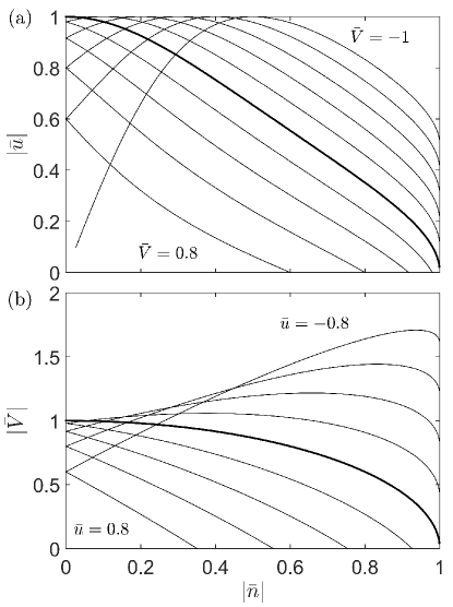
Figure 1: Sonic curves calculated from Eq. (12) by varying (a) $\bar{V}$ and (b) $\bar{u}$ in steps of $0.2$. The cases for (a) $\bar{V}=0$ and (b) $\bar{u}=0$ are emphasized by the thicker solid line, corresponding to Eq. (13).

III Bose-Einstein condensate limit of the dispersive hydrodynamic equations

The hydrodynamic equations governing the mean field dynamics of a BEC can be obtained as a limiting case of the magnetic, dispersive hydrodynamic equations, Eqs. (5a) and (5b). For this, one should consider the nearly perpendicular, small velocity, long-wavelength, and low-frequency expansion

$$n = 1-\epsilon\rho,\quad\mathbf{u}=\left(\frac{1}{2}\epsilon\right)^{1/2}\mathbf{v},$$

$$\tilde{\mathbf{x}} = \left(\frac{1}{2}\epsilon\right)^{1/2}\mathbf{x},\quad\tilde{t}=\epsilon t,\quad U=\epsilon h_{0},$$ (14)

where $0<\epsilon\ll 1$ measures the magnetization deviation from the perpendicular, vacuum state. Inserting this expansion into Eqs. (5a) and (5b) while keeping only the leading order terms and setting $\alpha=0$ results in

$$\frac{\partial\rho}{\partial\tilde{t}} + \tilde{\nabla}\cdot(\rho\mathbf{v})=0,$$ (15a)

$$\frac{\partial\mathbf{v}}{\partial\tilde{t}} + (\mathbf{v}\cdot\tilde{\nabla})\mathbf{v}+\tilde{\nabla}\rho=\frac{1}{4}\tilde{\nabla}\left[\frac{\tilde{\Delta}\rho}{\rho}-\frac{|\tilde{\nabla}\rho|^{2}}{2\rho^{2}}\right]-\tilde{\nabla}U,$$ (15b)

a non-dimensional form of the conservative, hydrodynamic equations of a repulsive BEC with trapping potential $U(\tilde{\mathbf{x}})$ (see, e.g., Ref. Pethick and Smith, 2002). From this analogy it follows that the “healing length” defined in BEC as the transition distance between two states with dissimilar density is simply given by the spatial scaling in ferromagnetic materials, i.e., the exchange length in the case of planar ferromagnets Iacocca, Silva, and Hoefer (2017).

BECs can lose superfluidity when its interaction with an obstacle results in the generation of small-amplitude waves Pethick and Smith (2002). This can be described in terms of the Landau criterion for superfluidity, which invokes Galilean invariance to find the conditions where spontaneous wave generation is energetically unfavorable. For a BEC described by Eq. (15), the Landau criterion is $|\mathbf{v}|<s$ where $s=\sqrt{\rho}$ is the BEC long wave speed of sound.

For BECs, the Landau criterion and the Mach number are closely related. Both describe the conditions for subsonic to supersonic flow transitions. The Mach number for BECs is Pethick and Smith (2002)

$$\mathrm{M}_{\mathrm{BEC}}=\frac{|\mathbf{v}|}{\sqrt{\rho}}.$$ (16)

The sonic curve, ${\mathrm{M}_{\mathrm{BEC}}=1}$, is the critical transition from subsonic to supersonic conditions and represents the breakdown of superfluidity, i.e., spontaneous wave generation is energetically favorable. It can be verified that the magnetic Mach numbers, Eq. (13), reduce to Eq. 16 for small deviation from vacuum, by use of the transformation (III). Since the standard derivation of the Landau criterion utilizes Galilean invariance, it can only be applied to exchange-mediated, Galilean invariant spin waves in a perpendicularly magnetized thin film ferromagnet. Away from this regime, SDWs break Galilean invariance Iacocca, Silva, and Hoefer (2017). The more general identification of the subsonic to supersonic transition as the breakdown of superfluidity, Eq. (13), is the appropriate one for SDWs because the generalized spin wave dispersion (9) exhibits non-zero curvature for positive wavenumbers.

It is important to stress that Eqs. (15) are conservative, so that the connection between BECs and exchange-mediated spin waves is valid insofar as magnetic damping is neglected. However, because damping is typically weak $0<\alpha\ll 1$, we can invoke conservative arguments to describe the dynamics and nucleated structures over sufficiently short timescales (proportional to $\alpha^{-1}$) when a finite-sized obstacle is introduced.

A more general analog to the magnetic, dispersive hydrodynamic equations, Eqs. (5a) and (5b), can be found in two-component Bose-Einstein condensates, a class of spinor Bose gases Stamper-Kurn and Ueda (2013) that possess magnetic properties. In particular, Congy et al. Congy, Kamchatnov, and Pavloff (2016) found that the polarization waves in a one-dimensional, two-component BEC can be described by approximate dispersive hydrodynamic equations coinciding exactly with the one-dimensional projection of Eqs. (5a) and (5b) when $\alpha=0$. This suggests that observations in planar ferromagnets can be applicable to two-component BECs and showcases the effects of exchange coupling between spins or atoms with a finite magnetic moment. Magnetic damping is an energy sink for a planar ferromagnet, at which point the analogy to a superfluid strictly breaks down.

Finally, we remark that there exists yet another exact mapping of the dispersive hydrodynamic magnetization equations (4), (5) (one-dimensional, $\alpha=0$) to a continuum model of a hard core Boson gas Balakrishnan, Satija, and Clark (2009); Rubbo et al. (2012).

IV Nucleation of nonlinear structures in ferromagnetic thin films

Inspired by classical, incompressible fluids and BECs, we discuss the diverse nonlinear structures that can be nucleated from an impenetrable obstacle in a ferromagnetic thin film. We numerically confirm the main points of our discussion in Sec. V.

In the near vacuum regime, when the magnetodynamics limit to a BEC (cf. Sec. III), it is possible to qualitatively predict the resulting dynamics Frisch, Pomeau, and Rica (1992); Nore, Brachet, and Fauve (1993); Carusotto et al. (2006); El, Gammal, and Kamchatnov (2006); Gladush et al. (2007); Sasaki, Suzuki, and Saito (2010). In the subsonic regime, $\mathrm{M}<1$, quantized V-AV pairs are expected to be nucleated for sufficiently large diameter obstacles. This occurs because the obstacle gives rise to a local acceleration of the flow and the fluid velocity develops a transverse component, $u_{y}=\mathbf{u}\cdot\hat{\mathbf{y}}\neq 0$. Locally, the total fluid velocity reaches supersonic conditions, making the wake unsteady, periodically nucleating vortices. We stress that the global topology of the magnetic texture in an infinite film must remain constant, suggesting that only V-AV pairs can be nucleated. Consequently, a von Kármán vortex street composed of single vortices of alternating circulations is not favorable in ferromagnets although an analog utilizing V-AV pairs has been numerically Sasaki, Suzuki, and Saito (2010) and experimentally Kwon et al. (2016) observed in BEC.

As V-AV pairs are nucleated, two types of interactions are possible. On the one hand, Vs and AVs are attractive and can annihilate by transferring their energy to spin waves Hertel and Schneider (2006). On the other hand, when there is an underlying flow, a V-AV pair can form a stable entity exhibiting two types of dynamical behavior, which we describe in a qualitative fashion inspired by the well-known dynamics of vortices in classical incompressible fluids Leweke, Le Dizès, and Williamson (2016) and BECs Frisch, Pomeau, and Rica (1992); Nore, Brachet, and Fauve (1993). If each V-AV pair is decoupled from other V-AV pairs, the flow translates the V-AV pairs in a train Leweke, Le Dizès, and Williamson (2016), similar to the Kelvin motion of same-polarity V-AV pairs studied in planar ferromagnets with $\mathbf{u}=0$ Papanicolaou and Spathis (1999). However, such a train of parallel V-AVs was numerically observed to be unstable for propagation according to the hydrodynamic equations (15) for a BEC Nore, Brachet, and Fauve (1993) and may accommodate sinuous or varicose modes, where a sinusoid describes the position of the V-AV pairs or the Vs and AVs in the train, respectively. When the V-AV pairs are sufficiently close to each other, V-V and AV-AV interactions can take place, leading to their rotation about a vorticity center Leweke, Le Dizès, and Williamson (2016). As we show in the next section, these dynamics are observed numerically in magnetic hydrodynamic flow past finite-sized obstacles.

In the supersonic regime, a distinguishable feature is a Mach cone corresponding to steady, small amplitude, long waves. The aperture angle of the Mach cone, referred to as the Mach angle $\mu$, can be determined by assuming steady, small-amplitude, long-wavelength perturbations nucleated from the obstacle (see, e.g., Ref. Courant and Friedrichs, 1948). Because these are two-dimensional perturbations, we assume a wave vector $\mathbf{k}=k_{x}\hat{\mathbf{x}}+k_{y}\hat{\mathbf{y}}$ with $|\mathbf{k}|\ll 1$. Let us also assume that the fluid and external velocities have only $\hat{\mathbf{x}}$ components. The resulting time-dependent long-wavelength dispersion relation is just Eq. (9) keeping only the linear in $|\mathbf{k}|$ terms,

$$\omega_{\pm}=\left(2\bar{n}\bar{u}+\bar{V}\right)k_{x}\pm\sqrt{k_{x}^{2}+k_{y}^{2}}\sqrt{(1-\bar{n}^{2})(1-\bar{u}^{2})}.$$ (17)

The Mach cone is established as a steady state, thus we are interested in the relationship between $k_{x}$ and $k_{y}$ when $\omega_{\pm}=0$. The Mach angle $\mu$ can be calculated by trigonometric identities as $\tan{\mu}=k_{x}/k_{y}$. Incorporating this transformation into Eq. (17) with $\omega_{\pm}=0$ and squaring leads to

$$\left(2\bar{n}\bar{u}+\bar{V}\right)^{2}\sin^{2}{\mu}=(1-\bar{n}^{2})(1-\bar{u}^{2}).$$ (18)

Solving Eq. (18) for the cases $\bar{V}=0$ and $\bar{u}=0$ leads to the definition of $\mu_{u}$ and $\mu_{V}$, respectively

$$\mu_{u} = \sin^{-1}{\frac{\sqrt{(1-\bar{n}^{2})(1-\bar{u}^{2})}}{2|\bar{n}\bar{u}|}}\leq\frac{\pi}{2},$$ (19a)

$$\mu_{V} = \sin^{-1}{\frac{\sqrt{1-\bar{n}^{2}}}{\bar{V}}}=\sin^{-1}{\frac{1}{\mathrm{M}_{V}}}\leq\frac{\pi}{2}.$$ (19b)

Note that Eq. (19b) reduces to the Mach angle of a classical gas with Mach number $\mathrm{M}_{V}$ Courant and Friedrichs (1948). In contrast, Eq. (19a) is a more complex expression of $\bar{u}$ and $\bar{n}$; note that $\mu_{u}$ and $\mu_{V}$ are real-valued only for $\mathrm{M}_{u,V}\geq 1$ ($\mathrm{M}_{u,V}=1$, $\mu_{u,V}=\pi/2$). The non-standard form of the Mach angle $\mu_{u}$ is another consequence of the broken Galilean invariance of the magnetic system.

In steady flow, nonlinear structures are expected to reside inside the Mach cone El, Gammal, and Kamchatnov (2006). Outside the Mach cone, a static, $\omega=0$, structure can also be established. This linear wavefront, also referred to as Cerenkov radiation Carusotto et al. (2006); Yan et al. (2013), features a wave vector with constant phase curves describing an approximate parabola around the obstacle. As outlined in Ref. Gladush et al., 2007, the constant phase curves can be described in polar coordinates $(r,\chi)$ defined as a function of the angle $\eta$, schematically shown in Fig. 2. This is achieved by assuming slowly modulated, stationary waves $\mathbf{k}=|\mathbf{k}|\left(\cos\eta\hat{\mathbf{x}}+\sin\eta\hat{\mathbf{y}}\right)=\nabla\theta$. From the static condition $\omega_{\pm}=0$ in Eq. (17), it follows that

$$|\mathbf{k}|^{2}=\left(2\bar{n}\bar{u}-\bar{V}\right)^{2}\cos^{2}{\eta}-(1-\bar{n}^{2})(1-\bar{u}^{2}).$$ (20)

This implies, for constant $\eta$, that larger fluid or observer velocities lead to shorter wavelengths. For time-independent $\mathbf{k}$ and noting that $\nabla\times\mathbf{k}=0$ due to irrotationality, it is possible to introduce a hyperbolic equation for $k_{x}$ and $k_{y}$ that can be solved by the method of characteristics El, Gammal, and Kamchatnov (2006). Integrating $\nabla\theta$ along constant $\chi$ yields

$$\tan\chi = -\frac{\partial\omega/\partial k_{y}}{\partial\omega/\partial k_{x}},$$ (21a)

$$|\mathbf{r}| = -\frac{\theta}{|\mathbf{k}|\cos{\psi}},$$ (21b)

where $\psi$ is the angle between $\mathbf{r}$ and $\mathbf{k}$. For fixed phase $\theta$, Eqs. (21a) and (21b) represent the solution of a constant phase curve, as schematically represented by the thick red solid line in Fig. 2. It is also possible to recast this solution in Cartesian components $(\mathrm{x},\mathrm{y})$. In the moving reference frame with $\bar{u}=0$, $\bar{V}\neq 0$, the result coincides with that presented in Ref. Gladush et al., 2007. In the static reference frame $\bar{u}\neq 0$, $\bar{V}=0$, we obtain by trigonometric identities and algebra

$$\mathrm{x} = \frac{\theta}{|\mathbf{k}|}\frac{\cos\chi}{\cos\psi}=\frac{\theta\cos\eta\left(\sin^{2}\mu_{u}+1-2\cos^{2}\eta\right)}{2\bar{n}\bar{u}\left(\cos^{2}\eta-\sin^{2}\mu_{u}\right)^{3/2}},$$ (22a)

$$\mathrm{y} = \frac{\theta}{|\mathbf{k}|}\frac{\sin\chi}{\cos\psi}=-\frac{\theta\sin\eta\left(\cos^{2}\eta-[\sin^{2}\mu_{u}]/2\right)}{2\bar{n}\bar{u}\left(\cos^{2}\eta-\sin^{2}\mu_{u}\right)^{3/2}}.$$ (22b)

It must be noted that far away from the obstacle, when $|\eta|\rightarrow\pi/2$ and in the limit of long-wavelengths $|\mathbf{k}|\ll 1$, Eq. (21a) approaches the solution $\chi\rightarrow\mu$. Therefore, the wavefronts are asymptotically parallel to the Mach cone. Close to the obstacle, when $|\eta|\ll 1$, a series expansion yields the approximate parabolic wavefront profile

$$\mathrm{x}\sim-\theta+\mathrm{y}^{2}\frac{(2\bar{n}\bar{u})^{2}(1-\sin^{2}\mu_{u})^{2}(4+\sin^{2}\mu_{u})}{|\theta|(2-\sin^{2}\mu_{u})}$$ (23)

V Numerical results

The existence and dynamics of nonlinear structures hypothesized in Sec. IV for planar ferromagnetic thin films can be verified by micromagnetic simulations. We consider impenetrable obstacles with a circular cross section and diameter $d$. Due to broken Galilean invariance, we perform simulations in both the static and moving reference frames, as described below. It is important to point out that the continuous nucleation of topological structures requires an energy source, such as spin injection at a ferromagnetic boundary Sonin (2010); Takei and Tserkovnyak (2014). In our simulations, we do not consider such an energy source per se. Rather, the stabilization of nonzero velocity $\mathbf{u}$ [although static, $-(1-n^{2})\mathbf{u}$ is nevertheless a spin current Iacocca, Silva, and Hoefer (2017)] is assumed to result from some external mechanism, analogous to the sustenance of a flowing classical fluid. The introduction of an obstacle is a perturbation to the system that imposes a new energy minimum. This leads to a transient regime where topological structures are nucleated as the total energy of the system is minimized. Therefore, we report and interpret the dynamics observed during such a transient from a dispersive hydrodynamic perspective.

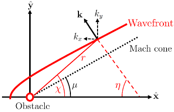
Figure 2: (color online) Schematic representation of a wavefront constant phase line (red solid line), traced by $\chi(\eta)$ and $r(\chi,\eta)$. The wavefronts are asymptotically parallel to the Mach cone (black dashed line) far from the obstacle (red circle).

V.1 Static reference frame, $\bar{u}\neq 0$ and $\bar{V}=0$

We perform finite-difference integration of the LL equation using the GPU-accelerated micromagnetic package MuMax3 Vansteenkiste et al. (2014). Although we report solutions of the nondimensional LL equation, Eq. (1), the parameters are consistent with Permalloy, e.g., saturation magnetization $M_{s}=790$ kA/m, exchange stiffness $A=10$ pJ/m³, and Gilbert damping $\alpha=0.01$. To compare with theory, we consider only local dipolar fields (zero thickness limit) by incorporating a negative perpendicular anisotropy constant $K_{u}=-\mu_{0}M_{s}^{2}/2$, where $\mu_{0}$ is the vacuum permeability. With these parameters, space is normalized to the exchange length $\lambda_{\mathrm{ex}}$ and time to $1/(\gamma\mu_{0}M_{s})$, where $\gamma$ is the gyromagnetic ratio. Typical values for these parameters are $\lambda_{\mathrm{ex}}=5$ nm, $1/(\gamma\mu_{0}M_{s})=36$ ps, and $\gamma=28$ GHz/T.

An impenetrable obstacle is introduced as a localized (hyper-Gaussian), perpendicular field that forces $\bar{n}=1$, i.e., the vacuum state, in a limited area Iacocca, Silva, and Hoefer (2017). In fact, a perpendicular field gradient acts as a potential body force on the fluid as shown in Eq. (5b). Alternatively, a magnetic defect or absence of magnetization also constitutes an impenetrable object. As an initial condition, we impose a SDW given by $(\bar{n},\bar{u}=0.6)$ with $0<\bar{n}<1$, and we guarantee its stability both by applying a homogeneous, perpendicular magnetic field that satisfies Eq. (6) and by defining a simulation domain of $L_{x}\times L_{y}=317\times 156$ spatial units that accommodates an exact number of SDW periods in the $\hat{\mathbf{x}}$ direction. The simulation is discretized into a mesh with $1024\times 512$ gridpoints and we implement periodic boundary conditions along the $\hat{\mathbf{x}}$ direction and open or free-spin conditions in the $\hat{\mathbf{y}}$ direction. The simulation is evolved to the time $t=112$. In order to prevent any nucleated structure from propagating through the periodic boundaries, we also implement a high damping region close to the edge of the simulation domain. Such an absorbing boundary does not compromise the stability of the initialized SDW. We emphasize that the choice of fluid velocity $\bar{u}=0.6$ was made on the basis of computational speed. Other fluid velocities give similar results.

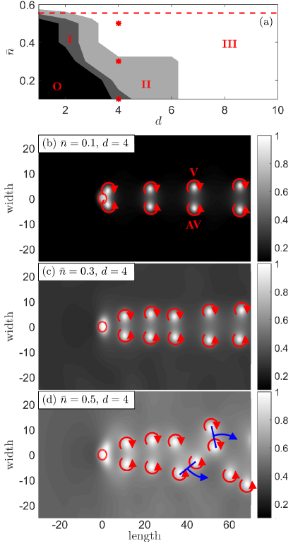
Figure 3: (color online) (a) Phase diagram for V-AV nucleation and dynamics in the static reference frame. Region O represents laminar flow while the gray regions I-II (III) denote ordered (irregular) V-AV pair nucleation. Snapshots of the longitudinal spin density, $n$, exemplify each region showing V-AV pairs in (b) parallel (region I), (c) unstable mode (region II), and (d) irregular dynamics (region III), with corresponding conditions indicated by red asterisks in (a). The red arrows represent the vortices’ circulation direction, with V and AV circulations indicated in (b). The blue lines and arrows schematically show the rotating trajectory of the V-V and AV-AV pairs in the irregular regime.

The observed nucleated nonlinear structures can be classified in the phase space spanned by the parameters $\bar{n}$ and $d$, shown in Fig. 3(a), swept in steps of $0.1$ and $1$, respectively. First, we note that laminar flow (region O) is lost as the diameter of the obstacle increases, even in the subsonic regime (below the dashed line), indicating that the fluid velocity locally develops supersonic speed as it is accelerated around the obstacle. We have verified this fact numerically. The gray regions represent ordered V-AV pair nucleation. For a relatively narrow parameter space (region I), the V-AV pairs translate parallel to each other carried by the underlying flow, as shown in Fig. 3(b). In region II, the parallel V-AV trains are unstable Nore, Brachet, and Fauve (1993) [Fig. 3(c)]. We note that the instability numerically observed for parallel V-AV pairs in BECs Nore, Brachet, and Fauve (1993) suggests that region I could eventually develop an instability for larger simulation domains and times. However, simulations in a domain twice as large $634\times 212$, evolved twice as long to $t=224$ did not show evidence of such an instability. Finally, region III denotes irregular V-AV nucleation, as shown in Fig. 3(d). Here, V-V and AV-AV rotation is observed, schematically shown in Fig. 3(d) by the blue lines defining the V-V and AV-AV axis and blue arrows denoting the rotation. In all the cases mentioned above, we observe that the separation between the V and AV in a pair increases as they translate away from the obstacle, similar to a Magnus force. This was also observed in additional simulations in which a single V-AV pair was nucleated by a field pulse. Such a single pair moves with a velocity greater than $|\mathbf{u}|$ and develops a velocity transverse to $\mathbf{u}$. This is in contrast to constant V-AV motion in a uniform magnetic background Papanicolaou and Spathis (1999). An in-depth study of V-AV motion on a textured background is worthy of future investigation, but it lies outside the scope of the present paper.

Micromagnetic simulations were performed also in the case in which a magnetic void with free spin boundary conditions serves as an obstacle. The resulting $\bar{n}$ vs $d$ phase space is shown in Fig. 4(a) and agrees qualitatively with the phase diagram obtained with a localized field [Fig. 3(a)]. We note that in this case, the instability of the V-AV pairs train develops into a sinous mode [Fig. 4(b)]. Furthermore, we observe a transition between region II and III, labeled region IV in Fig. 4(a), where we observe V-V and AV-AV nucleation reminiscent of von Kármán vortex streets numerically predicted and recently observed in BECs Sasaki, Suzuki, and Saito (2010); Kwon et al. (2016).

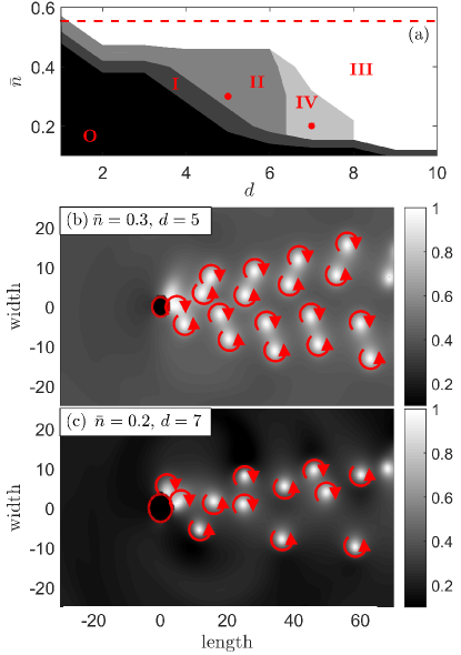
Figure 4: (color online) (a) Phase diagram for V-AV nucleation and dynamics in the static reference frame considering a magnetic defect as an obstacle. The black region represents laminar flow while the gray regions (white region) denotes ordered (irregular) V-AV pairs nucleation. Regions I and II qualitatively agree with the dynamics observed in Fig. 3. Here, region II exhibits a sinuous mode (b), in contrast to Fig. 3. Additionally, a von Kármán-like vortex street is observed in region IV (c). We do not show regions I and III as they are similar to Figs. 3b and 3c, respectively.

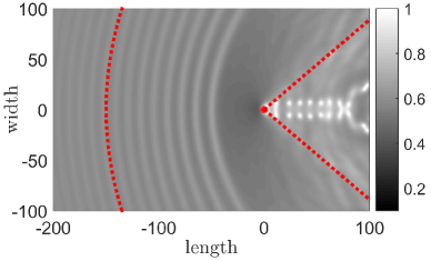
Figure 5: (color online) Snapshot of the longitudinal spin density, $n$, in the static reference frame at a supersonic condition $(\bar{n},\bar{u})=(0.6,0.6)$ and an obstacle of diameter $d=6$. The Mach cone calculated from Eq. (19a) and the wavefront calculated from Eq. (22) are shown by red dashed curves.

Irregular V-AV nucleation persists for supersonic conditions, when $M_{u}>1$ [above the red dashed line in Fig. 3(a)]. Additionally, in this regime we also observe a well-defined Mach cone and the nucleation of wavefronts (Fig. 5). As discussed in Sec. IV, the Mach angle and curves of constant phase corresponding to wavefronts are given in Eqs. (19a) and (22), which describe the numerical results to good accuracy, as shown by red dotted lines in Fig. 5. Whereas the Mach angle defines a static boundary i.e., the Mach cone, the wavefronts are dynamic due to vortex shedding and the concomitant change of flow conditions effected by our energy minimizing simulations. For this reason, the estimates of Eq. (20) are only valid for timescales shorter than the relaxation time imposed by damping. By fitting $\theta$ and a horizontal shift from the obstacle, the red dashed line outlining the wavefront in Fig. 5 is obtained. The wavelength $2\pi/|\mathbf{k}|=\lambda=19$ at $\eta=0$ is well-described by Eq. (20) and is found to be within the same order of magnitude as the numerically calculated wavefront wavelengths throughout the simulation evolution $\lambda_{\mathrm{sim}}=12.21\pm 2.1$. This agreement is possible due to the fact that the equations are effectively conservative for short timescales and the concepts used for BEC are approximately applicable.

V.2 Moving reference frame, $\bar{u}=0$ and $\bar{V}\neq 0$

In the moving reference frame, we use a pseudo-spectral method Hoefer and Sommacal (2012) to solve the nondimensionalized LL equation, Eq. (1). Here, the localized, perpendicular field moves with velocity $\bar{V}$ while the fluid velocity is zero. The simulation domain in this case has the same size as the simulations in the static reference frame but it is discretized into the coarser $256\times 128$ number of grid points by virtue of the accuracy of the pseudo-spectral method. We initialize the simulation with a homogeneous magnetization with $\bar{n}=h_{0}=0.7$, $\bar{u}=0$ and we use periodic boundary conditions along and across the thin film. We evolve the simulation to $t=2000$. The longer simulation time in this case reflects the slower dynamics in the moving reference frame. The value of the homogeneous perpendicular field bias magnitude, $h_{0}$, was chosen to minimize the strength of the localized perpendicular field needed to impose hydrodynamic vacuum.

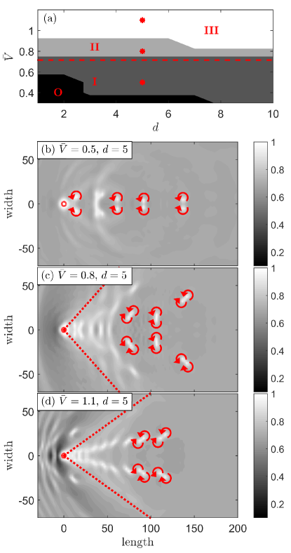
Figure 6: (color online) (a) Phase diagram for V-AV nucleation and dynamics in the moving reference frame. Region O represents laminar flow, where vortices are not nucleated. The gray regions I-II (region III) denote irregular (ordered) V-AV pair nucleation. Snapshots of the longitudinal spin density, $n$, show V-AV (b) annihilation (region I), (c) irregular dynamics (region II) and (d) ordered dynamics (region III) inside the Mach cone with conditions indicated by red asterisks in (a). The red arrows represent the vortices’ circulation direction.

The phase space for the nucleated nonlinear structures and dynamics as a function of $\bar{V}$ and $d$ are shown in Fig. 6(a), swept in steps of $0.1$ and $1$, respectively. As in Fig. 3(a), subsonic laminar flow (region O) is lost as the obstacle diameter increases. Regions I to III denote V-AV pair nucleation. In contrast to the static reference frame, the absence of an underlying fluid velocity in this case, $\bar{u}=0$, precludes significant vortex translation or Kelvin motion. Instead, the V-AV pairs are attracted to each other due to magnetic damping (energy dissipation) and subsequently annihilate, expelling spin waves. For this reason, the V-AV pairs nucleated at subsonic conditions (region I) are unstable and lead to an unevenly spaced V-AV train as well as irregular dynamics close to the obstacle [Fig. 6(b)]. At supersonic conditions, above the red dashed line in Fig. 6(a), a narrow phase space (region II) leads to irregular V-AV pairs inside the Mach cone, shown in Fig. 6(c) by red dashed lines calculated from Eq. (19b). Finally, in region III, the V-AV pairs become mostly ordered. In Fig. 6(d) we observe two V-AV pairs establishing an oblique path with respect to the obstacle. This is reminiscent of oblique solitons El, Gammal, and Kamchatnov (2006), but here the structure immediately breaks down into V-AV pairs.

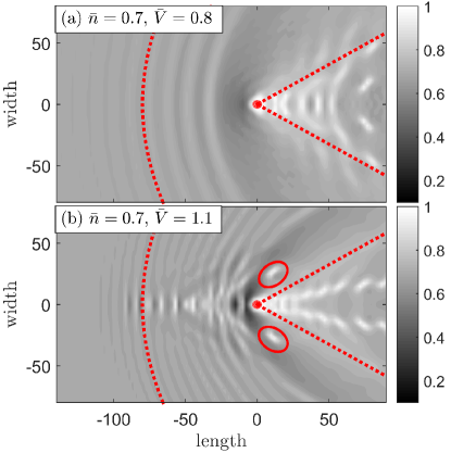
Figure 7: (color online) Snapshots of the longitudinal spin density, $n$, in the moving reference frame at supersonic conditions. The moving localized field has a diameter $d=5$. The Mach cone calculated from Eq. (19a) and the wavefront calculated from Eq. (21a) are shown by red dashed lines. Instabilities in the wavefronts lead to V-AV pairs, red circles.

As discussed above, a Mach cone and wavefronts are also established at supersonic conditions in the moving reference frame. These agree to good accuracy with Eqs. (19b) and (21), where the curves of constant phase for $\rm x$ and $\rm y$, analogous to Eq. (22), are determined as in Gladush et al., 2007. Figure 7 shows the comparison between theory and numerics. However, we observe instabilities in the wavefronts that develop for large obstacle velocities. This is shown in Fig. 7(a) and (b) for, respectively, velocities similar to and larger than the sonic curve. In particular, the short wavefronts in Fig. 7(b) are observed to break into V-AV pairs due to this instability (encircled in red) suggesting nonlinear effects. The study of such effects is beyond the scope of the current paper.

VI Conclusion

In summary, we demonstrate that nonlinear structures and V-AV complexes can be nucleated from an obstacle in a thin film planar ferromagnet. These observations are in qualitative agreement with structures nucleated in classical fluids and superfluids, providing further evidence for the hydrodynamic properties of thin film planar ferromagnets.

Both in the moving and static reference frames, we observe nucleation of V-AV pairs, as qualitatively expected for an unsteady wake formed behind an impenetrable obstacle. These V-AV pairs experience diverse dynamics and are nucleated as long as the system is out of equilibrium. In the static reference frame, we observe Kelvin motion, instability, and V-V, AV-AV rotation. In the moving reference frame, V-AV pairs are also nucleated but generally annihilate, forming an irregular pattern and spin waves. For supersonic conditions, a Mach cone and the formation of wavefronts are observed, as expected for superfluids. Good quantitative agreement is found between the numerically observed structures and theoretical results derived from the linearized, conservative, long-wave equations.

Although nonlinear structures and V-AV complexes are observed in both the static and moving reference frames, there are important differences in their dynamics. In particular, irregular V-AV dynamics are observed in supersonic conditions in the static reference frame, $\bar{u}>0$ and $\bar{V}=0$, and subsonic conditions in the moving reference frame, $\bar{u}=0$ and $\bar{V}>0$. This is due to the fact that the underlying flow, $\bar{u}\neq 0$, induces V-AV translation in contrast to the moving reference frame with $\bar{u}=0$. In other words, a topological texture is required to support ordered vortex structures. This suggests that for a fixed $\bar{u}>0$ the introduction of $\bar{V}\neq 0$ leads to irregularity in the subsonic regime. Additionally, the numerical observation of an apparently stable V-AV train propagating on the textured background $\bar{u}>0$ is to be contrasted with the unstable propagation of a train of counter-rotating vortices in a BEC. This intriguing ordered regime requires further analysis.

It is noteworthy that we explore a two-dimensional parameter space with a fixed $\bar{u}$ in the static reference frame and a fixed $\bar{n}$ in the moving reference frame, as opposed to the full three-dimensional parameter space where $\bar{n}$, $d$, and $\bar{u}$ or $\bar{V}$ are varied. However, we argue that the phase spaces shown in Fig. 3(a) and Fig. 6(a) represent general qualitative features of the full parameter space. The phase space can collapse to two dimensions, spanning $\mathrm{M}_{u}=\mathrm{M}_{u}(\bar{n},\bar{u})$ or $\mathrm{M}_{V}=\mathrm{M}_{V}(\bar{n},\bar{V})$ versus $d$. Micromagnetic simulations performed with several choices of $\bar{n}$ and $\bar{u}$ and $\bar{V}$ for, respectively, the static and moving reference frames, indeed return qualitatively similar dynamics for matching Mach numbers and obstacle diameters.

The above results show that V-AV complexes can be nucleated in a thin film ferromagnet with planar anisotropy following well-defined patterns analogous to superfluids and compressible fluids. Our observations are relevant for the stability of spin-density waves and the study of V-AV interactions with other nonlinear textures such as spin-density waves, other V-AV pairs, and wavefronts.