Income and wealth distribution of the richest Norwegian individuals: An inequality analysis

Abstract

Using the empirical data from the Norwegian tax office, we analyse the wealth and income of the richest individuals in Norway during the period 2010–2013. We find that both annual income and wealth level of the richest individuals are describable using the Pareto law. We find that the robust mean Pareto exponent over the four-year period to be $\approx 2.3$ for income and $\approx 1.5$ for wealth.

1 Introduction

Income and wealth inequalities are being closely examined in current economic, sociological and econophysical literature [1, 2, 3, 4, 5, 6, 7, 8, 9, 10, 11, 12, 13, 14, 15, 16, 17, 18, 19, 20, 21, 22, 23, 24, 25, 26, 27, 28]. The challenge is to accurately measure these inequalities.

The recent, widely-cited book on income and wealth inequalities by Piketty [1] concludes that income and wealth inequalities are different quantities and should be analyzed separately. Many authors have used the Pareto law to describe income or/and wealth inequalities [3, 4, 5, 6, 7, 8, 9, 10, 11, 12, 13, 14, 15, 16, 17, 18, 19, 20, 21, 22, 23, 24, 25, 26, 27, 28]. Piketty uses aggregated macro-variables to describe inequality, but these authors following the Pareto approach primarily use microdata, i.e., the wealth ranks of the richest individuals supplied by such periodicals as Forbes. In both kinds of analysis the quality of the empirical data is poor. Piketty’s empirical data, although reliable, are imperfect, and those used by other researchers are also far from perfect, because the only reliable source for such data is the tax office.

Since the publication of Vilfredo Pareto’s pioneering work on income distribution in the late nineteenth century many additional studies have been carried out to empirically verify the Pareto law for both individuals and households. These analyses were carried out for the United States [3, 4, 5, 6, 7, 8, 9, 10, 11], the European Union [6, 12, 11], the UK [3, 5, 7, 8, 13], Germany [3], Italy [14, 15], France [7], Switzerland [16], Sweden [8], Japan [17, 18, 19, 9, 20], Australia [14, 21], Canada [22], India [22, 23], Sri Lanka [22], Peru [16], Egypt [22], South Korea [24], Romania [25], Portugal [22], Poland [26, 6], and for the world as a whole [27, 28].

Here we use the Pareto law to analyze the income and wealth rank of the 100 richest individuals in Norway. Beginning in the nineteenth century, the tax office in Norway has compiled a yearly “Skattelister,” a list of the yearly income and wealth level of every citizen in Norway. Although access to the Skattelister has been extremely limited, the records of the 100 richest individuals are publicly available for the years 2010–2013. This allows a precise validation of the Pareto law for income and wealth distributions during those years [29]. Note that although current literature provides numerous occasions of this type of analysis, the Skattelister data we obtained from the Norwegian tax office makes our validation particularly reliable.

2 Pareto law

At the end of nineteenth century Vilfredo Pareto formulated his law by analyzing a huge amount of empirical data that described the income and wealth distributions using the PDF universal function, i.e. [16, 30, 12],

$$P(m)=\left\{\begin{array}[]{cc}\displaystyle\frac{\alpha}{m_{0}}\left(\frac{m_{0}}{m}\right)^{\alpha+1}&\mathrm{if}\quad m\geq m_{0}\\ 0&\mathrm{if}\quad m<m_{0}\end{array}\right.,$$ (1)

which defines the Pareto law [30]. The $m_{0}$ value is the lowest value of variable $m$ and $\alpha$ is the Pareto exponent. By definition we choose the strongest Pareto law [30] for $\alpha=3/2$.

Empirical studies indicate (i) that the mean value of the Pareto exponent is close to $2$, and (ii) that the Pareto law is valid for large values of income and wealth [22]. For other values of income and wealth such laws as Gibrat’s rule of proportionate growth [22] are valid. Thus the studies in Section 1 refer to the weak Pareto law that holds in the limit $m\gg m_{0}$. We will show that the mean value of the Pareto exponent for the richest Norwegians is close to $2$ for income and to $3/2$ for wealth.

To analyse the empirical data it is better to use the more robust (global) empirical complementary cumulative distribution function (CCDF) rather than the (local) Eq. (1). From Eq. (1) the CCDF can be written

$$\Pi(m)=(m/m_{0})^{-\alpha},\quad\textrm{for }m\geq m_{0}.$$ (2)

A well-known feature of Eq. 1 is the divergence of its moments of an order greater than or equal to $\alpha$. This means that we should apply quantiles (which are always finite [31]) instead of moments. For example, we use the median instead of the mean value. In any case, the moment estimates are always finite and can be calculated directly from the empirical data [12].

3 Results and concluding remarks

The annual rankings of income and wealth of Norwegian citizens for the years 2010–2013 [29] are of the 100 wealthiest people in Norway as well as in each region (fylke) of Norway. Note that income and wealth ranking lists are reported independently. Someone listed in the income ranking is not listed in the wealth ranking and vice versa. Unlike those in, for example, Forbes, the data supplied by the Norwegian tax office are not estimates and are of the highest quality.

Figure 1 shows log-log plots of the wealth and income rankings for the Hedmark region and Norway as a whole for the year 2013. The slopes of these lines are equal to $-\alpha_{\textrm{rank}}$ and were calculated using a fitting routine. The inverse of $\alpha_{\textrm{rank}}$ gives the Pareto exponent $\alpha$.

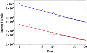
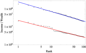
Figure 1: Ranks of income (bottom plots) and wealth (top plots) of the richest individuals in Norway (left panel) and Hedmark region (right panel). Solid lines were obtained by fitting straight lines (in the log-log scale) to empirical data (dots) for year 2013.

Table 1 shows the Pareto exponents for each region of Norway and for all of Norway for the years 2010–2013. The error bars of the Pareto exponents fall within the range 0.01–0.13.

Table 1: Pareto exponents for each region of Norway and all of Norway the for years 2010–2013. The errors bars of Pareto exponents fall within the range $0.01-0.13$.

Region/year	2010		2011		2012		2013
	income	wealth	income	wealth	income	wealth	income	wealth
Akershus	$2.45$	1.14	3.00	1.21	2.34	1.23	2.45	1.43
Aust-Agder	$2.22$	1.20	2.19	1.13	1.70	1.14	1.58	1.16
Buskerud	$2.11$	1.43	1.63	1.26	1.75	1.25	2.11	1.50
Finnmark	$2.90$	1.63	2.69	1.63	2.94	1.61	2.90	1.81
Hedmark	$2.12$	1.61	2.14	1.67	1.14	1.66	2.12	1.86
Hordaland	$2.13$	1.25	2.13	1.18	1.78	1.23	1.69	1.13
Møre Og Romsdal	$2.42$	1.46	1.54	1.54	2.19	1.94	2.42	1.62
Nordland	$2.15$	2.08	2.59	1.84	1.88	1.75	2.47	2.25
Nord-Trøndelag	$2.93$	2.46	2.30	2.26	2.04	1.93	2.95	2.05
Oppland	$2.26$	1.88	2.53	1.85	2.12	1.83	2.47	1.92
Oslo	1.53	1.26	1.90	1.37	2.55	1.40	2.05	1.44
Østfold	$1.90$	1.81	2.12	2.08	2.37	2.19	1.60	1.95
Rogaland	$1.82$	1.65	2.32	1.57	2.28	1.54	2.58	1.54
Sogn Og Fjordane	$2.55$	1.44	2.19	1.36	2.50	1.36	2.05	1.36
Sør Trøndelag	$1.72$	1.75	1.51	1.55	1.79	1.42	2.01	1.49
Telemark	$2.87$	1.35	2.54	1.35	2.39	1.44	2.60	1.47
Troms	$2.11$	1.45	1.23	1.43	2.60	1.54	2.41	1.00
Vest-Agder	2.11	1.02	2.22	1.03	2.11	0.97	2.09	1.48
Vestfold	2.22	1.34	2.23	1.55	2.37	1.54	2.52	1.67
NORWAY	1.69	1.37	1.77	1.35	2.01	1.37	1.72	1.55
Mean (regions)	2.23	1.54	2.16	1.52	2.15	1.52	2.27	1.59
Dispersion (regions)	0.37	0.34	0.43	0.31	0.40	0.30	0.38	0.32

The mean Pareto exponent $\alpha$ over a four-year period for Norway is $2.3\pm 0.4$ for income and $1.5\pm 0.3$ for wealth. Note that the Pareto exponent for income is significantly larger than the Pareto exponent for wealth. This is the most reliable result thus far obtained for income and wealth analysis [3, 4, 5, 6, 7, 8, 9, 10, 11, 12, 13, 14, 15, 16, 17, 18, 19, 20, 21, 22, 23, 24, 25, 26, 27, 28]. In addition, the Pareto exponents for income fluctuate in time more than Pareto exponents for wealth. This means that wealth inequality is more difficult to change than income inequality. Note that the results obtained thus far by authors not using data supplied by tax authorities are unsystematic and approximate.

Using our comparative analysis we find that for separate regions in Norway the Pareto exponents for wealth are almost always smaller than the corresponding Pareto exponents for income. This means that wealth inequality is higher than income inequality, i.e., the lower the Pareto exponent, the higher the inequality. This is because income has no accumulation effect across the generations that acts according to the preferential choice rule, “the rich become richer.” Income inequality is strongly affected by access to skills and higher education and is lowered by taxes on income, but wealth accumulation is a long-term process and is less burdened by taxes, i.e., a cadastral tax or inheritance tax does not significantly reduce wealth inequality (see [1]). Although one possible solution to this situation would be to introduce an annual tax on wealth, social and political factors make this change difficult [1].

Using high quality empirical data from the Norwegian tax office, we have analyzed income and wealth of the richest Norwegian individuals. We find that income and wealth inequality should be analyzed separately because they are driven by different factors [1]. In addition, we confirm that the distribution of top income and wealth is subject to the Pareto law.

We are aware that the analysis of income and wealth is a research area for which much has yet to be accomplished. We hope that our paper contributes some insight into the topic from a physicist’s point of view. The proposed approach is a link between economics and econophysics and shows that the economic models describing the relationship between income and wealth can be supported by modelling based on methods used by physicists.

References

- Piketty [2014] T. Piketty, Capital in the Twenty-First Century (The Belknap Press of Harvard University Press, Cambridge, 2014).
- by A. B. Atkinson and Bourguignon [2015] E. by A. B. Atkinson and F. Bourguignon, Handbook of Income Distribution (Elsevier B.V., 2015).
- Clementi and Gallegati [2005a] F. Clementi and M. Gallegati, in Econophysics of Wealth Distributions, edited by A. Chatterjee, B. K. Chakrabarti, and S. Yarlagadda (Springer, Italy, 2005) pp. 3–14.
- Clementi et al. [2009] F. Clementi, M. Gallegati, and G. Kaniadakis, Journal of Statistical Mechanics , P02037 (2009).
- Drăgulescu and Yakovenko [2001] A. Drăgulescu and V. M. Yakovenko, Physica A 299, 213 (2001).
- Jagielski et al. [2012] M. Jagielski, R. Kutner, and M. Pȩczkowski, Acta Phys. Pol. A 121, B47 (2012).
- Levy [1998] S. Levy, Recent Work, Finance (1998), http://escholarship.org/uc/item/5zf0f3tg.
- Levy [2003] M. Levy, Journal of Economic Theory 110, 42 (2003).
- Nirei and Souma [2007] M. Nirei and W. Souma, Review of Income and Wealth 53, 440 (2007).
- Yakovenko and Rosser [2009] V. M. Yakovenko and J. B. Rosser, Reviews of Modern Physics 81, 1703 (2009).
- Jagielski et al. [2015] M. Jagielski, R. Duczmal, and R. Kutner, Physica A 433, 36 (2015).
- Jagielski and Kutner [2013] M. Jagielski and R. Kutner, Physica A 392, 2130 (2013).
- Scafetta et al. [2004] N. Scafetta, S. Picozzi, and B. J. West, Physica D 193, 338 (2004).
- Clementi et al. [2006] F. Clementi, T. D. Matteo, and M. Gallegati, Physica A 370, 49 (2006).
- Clementi and Gallegati [2005b] F. Clementi and M. Gallegati, Physica A 350, 427 (2005b).
- Pareto [1897] V. Pareto, Cours d’économie politique (L’Université de Lausanne, 1897).
- Aoyama et al. [2003] H. Aoyama, W. Souma, and Y. Fujiwara, Physica A 324, 352 (2003).
- Aoyama et al. [2000] H. Aoyama, W. Souma, Y. Nagahara, M. P. Okazaki, H. Takayasu, and M. Takayasu, Fractals 8, 293 (2000).
- Fujiwara et al. [2003] Y. Fujiwara, W. Souma, H. Aoyama, T. Kaizoji, and M. Aoki, Physica A 321, 598 (2003).
- Souma [2001] W. Souma, Fractals 9, 463 (2001).
- Matteo et al. [2004] T. D. Matteo, T. Aste, and S. T. Hyde, in The Physics of Complex Systems (New Advances and Perspectives), edited by F. Mallamace and H. E. Stanley (IOS Press, Amsterdam, 2004) pp. 435–442.
- Richmond et al. [2006] P. Richmond, S. Hutzler, R. Coelho, and P. Repetowicz, in Econophysics & Sociophysics: Trends & Perspectives, edited by B. Chakrabarti, A. Chakraborti, and A. Chatterjee (WILEY-VCH, Weinheim, 2006) pp. 129–158.
- Sinha [2006] S. Sinha, Physica A 359, 555 (2006).
- Kim and Yoon [2004] K. Kim and S. M. Yoon, “Power law distributions in korean household incomes,” (2004), unpublished paper at: http://arxiv.org/abs/cond-mat/0403161.
- Derzsy et al. [2012] N. Derzsy, Z. Néda, and M. A. Santos, Physica A 391, 5611 (2012).
- Jagielski and Kutner [2010] M. Jagielski and R. Kutner, Acta Physica Polonica A 117, 615 (2010).
- Klass et al. [2007] O. S. Klass, O. Biham, M. Levy, O. Malcai, and S. Solomon, The European Physical Journal B 55, 143 (2007).
- Levy and Solomon [1997] M. Levy and S. Solomon, Physica A 242, 90 (1997).
- NTO [2015] “Skattelister,” Norwegian Tax Office (2015), http://www.dn.no/skattelister/.
- Mandelbrot [1960] B. Mandelbrot, International Economic Review 1, 79 (1960).
- Hyndman and Fan [1996] R. J. Hyndman and Y. Fan, The American Statistician 50, 361 (1996).