Bound states of a light atom and two heavy dipoles in two dimensions

Abstract

We study a three-body system, formed by a light particle and two identical heavy dipoles, in two dimensions in the Born-Oppenheimer approximation. We present the analytic light-particle wave function resulting from an attractive zero-range potential between the light and each of the heavy particles. It expresses the large-distance universal properties which must be reproduced by all realistic short-range interactions. We calculate the three-body spectrum for zero heavy-heavy interaction as a function of light to heavy mass ratio. We discuss the relatively small deviations from Coulomb estimates and the degeneracies related to radial nodes and angular momentum quantum numbers. We include a repulsive dipole-dipole interaction and investigate the three-body solutions as functions of strength and dipole direction. Avoided crossings occur between levels localized in the emerging small and large-distance minima, respectively. The characteristic exchange of properties such as mean square radii are calculated. Simulation of quantum information transfer is suggested. For large heavy-heavy particle repulsion all bound states have disappeared into the continuum. The corresponding critical strength is inversely proportional to the square of the mass ratio, far from the linear dependence from the Landau criterion.

I Introduction

The experimental realization of ultracold atomic traps with the further control of the interaction between the atoms using the Feshbach resonance technique pethick ; BloRMP2008 ; ChiRMP2010 provided an unprecedented playground to study few-body correlations NiePR2001 ; BraPR2006 ; BluRPP2012 ; FreFBS2011 that started long ago uniquely as a theoretical study in the nuclear context PhiNPA1968 ; CoePRC1970 ; TjoPL1975 ; EfiPL1970 . More specifically, the tunability of the two-body interaction turned into a fact the prediction made by Efimov that a system compounded by three identical bosons presents an infinite number of bound states when the energy of the two-boson subsystem tends to zero EfiPL1970 . This interesting phenomenon occurs exclusively in three dimensions NiePR2001 as a consequence of the collapse of the three-body scale ThoPR1935 .

The first proposal about how to use magnetic fields in order to confine cold neutral atoms was made by Pritchard in 1983 PriPRL83 and its experimental observation was made two years later by Migdall MigPRL85 . Almost ten years after the first neutral atoms have been trapped, the question of dimensionality started to be explored in experiments SchAPB95 . Many aspects of the physics may change drastically when the system passes from three to two dimensions WerPRA2012 ; BelFBS2015 ; YamJPB2015 . Two pertinent examples can be cited here. The first one is the possibility to have an inherent attraction for zero orbital angular momentum that automatically appears from the kinetic energy. The consequence is that any infinitesimal attraction binds the system (in three dimensions the centrifugal barrier is always repulsive or null). The second example is related to the Efimov effect cited in the previous paragraph. In two dimensions the Thomas collapse is absent and no new scale should be added to the system at the universal regime: a two-body scale (the two-body energy, $E_{2}$, for example) defines completely the three-body observables, e.g. for three identical bosons there are only the ground and first excited states with energies satisfying, respectively, the relations $E_{3}^{(0)}=16.52E_{2}$ and $E_{3}^{(1)}=1.27E_{2}$ BruPRA1979 . The universal regime is accessed when the size of the system (a good quantity to describe it can be the two-body scattering length, $a$) is much greater than the range of the potential, $r_{0}$. In this regime, the observables do not depend on the details of the short-range potential.

The proportionality relations between $E_{2}$ and $E_{3}$ immediately shows that the infinite number of three-body bound states when $E_{2}=0$ is no longer possible in the bidimensional situation LimPRB1980 ; AdhPRA1988 . However, we can imagine a favorable design to generate more than two three-body bound states. It was derived long ago that for an asymmetric system $AAB$ formed by two identical bosons with mass $m_{A}$ and a different atom with mass $m_{B}$, it is possible to generate as many states as desired decreasing the ratio $m_{B}/m_{A}$. The physical interpretation is that the effective potential becomes more attractive as the light atom can be easily exchanged by the heavy ones LimZPA1980 . The possibility to increase the attraction just by changing the mass ratio between the atoms creates an interesting situation: for any repulsion between the atoms of the heavy pair, we may always set a mass ratio in order to have a three-atom bound state.

There is still another interesting result associated with the combination of both interactions: the sum of the effective and repulsive potentials creates a barrier separating two minima each of them supporting bound states with proper tuning. The related tunneling can be identified by the avoided crossing behavior of the energy spectrum. The impressive development of the experimental techniques may then allow control over the localization of the wave function, and in turn provide a laboratory to simulate transfer of quantum information CirPRL1995 ; EckPRA2002 ; StrPRA2008 ; SodNJP2009 ; LadNature2010 .

The constant experimental advances of techniques involving ultracold atomic traps in the last ten years produced a remarkable ability to control the quantum properties of single atoms in an optical lattice BakNature2008 ; WeiNature2011 . More recently, the study of dipoles became a hot topic in cold gases BarPR2008 ; LahRPP2009 ; KifPRL2013 ; HanPS2015 with a variety of experiments producing traps of mixed-atoms and dipole molecules NiScience2008 ; TakPRL2014 ; MolPRL2014 ; ParPRL2015 ; GuoPRL2016 . These long-range interactions may be controlled by changing the magnetic field or changing individually the magnetic moments of the atoms. The dipole interaction can be made attractive or repulsive depending on the orientation of the moments relative to their motion. The short-range interactions may be suppressed by using the Feshbach resonance to tune an infinity scattering length, and thereby producing a pure dipole-dipole interacting two-body system.

The paper is organized as follows. In section II we show briefly the formalism used to calculate in two dimensions (2D) a three-body system in the Born-Oppenheimer (BO) approximation formed by two identical heavy dipoles and one atom. We fix the directions of the dipoles in order to generate a repulsive or zero interaction between them. The atom-dipole interaction is assumed to be of very short range approximated by a zero-range interaction. We then derive the analytical form of the light-atom wave function in the configuration space which can be used as input to parametrize more realistic calculations. In section III we discuss the solutions for vanishing dipole interaction as function of the mass ratio. In section IV we investigate the solutions for finite dipole interaction. We specially focus on strengths around degeneracy of states localized in inner and outer minima, and finally we derive critical dipole-dipole strengths for stability of the three-body system. A summary and conclusions are presented in section V.

II Formalism

In this section we show the formalism used to solve the three-body system formed by two heavy dipoles with masses $m_{A}$ and an atom with mass $m_{B}$. We follow closely the theory from Ref. BelJPB2013 repeating part of it in order to be selfcontained. We will consider the system depicted schematically in Fig. 1. The Hamiltonian is given by

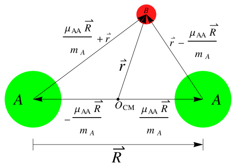
Figure 1: Three-body system formed by two identical dipoles with mass $m_{A}$, $\mu_{AA}=m_{A}/2$, and an atom with mass $m_{B}$. We are considering the Born-Oppenheimer validity range where $m_{B}/m_{A}\ll 1$.

$$H = -\frac{\hbar^{2}}{2\mu_{AA}}\nabla^{2}_{R}-\frac{\hbar^{2}}{2\mu_{B,AA}}\nabla^{2}_{r}+V_{B}(\vec{R})$$ (1)

$$+ V_{A}(\vec{r}-\frac{\mu_{AA}}{m_{A}}\vec{R})+V_{A}(\vec{r}+\frac{\mu_{AA}}{m_{A}}\vec{R}),$$

where the reduced masses are given by $\mu_{AA}=m_{A}/2$ and $\mu_{B,AA}=2m_{A}m_{B}/\left(2m_{A}+m_{B}\right)$. Here we are using an odd-man-out notation that is $V_{A}$ and $V_{B}$ denote, respectively, the $AB$ (atom/dipole) and $AA$ (dipole/dipole) two-body interactions. Note that we work with relative coordinates after having removed the three-body center-of-mass motion.

Let us consider here that $m_{A}\gg m_{B}$. Due to this severe mass asymmetry we may consider the dipoles stationary when we solve the problem of the atom $B$. The total wave function may be written as a product of the wave functions of the fast atom, $\psi$, and slow dipoles, $\phi$, as $\Psi(\vec{r},\vec{R})=\psi(\vec{r},\vec{R})\phi(\vec{R})$, where the separation vector of the dipoles, $\vec{R}$, enters in $\psi$ only as a parameter. It is worth mentioning here that the total wave function is symmetric under the interchange of the heavy dipoles. As the interaction is not dependent on the spin, the formalism developed here may be suitable to describe a three-body system formed by bosonic or antiparallel fermionic dipoles.

The action of the Laplace operator, $\nabla_{R}^{2}$, on $\Psi$ in the Schroedinger equation is to lowest order approximated by $\nabla_{R}^{2}\phi(\vec{R})\psi(\vec{r},\vec{R})\approx\psi(\vec{r},\vec{R})\nabla_{R}^{2}\phi(\vec{R})$. Two other terms, $\phi(\vec{R})\nabla_{R}^{2}\psi(\vec{r},\vec{R})$ and $2\nabla_{R}\psi(\vec{r},\vec{R})\cdot\nabla_{R}\phi(\vec{R})$, also appear but usually they are much smaller and we neglect them in the present paper. We are then able to write independent equations for the heavy and light subsystems as

$$\left[-\frac{\hbar^{2}}{2\mu_{B,AA}}\nabla^{2}_{r}+V_{A}(\vec{r}-\frac{\mu_{AA}}{m_{A}}\vec{R})\right.$$

$$+\left.V_{A}(\vec{r}+\frac{\mu_{AA}}{m_{A}}\vec{R})\right]\psi(\vec{r},\vec{R})=\epsilon(R)\psi(\vec{r},\vec{R}),$$ (2)

$$\left[-\frac{\hbar^{2}}{2\mu_{AA}}\nabla^{2}_{R}+V_{B}(\vec{R})+\epsilon(R)\right]\phi(\vec{R})=E_{3}\phi(\vec{R}).$$ (3)

Note that the eigenvalue of Eq. (2), $\epsilon(R)$, depends on the relative position of the heavy dipoles, $R$, and enters as an effective potential in Eq. (3). The eigenvalue of this heavy dipoles equation returns the three-body binding energy, $E_{3}$.

II.1 Light-particle equation

The form of $\epsilon(R)$ was firstly derived in Refs. LimZPA1980 for two different Yamaguchi form factors. Further, in Ref. BelJPB2013 , this effective potential was calculated for a zero-range potential. It results from a solution of a transcendental equation given by

$$\ln\left[\frac{|\epsilon(R)|}{|E_{2}|}\right]=2K_{0}\left(\sqrt{\frac{2\mu_{B,AA}|\epsilon(R)|}{\hbar^{2}}}R\right),$$ (4)

where $K_{0}$ is the zero order modified Bessel function of the second kind. Solving this equation for $\epsilon(R)$ we see that the attraction increases when the mass ratio $m_{B}/m_{A}$ is decreased, as the light atom, which generates the effective attraction, can be more easily exchanged between the dipoles. This potential as well as the wave function in momentum space, $\psi(\vec{p},\vec{R})$ ($\vec{p}$ is the momentum canonically conjugate to $\vec{r}$), appeared in Ref. BelJPB2013 . The Fourier transform of $\psi(\vec{p},\vec{R})$ can be analytically calculated such that in coordinate space the light-atom wave function is given by:

$$\psi(\vec{r},\vec{R}) = -\frac{\mu_{B,AA}}{\hbar^{2}\pi}\left[K_{0}\left(\sqrt{\frac{2\mu_{B,AA}|\epsilon(R)|}{\hbar^{2}}}\rvert\vec{r}+\frac{\mu_{AA}}{m_{A}}\vec{R}\rvert\right)\right.$$ (5)

$$+ \left.K_{0}\left(\sqrt{\frac{2\mu_{B,AA}|\epsilon(R)|}{\hbar^{2}}}\rvert\vec{r}-\frac{\mu_{AA}}{m_{A}}\vec{R}\rvert\right)\right].$$

The atom-dipole binding energy, $E_{2}$, for a renormalized zero-range interaction enters as an input in the effective potential, $\epsilon(R)$, see Eq. (4). The form of the wave function given in Eq. (5) can be used to parametrize the light-heavy large-distance tail of the wave function of any potential satisfying the Born-Oppenheimer validity condition.

II.2 Heavy particles equation

In the next section we solve Eq. (3) numerically. Firstly, we change variables based on the small distance behavior of the effective potential. Note that for small distances, the effective potential is given by BelJPB2013

$$\epsilon(R)\rightarrow-\frac{2e^{-\gamma}|E_{2}|}{\sqrt{\frac{2\mu_{B,AA}|E_{2}|}{\hbar^{2}}}}\frac{1}{R}\ \ {\rm for}\ \ \sqrt{\frac{2\mu_{B,AA}|E_{2}|}{\hbar^{2}}}R\leq 1.15,$$ (6)

where $\gamma=0.5772$ is Euler’s constant. This Coulomb-like short-range behavior forces the system to act like a hydrogen atom with an effective squared charge given by

$$\mathcal{Q}_{\rm{eff}}^{2}=2\sqrt{\frac{\hbar^{2}}{2\mu_{B,AA}|E_{2}|}}e^{-\gamma}|E_{2}|,$$ (7)

and the corresponding modified Bohr radius

$$a_{0} = \frac{\hbar^{2}}{\mu_{AA}\mathcal{Q}_{\rm{eff}}^{2}}.$$ (8)

We can then rewrite Eq. (3), after making the change of variable from $R$ to $x$, that is $R=\left(a_{0}/2\right)x$, as

$$\left[\frac{\partial^{2}}{\partial x^{2}}-\frac{(l^{2}-1/4)}{x^{2}}\right]\chi(x)+\frac{a_{0}}{2\mathcal{Q}_{\rm{eff}}^{2}}\left[\epsilon(x)-V_{B}(x)\right]\chi(x)$$

$$=-\frac{a_{0}}{2\mathcal{Q}_{\rm{eff}}^{2}}E_{3}\chi(x),$$ (9)

where $\chi(x)=\sqrt{R}\phi(R)$, $V_{B}$ is the heavy-heavy particle potential, and the non-negative integer, $l$, is the angular momentum quantum number in two dimensions arising from the kinetic energy operator in spherical coordinates. It is worth noting here that Eq. (9) shows an important difference when considering three-dimensional (3D) or 2D systems, namely, for $l=0$ we have here an attractive centrifugal barrier, while in 3D the barrier is always repulsive or null.

III The three-body Born-Oppenheimer structure

We shall first discuss the Born-Oppenheimer wave function for a fixed distance between the two heavy particles. In the next subsection we present the basic three-body spectra for vanishing heavy-heavy particle potential.

III.1 Light particle wave function

The short-range potential between light and heavy particles is approximated by a zero-range interaction. This allows an analytic solution with the wave function in coordinate space explicitly given in Eq. (5). Rewriting the arguments in the Bessel function and using $\mu_{AA}=m_{A}/2$, we get

$$\psi(\vec{r},\vec{R}) = -\frac{\mu_{B,AA}}{\hbar^{2}\pi}\left[K_{0}(\zeta_{+})+K_{0}(\zeta_{-})\right]\;,$$ (10)

where the wave function is seen to be a function of two coordinates and one scale parameter $b$, that is

$$\zeta_{\pm} = \sqrt{b\left(\frac{r^{2}}{R^{2}}+\frac{1}{4}\pm\frac{r}{R}\cos(\theta_{rR})\right)}\;,$$ (11)

$$b = \frac{2\mu_{B,AA}R^{2}|\epsilon(R)|}{\hbar^{2}}.$$ (12)

Thus, the dimensionless combination in $b$ of energy, reduced mass and heavy-heavy distance determines this wave function completely together with the relative size, $r/R$, and the direction, $\cos(\theta_{rR})$, between the two relative coordinates, $\vec{r}$ and $\vec{R}$, see Fig. 1.

The wave function $\psi$ is symmetric around $\cos(\theta_{rR})=0$. The Bessel function has a logarithmic divergence when its argument aproaches zero, which in the present case occurs when $R=2r$ and $\cos(\theta_{rR})=\pm 1$. This is precisely when the light particle is on top of one of the heavy particles. For the employed short-range attraction this is not a surprise as the probability is largest in such a situation, as seen in Fig. 2. The two surfaces for different $b$ shows how the peak increases around the heavy particles as the two-body binding energy or heavy-heavy particle distance increases. The light particle becomes in both cases increasingly localized around one of the heavy particles, the effect of increasing $b$ is to make the wave function flatter.

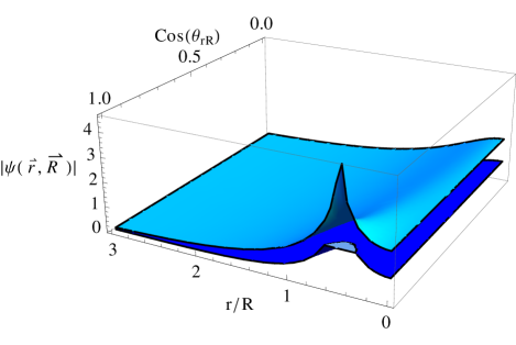
Figure 2: The wave function in Eq. (10) as a function of the relative size, $r/R$, and the direction, $\cos(\theta_{rR})$, between the two relative coordinates, $\vec{r}$ and $\vec{R}$, see Fig. 1. The upper and lower surfaces are, respectively, results for $b=1$ and $4$. The constant in front of Eq. (10) is fixed as $\mu_{B,AA}/(\hbar^{2}\pi)=1$.

The properties seen in Eq. (10) and illustrated in Fig. 2 reflect the genuine universal behavior for any short-range interaction in the Born-Oppenheimer approximation, provided the distances between light and heavy particles are much larger than the range of the respective potentials. This analytic form of the wave function can then be used as a boundary condition or to parametrize the tail of a general wave function.

III.2 Heavy particle motion

We now turn to the three-body bound-state properties obtained from Eq. (9). Initially, we consider noninteracting two heavy particles, $V_{B}=0$. The solutions are completely determined from the two-body energy, $E_{2}$, as functions of mass ratio, $m_{B}/m_{A}$, and angular momentum $l$. From Eq. (6), one can see that the effective potential for small distances behaves like a Coulomb potential. It can be rewritten in the new variables as

$$\epsilon(x)\rightarrow-|E_{2}|\left(\frac{\mu_{AA}}{\mu_{B,AA}}\right)\frac{4e^{-2\gamma}}{x}\ \ {\rm for}\ \left(\frac{\mu_{B,AA}}{\mu_{AA}}\right)x\leq 1.29.$$ (13)

The corresponding energy solutions, are given analytically by SaPRA2016

$$\frac{|E_{3}^{(C)}|}{|E_{2}|}=-\frac{1}{2(n+l-\frac{1}{2})^{2}}\left(\frac{\mu_{AA}}{\mu_{B,AA}}\right)2e^{-2\gamma},$$ (14)

where we inserted the effective charge from Eq. (7). The quantum numbers, $n$ and $l$, are both non-negative integers. The approximation in Eq. (14) contains the usual Coulomb degeneracy, where only the non-negative integer combinations, $n+l$, determine the energies. The mass dependence as well as the two-body interaction strength, $E_{2}$, are very trivial in this approximation.

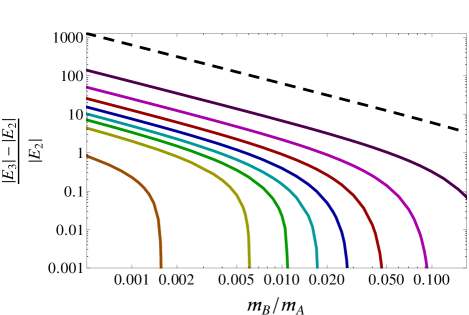
Figure 3: Three-body energy, $E_{3}$, with respect to the two-body threshold, $E_{2}$, as a function of the mass ratio of the atom ($m_{B}$) and the heavy dipoles ($m_{A}$) for orbital angular momenta ($l=0$). The dipole-dipole interaction, $V_{B}$, is zero. The dashed line is the ground state and the lines below it are, in sequence, results for the following excited states. The first and second of these excited $l=0$ states coincide within the line thickness with the ground states for $l=1$ as and $l=2$, respectively.

In Figure 3 we show the lowest three-body energies calculated numerically from Eq. (9) for $V_{B}=0$ as function of the mass ratio $m_{B}/m_{A}$. Each energy decreases with increasing $m_{B}/m_{A}$ as predicted by Eq. (14), and eventually reaches the continuum at individual threshold values. The number of bound states is correspondingly reduced with $m_{B}/m_{A}$ as also known in general from BelJPB2013 . The threshold behavior of both energy and structure is discussed in some details in SaPRA2016 .

The results for higher values of $l$ are almost indistinguishable within the thickness of the curves, except that the largest binding energy moves towards the next excited state for each unit of $l$. This is precisely the Coulomb degeneracy in two spatial dimensions as contained in Eq. (14). The ground state has $(n,l)=(0,0)$, the first doubly degenerate excited energy has $(n,l)=(1,0),(0,1)$, and the second $(n,l)=(2,0),(1,1),(0,2)$, etc. Thus, the number of bound states also decreases with $l$.

This degeneracy is quantified in Table 1 where our numerical results are compared with the analytic ones given by Eq. (14) for $l=0$ and $m_{B}/m_{A}=0.02$. As mentioned above the same numbers appear in comparison for larger $l$-values. We notice that the ratio of the numerically computed binding and the Coulomb values are $1.02$, $1.19$, $1.48$, and $1.96$ for increasing excitation energy, respectively. The principal reason is that Eq. (14) only is the lowest order in an expansion for small $x$, see BelJPB2013 . The next two terms contribute although varying only weakly with $x$, that is, the first is simply a constant and the second correction term is logarithmic in $x$. They both provide larger binding energy.

Table 1: Results for several states of the three-body energy in units of $E_{2}$ considering the BO approximation, $|E_{3}|/|E_{2}|$, and the exact hydrogen-atom calculation, $|E_{3}^{(C)}|/|E_{2}|$, for $l=0$. The mass ratio is fixed to $m_{B}/m_{A}=0.02$.

State	$|E_{3}|/|E_{2}|$	$|E_{3}^{(C)}|/|E_{2}|$	$(|E_{3}|-|E_{3}^{(C)}|)/|E_{2}|$
Ground	32.42	31.83	0.59
First	4.19	3.53	0.66
Second	1.88	1.27	0.61
Third	1.26	0.64	0.62

We emphasize that this discussion would be less and less relevant for excited states approaching the thresholds for binding. Then the deviations from the Coulomb estimate would arise from the extension of the states into a region with strongly deviating Coulomb potential. This happens by increasing excitation energy, increasing mass ratio, and increasing angular momentum.

IV Heavy particle motion with additional interaction

In this section we investigate the three-body solutions with an explicit heavy-heavy potential included on top of the Born-Oppenheimer potential $\epsilon(R)$ arising from the zero-range light-heavy potential. This heavy-heavy potential could in principle be of any form and strength; for example, extremely short- or long-range potentials. We shall here discuss only the realistic dipole-dipole potential of intermediate range. First we present the general analytic and numerical properties and in the last subsection we discuss the necessary critical strength to reach instability.

IV.1 Dipole-dipole interaction

Generically, for two dipoles, $m_{1}$ and $m_{2}$, connected by a vector $\vec{R}$, the dipole interaction is given by HanPS2015

$$V_{B}(\vec{R})=C\left[\frac{\vec{m}_{1}\cdot\vec{m}_{2}}{R^{3}}-\frac{3(\vec{m}_{1}\cdot\vec{R})(\vec{m}_{2}\cdot\vec{R})}{R^{5}}\right],$$ (15)

where $C=\mu_{0}/4\pi$ and $C=1/4\pi\epsilon_{0}$ for magnetic and electric dipoles, respectively (note that in Gaussian units the first and second constants should be replaced, respectively, by $C=1/c^{2}$ and $C=1$, where $c$ is the speed of light). Here $\mu_{0}$ is the vacuum permeability and $\epsilon_{0}$ the vacuum permittivity. For two identical dipoles in the $xy$-plane with dipole moments $\vec{D}$ forming an angle $\theta$ with the $z$-axis and an azimuthal angle $\phi$ we rewrite Eq. (15) into

$$V_{B}(R,\theta,\phi)=\frac{CD^{2}}{R^{3}}(1-3\sin^{2}\theta\cos^{2}\phi),$$ (16)

where $\vec{R}$ is along the $x$-direction. This interaction, is repulsive for two dipoles in a plane when $\vec{D}$ is perpendicular to this plane. However, as the angle $\theta$ increases the repulsion decreases until it vanishes and eventuallly becomes attractive when $\vec{D}$ is a vector in the $xy$-plane. The dipole direction would in practice be determined by an external polarizing field. We shall in the following maintain arbitrary but fixed dipole direction.

Changing the heavy-heavy relative coordinate to $x$ by $R=(a_{0}/2)x$, we have

$$V_{B}(x,\theta,\phi)=\frac{8CD^{2}}{a_{0}^{3}x^{3}}(1-3\sin^{2}\theta\cos^{2}\phi),$$ (17)

which has a cubic divergence at $x=0$. This is both impractical as well as unphysical since sufficiently small $x$ means distances where chemical degrees of freedom becomes unavoidable AvanJPA2003 . We therefore regularize in the smoothest possible way by modifying for distances $x$ smaller than a constant $x_{0}$, which can be thought of as determined by the van der Waals BraPR2006 or dipole length BohNJP2009 . The full potential in Eq. (9) is then correspondingly given by

$$U(x)=\frac{a_{0}}{2\mathcal{Q}_{\rm{eff}}^{2}}\epsilon(x)+\lambda x_{0}^{3}\frac{1}{x^{3}+x_{0}^{3}}\;,$$ (18)

$$\lambda\equiv 4e^{-\gamma}CD^{2}\sqrt{\frac{2\mu_{AA}^{4}|E_{2}|}{\mu_{B,AA}\hbar^{6}}}(1-3\sin^{2}\theta\cos^{2}\phi),$$ (19)

where the strength, $\lambda$, now is dimensionless.

The Born-Oppenheimer part of the potential is attractive in all points of space. It is Coulomb-like at small distances and essentially exponentially vanishing at large distances. The Coulomb strength and the exponential cut-off radius are both increasing with decreasing mass ratio $m_{B}/m_{A}$. Thus, both small and large distances allow more and more bound states as that mass ratio decreases.

Adding an overall repulsive potential without any divergence still leaves the Coulomb behavior at small distance but not necessarily allowing any bound states. A relatively short-range repulsion leaves on the other hand the large-distance attraction much less affected. However, a sufficient repulsive strength on, for example, the dipole potential must eventually remove all attraction and thereby all bound states. Intermediate strengths then allow two regions where bound states may exist at both small and large distances separated by a barrier, see Figure 4.

IV.2 Three-body properties

The total three-body potential in Eq. (18) is shown in Figure 4 for one dipole strength $\lambda$. The eigenvalues and mean-square radii are shown in Figure 5 as functions of the strength. We first note the overall trend of decreasing energies and increasing radii with increasing repulsion. All higher-lying states, except ground and first excited, vary smoothly with the dipole strength. They are located in the outer minimum until they are pushed into the continuum by the repulsion.

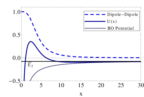
Figure 4: The Born-Oppenheimer potential (dashed) and dipole-dipole potential (dotted) for $\lambda=1$, and total potentials (solid). The horizontal lines are the two-body threshold ${\bar{E}}_{2}\equiv\left(a_{0}/2\mathcal{Q}_{\rm{eff}}^{2}\right)E_{2}$. All potentials are plotted as functions of $x$, and calculated for $x_{0}=4.0$ and mass ratio $m_{B}/m_{A}=0.05$.

In sharp contrast, the ground and first excited states exhibit around $\lambda\approx 1$ the typical behavior of states avoiding to cross each other. These two states are for small positive $\lambda$, respectively located in the inner and outer “minima” as reflected by their radii in Figure 5. As $\lambda$ increases towards $1$, the ground state is affected more than the first excited state and, eventually, overtakes the first excited state.

At the degeneracy strength any linear combination of the two states are valid solutions. After the crossing they exchange structure properties, but very quickly afterwards the highest-lying abruptly disappear into the continuum. There is not sufficient space in the inner minimum to hold a bound state, whereas the lowest-lying state remains relatively unaffected in the outer minimum.

The relation between total potential, energy and wave function is shown in Fig. 6 for the ground state around the point of avoided crossing. The barrier of the potential is almost unchanged with the height $\approx 0.4\left(2\mathcal{Q}_{\rm{eff}}^{2}/a_{0}\right)$ at $x\approx 2.2$. However, this only reflects that very small variation of $\lambda$ results in a major change of the wave function.

For the smallest repulsion, the wave function is localized inside the barrier, but quickly a tail develops and soon also a peak outside the barrier. Eventually this broad peak in the outer minimum carries all the probability. Tuning to the crossing point allows equal probability in the two minima in this entangled state. Very small strength variation moves the probability to the inner or outer minima in two corresponding clearly distinguishable states. This size variation is reflected in the mean-square radii, shown in Fig. 5.

At this point we want to emphasize that the dipole strength can be simply changed by varying the direction of the dipole relative to the two-dimensional plane where they move. This possibility of essentially manual control of the state, placing it on the left or right of the barrier, simulates controlled entangled states, and may thus provide a playground to simulate a qubit.

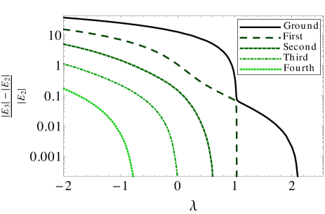
(a)

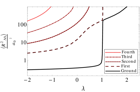
(b)

Figure 5: (a) Three-body energy spectrum, $E_{3}$, with respect to the two-body threshold, $E_{2}$, and (b) mean-square radii of the heavy-heavy distance for the respective states. Both energies and sizes as functions of the strength, $\lambda$, of the dipole potential for a fixed $x_{0}=4.0$ and mass ratio $m_{B}/m_{A}=0.05$.

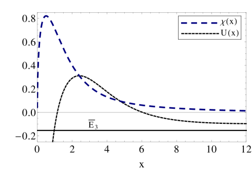
(a) $\lambda=0.95$

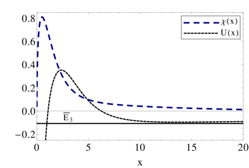
(b) $\lambda=1.0$

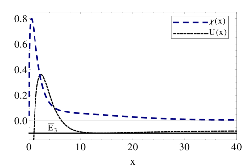
(c) $\lambda=1.012$

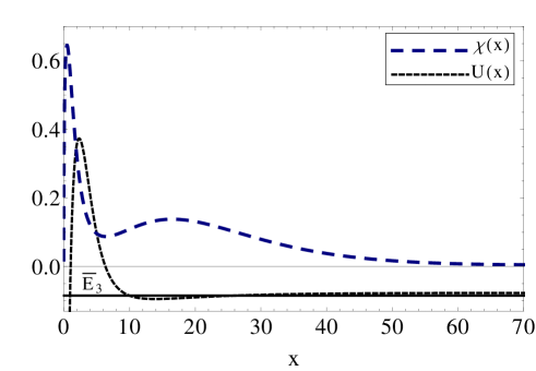
(d) $\lambda=1.025$

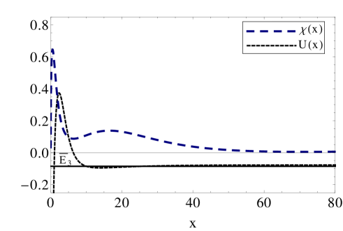
(e) $\lambda=1.035$

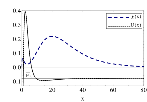
(f) $\lambda=1.050$

Figure 6: Sequence of figures showing how the total potential $U(x)$, three-body energy ${\bar{E}}_{3}\equiv\left(a_{0}/2\mathcal{Q}_{\rm{eff}}^{2}\right)E_{3}$ and the heavy-dipole ground-state wave function $\chi(x)$, change according to the strength of the dipole potential $\lambda$ in the region where there is a more accentuated increase of $\langle R_{AA}^{2}\rangle$. The strength is given just below of each figure, for a fixed $x_{0}=4.0$ and mass ratio $m_{B}/m_{A}=0.05$

These properties depend on the chosen parameters in the calculations. We have fixed the mass ratio, $m_{B}/m_{A}$, and the two-body strength parameterized by $E_{2}$. Decreasing $m_{B}/m_{A}$ or increasing $E_{2}$ must lead to more attractive Born-Oppenheimer potentials: this in turn provides more bound states for a given repulsive dipole strength, $\lambda$, both in the inner but far more in the outer minimum. However, avoided crossings and the produced entangled states for very specific $\lambda$-values would occur each time an inner and an outer localized state become degenerate. Thus, these properties occur rather frequently and not necessarily among the lowest-lying levels.

IV.3 Critical dipole strength

The total potential $U(x)$ as shown in Fig. 4 for one dipole strength has a deep narrow minimum at small distances and a very broad shallow minimum at much larger distances. The details of these characteristic features depend somewhat on the parameter choices, that is mass ratio, $m_{B}/m_{A}$, two-body energy, $E_{2}$, and dipole strength $\lambda$. The number of bound states below the two-body continuum threshold increases dramatically with decreasing $m_{B}/m_{A}$, but most of these states would be localized in the outer minimum.

The barrier created by the dipole repulsion would push the states away, and the less room at small distance would severely limit the corresponding number of bound states. For any given mass ratio, the increase in $\lambda$ pushes all energies towards the continuum threshold. First, all the small-distance states disappear and then much more slowly one by one the large-distance localized states also disappear. For sufficiently large $\lambda$, no three-body bound states are left even though the light particle is bound to each of the heavy ones. This happens for a critical strength value $\lambda=\lambda_{c}$, in the dipole-dipole potential.

It is tempting to estimate $\lambda_{c}$ by use of the Landau criterion, that is by having a negative two-dimensional volume of the potential. We can integrate analytically both the Born-Oppenheimer and the dipole potential. The condition for vanishing volume below the two-body threshold is then to integrate the total potential from Eq. (18), equate to zero and determine $\lambda$; that is

$$\int_{0}^{\infty}dx\ x\left[\frac{a_{0}}{2\mathcal{Q}_{\rm{eff}}^{2}}\bigg{(}\epsilon(x)+|E_{2}|\bigg{)}+\frac{\lambda x_{0}^{3}}{x^{3}+x_{0}^{3}}\right]=0\;.$$ (20)

The first of these integrals is obtained by partial integration using the fact that $\lim_{x\rightarrow\infty}\epsilon(x)=-|E_{2}|$

$$\int_{0}^{\infty}dx\ x\left[\frac{a_{0}}{2\mathcal{Q}_{\rm{eff}}^{2}}|E_{2}|(\bar{\epsilon}(x)+1)\right]$$ (21)

$$= -\frac{a_{0}}{2\mathcal{Q}_{\rm{eff}}^{2}}|E_{2}|\int_{0}^{\infty}\frac{x^{2}}{2}\frac{d\bar{\epsilon}(x)}{dx}dx\;,$$

where $\bar{\epsilon}(x)\equiv\epsilon(x)/|E_{2}|$. Changing variable, $R=\left(a_{0}/2\right)x$ in Eq. (4) to write

$$\ln\left[\bar{\epsilon}(x)\right]=2K_{0}\left(y\right),$$ (22)

where $y\equiv\left(e^{\gamma}\mu_{B,AA}/2\mu_{AA}\right)\sqrt{\bar{\epsilon}(x)}\ x$ we can find an expression for $d\bar{\epsilon}(x)$

$$d\bar{\epsilon}(x)=2\bar{\epsilon}(x)\frac{dK_{0}(y)}{dy}dy.$$ (23)

Finally, after a new partial integration, we write the contribution for the BO potential in the Landau criterion as

$$-4e^{-2\gamma}\frac{a_{0}}{2\mathcal{Q}_{\rm{eff}}^{2}}|E_{2}|\left(\frac{\mu_{AA}}{\mu_{B,AA}}\right)\int_{0}^{\infty}dy\ y^{2}K^{\prime}_{0}(y)=2.$$ (24)

The second integral in Eq. (20) gives

$$\int_{0}^{\infty}dx\ \frac{x}{x^{3}+x_{0}^{3}}=\frac{2\pi}{3\sqrt{3}x_{0}}\;.$$ (25)

Combining the results, we get the critical $\lambda$-value

$$x_{0}^{2}\lambda_{c}=\left(\frac{\mu_{AA}}{\mu_{B,AA}}\right)\frac{3\sqrt{3}}{\pi}\;.$$ (26)

Since $\mu_{AA}/\mu_{B,AA}\approx 0.5m_{A}/m_{B}$ we get that $x_{0}^{2}\lambda_{c}\approx 0.83m_{A}/m_{B}$, which predicts linear relation between $\lambda_{c}$ and the mass ratio. In Table 2 we demonstrate that this prediction is far from being even qualitatively correct. On the other hand we find that the critical dipole strength for constant $x_{0}$ accurately is quadratic in the mass ratio.

Table 2: Critical strengths computed numerically $\lambda_{c}^{(N)}$, as function of mass ratio $m_{B}/m_{A}$ for $x_{0}=4.0$.

$m_{B}/m_{A}$	$\left(\mu_{B,AA}/\mu_{AA}\right)\lambda_{c}^{(N)}$	$\left(\mu_{B,AA}\mu_{AA}\right)^{2}\lambda_{c}^{(N)}$
0.001	17.891	0.0357
0.005	3.580	0.0357
0.010	1.790	0.0357
0.050	0.366	0.0357
0.100	0.191	0.0361

The failure is easily explained since the potentials are far from being weak as required for the Landau criterion to be valid. The positive contribution from the huge barrier has no influence on the outer minimum where bound states can exist completely independent of the small distance behavior. This is related to the rather short range of the dipole potential. Note that a short-distance potential like a Gaussian would make it even worse. The critical strength for such potentials can only be related to the sizes of their tails at distances where the bound states are localized.

Thus, the properties of the outer minimum are decisive. We then investigate the total potential for large $R$. It is convenient to use the dimensionless measure, $s(R)$, defined in BelJPB2013 , that is

$$s(R)=\sqrt{\frac{2\mu_{B,AA}|E_{2}|}{\hbar^{2}}}R\;.$$ (27)

The total potential below $E_{2}$, $U(x)-\left(a_{0}/2\mathcal{Q}_{\rm{eff}}^{2}\right)|E_{2}|$, in dimensionless units, using the approximation for large values of $R$ (or $s(R)$ or $x(R))$ in the Born-Oppenheimer potential BelJPB2013 , is written as

$$U(s)-\frac{a_{0}}{2\mathcal{Q}_{\rm{eff}}^{2}}|E_{2}| = \frac{a_{0}}{2\mathcal{Q}_{\rm{eff}}^{2}}|E_{2}|\left[-1-\sqrt{2\pi}\frac{e^{-s}}{\sqrt{s}}\right]$$

$$+ \lambda x_{0}^{3}\left(\frac{a_{0}}{2s}\sqrt{\frac{2\mu_{B,AA}|E_{2}|}{\hbar^{2}}}\right)^{3},$$

$$U(s) = \frac{e^{2\gamma}}{4}\left(\frac{\mu_{B,AA}}{\mu_{AA}}\right)\left[\left(\frac{\mu_{B,AA}}{\mu_{AA}}\right)^{2}\frac{e^{\gamma}}{2s^{3}}\ \lambda x_{0}^{3}\right.$$ (28)

$$- \left.\sqrt{2\pi}\frac{e^{-s}}{\sqrt{s}}\right]\;,$$

where we assumed that $x\gg x_{0}$ and replaced the asymptotic form of $\epsilon(x)$ for large arguments. Note that we replaced $\mathcal{Q}_{\rm{eff}}$ and $a_{0}$, respectively, by Eqs. (7) and (8). When both Eq. (IV.3) and its derivative with respect to $s$ are zero at the same point in space, the total potential has a minimum value which precisely is above the infinitesimally small attraction sufficient to support a bound state. This potential is non-negative for all large values of $s$. The solutions to these two equations are $s=5/2$ and $\lambda=\lambda_{c}$, where

$$\lambda_{c}=\left(\frac{\mu_{AA}}{\mu_{B,AA}}\right)^{2}\frac{2\sqrt{2\pi}}{x_{0}^{3}e^{\gamma}}s^{5/2}e^{-s}\;.$$ (29)

Inserting $s=5/2$ and the numerical values we then obtain

$$\lambda_{c}=0.035676\ \left(\frac{\mu_{AA}}{\mu_{B,AA}}\right)^{2}\;,$$ (30)

which is precisely obtained by the explicite numerical calculation shown in Table 2.

The precision in this prediction is remarkable. The analytic result is obtained by assuming that even an infinitesimally small attraction at large distance would be able to support a bound state. It seems to be violating the Landau criterion which is a global property for globally weak potentials. We interprete the above result by arguing that the possibly large positive potentials at small distance are irrelevant since that part cannot provide any binding. We can then as well change the total potential to be zero in all space except at the large distances where a small attractive pocket is left for sufficiently large $\lambda$. Certainly this new potential would be globally very weak since it is zero except at large distance where it is exponentially or cubically small. Since the new potential also must have more bound states than the initial potential, we can use the original Landau argument and determine when there is not even an infinitesimally small attraction left.

IV.4 Experimental possibilities

In this subsection we compare our results with real systems to see whether they are experimentally feasible. The heavy subsystem, generically represented by the letter $A$, may be a magnetic or electric dipole. Similarly to the case of neutral atoms, where we can define a characteristic van der Waals length ($\ell_{\rm vdW}$) that divides the fields of chemistry and physics BraPR2006 , we may also define a characteristic dipole length, $R_{0}$ BohNJP2009 . Both lengths, as well as the Bohr radius ($a_{0}^{B}$), are defined equating the typical kinetic energy $\hbar^{2}/(\mu_{AA}L^{2})$ and the potential energies: Coulomb $e^{2}/L$ ($L\equiv a_{0}^{B}$), van der Waals $C_{6}/L^{6}$ ($L\equiv\ell_{\rm vdW}$) and dipole $CD^{2}/L^{3}$ ($L\equiv R_{0}$). Thus, the dipole length is given by $R_{0}=\mu_{AA}CD^{2}/\hbar^{2}$.

The dipole length $R_{0}$ is very different for each system in such a way we cannot define an overall dipole length scale. However, using the dipole length for each system, we may study what the atom-dipole scattering length would be to unbind the three-body system using the critical $\lambda$ derived in the previous section.

From Eqs. (19) and (29) and writing explicitly the effective charge and radius given, respectively, by Eqs. (7) and (8), we may write the ratio

$$\left(\frac{\lambda}{\lambda_{c}}\right) = \frac{2}{\sqrt{\pi}s^{5/2}e^{-s}}\left(\frac{|E_{2}|\mu_{B,AA}x_{0}^{2}}{\hbar^{2}}\right)^{3/2}\frac{CD^{2}}{|E_{2}|}$$ (31)

$$= \frac{64e^{-3\gamma}}{\sqrt{2\pi}s^{5/2}e^{-s}}\left(\frac{|E_{2}|\mu_{AA}R_{0}}{\hbar^{2}}\right)^{3}\frac{CD^{2}}{|E_{2}|},$$ (32)

where $x_{0}=2R_{0}/a_{0}$ and the two-body binding energy $|E_{2}|$ in two dimensions for the shallow dimer in the unitary limit is given by BraPR2006

$$|E_{2}|=4e^{-2\gamma}\frac{\hbar^{2}}{\mu_{AB}a^{2}},$$ (33)

where $a$ is the two-body scattering length in 2D. For a magnetic dipole the constants are given by $C=1/c^{2}$ and $D^{2}=\mu^{2}$, where the dipole moment $\mu$ should be in units of the Bohr magneton, $\mu_{B}{\equiv}(e\hbar)/(2m_{e})$. Then, the ratio is given by

$$\left(\frac{\lambda}{\lambda_{c}}\right)_{{\rm MAG}}=\frac{256e^{(s-7\gamma)}\mu^{2}\mu_{AA}^{3}R_{0}^{3}}{137^{2}\sqrt{2\pi}s^{5/2}\mu_{B}^{2}\mu_{AB}^{2}m_{e}a_{0}^{B3}}\left(\frac{a_{0}^{B}}{a}\right)^{4},$$

where $s=5/2$.

For an electric dipole, we have $C=1$ and $D^{2}=d^{2}$, where the dipole moment $d$ should be in atomic units $d_{0}\equiv ea_{0}^{B}$. Then, the ratio for an electric dipole reads:

$$\left(\frac{\lambda}{\lambda_{c}}\right)_{{\rm EL}}=\frac{1024e^{(s-7\gamma)}d^{2}\mu_{AA}^{3}R_{0}^{3}}{\sqrt{2\pi}s^{5/2}d_{0}^{2}\mu_{AB}^{2}m_{e}a_{0}^{B3}}\left(\frac{a_{0}^{B}}{a}\right)^{4}.$$

These $\lambda$-ratios increase with dipole moment, length and mass, while decreasing with light mass and heavy-light scattering length. Thus, for a given three-body system we can determine which scattering length, $a$, must be exceeded to allow any bound state structure. The tunneling effect occurs for a range of smaller $\lambda$’s. It is worth mentioning that the tunneling effect, and consequently the avoid crossings, does not happen for all values of $x_{0}$ used to regularize the dipole potential at short distances. In order to have the tunneling, $x_{0}$ should roughly be smaller than 7 as for larger values the minimum located at large distances disappears and there is no bound state on the right side of the barrier. $x_{0}$ is given by

$$x_{0}=4\sqrt{2}e^{-2\gamma}\left(\frac{R_{0}}{a}\right)\frac{\mu_{AA}}{\sqrt{\mu_{B,AA}\mu_{AB}}}.$$ (34)

Let us consider some systems where the light particle is ⁶Li and the two identical heavy particles are either molecules with electric dipoles or atoms with magnetic dipoles. These systems are listed in Table 3 with respective dipole moments, lengths and masses along with the limiting two-body scattering lengths to bind the three-body systems ($\lambda=\lambda_{c}$) and the $x_{0}$-values corresponding to the short-range parameter that regularizes the dipole potential.

We conclude that although some of these scattering lengths are rather large they are all within present-day experimental possibilities and, furthermore, the $x_{0}$-values are all inside the range for tunneling to be observed.

Table 3: Experimental properties of each dipole $A$ represented in the first column. The second column shows the values of the electric or magnetic dipole moments. Electric dipole moments are given in Debye (D) units, 1 Debye$=0.3934ea_{0}^{B}$ ($e$ is the electron charge, $a_{0}^{B}=\hbar^{2}/(m_{e}e^{2})=0.53$ Å  is the Bohr radius and $m_{e}$ the mass of the electron), and magnetic dipole moments are given in units of $\mu_{B}$. In the third column we give the dipole length in units of $a_{0}^{B}$. The last two columns give the scattering length that gives $\lambda=\lambda_{c}$ and the value of $x_{0}$ used to regulate the dipole potential at short distances.

Dipole(A)	Moments	$R_{0}/a_{0}^{B}$	$a/a_{0}^{B}$	$x_{0}$
Singlet 40K-87Rb NiScience2008	0.57 D	$4\times 10^{3}$	25275.5	3.12
87Rb-133Cs DanThesis	1.25 D	$3\times 10^{4}$	253717	3.97
87Rb DanThesis	0.5 $\mu_{B}$	0.2	1.0	2.7
133Cs DanThesis	0.75 $\mu_{B}$	0.6	3.9	3.16
164Dy TanPRA2015	10 $\mu_{B}$	195	1275	3.86
52Cr GriPRL2006	6 $\mu_{B}$	15	63.23	2.05
167Er2 FriPRL2015	14 $\mu_{B}$	1600	12357.1	6.5

V Summary and Conclusions

We studied a three-body system composed of one light and two heavy dipoles, all confined to two spatial dimensions. We used a zero-range interaction between the light and each of the two identical heavy dipoles. This extremely short-range interaction has several advantages: first, it serves as a schematic prototype of a short-range interaction; second, the properties can be semi-analytically derived; and third, the results are universal by definition. The strength is parametrized in terms of the light-heavy system binding energy which then is one of our input parameters. We limit ourselves to a small light-heavy mass ratio allowing the use of the Born-Oppenheimer approximation for an effective potential between the two heavy particles.

The two slowly moving heavy dipoles may also interact directly in addition to the Born-Oppenheimer potential. Here we only considered the realistic possibility of the dipole-dipole interaction which has an inverse cubic dependence on their separation. The strength of this interaction is, besides the size of the dipole moment, determined by the direction of the dipole moments relative to the two-dimensional planar confinement. Adjusting this orientation, which can be achieved experimentally through external fields, the interaction can vary from an attractive to a repulsive potential passing through zero. We have in this work essentially considered only the repulsive and vanishing potentials.

After having established the formalism, we discussed the three-body properties emerging from the Born-Oppenheimer potential and vanishing direct heavy-heavy interaction. The light particle generates an effective interaction as a consequence of its exchange between the two heavy particles. Therefore, the lighter the atom the easier it can be exchanged which then increases the heavy-heavy effective attraction. The number of excited states then increases with decreasing mass ratio, and it is in this way controlled by the constituents of the trap.

Through the Born-Oppenheimer procedure we derived an analytic expression for the wave function depending on the three-body Jacobi relative coordinates. We rewrite and exhibit the wave function in terms of two dimensionless coordinates and a dimensionless scale parameter. The logarithmic divergence is clearly seen when one of the heavy particles is on top of the light one. This coordinate-space wave function may be used in other “realistic” calculations as input to parameterize the large-distance universal tail of the wave function.

The effective potential is Coulomb-like at small distances with an effective charge proportional to the square root of the two-body energy divided by the light particle mass. The corresponding Coulomb degeneracy arising from the angular momentum and radial node quantum numbers is very accurate for the lowest-lying well bound states. The systematic deviation from the Coulomb results is traced to the next order attractive correction terms which are a sum of a constant and a slowly varying logarithmic term. The Coulomb-like behavior is slowly destroyed as the energies approach the two-body continuum threshold.

We included the dipole-dipole interaction, oriented to produce repulsion, and minimally regularized for zero separation. The total heavy-heavy potential is now the result of a competition between the two contributions. At the smallest distances, the Coulomb-like attraction survives with a translated energy scale. For moderate repulsive strengths, a barrier appears before a broad minimum at larger distances. Increasing the repulsion affects the short-distance localized states much more than states in the broad minimum. Specific strengths therefore lead to crossing of the inner and outer localized states. At the avoided crossing points two levels are nearly degenerate and each is a mixture of the two structures. Characteristic signals of this type of tunneling phenomenon are the avoided crossing spectrum, and an exchange of properties such as mean square radii between the two levels involved.

Increasing the heavy-heavy repulsion sufficiently the bound states disappear one by one until no bound state is left and the three-body system is unstable towards emission of one of the heavy particles. This defines a critical dipole strength as a function of mass ratio and two-body strength. We derived the Landau criterion analytically for this critical strength, but concluded that it is wrong both quantitatively as well as qualitatively. The relatively short-range nature of the dipole repulsion requires a large strength to exclude all bound states. The resulting large positive barrier at intermediate distances violates the assumption of a weak potential for validity of the Landau criterion. The last bound state owes its existence to a tiny attraction at the outer edge of the exponentially decaying Born-Oppenheimer potential. When this pocket is wiped out, the repulsive dipole has just passed the critical strength, which we analytically and numerically calculate to be proportional to the square of the inverse mass ratio.

The full Faddeev calculation SaPRA2016 is numerically feasible in 2D. However, the Born-Oppenheimer approximation separates fast and slow motion and provides semi-analytic results which in simple terms explain the underlying complicated physics. This is especially highlighted in the Coulomb-like short-distance part of the effective potential which explicitly shows the physical reason for the increase of bound states when the mass ratio is decreased. This also shows the crucial difference from the $1/r^{2}$ potential in 3D which is responsible for the appearance of the scaling laws characteristic of Efimov states.

The Born-Oppenheimer established attractive $1/r$ effective short-range potential reveals the difference between studies using the present dipolar potential and zero-range interactions BelJPB2013 ; SaPRA2016 . Tuning the strengths of the finite-range (dipolar) and the short-range Born-Oppenheimer potentials can emphasize short or long-range behavior, or allowing equal influence. This opens a field of new physics which depends on both the strength and shape of the finite-range interaction. This variation generates interesting phenomena in energy spectra and mean-square radii that is not possible when assuming only attractive short-range interactions. Consequently, the results are no longer universal.

The study made in this paper can be tested experimentally and easily extended to three distinguishable particles. The possibility to localize degenerate wave functions in the two minima by tuning the interactions may provide an interesting alternative to controlled transfer of quantum information between these entangled states. The possibility to vary the strength by changing angles of the dipoles combined with the Feshbach resonance technique to control the short-range interaction produces a very rich playground to study few-body correlations.

- (1) C. J. Pethick and H. Smith Bose-Einstein Condensation in Dilute Gases (Cambridge University Press, New York, 2008).
- (2) I. Bloch, J. Dalibard and W. Zwerger, Rev. Mod. Phys. 80, 885 (2008).
- (3) C. Chin, R. Grimm, P. Julienne and E. Tiesinga, Rev. Mod. Phys. 82, 1225 (2010).
- (4) E. Nielsen, D. V. Fedorov, A. S. Jensen and E. Garrido, Phys. Rep. 347, 373 (2001).
- (5) E. Braaten and H. W. Hammer, Phys. Rep. 428, 259 (2006).
- (6) D. Blume, Rep. Prog. Phys. 75, 046401 (2012).
- (7) T. Frederico, L. Tomio, A. Delfino, M. R. Hadizadeh and M. T. Yamashita, Few-Body Syst. 51, 87 (2011).
- (8) A. C. Phillips, Nucl. Phys. A 107, 209 (1968).
- (9) F. Coester, S. Cohen, B. Day and C. M. Vincent, Phys. Rev. C 1, 769 (1970).
- (10) J. A. Tjon, Phys. Lett. 56B, 217 (1975).
- (11) V. Efimov, Phys. Lett. B 33, 563 (1970); V. Efimov, Nucl. Phys. A 362 45 (1981).
- (12) L. H. Thomas, Phys. Rev. 47, 903 (1935).
- (13) D. E. Pritchard, Phys. Rev. Lett. 51, 1336 (1983).
- (14) A. L. Migdall et al., Phys. Rev. lett. 54, 2596 (1985).
- (15) J. Schmiedmayer, Appl. Phys. B 60, 169 (1995).
- (16) F. Werner, Y. Castin, Phys. Rev. A 86, 053633 (2012).
- (17) F. F. Bellotti and M. T. Yamashita, Few-Body Syst. 56, 905 (2015).
- (18) M. T. Yamashita, F. F. Bellotti, T. Frederico, D. V. Fedorov, A. S. Jensen and N. T. Zinner, J. Phys. B 48, 025302 (2015).
- (19) L. W. Bruch and J. A. Tjon, Phys. Rev. A 19, 425 (1979).
- (20) T. K. Lim and P. A. Maurone, Phys. Rev. B 22, 1467 (1980).
- (21) S. K. Adhikari, A. Delfino, T. Frederico, I. D. Goldman and L. Tomio, Phys. Rev. A 37, 3666 (1988).
- (22) T. K. Lim and B. Shimer, Z. Phys. A 297, 185 (1980).
- (23) J. I. Cirac and P. Zoller, Phys. Rev. Lett. 74, 4091 (1995).
- (24) K. Eckert et al., Phys. Rev. A 66, 042317 (2002).
- (25) F. W. Strauch et al., Phys. Rev. A 77, 050304(R) (2008).
- (26) K. B. Soderberg, N. Gemelke and C. Chin, New. J. Phys. 11, 055022 (2009).
- (27) T. D. Ladd et al., Nature 464, 45 (2010).
- (28) W. S. Bakr, J. I. Gillen, A. Peng, S. Fölling and M. Greiner, Nature 462, 74 (2008)
- (29) C. Weitenberg at al., Nature 471, 319 (2011).
- (30) M. A. Baranov, Phys. Rep. 464, 71 (2008).
- (31) T. Lahaye, C. Menotti, I. Santos, M. Lewenstein and T. Pfau, Rep. Prog. Phys. 126401 (2009).
- (32) M. Kiffner, W. Li and D. Jaksch, Phys. Rev. Lett. 111 233003 (2013); M. Kiffner, M. X. Huo, W. Li and D. Jaksch, Phys. Rev. A 89, 052717 (2014).
- (33) K. K. Hansen, D. V. Fedorov, A. S. Jensen and N. T. Zinner, Phys. Scr. 90 125002 (2015).
- (34) K. K. Ni et al., Science 322, 231 (2008).
- (35) T. Takekoshi, Phys. Rev. Lett. 113, 205301 (2014).
- (36) P. K. Molony et al., Phys. Rev. Lett. 113, 255301 (2014).
- (37) J. W. Park, S. A. Will and M. W. Zwierlein, Phys. Rev. Lett. 114, 205302 (2015).
- (38) M. Guo et al., Phys. Rev. Lett. 116, 205303 (2016).
- (39) F. F. Bellotti, T. Frederico, M. T. Yamashita, D. V. Fedorov, A. S. Jensen and N. T. Zinner, J. Phys. B 46, 055301 (2013).
- (40) J. H. Sandoval, F. F. Bellotti, A. S. Jensen and M. T. Yamashita, Phys. Rev. A 94, 022514 (2016).
- (41) S. S. Avancini, J. R. Marinelli and G. Krein, J. Phys. A 36, 9045 (2003).
- (42) J. L. Bohn, M. Cavagnero and C. Ticknor, New J. Phys. 11, 055039 (2009).
- (43) D. J. McCarron, Ph.D. Thesis, Durham University, 2011.
- (44) Y. Tang et al., Phys. Rev A 92, 022703 (2015).
- (45) A. Griesmaier et al., Phys. Rev Lett 97, 250402 (2006).
- (46) A. Frisch et al., Phys. Rev Lett 115, 203201 (2015).