Some Computational and Theoretical Aspects of the Exponentiated Generalized Nadarajah-Haghighi Distribution

VedoVatto    T.1,2,∗ Corresponding author. Email: thiagovedovatto@gmail.com    Nascimento    A. D. C.2    Miranda Filho    W. R.2    Lima    M. C. S.2    Pinho    L. G. B.3 and Cordeiro    G. M.2
1Instituto Federal de Educação, Ciência e Tecnologia de Goiás, Goiânia, Brazil
2Departamento de Estatística, Universidade Federal de Pernambuco, Recife, Brazil 3Departamento de Estatística e Matemática Aplicada, Universidade Federal do Ceará, Fortaleza, Brazil
(Received: 00 Month 200x \sepAccepted in final form: 00 Month 200x)
Abstract

Real data from applications in the survival context have required the use of more flexible models. A new four-parameter model called the Exponentiated Generalized Nadarajah-Haghighi (EGNH) distribution has been introduced in order to verify this requirement. We prove that its hazard rate function can be constant, decreasing, increasing, upside-down bathtub and bathtub-shape. Theoretical essays are provided about the EGNH shapes. It includes as special models the exponential, exponentiated exponential, Nadarajah-Haghighi’s exponential and exponentiated Nadarajah-Haghighi distributions. We present a physical interpretation for the EGNH distribution and obtain some of its mathematical properties including shapes, moments, quantile, generating functions, mean deviations and Rényi entropy. We estimate its parameters by maximum likelihood, on which one of the estimates may be written in closed-form expression. This last result is assessed by means of a Monte Carlo simulation study. The usefulness of the introduced model is illustrated by means of two real data sets. We hope that the new distribution could be an alternative to other distributions available for modeling positive real data in many areas.
{classcode} Primary 62E10 \sepSecondary 62P30.

keywords:
Exponentiated Exponential \sepExponentiated generalized family \sepNadarajah-Haghighi’s exponential \sepT-X family

1 Introduction

In recent years, several ways of generating new continuous distributions have been proposed in survival analysis to provide flexibility and new forms for the hazard rate function (hrf). A detailed study about ‘the evolution of the methods for generalizing classic distributions’ was made by Lee et al. (2013). Most of them are special cases of the T-X class defined by Alzaatreh et al. (2013). This class of distributions extends some recent families such as the beta-G pioneered by Eugene et al. (2002), the gamma-G defined by Zografos and Balakrishnan (2009), the Kw-G family proposed by Cordeiro and Castro (2011) and the Weibull-G introduced by Bourguignon et al. (2014).

The process to construct a generator based on the T-X class is given as follows. Let r(t)𝑟𝑡r(t) be the probability density function (pdf) of a random variable T[a,b]𝑇𝑎𝑏T\in[a,b] for <a<b<𝑎𝑏-\infty<a<b<\infty and let W[G(x)]𝑊delimited-[]𝐺𝑥W[G(x)] be a mapping under the following conditions:

  • W[G(x)][a,b]𝑊delimited-[]𝐺𝑥𝑎𝑏W[G(x)]\in[a,b];

  • W[G(x)]𝑊delimited-[]𝐺𝑥W[G(x)] is monotonically non-decreasing and differentiable;

  • W[G(x)]a𝑊delimited-[]𝐺𝑥𝑎W[G(x)]\rightarrow a as x𝑥x\rightarrow-\infty and W[G(x)]b𝑊delimited-[]𝐺𝑥𝑏W[G(x)]\rightarrow b as x𝑥x\rightarrow\infty.

The new T-X generator has cumulative distribution function (cdf) and pdf given, respectively, by

F(x)=aW[G(x)]r(t)𝑑tandf(x)={ddxW[G(x)]}r{W[G(x)]}.formulae-sequence𝐹𝑥superscriptsubscript𝑎𝑊delimited-[]𝐺𝑥𝑟𝑡differential-d𝑡and𝑓𝑥𝑑𝑑𝑥𝑊delimited-[]𝐺𝑥𝑟𝑊delimited-[]𝐺𝑥F(x)=\int_{a}^{W[G(x)]}r(t)dt\quad\text{and}\quad f(x)=\left\{\frac{d}{dx}W[G(x)]\right\}r\left\{W[G(x)]\right\}.

The choice of W()𝑊W(\cdot) is intrinsically associated with the cdf of T𝑇T. For example, if T𝑇T follows a beta distribution, W()𝑊W(\cdot) can be the identity function, leading to the beta-G family. On the other hand, if T𝑇T follows a gamma distribution, W[G(x)]𝑊delimited-[]𝐺𝑥W[G(x)] must be a function such that W:[0,1][0,):𝑊010W{:}[0,1]\rightarrow[0,\infty). Examples of functions that satisfy this restriction are: W[G(x)]=log[1G(x)]𝑊delimited-[]𝐺𝑥1𝐺𝑥W[G(x)]=-\log[1-G(x)], W[G(x)]=log[G(x)]𝑊delimited-[]𝐺𝑥𝐺𝑥W[G(x)]=-\log[G(x)] and W[G(x)]=G(x)/[1G(x)]𝑊delimited-[]𝐺𝑥𝐺𝑥delimited-[]1𝐺𝑥W[G(x)]=G(x)/[1-G(x)].

Cordeiro et al. (2013) proposed an interesting family in the T-X class inspired by the second type Kumaraswamy distribution. We refer to this family as the exponentiated generalized (EG) family, which has cdf and pdf (for x>0𝑥0x>0) given, respectively, by

F(x)={1[1G(x)]α}β𝐹𝑥superscript1superscriptdelimited-[]1𝐺𝑥𝛼𝛽F(x)=\{1-[1-G(x)]^{\alpha}\}^{\beta} (1)

and

f(x)=αβg(x)[1G(x)]α1{1[1G(x)]α}1β,𝑓𝑥𝛼𝛽𝑔𝑥superscriptdelimited-[]1𝐺𝑥𝛼1superscript1superscriptdelimited-[]1𝐺𝑥𝛼1𝛽f(x)=\frac{\alpha\beta g(x)[1-G(x)]^{\alpha-1}}{\{1-[1-G(x)]^{\alpha}\}^{1-\beta}}, (2)

where α>0𝛼0\alpha>0 and β>0𝛽0\beta>0 are two additional shape parameters that can control both tail weights. One can note that equations (1) and (2) do not involve any complicated function, which is an advantage when compared to the beta and gamma families. Further, the EG family is nothing more than a sequential application of the Lehmann type 2 alternative to the exponentiated class. Setting α=1𝛼1\alpha=1 gives the exponentiated-G (Lehmann type 1) class defined by Gupta et al. (1998).

The best benefit of the EG family is its ability to fitting skewed data. This class is also dual of the Kw-G family and has similar properties of the beta-G family and some advantages in terms of tractability. Some special models in this class have been studied recently. The EG-inverse Gaussian by Lemonte and Cordeiro (2011), the EG-generalized gamma by Silva et al. (2015), the EG-inverse Weibull by Elbatal and Muhammed (2014) and the EG-Gumbel by Andrade et al. (2015) distributions are special cases obtained by taking G(x)𝐺𝑥G(x) to be the cdf of the inverse Gaussian, generalized gamma, inverse Weibull and Gumbel distributions, respectively. Hence, each new EG distribution can be generated from a specified G𝐺G distribution.

A new generalization of the exponential law as an alternative to the gamma and Weibull models has been proposed by Nadarajah and Haghighi (2011), which model has cdf given by (for x>0𝑥0x>0)

G(x)=1e1(1+ax)b,𝐺𝑥1superscripte1superscript1𝑎𝑥𝑏G(x)=1-\operatorname{\mathrm{e}}^{1-(1+ax)^{b}}, (3)

where a>0𝑎0a>0 and b>0𝑏0b>0. Its pdf reduces to

g(x)=ab(1+ax)b1e1(1+ax)b.𝑔𝑥𝑎𝑏superscript1𝑎𝑥𝑏1superscripte1superscript1𝑎𝑥𝑏g(x)=ab(1+ax)^{b-1}\operatorname{\mathrm{e}}^{1-(1+ax)^{b}}. (4)

This model is called the Nadarajah-Haghighi’s exponential (denoted by ZNH(a,b)similar-to𝑍NH𝑎𝑏Z\sim\operatorname{\mathrm{NH}}(a,b)) because the exponential is a special case when b=1𝑏1b=1. This bi-parametric model has been used for modeling lifetime data. The pdf (4) is always monotonically decreasing with g(0)=ab𝑔0𝑎𝑏g(0)=ab. Nadarajah and Haghighi (2011) pointed out that this distribution has an attractive feature of always having the zero mode. They also showed that larger values of b𝑏b lead to faster decay of the upper tail. Additionally, the hrf can be monotonically increasing for b>1𝑏1b>1, and monotonically decreasing for b<1𝑏1b<1. For b=1𝑏1b=1, the hrf becomes constant. So, the major weakness of the NH distribution is its inability to accommodate non-monotone hrfs (i.e. bathtub-shaped and upside-down bathtub).

Several extensions of the NH model have been proposed in recent years such as the following distributions: the generalized power Weibull (GPW), Kumaraswamy generalized power Weibull (KGPW), exponentiated (Lehmann type 1) Nadarajah-Haghighi (ENH), gamma (Zografos-Balakrishnan type) Nadarajah-Haghighi (GNH), Poisson gamma (also of Zografos-Balakrishnan type) Nadarajah-Haghighi (PGNH), transmuted (quadratic random transmuted map) Nadarajah-Haghighi (TNH), Kumaraswamy Nadarajah-Haghighi (KNH), exponentiated (Lehmann type 2) Nadarajah-Haghighi (E2NH) (submodel of the KNH), modified Nadarajah-Haghighi (MNH), Marshall-Olkin Nadarajah-Haghighi (MONH) and beta Nadarajah-Haghighi (BNH). These distributions and their corresponding authors are listed in Table 1.

Table 1: Nadarajah-Haghighi extensions
Distribution Author(s)
GPW Nikulin and Haghighi (2006, 2009)
ENH Lemonte (2013) and Abdul Moniem (2015)
GNH Ortega et al. (2015) and Bourguignon et al. (2015)
PGNH Ortega et al. (2015)
TNH Ahmed et al. (2015)
KNH Lima (2015)
MNH El Damcese and Ramadan (2015)
MONH Lemonte et al. (2016)
KGPW Selim and Badr (2016)
BNH Dias (2016)

In this paper, we obtain a natural extension of the NH distribution, which we refer to as the exponentiated generalized Nadarajah-Haghighi (EGNH) distribution. The first motivation for introducing the new distribution is based on the fact that it has simple expressions for the pdf and hrf and, as a consequence, a simpler statistical inference process. Second, the flexibility of the new distribution to describe complex positive real data is concluded since this hrf can present constant, decreasing, increasing, unimodal, bathtub-shaped and upside-down bathtub forms. Due to the great flexibility of its hrf, it can provide a good alternative to many existing lifetime distributions to model real data. Therefore, the beauty and importance of the new distribution lies in its ability to model monotone as well as nonmonotone hrfs, which are quite common in reliability and biological studies.

So, our main aim is to propose a new four-parameter distribution, which extends the exponential, NH and ENH distributions, with the hope that it may provide a ‘better fit’ compared to other lifetime distributions in certain practical situations. Additionally, we provide a comprehensive account of the mathematical properties of the introduced distribution. The formulae related with the new distribution are simple and manageable, and, with the use of modern computer resources and their numerical capabilities, the proposed distribution may prove to be an useful addition to the arsenal of applied statisticians in areas like biology, medicine, economics, reliability, engineering, among others.

The paper is outlined as follows. In Section 2, we introduce the new distribution, some of its basic properties and provide plots of the pdf and hrf. Section 3 deals with nonstandard measures of skewness and kurtosis. Linear representations for the pdf and cdf are presented in Section 4 and explicit expressions for the moments are provided in Section 5. Section 6 is devoted to the moment generating function (mgf). The mean deviations are obtained in Section 7. The Rényi entropy is derived in Section 8. In Section 9, we present the order statistics. A procedure to calculate the maximum likelihood estimators (MLEs) of the model parameters is investigated in Section 10. A simulation study illustrating the convergence and consistency of the MLEs is addressed in Section 11. Two applications to real data are provided in Section 12. Finally, Section 13 offers some concluding remarks.

2 The proposed model

The EGNH cdf is obtained by applying (3) in Equation (1)

F(x)={1[e1(1+ax)b]α}β,x>0,formulae-sequence𝐹𝑥superscript1superscriptdelimited-[]superscripte1superscript1𝑎𝑥𝑏𝛼𝛽𝑥0F(x)=\left\{1-\left[\operatorname{\mathrm{e}}^{1-(1+ax)^{b}}\right]^{\alpha}\right\}^{\beta},\quad x>0, (5)

where α,β,a,b>0𝛼𝛽𝑎𝑏0\alpha,\beta,a,b>0 and b1𝑏1b\neq 1. The EGNH pdf can be obtained by applying (3) and (4) in (2) or by differentiating (5):

f(x)=aαbβ(1+ax)b1[e1(1+ax)b]α{1[e1(1+ax)b]α}1β.𝑓𝑥𝑎𝛼𝑏𝛽superscript1𝑎𝑥𝑏1superscriptdelimited-[]superscripte1superscript1𝑎𝑥𝑏𝛼superscript1superscriptdelimited-[]superscripte1superscript1𝑎𝑥𝑏𝛼1𝛽f(x)=\frac{a\alpha b\beta(1+ax)^{b-1}\left[\operatorname{\mathrm{e}}^{1-(1+ax)^{b}}\right]^{\alpha}}{\left\{1-\left[\operatorname{\mathrm{e}}^{1-(1+ax)^{b}}\right]^{\alpha}\right\}^{1-\beta}}. (6)

Henceforth, we denote by XEGNH(α,β,a,b)similar-to𝑋EGNH𝛼𝛽𝑎𝑏X\sim\operatorname{\mathrm{EGNH}}(\alpha,\beta,a,b) a random variable having pdf (6). So, the EGNH distribution is obtained by adding two shape parameters α𝛼\alpha and β𝛽\beta to the NH distribution. It is necessary to consider b1𝑏1b\neq 1, an additional restriction to the parametric space, to give identifiability to the generated model.

The EGNH distribution has also an attractive physical interpretation whenever α𝛼\alpha and β𝛽\beta are positive integers. Consider a device based on β𝛽\beta independent components in a parallel system. Further, each component is defined in terms of α𝛼\alpha independent subcomponents identically distributed following the NH model in a series system. Assume that the device fails if all β𝛽\beta components fail and each component fails if any subcomponent fails. Let Xj1,,Xjαsubscript𝑋𝑗1subscript𝑋𝑗𝛼X_{j1},\ldots,X_{j\alpha} denote the lifetimes of the subcomponents within the j𝑗jth component, j=1,,β𝑗1𝛽j=1,\ldots,\beta, with common cdf given by (3). Let Xjsubscript𝑋𝑗X_{j} denote the lifetime of the j𝑗jth component and let X𝑋X denote the lifetime of the device. Thus, the cdf of X𝑋X is given by

P(Xx)=𝑃𝑋𝑥absent\displaystyle P(X\leq x)= P(X1x,,Xβx)=P(X1x)β=[1P(X1>x)]β𝑃formulae-sequencesubscript𝑋1𝑥subscript𝑋𝛽𝑥𝑃superscriptsubscript𝑋1𝑥𝛽superscriptdelimited-[]1𝑃subscript𝑋1𝑥𝛽\displaystyle P(X_{1}\leq x,\ldots,X_{\beta}\leq x)=P(X_{1}\leq x)^{\beta}=\left[1-P(X_{1}>x)\right]^{\beta}
=\displaystyle= [1P(X11>x,,X1α>x)]β=[1P(X11>x)α]βsuperscriptdelimited-[]1𝑃formulae-sequencesubscript𝑋11𝑥subscript𝑋1𝛼𝑥𝛽superscriptdelimited-[]1𝑃superscriptsubscript𝑋11𝑥𝛼𝛽\displaystyle\left[1-P(X_{11}>x,\ldots,X_{1\alpha}>x)\right]^{\beta}=\left[1-P(X_{11}>x)^{\alpha}\right]^{\beta}
=\displaystyle= {1[1P(X11x)]α}β.superscript1superscriptdelimited-[]1𝑃subscript𝑋11𝑥𝛼𝛽\displaystyle\left\{1-\left[1-P(X_{11}\leq x)\right]^{\alpha}\right\}^{\beta}.

So, the lifetime of the device obeys the EGNH distribution.

The quantile function (qf) of X𝑋X is determined by inverting (5) (for 0<p<10𝑝10<p<1) as

Q(p)=1a{{1log[(1p1β)1α]}1b1}.𝑄𝑝1𝑎superscript1superscript1superscript𝑝1𝛽1𝛼1𝑏1Q(p)=\frac{1}{a}\left\{\left\{1-\log\left[\left(1-p^{\frac{1}{\beta}}\right)^{\frac{1}{\alpha}}\right]\right\}^{\frac{1}{b}}-1\right\}. (7)

Clearly, the median of the new distribution follows by setting p=1/2𝑝12p=1/2 in (7). We can also use (7) for simulating EGNH random variables by the inverse transform sampling method, which works as follows:

  1. 1.

    Let u𝑢u be an outcome of uniform distribution in the interval [0,1]01[0,1].

  2. 2.

    x=Q(u)𝑥𝑄𝑢x=Q(u) is them an outcome of the EGNH distribution.

Finally, the survival function (sf) and hrf of X𝑋X are given, respectively, by

S(x)𝑆𝑥\displaystyle S(x) =1{1[e1(1+ax)b]α}βandabsent1superscript1superscriptdelimited-[]superscripte1superscript1𝑎𝑥𝑏𝛼𝛽and\displaystyle=1-\left\{1-\left[\operatorname{\mathrm{e}}^{1-(1+ax)^{b}}\right]^{\alpha}\right\}^{\beta}\,\,\,\text{and}
h(x)𝑥\displaystyle h(x) =aαbβ(1+ax)b1[e1(1+ax)b]α1{1[e1(1+ax)b]α}β{1[e1(1+ax)b]α}1β.absent𝑎𝛼𝑏𝛽superscript1𝑎𝑥𝑏1superscriptdelimited-[]superscripte1superscript1𝑎𝑥𝑏𝛼1superscript1superscriptdelimited-[]superscripte1superscript1𝑎𝑥𝑏𝛼𝛽superscript1superscriptdelimited-[]superscripte1superscript1𝑎𝑥𝑏𝛼1𝛽\displaystyle=\frac{a\alpha b\beta(1+ax)^{b-1}\left[\operatorname{\mathrm{e}}^{1-(1+ax)^{b}}\right]^{\alpha}}{1-\left\{1-\left[\operatorname{\mathrm{e}}^{1-(1+ax)^{b}}\right]^{\alpha}\right\}^{\beta}\left\{1-\left[\operatorname{\mathrm{e}}^{1-(1+ax)^{b}}\right]^{\alpha}\right\}^{1-\beta}}. (8)

The reverse hrf of X𝑋X is given by

r(x)=aαbβ(1+ax)b1[e1(1+ax)b]α{1[e1(1+ax)b]α}β=β[FE2NH(x)]βfE2NH(x)𝑟𝑥𝑎𝛼𝑏𝛽superscript1𝑎𝑥𝑏1superscriptdelimited-[]superscripte1superscript1𝑎𝑥𝑏𝛼superscript1superscriptdelimited-[]superscripte1superscript1𝑎𝑥𝑏𝛼𝛽𝛽superscriptdelimited-[]subscript𝐹𝐸2𝑁𝐻𝑥𝛽subscript𝑓𝐸2𝑁𝐻𝑥r(x)=\frac{a\alpha b\beta(1+ax)^{b-1}\left[\operatorname{\mathrm{e}}^{1-(1+ax)^{b}}\right]^{\alpha}}{\left\{1-\left[\operatorname{\mathrm{e}}^{1-(1+ax)^{b}}\right]^{\alpha}\right\}^{\beta}}=\frac{\beta}{\left[F_{E2NH}(x)\right]^{\beta}}\,f_{E2NH}(x)

where FE2NH(x)subscript𝐹𝐸2𝑁𝐻𝑥F_{E2NH}(x) and fE2NH(x)subscript𝑓𝐸2𝑁𝐻𝑥f_{E2NH}(x) are, respectively, the cdf and pdf of E2NH (Lehmann type 2) distribution, which is a special case of the model proposed by Lima (2015) and Selim and Badr (2016). In the following, we address limit distributions, shape and special cases of the EGNH model.

2.1 Limiting behavior of the density

The pdf (6) can take various forms depending on the values of the α𝛼\alpha and β𝛽\beta shape parameters. It is easy to verify that

limx0f(x)={,β<1abα,β=10,β>1andlimxf(x)=0.formulae-sequencesubscript𝑥0𝑓𝑥cases𝛽1𝑎𝑏𝛼𝛽10𝛽1andsubscript𝑥𝑓𝑥0\displaystyle\lim_{x\to 0}f(x)=\begin{cases}\infty,&\beta<1\\ ab\alpha,&\beta=1\\ 0,&\beta>1\end{cases}\quad\text{and}\quad\lim_{x\to\infty}f(x)=0.

2.2 Shapes

In Figures 1 and 2, we plot some possible shapes of the pdf (6) and hrf (8), respectively, for selected parameter values. The pdf and hrf of X𝑋X can take various forms depending on the parameter values. It is evident that the EGNH distribution is much more flexible than the NHNH\operatorname{\mathrm{NH}} distribution. So, the new model can be very useful in many practical situations for modeling positive real data.

Refer to caption
Figure 1: Plots of the pdf (6) for some parameter values.
Refer to caption
Figure 2: Plots of the hrf (8) for some parameter values and a=1𝑎1a=1

It is easy to prove that

dlog[f(x)]dx=aαb(β1)(1+ax)b1(e1(1+ax)b)α1(e1(1+ax)b)αaαb(1+ax)b1+a(b1)1+ax.𝑑𝑓𝑥𝑑𝑥𝑎𝛼𝑏𝛽1superscript1𝑎𝑥𝑏1superscriptsuperscripte1superscript1𝑎𝑥𝑏𝛼1superscriptsuperscripte1superscript1𝑎𝑥𝑏𝛼𝑎𝛼𝑏superscript1𝑎𝑥𝑏1𝑎𝑏11𝑎𝑥\frac{d\log\left[f(x)\right]}{dx}=\frac{a\alpha b(\beta-1)(1+ax)^{b-1}\left(\operatorname{\mathrm{e}}^{1-(1+ax)^{b}}\right)^{\alpha}}{1-\left(\operatorname{\mathrm{e}}^{1-(1+ax)^{b}}\right)^{\alpha}}-a\alpha b(1+ax)^{b-1}+\frac{a(b-1)}{1+ax}.

The mode of the pdf (6) is the solution of the equation

dlog[f(x)]dx=0.𝑑𝑓𝑥𝑑𝑥0\frac{d\log[f(x)]}{dx}=0.
Proposition 1

For any α>0𝛼0\alpha>0 and a>0𝑎0a>0, the EGNH pdf is log-convex if β<1𝛽1\beta<1 and b<1𝑏1b<1, and it is log-concave if β>1𝛽1\beta>1 and b>1𝑏1b>1.

Proof 2.1.

The proof is analogous to that one given by Lemonte (2013). Let z=(1+ax)b𝑧superscript1𝑎𝑥𝑏z=(1+ax)^{b}. Then, x>0𝑥0x>0 implies z>1𝑧1z>1. Inverting for x𝑥x, we obtain x=(z1/b1)/a𝑥superscript𝑧1𝑏1𝑎x=(z^{1/b}-1)/a. The EGNH pdf rewritten as a function of z𝑧z is given by

ϕ(z)=aαbβzb1beα(1eααz)βeαzeα,z>1.\phi(z)=\frac{a\alpha b\beta z^{\frac{b-1}{b}}\operatorname{\mathrm{e}}^{\alpha}\left(1-\operatorname{\mathrm{e}}^{\alpha-\alpha z}\right)^{\beta}}{\operatorname{\mathrm{e}}^{\alpha z}-\operatorname{\mathrm{e}}^{\alpha}},\quad z>1. (9)

The result follows by nothing that the second derivative of log[ϕ(z)]italic-ϕ𝑧\log[\phi(z)] is

d2log[ϕ(z)]dz2={b1bz2+14α2(β1)csch2[12(ααz)]}.superscript𝑑2italic-ϕ𝑧𝑑superscript𝑧2𝑏1𝑏superscript𝑧214superscript𝛼2𝛽1superscriptcsch2delimited-[]12𝛼𝛼𝑧\frac{d^{2}\log[\phi(z)]}{dz^{2}}=-\left\{\frac{b-1}{bz^{2}}+\frac{1}{4}\alpha^{2}(\beta-1)\text{csch}^{2}\left[\frac{1}{2}(\alpha-\alpha z)\right]\right\}.
Proposition 1.

For any α>0𝛼0\alpha>0 and a>0𝑎0a>0, the EGNH model has an increasing hrf if β>1𝛽1\beta>1 and b>1𝑏1b>1 and it has a decreasing hrf if β<1𝛽1\beta<1 and b<1𝑏1b<1. It is constant if β=b=1𝛽𝑏1\beta=b=1.

Proof 2.2.

First, note that β=b=1𝛽𝑏1\beta=b=1 implies h(x)=aα𝑥𝑎𝛼h(x)=a\alpha (constant hrf).

Next, let z=(1+ax)b𝑧superscript1𝑎𝑥𝑏z=(1+ax)^{b}. Notice that z>1𝑧1z>1 (for x>0𝑥0x>0) and x=(z1/b1)/a𝑥superscript𝑧1𝑏1𝑎x=\nicefrac{{(z^{1/b}-1)}}{{a}}. Rewriting the EGNH hrf as a function of z𝑧z, we have

η(z)=aαbβzb1b[1eα(1z)]β[1eα(z1)]{[1eα(1z)]β1},z>1.formulae-sequence𝜂𝑧𝑎𝛼𝑏𝛽superscript𝑧𝑏1𝑏superscriptdelimited-[]1superscripte𝛼1𝑧𝛽delimited-[]1superscripte𝛼𝑧1superscriptdelimited-[]1superscripte𝛼1𝑧𝛽1𝑧1\eta(z)=\frac{a\alpha b\beta z^{\frac{b-1}{b}}\left[1-\operatorname{\mathrm{e}}^{\alpha(1-z)}\right]^{\beta}}{\left[1-\operatorname{\mathrm{e}}^{\alpha(z-1)}\right]\left\{\left[1-\operatorname{\mathrm{e}}^{\alpha(1-z)}\right]^{\beta}-1\right\}},\quad z>1. (10)

Next, taking the first derivative of the logarithm of both sides of equation (10), we obtain

dlog[η(z)]dz=η(z)η(z)=b1bz+α{β+[1eα(1z)]β1[1eα(z1)]{[1eα(1z)]β1}1},𝑑𝜂𝑧𝑑𝑧superscript𝜂𝑧𝜂𝑧𝑏1𝑏𝑧𝛼𝛽superscriptdelimited-[]1superscripte𝛼1𝑧𝛽1delimited-[]1superscripte𝛼𝑧1superscriptdelimited-[]1superscripte𝛼1𝑧𝛽11\frac{d\log[\eta(z)]}{dz}=\frac{\eta^{\prime}(z)}{\eta(z)}=\frac{b-1}{bz}+\alpha\left\{\frac{\beta+\left[1-\operatorname{\mathrm{e}}^{\alpha(1-z)}\right]^{\beta}-1}{\left[1-\operatorname{\mathrm{e}}^{\alpha(z-1)}\right]\left\{\left[1-\operatorname{\mathrm{e}}^{\alpha(1-z)}\right]^{\beta}-1\right\}}-1\right\},

which implies that

η(z)=η(z){b1bz+α{β+[1eα(1z)]β1[1eα(z1)]{[1eα(1z)]β1}1}}.superscript𝜂𝑧𝜂𝑧𝑏1𝑏𝑧𝛼𝛽superscriptdelimited-[]1superscripte𝛼1𝑧𝛽1delimited-[]1superscripte𝛼𝑧1superscriptdelimited-[]1superscripte𝛼1𝑧𝛽11\eta^{\prime}(z)=\eta(z)\left\{\frac{b-1}{bz}+\alpha\left\{\frac{\beta+\left[1-\operatorname{\mathrm{e}}^{\alpha(1-z)}\right]^{\beta}-1}{\left[1-\operatorname{\mathrm{e}}^{\alpha(z-1)}\right]\left\{\left[1-\operatorname{\mathrm{e}}^{\alpha(1-z)}\right]^{\beta}-1\right\}}-1\right\}\right\}.

Thus, η(z)superscript𝜂𝑧\eta^{\prime}(z) has the same sign of

ξ(z)=b1bz+α{β+[1eα(1z)]β1[1eα(z1)]{[1eα(1z)]β1}1},z>1,formulae-sequence𝜉𝑧𝑏1𝑏𝑧𝛼𝛽superscriptdelimited-[]1superscripte𝛼1𝑧𝛽1delimited-[]1superscripte𝛼𝑧1superscriptdelimited-[]1superscripte𝛼1𝑧𝛽11𝑧1\xi(z)=\frac{b-1}{bz}+\alpha\left\{\frac{\beta+\left[1-\operatorname{\mathrm{e}}^{\alpha(1-z)}\right]^{\beta}-1}{\left[1-\operatorname{\mathrm{e}}^{\alpha(z-1)}\right]\left\{\left[1-\operatorname{\mathrm{e}}^{\alpha(1-z)}\right]^{\beta}-1\right\}}-1\right\},\quad z>1,

since η(z)>0𝜂𝑧0\eta(z)>0 for z>1𝑧1z>1. Note that ξ(z)<0𝜉𝑧0\xi(z)<0 if b<1𝑏1b<1 and β<1𝛽1\beta<1 and ξ(z)>0𝜉𝑧0\xi(z)>0 if b>1𝑏1b>1 and β>1𝛽1\beta>1.

The last proposition is important because it anticipates behaviors of device lifetime on practical situations.

2.3 Special distributions

In Table 2, one can observe some EGNH special models. As expected, the exponential distribution is obtained as a special case, but surprisingly by two distinct ways. The exponentiated exponential (EE) is also obtained by two different settings. Any baseline distribution will also be a sub-model when all the additional parameters of the EG family are equal to one, and then the NH distribution is listed. Finally, the ENH (Lehmann type 1) and E2NH (Lehmann type 2) models are examples of distributions discussed early, which are really special cases of the EGNH model.

Table 2: Some special distributions
Model α𝛼\alpha β𝛽\beta a𝑎a b𝑏b
ENH 1 - - -
E2NH - 1 - -
NHNH\operatorname{\mathrm{NH}} 1 1 - -
EE 1 - - 1
EE - - 1 1
exponential 1 1 - 1
exponential - 1 1 1

3 Quantile measures

The effects of the parameters α𝛼\alpha and β𝛽\beta on the skewness and kurtosis of X𝑋X can be considered based on the qf given by (7). The Bowley skewness (B), proposed by Kenney and Keeping (1962), and the Moors kurtosis (M), proposed by Moors (1988), are defined, respectively, by

B=Q(3/4)2Q(1/2)+Q(1/4)Q(3/4)Q(1/4)andM=Q(7/8)Q(5/8)+Q(3/8)Q(1/8)Q(3/4)Q(1/4).formulae-sequence𝐵𝑄342𝑄12𝑄14𝑄34𝑄14and𝑀𝑄78𝑄58𝑄38𝑄18𝑄34𝑄14B=\frac{Q(\nicefrac{{3}}{{4}})-2Q(\nicefrac{{1}}{{2}})+Q(\nicefrac{{1}}{{4}})}{Q(\nicefrac{{3}}{{4}})-Q(\nicefrac{{1}}{{4}})}\quad\text{and}\quad M=\frac{Q(\nicefrac{{7}}{{8}})-Q(\nicefrac{{5}}{{8}})+Q(\nicefrac{{3}}{{8}})-Q(\nicefrac{{1}}{{8}})}{Q(\nicefrac{{3}}{{4}})-Q(\nicefrac{{1}}{{4}})}.

The B𝐵B and M𝑀M measures are less sensitive to outliers and they exist even for distributions without moments.

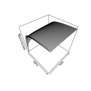
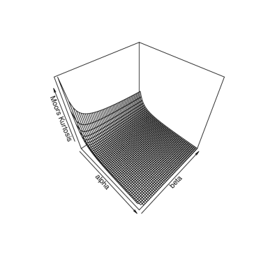
In Figures 3 and 4, we plot the measures B𝐵B and M𝑀M for some parameter values of the EGNH distribution as functions of α𝛼\alpha and β𝛽\beta (for a𝑎a and b𝑏b fixed). These plots indicate that both measures can be very sensitive on these shape parameters and reveal the importance of the proposed distribution.
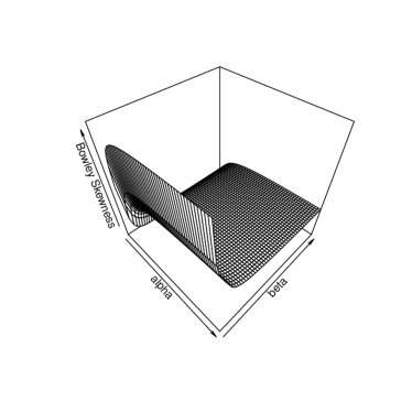
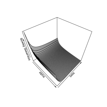
Refer to caption
(a) a=0.5,b=2.0formulae-sequence𝑎0.5𝑏2.0a=0.5,b=2.0
Refer to caption
(b) a=0.5,b=0.5formulae-sequence𝑎0.5𝑏0.5a=0.5,b=0.5
Figure 3: The Bowley skewness of the EGNH distribution as function of α𝛼\alpha and β𝛽\beta.
Refer to caption
(a) a=0.5,b=2.0formulae-sequence𝑎0.5𝑏2.0a=0.5,b=2.0
Refer to caption
(b) a=0.5,b=0.5formulae-sequence𝑎0.5𝑏0.5a=0.5,b=0.5
Figure 4: The Moors kurtosis of the EGNH distribution as function of α𝛼\alpha and β𝛽\beta.

4 Linear Representations

Some useful linear representations for (5) and (6) can be derived using the concept of exponentiated distributions. The properties of these distributions have been studied by many authors in recent years, see Mudholkar and Srivastava (1993) and Mudholkar et al. (1995) for exponentiated Weibull, Gupta et al. (1998) and Gupta and Kundu (2001) for exponentiated exponential, Nadarajah and Gupta (2007) for exponentiated gamma and Cordeiro et al. (2011) for exponentiated generalized gamma distributions. For an arbitrary baseline cdf G(x)𝐺𝑥G(x), a random variable is said to have the exponentiated-G (“exp-G” for short) distribution with power parameter a>0𝑎0a>0, say YexpG(a)similar-to𝑌expG𝑎Y\sim\operatorname{exp-G}(a), if its cdf and pdf are Ha(x)=G(x)asubscript𝐻𝑎𝑥𝐺superscript𝑥𝑎H_{a}(x)=G(x)^{a} and ha(x)=ag(x)G(x)a1subscript𝑎𝑥𝑎𝑔𝑥𝐺superscript𝑥𝑎1h_{a}(x)=ag(x)G(x)^{a-1}, respectively. For any real non-integer β𝛽\beta, we also consider the power series

(1z)β=i=0(1)i(βi)zi,superscript1𝑧𝛽superscriptsubscript𝑖0superscript1𝑖binomial𝛽𝑖superscript𝑧𝑖(1-z)^{\beta}=\sum_{i=0}^{\infty}(-1)^{i}\binom{\beta}{i}z^{i}, (11)

which holds for |z|<1𝑧1|z|<1.

Using expansion (11) in equation (5), we can express the EGNH cdf as

F(x)=i=0(1)i(βi){1[1e1(1+ax)b]}iα𝐹𝑥superscriptsubscript𝑖0superscript1𝑖binomial𝛽𝑖superscript1delimited-[]1superscripte1superscript1𝑎𝑥𝑏𝑖𝛼F(x)=\sum_{i=0}^{\infty}(-1)^{i}\,\binom{\beta}{i}\left\{1-\left[1-\operatorname{\mathrm{e}}^{1-(1+ax)^{b}}\right]\right\}^{i\alpha}

and applying again (11) in the equation above gives

F(x)=i,j=0(1)i+j(βi)(iαj)[1e1(1+ax)b]j.𝐹𝑥superscriptsubscript𝑖𝑗0superscript1𝑖𝑗binomial𝛽𝑖binomial𝑖𝛼𝑗superscriptdelimited-[]1superscripte1superscript1𝑎𝑥𝑏𝑗F(x)=\sum_{i,j=0}^{\infty}(-1)^{i+j}\binom{\beta}{i}\binom{i\alpha}{j}\left[1-\operatorname{\mathrm{e}}^{1-(1+ax)^{b}}\right]^{j}.

Then, the following proposition holds.

Proposition 2.

The EGNH cdf can be rewritten as

F(x)=j=0wjHj(x),𝐹𝑥superscriptsubscript𝑗0subscript𝑤𝑗subscript𝐻𝑗𝑥F(x)=\sum_{j=0}^{\infty}w_{j}\,H_{j}(x), (12)

where the coefficients (for j0𝑗0j\geq 0) are given by

wj=wj(α,β)=i=0(1)i+j(βi)(iαj)subscript𝑤𝑗subscript𝑤𝑗𝛼𝛽superscriptsubscript𝑖0superscript1𝑖𝑗binomial𝛽𝑖binomial𝑖𝛼𝑗w_{j}=w_{j}(\alpha,\beta)=\sum_{i=0}^{\infty}(-1)^{i+j}\binom{\beta}{i}\binom{i\alpha}{j}

and Hj(x)={1exp[1(1+ax)b]}jsubscript𝐻𝑗𝑥superscript11superscript1𝑎𝑥𝑏𝑗H_{j}(x)=\{1-\exp[1-(1+ax)^{b}]\}^{j} is the ENH(j,a,b)𝑗𝑎𝑏(j,a,b) cdf (for j0𝑗0j\geq 0).

We can prove using Mathematica that j=0wj=1superscriptsubscript𝑗0subscript𝑤𝑗1\sum_{j=0}^{\infty}w_{j}=1 as expected.

By differentiating (12), we obtain

f(x)=αβg(x)j=0tjG(x)j𝑓𝑥𝛼𝛽𝑔𝑥superscriptsubscript𝑗0subscript𝑡𝑗𝐺superscript𝑥𝑗f(x)=\alpha\beta g(x)\sum_{j=0}^{\infty}t_{j}\,G(x)^{j} (13)

where the coefficients (for j0𝑗0j\geq 0) are given by

tj=tj(α,β)=i=0(1)i+j(β1i)(α(i+1)1j)subscript𝑡𝑗subscript𝑡𝑗𝛼𝛽superscriptsubscript𝑖0superscript1𝑖𝑗binomial𝛽1𝑖binomial𝛼𝑖11𝑗t_{j}=t_{j}(\alpha,\beta)=\sum_{i=0}^{\infty}(-1)^{i+j}\binom{\beta-1}{i}\binom{\alpha(i+1)-1}{j} (14)

Further, the corollary bellow follows:

Proposition 3.

Equation (13) can be rewritten as

f(x)=j=0ujhj+1(x),𝑓𝑥superscriptsubscript𝑗0subscript𝑢𝑗subscript𝑗1𝑥f(x)=\sum_{j=0}^{\infty}u_{j}\,h_{j+1}(x), (15)

where the coefficients are

uj=uj(α,β)=αβj+1tjsubscript𝑢𝑗subscript𝑢𝑗𝛼𝛽𝛼𝛽𝑗1subscript𝑡𝑗u_{j}=u_{j}(\alpha,\beta)=\frac{\alpha\beta}{j+1}\,t_{j}

and

hj+1(x)=ab(j+1)(1+ax)bexp[1(1+ax)b]{1exp[1(1+ax)b]}jsubscript𝑗1𝑥𝑎𝑏𝑗1superscript1𝑎𝑥𝑏1superscript1𝑎𝑥𝑏superscript11superscript1𝑎𝑥𝑏𝑗h_{j+1}(x)=\frac{ab(j+1)(1+ax)^{b}\exp[1-(1+ax)^{b}]}{\{1-\exp[1-(1+ax)^{b}]\}^{-j}} (16)

is the ENH(j+1,a,b)𝑗1𝑎𝑏(j+1,a,b) pdf.

Equation (15) reveals that the EGNH pdf is an infinite linear combination of ENH pdfs. Thus, some structural properties of the EGNH distribution, such as the ordinary and incomplete moments and generating function, can be determined from those of the ENH model, which have been studied by Lemonte (2013) and Abdul Moniem (2015).

5 Moments

In this section, we derive the moments of the EGNH distribution as well as other related measures. Let YNH(a,b)similar-to𝑌NH𝑎𝑏Y\sim\operatorname{\mathrm{NH}}(a,b) and XEGNH(α,β,a,b)similar-to𝑋EGNH𝛼𝛽𝑎𝑏X\sim\operatorname{\mathrm{EGNH}}(\alpha,\beta,a,b). Cordeiro et al. (2013) proved that the moments of the EG distribution can be expressed as an infinite weighted sum of the (r,j)𝑟𝑗(r,j)th probability weighted moments τr,jsubscript𝜏𝑟𝑗\tau_{r,j} of the baseline random variable. Following this result, we can write from (13)

μr=𝔼(Xr)=αβj=0tjτr,j,superscriptsubscript𝜇𝑟𝔼superscript𝑋𝑟𝛼𝛽superscriptsubscript𝑗0subscript𝑡𝑗subscript𝜏𝑟𝑗\mu_{r}^{\prime}=\operatorname{\mathbb{E}}(X^{r})=\alpha\beta\sum_{j=0}^{\infty}t_{j}\,\tau_{r,j},

where tjsubscript𝑡𝑗t_{j} is given by (14) and

τr,j=𝔼[YrG(Y)j]=xrG(x)jg(x)𝑑x.subscript𝜏𝑟𝑗𝔼superscript𝑌𝑟𝐺superscript𝑌𝑗superscriptsubscriptsuperscript𝑥𝑟𝐺superscript𝑥𝑗𝑔𝑥differential-d𝑥\tau_{r,j}=\operatorname{\mathbb{E}}[Y^{r}\,G(Y)^{j}]=\int_{-\infty}^{\infty}x^{r}\,G(x)^{j}\,g(x)dx.

By simple algebraic manipulations,

τr,j=ab0xr(1+ax)b1exp[1(1+ax)b]{1exp[1(1+ax)b]}j𝑑x.subscript𝜏𝑟𝑗𝑎𝑏superscriptsubscript0superscript𝑥𝑟superscript1𝑎𝑥𝑏11superscript1𝑎𝑥𝑏superscript11superscript1𝑎𝑥𝑏𝑗differential-d𝑥\tau_{r,j}=ab\int_{0}^{\infty}\frac{x^{r}(1+ax)^{b-1}\exp\left[1-(1+ax)^{b}\right]}{\left\{1-\exp\left[1-(1+ax)^{b}\right]\right\}^{-j}}\,dx. (17)

It is clear that |exp[1(1+ax)b]|<11superscript1𝑎𝑥𝑏1\left|\exp\left[1-\left(1+ax\right)^{b}\right]\right|<1, and then applying (11) in (17) gives

τr,j=abk=0(1)k(jk)0xr(1+ax)b1{exp[1(1+ax)b]}k+1𝑑x.subscript𝜏𝑟𝑗𝑎𝑏superscriptsubscript𝑘0superscript1𝑘binomial𝑗𝑘superscriptsubscript0superscript𝑥𝑟superscript1𝑎𝑥𝑏1superscript1superscript1𝑎𝑥𝑏𝑘1differential-d𝑥\tau_{r,j}=ab\,\sum_{k=0}^{\infty}(-1)^{k}\binom{j}{k}\int_{0}^{\infty}x^{r}(1+ax)^{b-1}\left\{\exp\left[1-(1+ax)^{b}\right]\right\}^{k+1}\,dx.

Then, we can write

τr,j=abk=0(1)k(jk)ek+10xr(1+ax)b1exp[(k+1)(1+ax)b]𝑑x.subscript𝜏𝑟𝑗𝑎𝑏superscriptsubscript𝑘0superscript1𝑘binomial𝑗𝑘superscripte𝑘1superscriptsubscript0superscript𝑥𝑟superscript1𝑎𝑥𝑏1𝑘1superscript1𝑎𝑥𝑏differential-d𝑥\tau_{r,j}=ab\,\sum_{k=0}^{\infty}(-1)^{k}\binom{j}{k}\operatorname{\mathrm{e}}^{k+1}\int_{0}^{\infty}x^{r}(1+ax)^{b-1}\exp\left[-(k+1)(1+ax)^{b}\right]\,dx.

By setting y=(k+1)(1+ax)b𝑦𝑘1superscript1𝑎𝑥𝑏y=(k+1)(1+ax)^{b}, τr,jsubscript𝜏𝑟𝑗\tau_{r,j} reduces to

τr,j=1ark=0(1)k+r(jk)ek+1k+1k+1[1(yk+1)1/b]reydy.subscript𝜏𝑟𝑗1superscript𝑎𝑟superscriptsubscript𝑘0superscript1𝑘𝑟binomial𝑗𝑘superscripte𝑘1𝑘1superscriptsubscript𝑘1superscriptdelimited-[]1superscript𝑦𝑘11𝑏𝑟superscripte𝑦𝑑𝑦\tau_{r,j}=\frac{1}{a^{r}}\sum_{k=0}^{\infty}(-1)^{k+r}\binom{j}{k}\frac{\operatorname{\mathrm{e}}^{k+1}}{k+1}\int_{k+1}^{\infty}\left[1-\left(\frac{y}{k+1}\right)^{\nicefrac{{1}}{{b}}}\right]^{r}\operatorname{\mathrm{e}}^{-y}\,dy.

Taking r𝑟r integer and applying the binomial expansion, the last expression becomes

τr,j=1ark=0l=0r(1)k+r+l(jk)(rl)ek+1(k+1)l/b+1Γ(lb+1,k+1),subscript𝜏𝑟𝑗1superscript𝑎𝑟superscriptsubscript𝑘0superscriptsubscript𝑙0𝑟superscript1𝑘𝑟𝑙binomial𝑗𝑘binomial𝑟𝑙superscripte𝑘1superscript𝑘1𝑙𝑏1Γ𝑙𝑏1𝑘1\tau_{r,j}=\frac{1}{a^{r}}\sum_{k=0}^{\infty}\sum_{l=0}^{r}(-1)^{k+r+l}\binom{j}{k}\binom{r}{l}\frac{\operatorname{\mathrm{e}}^{k+1}}{(k+1)^{\nicefrac{{l}}{{b}}+1}}\Gamma\left(\frac{l}{b}+1,k+1\right),

where Γ(a,x)=xya1eydyΓ𝑎𝑥superscriptsubscript𝑥superscript𝑦𝑎1superscripte𝑦𝑑𝑦\Gamma(a,x)=\int_{x}^{\infty}y^{a-1}\operatorname{\mathrm{e}}^{-y}\,dy denotes the complementary incomplete gamma function. Then, the r𝑟rth ordinary moment of X𝑋X is given by

μr=αβarj,k=0l=0r(1)k+r+ltj(jk)(rl)ek+1(k+1)l/b+1Γ(lb+1,k+1).superscriptsubscript𝜇𝑟𝛼𝛽superscript𝑎𝑟superscriptsubscript𝑗𝑘0superscriptsubscript𝑙0𝑟superscript1𝑘𝑟𝑙subscript𝑡𝑗binomial𝑗𝑘binomial𝑟𝑙superscripte𝑘1superscript𝑘1𝑙𝑏1Γ𝑙𝑏1𝑘1\mu_{r}^{\prime}=\frac{\alpha\beta}{a^{r}}\sum_{j,k=0}^{\infty}\sum_{l=0}^{r}(-1)^{k+r+l}\,t_{j}\,\binom{j}{k}\binom{r}{l}\frac{\operatorname{\mathrm{e}}^{k+1}}{(k+1)^{\nicefrac{{l}}{{b}}+1}}\Gamma\left(\frac{l}{b}+1,k+1\right). (18)

For α>0𝛼0\alpha>0 and β>0𝛽0\beta>0 integers, the moments in (18) reduce to

μr=αβarj=0α(i+1)1k=0l=0r(1)k+r+ltj(jk)(rl)ek+1(k+1)l/b+1Γ(lb+1,k+1),superscriptsubscript𝜇𝑟𝛼𝛽superscript𝑎𝑟superscriptsubscript𝑗0𝛼𝑖11superscriptsubscript𝑘0superscriptsubscript𝑙0𝑟superscript1𝑘𝑟𝑙subscript𝑡𝑗binomial𝑗𝑘binomial𝑟𝑙superscripte𝑘1superscript𝑘1𝑙𝑏1Γ𝑙𝑏1𝑘1\mu_{r}^{\prime}=\frac{\alpha\beta}{a^{r}}\sum_{j=0}^{\alpha(i+1)-1}\sum_{k=0}^{\infty}\sum_{l=0}^{r}(-1)^{k+r+l}\,t_{j}\,\binom{j}{k}\binom{r}{l}\frac{\operatorname{\mathrm{e}}^{k+1}}{(k+1)^{\nicefrac{{l}}{{b}}+1}}\Gamma\left(\frac{l}{b}+1,k+1\right),

where tjsubscript𝑡𝑗t_{j} becomes

tj=i=0β1(1)i+j(β1i)(α(i+1)1j).superscriptsubscript𝑡𝑗superscriptsubscript𝑖0𝛽1superscript1𝑖𝑗binomial𝛽1𝑖binomial𝛼𝑖11𝑗t_{j}^{*}=\sum_{i=0}^{\beta-1}(-1)^{i+j}\binom{\beta-1}{i}\binom{\alpha(i+1)-1}{j}.

Additionally, the expression for μrsuperscriptsubscript𝜇𝑟\mu_{r}^{\prime} when α=β=1𝛼𝛽1\alpha=\beta=1 takes the form

μr=earl=0r(1)l+r(rl)Γ(lb+1,1),superscriptsubscript𝜇𝑟esuperscript𝑎𝑟superscriptsubscript𝑙0𝑟superscript1𝑙𝑟binomial𝑟𝑙Γ𝑙𝑏11\mu_{r}^{\prime}=\frac{\operatorname{\mathrm{e}}}{a^{r}}\sum_{l=0}^{r}(-1)^{l+r}\binom{r}{l}\Gamma\left(\frac{l}{b}+1,1\right),

which agrees with the moments given by Nadarajah and Haghighi (2011).

The central moments (μrsubscript𝜇𝑟\mu_{r}) of X𝑋X are given by

μr=m=0r(1)m(rm)μ1mμrm.subscript𝜇𝑟superscriptsubscript𝑚0𝑟superscript1𝑚binomial𝑟𝑚superscriptsubscript𝜇1𝑚superscriptsubscript𝜇𝑟𝑚\mu_{r}=\sum_{m=0}^{r}(-1)^{m}\binom{r}{m}\mu_{1}^{\prime m}\mu_{r-m}^{\prime}. (19)

The cumulants (κrsubscript𝜅𝑟\kappa_{r}), skewness (γ1subscript𝛾1\gamma_{1}) and kurtosis (γ2subscript𝛾2\gamma_{2}) of X𝑋X are determined from (18) using well-known relationships κr=μrm=0r1(r1m1)κmμrmsubscript𝜅𝑟superscriptsubscript𝜇𝑟superscriptsubscript𝑚0𝑟1binomial𝑟1𝑚1subscript𝜅𝑚superscriptsubscript𝜇𝑟𝑚\kappa_{r}=\mu_{r}^{\prime}-\sum_{m=0}^{r-1}\binom{r-1}{m-1}\kappa_{m}\mu_{r-m}^{\prime}, for r1𝑟1r\geq 1, γ1=κ3/κ23/2subscript𝛾1subscript𝜅3superscriptsubscript𝜅232\gamma_{1}=\nicefrac{{\kappa_{3}}}{{\kappa_{2}^{\nicefrac{{3}}{{2}}}}} and γ2=κ4/κ22subscript𝛾2subscript𝜅4superscriptsubscript𝜅22\gamma_{2}=\nicefrac{{\kappa_{4}}}{{\kappa_{2}^{2}}}, where κ1=μ1subscript𝜅1superscriptsubscript𝜇1\kappa_{1}=\mu_{1}^{\prime}.

6 Generating function

The mgf of X𝑋X can be obtained from (15) as

M(s)=j=0ujMj+1(s),𝑀𝑠superscriptsubscript𝑗0subscript𝑢𝑗subscript𝑀𝑗1𝑠\displaystyle M(s)=\sum_{j=0}^{\infty}u_{j}\,M_{j+1}(s),

where Mj+1(s)subscript𝑀𝑗1𝑠M_{j+1}(s) is the mgf of the ENH(j+1,a,b)𝑗1𝑎𝑏(j+1,a,b) distribution (Bourguignon et al., 2015) given by

Mj+1(t)=s,r=0ηsgs,rtj+1r/b+1,subscript𝑀𝑗1𝑡superscriptsubscript𝑠𝑟0subscript𝜂𝑠subscript𝑔𝑠𝑟superscript𝑡𝑗1𝑟𝑏1M_{j+1}(t)=\sum_{s,r=0}^{\infty}\frac{\eta_{s}\,g_{s,r}\,t^{j+1}}{r/b+1}, (20)

where ηi=k=0(1)iλkk!(ki)subscript𝜂𝑖superscriptsubscript𝑘0superscript1𝑖superscript𝜆𝑘𝑘binomial𝑘𝑖\eta_{i}=\sum_{k=0}^{\infty}\frac{(-1)^{i}}{\lambda^{k}k!}\binom{k}{i}, gi,r=(rζ0)1n=1r[n(i+1)r]ζngi,rnsubscript𝑔𝑖𝑟superscript𝑟subscript𝜁01superscriptsubscript𝑛1𝑟delimited-[]𝑛𝑖1𝑟subscript𝜁𝑛subscript𝑔𝑖𝑟𝑛g_{i,r}=(r\zeta_{0})^{-1}\sum_{n=1}^{r}[n(i+1)-r]\zeta_{n}\,g_{i,r-n} for r1𝑟1r\geq 1, gi,0=ζ0isubscript𝑔𝑖0superscriptsubscript𝜁0𝑖g_{i,0}=\zeta_{0}^{i}, ζr=m=0fmdm,rsubscript𝜁𝑟superscriptsubscript𝑚0subscript𝑓𝑚subscript𝑑𝑚𝑟\zeta_{r}=\sum_{m=0}^{\infty}f_{m}\,d_{m,r}, fm=j=m(1)jm(jm)(α1)j/j!subscript𝑓𝑚superscriptsubscript𝑗𝑚superscript1𝑗𝑚binomial𝑗𝑚subscriptsuperscript𝛼1𝑗𝑗f_{m}=\sum_{j=m}^{\infty}(-1)^{j-m}\binom{j}{m}(\alpha^{-1})_{j}/j! and dm,r=(ra0)1v=0r[v(m+1)r]avdm,rvsubscript𝑑𝑚𝑟superscript𝑟subscript𝑎01superscriptsubscript𝑣0𝑟delimited-[]𝑣𝑚1𝑟subscript𝑎𝑣subscript𝑑𝑚𝑟𝑣d_{m,r}=(ra_{0})^{-1}\sum_{v=0}^{r}[v(m+1)-r]\,a_{v}\,d_{m,r-v}. Here, (α1)j=(α1)×(α11)(α1j+1)subscriptsuperscript𝛼1𝑗superscript𝛼1superscript𝛼11superscript𝛼1𝑗1(\alpha^{-1})_{j}=(\alpha^{-1})\times(\alpha^{-1}-1)\ldots(\alpha^{-1}-j+1) is the descending factorial.

7 Mean deviations

The mean deviations about the mean and the median of X𝑋X can be expressed, respectively, as δ1(X)=𝔼(|Xμ1|)=2μ1F(μ1)2m1(μ1)subscript𝛿1𝑋𝔼𝑋superscriptsubscript𝜇12superscriptsubscript𝜇1𝐹superscriptsubscript𝜇12subscript𝑚1superscriptsubscript𝜇1\delta_{1}(X)=\operatorname{\mathbb{E}}(|X-\mu_{1}^{\prime}|)=2\mu_{1}^{\prime}F(\mu_{1}^{\prime})-2m_{1}(\mu_{1}^{\prime}) and δ2(X)=𝔼(|XX~|)=μ12m1(X~)subscript𝛿2𝑋𝔼𝑋~𝑋superscriptsubscript𝜇12subscript𝑚1~𝑋\delta_{2}(X)=\operatorname{\mathbb{E}}(|X-\widetilde{X}|)=\mu_{1}^{\prime}-2m_{1}(\widetilde{X}), where μ1superscriptsubscript𝜇1\mu_{1}^{\prime} comes from (18), F(μ1)𝐹superscriptsubscript𝜇1F(\mu_{1}^{\prime}) is easily calculated from (5) and m1(z)=zxf(x)dxsubscript𝑚1𝑧superscriptsubscript𝑧𝑥𝑓𝑥differential-d𝑥m_{1}(z)=\int_{-\infty}^{z}\!xf(x)\,\mathrm{d}x is the first incomplete moment.

A general equation for m1(z)subscript𝑚1𝑧m_{1}(z) can be derived from (13) as

m1(z)=j=0ujJj+1(z),subscript𝑚1𝑧superscriptsubscript𝑗0subscript𝑢𝑗subscript𝐽𝑗1𝑧m_{1}(z)=\sum_{j=0}^{\infty}u_{j}\,J_{j+1}(z), (21)

where Jj+1(z)=zxhj+1(x)dxsubscript𝐽𝑗1𝑧superscriptsubscript𝑧𝑥subscript𝑗1𝑥differential-d𝑥J_{j+1}(z)=\int_{-\infty}^{z}\!x\,h_{j+1}(x)\,\mathrm{d}x and hj+1(x)subscript𝑗1𝑥h_{j+1}(x) is given by (16). After some algebra, we can prove that

Jj+1(z)=(j+1)ak=0l=01(1)k+l+1ek+1(k+1)1+l+1b(jk)ϕ(a,b,k,l;z),subscript𝐽𝑗1𝑧𝑗1𝑎superscriptsubscript𝑘0superscriptsubscript𝑙01superscript1𝑘𝑙1superscripte𝑘1superscript𝑘11𝑙1𝑏binomial𝑗𝑘italic-ϕ𝑎𝑏𝑘𝑙𝑧J_{j+1}(z)=\frac{(j+1)}{a}\sum_{k=0}^{\infty}\sum_{l=0}^{1}\frac{(-1)^{k+l+1}\operatorname{\mathrm{e}}^{k+1}}{(k+1)^{1+\frac{l+1}{b}}}\,\binom{j}{k}\,\phi(a,b,k,l;z),

where

ϕ(a,b,k,l;z)=γ(b+l+1b,(k+1)(1+az)b)γ(b+l+1b,k+1).italic-ϕ𝑎𝑏𝑘𝑙𝑧𝛾𝑏𝑙1𝑏𝑘1superscript1𝑎𝑧𝑏𝛾𝑏𝑙1𝑏𝑘1\phi(a,b,k,l;z)=\gamma\left(\frac{b+l+1}{b},(k+1)(1+az)^{b}\right)-\gamma\left(\frac{b+l+1}{b},k+1\right).

The Bonferroni and Lorenz curves are defined (for a given probability π𝜋\pi) by B(π)=m1(q)/πμ1𝐵𝜋subscript𝑚1𝑞𝜋superscriptsubscript𝜇1B(\pi)=\nicefrac{{m_{1}(q)}}{{\pi\mu_{1}^{\prime}}} and L(π)=m1(q)/μ1𝐿𝜋subscript𝑚1𝑞superscriptsubscript𝜇1L(\pi)=\nicefrac{{m_{1}(q)}}{{\mu_{1}^{\prime}}}, respectively, where q=Q(π)𝑞𝑄𝜋q=Q(\pi) comes from (7). Using (21), we can easily obtain B(π)𝐵𝜋B(\pi) and L(π)𝐿𝜋L(\pi).

8 Rényi Entropy

The entropy of a random variable X𝑋X with pdf f(x)𝑓𝑥f(x) is a measure of variation of the uncertainty. For any real parameter λ>0𝜆0\lambda>0 and λ1𝜆1\lambda\neq 1, the Rényi entropy is given by

IR(λ)=1(1λ)log(f(x)λdx).subscript𝐼𝑅𝜆11𝜆superscriptsubscript𝑓superscript𝑥𝜆differential-d𝑥I_{R}(\lambda)=\frac{1}{(1-\lambda)}\log\left(\int_{-\infty}^{\infty}\!f(x)^{\lambda}\,\mathrm{d}x\right). (22)

Inserting (3) in equation (22) and, after some algebra, we obtain

IR(λ)=11λ{λlog(abαβ)+αλ+log0(1+ax)λ(b1)exp[αλ(1+ax)b]{1exp[1(1+ax)b]α}λ(1β)dx}.I_{R}(\lambda)=\frac{1}{1-\lambda}\left\{\lambda\log(ab\alpha\beta)+\alpha\lambda+\log\int_{0}^{\infty}\!\frac{(1+ax)^{\lambda(b-1)}\exp\left[-\alpha\lambda\left(1+ax\right)^{b}\right]}{\left\{1-\exp\left[1-\left(1+ax\right)^{b}\right]^{\alpha}\right\}^{\lambda(1-\beta)}}\,\mathrm{d}x\right\}.

Applying the binomial expansion gives

IR(λ)=log(ab)+11λ{λlog(αβ)+αλ+logΣ(α,β,b,λ)},subscript𝐼𝑅𝜆𝑎𝑏11𝜆𝜆𝛼𝛽𝛼𝜆Σ𝛼𝛽𝑏𝜆I_{R}(\lambda)=-\log(ab)+\frac{1}{1-\lambda}\left\{\lambda\log(\alpha\beta)+\alpha\lambda+\log\Sigma(\alpha,\beta,b,\lambda)\right\},

where

Σ(α,β,b,λ)=i=0(λ(β1)i)(1)ieiα[(λ+i)α]λ(b1)+1bΓ(λ(b1)+1b,(λ+i)α).Σ𝛼𝛽𝑏𝜆superscriptsubscript𝑖0binomial𝜆𝛽1𝑖superscript1𝑖superscripte𝑖𝛼superscriptdelimited-[]𝜆𝑖𝛼𝜆𝑏11𝑏Γ𝜆𝑏11𝑏𝜆𝑖𝛼\Sigma(\alpha,\beta,b,\lambda)=\sum_{i=0}^{\infty}\binom{\lambda(\beta-1)}{i}\frac{(-1)^{i}\operatorname{\mathrm{e}}^{i\alpha}}{\left[(\lambda+i)\alpha\right]^{\frac{\lambda(b-1)+1}{b}}}\Gamma\left(\frac{\lambda(b-1)+1}{b},(\lambda+i)\alpha\right). (23)

For β>0𝛽0\beta>0 integer, Equation (23) takes the form

Σ(α,β,b,λ)=i=0β1(λ(β1)i)(1)ieiα[(λ+i)α]λ(b1)+1bΓ(λ(b1)+1b,(λ+i)α).Σ𝛼𝛽𝑏𝜆superscriptsubscript𝑖0𝛽1binomial𝜆𝛽1𝑖superscript1𝑖superscripte𝑖𝛼superscriptdelimited-[]𝜆𝑖𝛼𝜆𝑏11𝑏Γ𝜆𝑏11𝑏𝜆𝑖𝛼\Sigma(\alpha,\beta,b,\lambda)=\sum_{i=0}^{\beta-1}\binom{\lambda(\beta-1)}{i}\frac{(-1)^{i}\operatorname{\mathrm{e}}^{i\alpha}}{\left[(\lambda+i)\alpha\right]^{\frac{\lambda(b-1)+1}{b}}}\Gamma\left(\frac{\lambda(b-1)+1}{b},(\lambda+i)\alpha\right).

For α=β=1𝛼𝛽1\alpha=\beta=1, the expression above reduces to

IR(λ)=log(ab)+11λ{λλ(b1)+1blog(λ)+log[Γ(λ(b1)+1b,λ)]},subscript𝐼𝑅𝜆𝑎𝑏11𝜆𝜆𝜆𝑏11𝑏𝜆Γ𝜆𝑏11𝑏𝜆I_{R}(\lambda)=-\log(ab)+\frac{1}{1-\lambda}\left\{\lambda-\frac{\lambda(b-1)+1}{b}\log(\lambda)+\log\left[\Gamma\left(\frac{\lambda(b-1)+1}{b},\lambda\right)\right]\right\},

which agrees with a result given by Nadarajah and Haghighi (2011).

Figure 5 displays plots of some Rényi entropy curves versus λ𝜆\lambda for the EGNH, ENH and NH distributions with some parameter values. In this case, one can note that the NH entropy is fixed thus, we can measure the impact of the change of α𝛼\alpha and β𝛽\beta additional parameters on the EGNH entropy. This quantity increases when α𝛼\alpha and β𝛽\beta increases with respect the comparison between ENH and EGNH entropies, one can observe that the former is a lower bond of the second and the distance between them is higher when α𝛼\alpha increases.

Refer to caption
(a) α=β=3,a=b=0.5formulae-sequence𝛼𝛽3𝑎𝑏0.5\alpha=\beta=3,a=b=0.5
Refer to caption
(b) α=β=5,a=b=0.5formulae-sequence𝛼𝛽5𝑎𝑏0.5\alpha=\beta=5,a=b=0.5
Refer to caption
(c) α=β=7,a=b=0.5formulae-sequence𝛼𝛽7𝑎𝑏0.5\alpha=\beta=7,a=b=0.5
Figure 5: Rényi entropies curves versus λ𝜆\lambda for the EGNH, ENH and NH distributions

9 Order statistics

The pdf fi:n(x)subscript𝑓:𝑖𝑛𝑥f_{i:n}(x) of the i𝑖ith order statistic, say Xi:nsubscript𝑋:𝑖𝑛X_{i:n}, for i=1,,n𝑖1𝑛i=1,\ldots,n, from independent identically distributed random variables X1,Xnsubscript𝑋1subscript𝑋𝑛X_{1},\ldots X_{n} is given by

fi:n(x)=f(x)B(i,ni+1)F(x)i1[1F(x)]ni.subscript𝑓:𝑖𝑛𝑥𝑓𝑥𝐵𝑖𝑛𝑖1𝐹superscript𝑥𝑖1superscriptdelimited-[]1𝐹𝑥𝑛𝑖f_{i:n}(x)=\frac{f(x)}{B(i,n-i+1)}F(x)^{i-1}\left[1-F(x)\right]^{n-i}.

Following a result given by Cordeiro et al. (2013), the pdf fi:n(x)subscript𝑓:𝑖𝑛𝑥f_{i:n}(x) for the EGNH distribution can be expressed as

fi:n(x)=αβB(i,ni)l=0slhl+1(x),subscript𝑓:𝑖𝑛𝑥𝛼𝛽𝐵𝑖𝑛𝑖superscriptsubscript𝑙0subscript𝑠𝑙subscript𝑙1𝑥f_{i:n}(x)=\frac{\alpha\beta}{B(i,n-i)}\sum_{l=0}^{\infty}\,s_{l}\,h_{l+1}(x), (24)

where

sl=j=0nik=0(1)j+k+l(nij)(β(j+1)1k)(α(k+1)1l)subscript𝑠𝑙superscriptsubscript𝑗0𝑛𝑖superscriptsubscript𝑘0superscript1𝑗𝑘𝑙binomial𝑛𝑖𝑗binomial𝛽𝑗11𝑘binomial𝛼𝑘11𝑙s_{l}=\sum_{j=0}^{n-i}\sum_{k=0}^{\infty}(-1)^{j+k+l}\binom{n-i}{j}\binom{\beta(j+1)-1}{k}\binom{\alpha(k+1)-1}{l}

and hl+1(x)subscript𝑙1𝑥h_{l+1}(x) is the ENH(l+1,a,b)𝑙1𝑎𝑏(l+1,a,b) pdf given by (16).

Equation (24) reveals that the pdf of the EGNH order statistic is a linear combination of ENH densities. A direct application of this expansion allows us to determine the ordinary moments and the mgf of the EGNH order statistics.

The r𝑟rth ordinary moment of Xi:nsubscript𝑋:𝑖𝑛X_{i:n} is given by

𝔼(Xi:nr)=αβB(i,ni+1)l=0sl0xrhl+1(x)dx.𝔼subscriptsuperscript𝑋𝑟:𝑖𝑛𝛼𝛽𝐵𝑖𝑛𝑖1superscriptsubscript𝑙0subscript𝑠𝑙superscriptsubscript0superscript𝑥𝑟subscript𝑙1𝑥differential-d𝑥\operatorname{\mathbb{E}}(X^{r}_{i:n})=\frac{\alpha\beta}{B(i,n-i+1)}\sum_{l=0}^{\infty}s_{l}\,\int_{0}^{\infty}\!x^{r}\,h_{l+1}(x)\,\mathrm{d}x. (25)

Equation (25) reveals that the moments of the order statistics depend on the moments of the ENH(l+1,a,b)𝑙1𝑎𝑏(l+1,a,b) distribution. Lemonte (2013) determined the moments of the ENH distribution as

μr=βarm=0rp=0(rm)(β1p)(1)rm+pep+1(p+1)mb+1Γ(mb+1,p+1).superscriptsubscript𝜇𝑟𝛽superscript𝑎𝑟superscriptsubscript𝑚0𝑟superscriptsubscript𝑝0binomial𝑟𝑚binomial𝛽1𝑝superscript1𝑟𝑚𝑝superscripte𝑝1superscript𝑝1𝑚𝑏1Γ𝑚𝑏1𝑝1\mu_{r}^{\prime}=\frac{\beta}{a^{r}}\sum_{m=0}^{r}\sum_{p=0}^{\infty}\binom{r}{m}\binom{\beta-1}{p}\frac{(-1)^{r-m+p}\operatorname{\mathrm{e}}^{p+1}}{(p+1)^{\frac{m}{b}+1}}\Gamma\left(\frac{m}{b}+1,p+1\right).

From this result, Equation (25) can be reduced to

𝔼(Xi:nr)=αβ2B(i,ni+1)l=0slΓ(mb+1,t+1),𝔼subscriptsuperscript𝑋𝑟:𝑖𝑛𝛼superscript𝛽2𝐵𝑖𝑛𝑖1superscriptsubscript𝑙0subscriptsuperscript𝑠𝑙Γ𝑚𝑏1𝑡1\operatorname{\mathbb{E}}(X^{r}_{i:n})=\frac{\alpha\beta^{2}}{B(i,n-i+1)}\sum_{l=0}^{\infty}s^{*}_{l}\,\Gamma\left(\frac{m}{b}+1,t+1\right),

where

sl=m=0rp=0sl(rm)(β1p)(1)rm+pep+1ar(p+1)mb+1.subscriptsuperscript𝑠𝑙superscriptsubscript𝑚0𝑟superscriptsubscript𝑝0subscript𝑠𝑙binomial𝑟𝑚binomial𝛽1𝑝superscript1𝑟𝑚𝑝superscripte𝑝1superscript𝑎𝑟superscript𝑝1𝑚𝑏1s^{*}_{l}=\sum_{m=0}^{r}\sum_{p=0}^{\infty}s_{l}\,\binom{r}{m}\binom{\beta-1}{p}\frac{(-1)^{r-m+p}\operatorname{\mathrm{e}}^{p+1}}{a^{r}(p+1)^{\frac{m}{b}+1}}.

Further, the mgf of Xi:nsubscript𝑋:𝑖𝑛X_{i:n} can follow from (24) as

M(t)=αβB(i,ni+1)l=0sl0etxhl+1(x)dx=αβB(i,ni+1)l=0slMl+1(t),𝑀𝑡𝛼𝛽𝐵𝑖𝑛𝑖1superscriptsubscript𝑙0subscript𝑠𝑙superscriptsubscript0superscripte𝑡𝑥subscript𝑙1𝑥differential-d𝑥𝛼𝛽𝐵𝑖𝑛𝑖1superscriptsubscript𝑙0subscript𝑠𝑙subscript𝑀𝑙1𝑡M(t)=\frac{\alpha\beta}{B(i,n-i+1)}\sum_{l=0}^{\infty}s_{l}\,\int_{0}^{\infty}\operatorname{\mathrm{e}}^{tx}\,h_{l+1}(x)\,\mathrm{d}x=\frac{\alpha\beta}{B(i,n-i+1)}\sum_{l=0}^{\infty}s_{l}\,M_{l+1}(t),

where Ml+1(t)subscript𝑀𝑙1𝑡M_{l+1}(t) is given by (20).

10 Maximum likelihood estimation

In this section, we provide an analytic procedure to obtain the MLEs for the EGNH parameters using the profile log-likelihood function (pllf). The MLEs are employed due to their interesting asymptotic properties. By means of such properties, one can construct confidence intervals for the model parameters.

Let X be the EGNH distribution with vector of parameters 𝜽=(α,β,a,b)𝜽superscript𝛼𝛽𝑎𝑏top\bm{\theta}=(\alpha,\beta,a,b)^{\top}. The log-likelihood function for 𝜽𝜽\bm{\theta}, given the observed sample x1,,xnsubscript𝑥1subscript𝑥𝑛x_{1},\ldots,x_{n}, due to (6) is given by

(𝜽)=n[α+log(aαbβ)]+(b1)i=1nlog(axi+1)αi=1n(axi+1)b+(β1)i=1nlog{1[e1(axi+1)b]α}.𝜽𝑛delimited-[]𝛼𝑎𝛼𝑏𝛽𝑏1superscriptsubscript𝑖1𝑛𝑎subscript𝑥𝑖1𝛼superscriptsubscript𝑖1𝑛superscript𝑎subscript𝑥𝑖1𝑏𝛽1superscriptsubscript𝑖1𝑛1superscriptdelimited-[]superscripte1superscript𝑎subscript𝑥𝑖1𝑏𝛼\begin{split}\ell(\bm{\theta})=&n[\alpha+\log(a\alpha b\beta)]+(b-1)\sum_{i=1}^{n}\log(ax_{i}+1)-\alpha\sum_{i=1}^{n}(ax_{i}+1)^{b}\\ &+(\beta-1)\sum_{i=1}^{n}\log\left\{1-\left[\operatorname{\mathrm{e}}^{1-(ax_{i}+1)^{b}}\right]^{\alpha}\right\}.\end{split} (26)

The components of the associated score vector U=(α,β,a,b)Usuperscript𝛼𝛽𝑎𝑏top\textbf{U}=\left(\frac{\partial\ell}{\partial\alpha},\frac{\partial\ell}{\partial\beta},\frac{\partial\ell}{\partial a},\frac{\partial\ell}{\partial b}\right)^{\top} are

(𝜽)α=𝜽𝛼absent\displaystyle\frac{\partial\ell(\bm{\theta})}{\partial\alpha}= nα+i=1n[1(1+axi)b]{1(β1){exp[1(1+axi)b]}α1{exp[1(1+axi)b]}α},𝑛𝛼superscriptsubscript𝑖1𝑛delimited-[]1superscript1𝑎subscript𝑥𝑖𝑏1𝛽1superscript1superscript1𝑎subscript𝑥𝑖𝑏𝛼1superscript1superscript1𝑎subscript𝑥𝑖𝑏𝛼\displaystyle\frac{n}{\alpha}+\sum\limits_{i=1}^{n}\left[1-(1+ax_{i})^{b}\right]\left\{1-\frac{(\beta-1)\{\exp\left[1-(1+ax_{i})^{b}\right]\}^{\alpha}}{1-\left\{\exp\left[1-(1+ax_{i})^{b}\right]\right\}^{\alpha}}\right\},
(𝜽)β=𝜽𝛽absent\displaystyle\frac{\partial\ell(\bm{\theta})}{\partial\beta}= nβ+i=1nlog{1{exp[1(1+axi)b]}α},𝑛𝛽superscriptsubscript𝑖1𝑛1superscript1superscript1𝑎subscript𝑥𝑖𝑏𝛼\displaystyle\frac{n}{\beta}+\sum\limits_{i=1}^{n}\log\left\{1-\left\{\exp\left[1-(1+ax_{i})^{b}\right]\right\}^{\alpha}\right\}, (27)
(𝜽)a=𝜽𝑎absent\displaystyle\frac{\partial\ell(\bm{\theta})}{\partial a}= na+(b1)i=1nxi1+axiαi=1n[bxi(1+axi)b1]𝑛𝑎𝑏1superscriptsubscript𝑖1𝑛subscript𝑥𝑖1𝑎subscript𝑥𝑖𝛼superscriptsubscript𝑖1𝑛delimited-[]𝑏subscript𝑥𝑖superscript1𝑎subscript𝑥𝑖𝑏1\displaystyle\frac{n}{a}+(b-1)\sum\limits_{i=1}^{n}\frac{x_{i}}{1+ax_{i}}-\alpha\sum\limits_{i=1}^{n}\left[bx_{i}(1+ax_{i})^{b-1}\right]
+α(β1)i=1nbxi(1+axi)b1exp{α[1(1+axi)b]}1{exp[1(1+axi)b]}α,𝛼𝛽1superscriptsubscript𝑖1𝑛𝑏subscript𝑥𝑖superscript1𝑎subscript𝑥𝑖𝑏1𝛼delimited-[]1superscript1𝑎subscript𝑥𝑖𝑏1superscript1superscript1𝑎subscript𝑥𝑖𝑏𝛼\displaystyle+\alpha(\beta-1)\sum\limits_{i=1}^{n}\frac{bx_{i}(1+ax_{i})^{b-1}\exp\left\{\alpha\left[1-(1+ax_{i})^{b}\right]\right\}}{1-\{\exp\left[1-(1+ax_{i})^{b}\right]\}^{\alpha}},

and

(𝜽)b=𝜽𝑏absent\displaystyle\frac{\partial\ell(\bm{\theta})}{\partial b}= nb+i=1nlog(1+axi)αi=1n{[log(1+axi)](1+axi)b}𝑛𝑏superscriptsubscript𝑖1𝑛1𝑎subscript𝑥𝑖𝛼superscriptsubscript𝑖1𝑛delimited-[]1𝑎subscript𝑥𝑖superscript1𝑎subscript𝑥𝑖𝑏\displaystyle\frac{n}{b}+\sum\limits_{i=1}^{n}\log(1+ax_{i})-\alpha\sum\limits_{i=1}^{n}\left\{\left[\log(1+ax_{i})\right](1+ax_{i})^{b}\right\}
+α(β1)i=1n[log(1+axi)](1+axi)bexp{α[1(1+axi)b]}1{exp[1(1+axi)b]}α.𝛼𝛽1superscriptsubscript𝑖1𝑛delimited-[]1𝑎subscript𝑥𝑖superscript1𝑎subscript𝑥𝑖𝑏𝛼delimited-[]1superscript1𝑎subscript𝑥𝑖𝑏1superscript1superscript1𝑎subscript𝑥𝑖𝑏𝛼\displaystyle+\alpha(\beta-1)\sum\limits_{i=1}^{n}\frac{\left[\log(1+ax_{i})\right](1+ax_{i})^{b}\exp\left\{\alpha\left[1-(1+ax_{i})^{b}\right]\right\}}{1-\{\exp\left[1-(1+ax_{i})^{b}\right]\}^{\alpha}}.

The MLEs, 𝜽^=(α^,β^,a^,b^)bold-^𝜽superscript^𝛼^𝛽^𝑎^𝑏top\bm{\hat{\theta}}=(\hat{\alpha},\hat{\beta},\hat{a},\hat{b})^{\top}, can be obtained numerically by solving the system of nonlinear equations

(𝜽)α=(𝜽)β=(𝜽)a=(𝜽)b=0.𝜽𝛼𝜽𝛽𝜽𝑎𝜽𝑏0\frac{\partial\ell(\bm{\theta})}{\partial\alpha}=\frac{\partial\ell(\bm{\theta})}{\partial\beta}=\frac{\partial\ell(\bm{\theta})}{\partial a}=\frac{\partial\ell(\bm{\theta})}{\partial b}=0.

Note that from (27) it is possible to obtain a semi-closed estimator of β𝛽\beta. From (𝜽)β=0𝜽𝛽0\frac{\partial\ell(\bm{\theta})}{\partial\beta}=0, the estimator for β𝛽\beta is given by

β^(α^,a^,b^)=ni=1nlog{1{exp[1(1+a^xi)b^]}α^}.^𝛽^𝛼^𝑎^𝑏𝑛superscriptsubscript𝑖1𝑛1superscript1superscript1^𝑎subscript𝑥𝑖^𝑏^𝛼\hat{\beta}(\hat{\alpha},\hat{a},\hat{b})=-\frac{n}{\sum\limits_{i=1}^{n}\log\left\{1-\left\{\exp\left[1-(1+\hat{a}x_{i})^{\hat{b}}\right]\right\}^{\hat{\alpha}}\right\}}. (28)

Based on (28), fixed on x1,,xnsubscript𝑥1subscript𝑥𝑛x_{1},\ldots,x_{n}, β^0^+^𝛽superscript^0\hat{\beta}\to\hat{0}^{+} when b^0^+^𝑏superscript^0\hat{b}\to\hat{0}^{+} and/or α^0^+^𝛼superscript^0\hat{\alpha}\to\hat{0}^{+}. This behavior anticipates that estimates for smaller α𝛼\alpha and/or b𝑏b may require improved estimation procedures.

Another way to obtain the MLEs is using the pllf. We suppose β𝛽\beta fixed and rewrite (26) as (𝜽)=β(α,a,b)𝜽subscript𝛽𝛼𝑎𝑏\ell(\bm{\theta})=\ell_{\beta}(\alpha,a,b) (to show that β𝛽\beta is fixed but 𝜽β=(α,a,b)subscript𝜽𝛽superscript𝛼𝑎𝑏top\bm{\theta}_{\beta}=(\alpha,a,b)^{\top} varies). To estimate 𝜽βsubscript𝜽𝛽\bm{\theta}_{\beta}, we maximize β(α,a,b)subscript𝛽𝛼𝑎𝑏\ell_{\beta}(\alpha,a,b) with respect to 𝜽βsubscript𝜽𝛽\bm{\theta}_{\beta}, i.e.,

𝜽^β=argmax𝜽ββ(α,a,b).subscriptbold-^𝜽𝛽subscriptsubscript𝜽𝛽subscript𝛽𝛼𝑎𝑏\bm{\hat{\theta}}_{\beta}=\arg\max_{\bm{\theta}_{\beta}}\ell_{\beta}(\alpha,a,b).

By replacing β𝛽\beta by β^(α,a,b)^𝛽𝛼𝑎𝑏\hat{\beta}(\alpha,a,b) in (26), we can obtain the pllf for α𝛼\alpha, a𝑎a and b𝑏b as

β(α,a,b)=subscript𝛽𝛼𝑎𝑏absent\displaystyle\ell_{\beta}(\alpha,a,b)= {α+log{αnabi=1nlog[1(e1(axi+1)b)α]}}𝛼𝛼𝑛𝑎𝑏superscriptsubscript𝑖1𝑛1superscriptsuperscripte1superscript𝑎subscript𝑥𝑖1𝑏𝛼\displaystyle\left\{\alpha+\log\left\{\alpha-{\frac{nab}{\sum_{i=1}^{n}\log\left[1-\left({{\rm e}^{1-\left(ax_{{i}}+1\right)^{b}}}\right)^{\alpha}\right]}}\right\}\right\}
+(b1)i=1nlog(axi+1)αi=1n(axi+1)b𝑏1superscriptsubscript𝑖1𝑛𝑎subscript𝑥𝑖1𝛼superscriptsubscript𝑖1𝑛superscript𝑎subscript𝑥𝑖1𝑏\displaystyle+\left(b-1\right)\sum_{i=1}^{n}\log\left(ax_{{i}}+1\right)-\alpha\,\sum_{i=1}^{n}\left(ax_{{i}}+1\right)^{b}
{ni=1nlog[1(e1(axi+1)b)α]+1}i=1nlog{1[e1(axi+1)b]α}.𝑛superscriptsubscript𝑖1𝑛1superscriptsuperscripte1superscript𝑎subscript𝑥𝑖1𝑏𝛼1superscriptsubscript𝑖1𝑛1superscriptdelimited-[]superscripte1superscript𝑎subscript𝑥𝑖1𝑏𝛼\displaystyle-\left\{{\frac{n}{\sum_{i=1}^{n}\log\left[1-\left({{\rm e}^{1-\left(ax_{{i}}+1\right)^{b}}}\right)^{\alpha}\right]}}+1\right\}\sum_{i=1}^{n}\log\left\{1-\left[{{\rm e}^{1-\left(ax_{{i}}+1\right)^{b}}}\right]^{\alpha}\right\}. (29)

As a consequence MLEs for α𝛼\alpha, a𝑎a and b𝑏b can also be determined by maximizing the pllf (10) with respect to these parameters. Another way to obtain the MLEs is to solve the profile log-likelihood equations

β(α,a,b)α=β(α,a,b)a=β(α,a,b)b=0.subscript𝛽𝛼𝑎𝑏𝛼subscript𝛽𝛼𝑎𝑏𝑎subscript𝛽𝛼𝑎𝑏𝑏0\displaystyle\frac{\partial\ell_{\beta}(\alpha,a,b)}{\partial\alpha}=\frac{\partial\ell_{\beta}(\alpha,a,b)}{\partial a}=\frac{\partial\ell_{\beta}(\alpha,a,b)}{\partial b}=0.

It should be noted that the maximization of (10) is simpler than the maximization of (26) with respect to their respective parameters, since the pllf has three parameters, whereas the llf has four parameters.

For interval estimation on the model parameters, we require the 4×4444\times 4 observed information matrix, J(θ)𝐽𝜃J(\theta), whose elements.

Under standard regularity conditions, the asymptotic distribution of n(𝜽^𝜽)𝑛bold-^𝜽𝜽\sqrt{n}(\bm{\hat{\theta}}-\bm{\theta}) is multivariate normal N4(0,I(𝜽)1)subscript𝑁40𝐼superscript𝜽1N_{4}(0,I(\bm{\theta})^{-1}), where I(𝜽)𝐼𝜽I(\bm{\theta}) is the expected information matrix. This approximated distribution holds when I(𝜽)𝐼𝜽I(\bm{\theta}) is replaced by J(𝜽)𝐽𝜽J(\bm{\theta}). The multivariate normal N4(0,J(𝜽)1)subscript𝑁40𝐽superscript𝜽1N_{4}(0,J(\bm{\theta})^{-1}) distribution for n(𝜽^𝜽)𝑛bold-^𝜽𝜽\sqrt{n}(\bm{\hat{\theta}}-\bm{\theta}) can be used to construct approximate confidence intervals for the individual parameters.

11 Simulation studies

In this section, we assess the performance of the MLEs for α𝛼\alpha, β𝛽\beta, a𝑎a and b𝑏b by means of a Monte Carlo study. To that end, we adopt sample sizes n{10,15,,250}𝑛1015250n\in\{10,15,\ldots,250\} and the parameter values 𝜽=(α,β,a,b)=(1.8×103,2.83×101,1.75×103,47.066)𝜽𝛼𝛽𝑎𝑏1.8superscript1032.83superscript1011.75superscript10347.066\bm{\theta}=(\alpha,\beta,a,b)=(1.8\times 10^{-3},2.83\times 10^{-1},1.75\times 10^{-3},47.066) (defined from the first application to real data discussed in Section 12).

Our simulation study consists of the following steps. For each pair (𝜽,n)𝜽𝑛(\bm{\theta},n), with 𝜽=(α,β,a,b)𝜽𝛼𝛽𝑎𝑏\bm{\theta}=(\alpha,\beta,a,b):

  1. 1.

    generate n𝑛n outcomes of the EGNH distribution;

  2. 2.

    obtain the MLEs;

  3. 3.

    compute the average biases and standard errors.

The simulation study is performed using the R programming language and the BFGS (constrained) method. For maximizing the pllf (10), we use the MaxLik package (Henningsen and Toomet, 2011).

Figures 6 and 7 display results of this simulation study. As expected, both biases and standard errors decrease when the sample size increases. This proposed estimation procedure can be used effectively for estimating the parameters of the EGNH family. Further, it is important to note that the estimate for β𝛽\beta are good, even before the small value considered of α𝛼\alpha.

Refer to caption
Figure 6: Std. errors of the estimates vs. sample size for (α,β,a,b)=(1.8×103,2.83×101,1.75×103,47.066)𝛼𝛽𝑎𝑏1.8superscript1032.83superscript1011.75superscript10347.066(\alpha,\beta,a,b)=(1.8\times 10^{-3},2.83\times 10^{-1},1.75\times 10^{-3},47.066)
Refer to caption
Figure 7: Biases of the estimates vs. sample size for (α,β,a,b)=(1.8×103,2.83×101,1.75×103,47.066)𝛼𝛽𝑎𝑏1.8superscript1032.83superscript1011.75superscript10347.066(\alpha,\beta,a,b)=(1.8\times 10^{-3},2.83\times 10^{-1},1.75\times 10^{-3},47.066)

12 Applications

Figure 8: TTT-plots of datasets

In this section, we present two applications to real data in order to illustrate the EGNH potentiality. The first uncensored real dataset refers to the lifetimes of 50 components (Aarset, 1987): 0.1, 7, 36, 67, 84, 0.2, 11, 40, 67, 84, 1, 12, 45, 67, 84, 1, 18, 46, 67, 85, 1, 18, 47, 72, 85, 1, 18, 50, 75, 85, 1, 18, 55, 79, 85, 2, 18, 60, 82, 85, 3, 21, 63, 82, 86, 6, 32, 63, 83, 86. The second uncensored dataset represents the stress-rupture life of kevlar 49/epoxy strands, which were subjected to constant sustained pressure at 70% stress level until all units had failed (Andrews and Herzberg, 1985): 1051, 1337, 1389, 1921, 1942, 2322, 3629, 4006, 4012, 4063, 4921, 5445, 5620, 5817, 5905, 5956, 6068, 6121, 6473, 7501, 7886, 8108, 8546, 8666, 8831, 9106, 9711, 9806, 10205, 10396, 10861, 11026, 11214, 11362, 11604, 11608, 11745, 11762, 11895, 12044, 13520, 13670, 14110, 14496, 15395, 16179, 17092, 17568, 17568. For a previous study with this dataset, see Cooray and Ananda (2008).

Table 3 gives a descriptive summary of the two samples. For both datasets, the median is greater than the mean (indicating asymmetry). The Aarset dataset has negative skewness (left-skewed data), while the Andrews and Herzberg dataset has positive one (right-skewed data).

Table 3: Descriptive Statistics
Datasets Mean Median Variance Skew. Kurt. Min. Max.
Aarset 45.686 48.5 1078.153 -0.1378 1.414 0.1 86
Andrews and Herzberg 8805.694 8831 20738145 0.097 2.172 1051 17568

In many applications empirical hrf shape can indicate a particular model. The plot of total time on test (TTT) (Aarset, 1987) can be useful in this sense. The TTT plot is obtained by plotting G(r/n)=(i=1ryi:n+(nr)yr:n)/i=1nyi:n𝐺𝑟𝑛superscriptsubscript𝑖1𝑟subscript𝑦:𝑖𝑛𝑛𝑟subscript𝑦:𝑟𝑛superscriptsubscript𝑖1𝑛subscript𝑦:𝑖𝑛G(r/n)=\nicefrac{{(\sum_{i=1}^{r}y_{i:n}+(n-r)y_{r:n})}}{{\sum_{i=1}^{n}y_{i:n}}}, where r=1,,n𝑟1𝑛r=1,\ldots,n and yi:n(i=1,,n)subscript𝑦:𝑖𝑛𝑖1𝑛y_{i:n}(i=1,\ldots,n) are the order statistics of the sample, against r/n𝑟𝑛r/n. The TTT plots for the current datasets are presented in Figure 8. The TTT plot for the Aarset’s data indicates a bathtub-shaped hrf and the TTT plot for the Andrews and Herzberg’s data indicates an increasing hrf. Therefore, these plots reveal the appropriateness of the EGNH distribution to fit these datasets, since the new model can present bathtub-shaped and increasing hrfs.

We compare the fits of the EGNH distribution defined in (6) with the submodels NH, EE and ENH and additionally with some other lifetime models with four, three and two parameters, namely:

  • The Kumaraswamy Nadarajah-Haghighi (KNH) distribution (Lima, 2015) having pdf (for x>0𝑥0x>0) given by

    fKNH(x)=abαβ(1+ax)bexp[1(1+ax)b]{1exp[1(1+ax)b]}α1{1{1exp[1(1+ax)b]}α}1β.subscript𝑓𝐾𝑁𝐻𝑥𝑎𝑏𝛼𝛽superscript1𝑎𝑥𝑏1superscript1𝑎𝑥𝑏superscript11superscript1𝑎𝑥𝑏𝛼1superscript1superscript11superscript1𝑎𝑥𝑏𝛼1𝛽\displaystyle f_{KNH}(x)=\frac{ab\alpha\beta(1+ax)^{b}\exp\left[1-(1+ax)^{b}\right]\left\{1-\exp\left[1-(1+ax)^{b}\right]\right\}^{\alpha-1}}{\left\{1-\left\{1-\exp\left[1-\left(1+ax\right)^{b}\right]\right\}^{\alpha}\right\}^{1-\beta}}.
  • The beta Nadarajah-Haghighi (BNH) distribution (Dias, 2016) having pdf (for x>0𝑥0x>0) given by

    fBNH(x)=abB(α,β)(1+ax)b1{1exp[1(1+ax)b]}α1{exp[1(1+ax)b]}β.subscript𝑓𝐵𝑁𝐻𝑥𝑎𝑏𝐵𝛼𝛽superscript1𝑎𝑥𝑏1superscript11superscript1𝑎𝑥𝑏𝛼1superscript1superscript1𝑎𝑥𝑏𝛽\displaystyle f_{BNH}(x)=\frac{ab}{B(\alpha,\beta)}(1+ax)^{b-1}\left\{1-\exp\left[1-(1+ax)^{b}\right]\right\}^{\alpha-1}\left\{\exp\left[1-(1+ax)^{b}\right]\right\}^{\beta}.
  • The Zografos-Balakrishnan Nadarajah-Haghighi (ZBNH) distribution (Bourguignon et al., 2015) having pdf (for x>0𝑥0x>0) given by

    fZBNH(x)=abΓ(α)(1+ax)b[(1+ax)b1]α1exp{[(1+ax)b1]}.subscript𝑓𝑍𝐵𝑁𝐻𝑥𝑎𝑏Γ𝛼superscript1𝑎𝑥𝑏superscriptdelimited-[]superscript1𝑎𝑥𝑏1𝛼1delimited-[]superscript1𝑎𝑥𝑏1\displaystyle f_{ZBNH}(x)=\frac{ab}{\Gamma(\alpha)}(1+ax)^{b}\left[\left(1+ax\right)^{b}-1\right]^{\alpha-1}\exp\left\{-\left[\left(1+ax\right)^{b}-1\right]\right\}.
  • The Marshall-Olkin Nadarajah-Haghighi (MONH) distribution (Lemonte et al., 2016) having pdf (for x>0𝑥0x>0) given by

    fMONH(x)=abα(1+ax)b1exp[1(1+ax)b]{1(1α)exp[1(1+ax)b]}2.subscript𝑓𝑀𝑂𝑁𝐻𝑥𝑎𝑏𝛼superscript1𝑎𝑥𝑏11superscript1𝑎𝑥𝑏superscript11𝛼1superscript1𝑎𝑥𝑏2\displaystyle f_{MONH}(x)=\frac{ab\alpha(1+ax)^{b-1}\exp\left[1-\left(1+ax\right)^{b}\right]}{\left\{1-\left(1-\alpha\right)\exp\left[1-\left(1+ax\right)^{b}\right]\right\}^{2}}.
  • The transmuted Nadarajah-Haghighi (TNH) distribution (Ahmed et al., 2015) having pdf (for x>0𝑥0x>0) given by

    fTNH(x)=ab(1+ax)b1exp[1(1+ax)b]{(1α)+2αexp[1(1+ax)b]}.subscript𝑓𝑇𝑁𝐻𝑥𝑎𝑏superscript1𝑎𝑥𝑏11superscript1𝑎𝑥𝑏1𝛼2𝛼1superscript1𝑎𝑥𝑏\displaystyle f_{TNH}(x)=ab(1+ax)^{b-1}\exp\left[1-\left(1+ax\right)^{b}\right]\left\{\left(1-\alpha\right)+2\alpha\exp\left[1-\left(1+ax\right)^{b}\right]\right\}.
  • The modified Nadarajah-Haghighi (MNH) distribution (El Damcese and Ramadan, 2015) having pdf (for x>0𝑥0x>0) given by

    fMNH(x)=α(λ+2βx)(1+λx+βx2)α1exp[1(1+λx+βx2)α].subscript𝑓𝑀𝑁𝐻𝑥𝛼𝜆2𝛽𝑥superscript1𝜆𝑥𝛽superscript𝑥2𝛼11superscript1𝜆𝑥𝛽superscript𝑥2𝛼\displaystyle f_{MNH}(x)=\alpha(\lambda+2\beta x)(1+\lambda x+\beta x^{2})^{\alpha-1}\exp\left[1-\left(1+\lambda x+\beta x^{2}\right)^{\alpha}\right].
  • The generalized power Weibull (GPW) distribution (Nikulin and Haghighi, 2006) having pdf (for x>0𝑥0x>0) given by

    fGPW(x)=abcxc1(1+axc)b1exp[1(1+axc)b].subscript𝑓𝐺𝑃𝑊𝑥𝑎𝑏𝑐superscript𝑥𝑐1superscript1𝑎superscript𝑥𝑐𝑏11superscript1𝑎superscript𝑥𝑐𝑏\displaystyle f_{GPW}(x)=abcx^{c-1}\left(1+a{x}^{c}\right)^{b-1}\exp[1-\left(1+a{x}^{c}\right)^{b}].
  • The classic Weibull distribution having pdf (for x>0𝑥0x>0) given by

    fWeibull(x)=(ab)(xb)a1exp[(xb)a].subscript𝑓𝑊𝑒𝑖𝑏𝑢𝑙𝑙𝑥𝑎𝑏superscript𝑥𝑏𝑎1superscript𝑥𝑏𝑎\displaystyle f_{Weibull}(x)=\left(\frac{a}{b}\right)\left(\frac{x}{b}\right)^{a-1}\exp\left[-\left(\frac{x}{b}\right)^{a}\right].

Tables 4 and 5 present the MLEs and their standard errors for some models fitted to the Aarset’s and Andrews and Herzberg’s datasets, respectively. In order to compare the competitive models, Tables 6 and 7 list the Goodness-of-Fit (GoF) statistics of the fitted models for the Aarset’s and Andrews and Herzberg’s datasets, respectively. We use the following GoF statistics: Cramér-von Mises (W*), Anderson Darling (A*), Kolmogorov-Smirnov (KS), Akaike Information Criterion (AIC), Bayesian Information Criterion (BIC), Consistent Akaike Information Criterion (CAIC) and Hannan-Quinn Information Criterion (HQIC). They are used to verify the quality of the fits. In general, smaller GoF values are associated with better fits.

Table 4: Estimates for Aarset’s dataset
model estimates
EGNH(α,β,a,b)EGNH𝛼𝛽𝑎𝑏\operatorname{\mathrm{EGNH}}(\alpha,\beta,a,b) 1.8×1031.8superscript1031.8\times 10^{-3} 2.83×1012.83superscript1012.83\times 10^{-1} 1.75×1031.75superscript1031.75\times 10^{-3} 47.066
(8.8×10⁴)8.8superscript104(8.8\times 10^{-4}) (1.19×10²)1.19superscript102(1.19\times 10^{-2}) (2.47×10⁴)2.47superscript104(2.47\times 10^{-4}) (3.69)3.69(3.69)
BNH(α,β,a,b)𝛼𝛽𝑎𝑏(\alpha,\beta,a,b) 2.55×1012.55superscript1012.55\times 10^{-1} (5.2×10²)5.2superscript102(5.2\times 10^{-2}) 5.225×1035.225superscript1035.225\times 10^{-3} 9.753
(2.41×10²)2.41superscript102(2.41\times 10^{-2}) (1.93×10²)1.93superscript102(1.93\times 10^{-2}) (5.018×10⁴)5.018superscript104(5.018\times 10^{-4}) (3.20)3.20(3.20)
KNH(α,β,a,b)𝛼𝛽𝑎𝑏(\alpha,\beta,a,b) 1.22×1011.22superscript1011.22\times 10^{-1} 6.27×1026.27superscript1026.27\times 10^{-2} 5.85×1045.85superscript1045.85\times 10^{-4} 71.05
(3.10×10²)3.10superscript102(3.10\times 10^{-2}) (2.91×10²)2.91superscript102(2.91\times 10^{-2}) (3.98×10⁵)3.98superscript105(3.98\times 10^{-5}) (1.26×101)1.26superscript101(1.26\times 10^{-1})
MNH(α,a,b)𝛼𝑎𝑏(\alpha,a,b) 2.78×1062.78superscript1062.78\times 10^{-6} 2.01×1042.01superscript1042.01\times 10^{-4} 30.30
(3.98×10⁷)3.98superscript107(3.98\times 10^{-7}) (5.21×10⁵)5.21superscript105(5.21\times 10^{-5}) (8.61×101)8.61superscript101(8.61\times 10^{-1})
MONH(α,a,b)𝛼𝑎𝑏(\alpha,a,b) 4.36 4.61×1054.61superscript1054.61\times 10^{-5} 370.406
(4.78×101)4.78superscript101(4.78\times 10^{-1}) (4.92×10⁶)4.92superscript106(4.92\times 10^{-6}) (60.91)60.91(60.91)
TNH(α,a,b)𝛼𝑎𝑏(\alpha,a,b) (4.03×101)4.03superscript101(-4.03\times 10^{-1}) 4.43×1064.43superscript1064.43\times 10^{-6} 3080.45
(1.01×101)1.01superscript101(1.01\times 10^{-1}) (3.50×10⁶)3.50superscript106(3.50\times 10^{-6}) (112.90)112.90(112.90)
ENH(α,a,b)𝛼𝑎𝑏(\alpha,a,b) 8.29×1018.29superscript1018.29\times 10^{-1} 2.32×1052.32superscript1052.32\times 10^{-5} 509.957
(7.03×10²)7.03superscript102(7.03\times 10^{-2}) (2.06×10⁶)2.06superscript106(2.06\times 10^{-6}) (60.71)
ZBNH(α,a,b)𝛼𝑎𝑏(\alpha,a,b) 8.91×1018.91superscript1018.91\times 10^{-1} 3.41×1063.41superscript1063.41\times 10^{-6} 3437.14
(7.55×10²)7.55superscript102(7.55\times 10^{-2}) (1.54×10⁷)1.54superscript107(1.54\times 10^{-7}) (106.40)
GPW(a,b,c)𝑎𝑏𝑐(a,b,c) 395.387 1.013 (2.99×10⁵)2.99superscript105(2.99\times 10^{-5})
(49.66) (8.23×10²)8.23superscript102(8.23\times 10^{-2}) (1.31×10⁵)1.31superscript105(1.31\times 10^{-5})
NH(a,b)𝑎𝑏(a,b) 1.6×1051.6superscript1051.6\times 10^{-5} 775.132
(2.10×10⁶)2.10superscript106(2.10\times 10^{-6}) (97.86)
EE(α,β)𝛼𝛽(\alpha,\beta) 8.85×1018.85superscript1018.85\times 10^{-1} 1.70×1021.70superscript1021.70\times 10^{-2}
(8.74×10²)8.74superscript102(8.74\times 10^{-2}) (9.53×10⁴)9.53superscript104(9.53\times 10^{-4})
Weibull(a,b)𝑎𝑏(a,b) 1.13 56.08
(9.29×10²)9.29superscript102(9.29\times 10^{-2}) (3.25)
Table 5: Estimates for Andrews and Herzberg’s dataset
model estimates
EGNH(α,β,a,b)EGNH𝛼𝛽𝑎𝑏\operatorname{\mathrm{EGNH}}(\alpha,\beta,a,b) 2.41×1012.41superscript1012.41\times 10^{-1} 1.194 1.27×1051.27superscript1051.27\times 10^{-5} 14.268
(1.12×101)1.12superscript101(1.12\times 10^{-1}) (1.53×1011.53superscript1011.53\times 10^{-1}) (1.67×10⁶)1.67superscript106(1.67\times 10^{-6}) (3.94×1013.94superscript1013.94\times 10^{-1})
BNH(α,β,a,b)𝛼𝛽𝑎𝑏(\alpha,\beta,a,b) 1.189 1.16×1011.16superscript1011.16\times 10^{-1} 2.48×1052.48superscript1052.48\times 10^{-5} 6.886
(1.22×101)1.22superscript101(1.22\times 10^{-1}) (6.14×10²)6.14superscript102(6.14\times 10^{-2}) (3.64×10⁶)3.64superscript106(3.64\times 10^{-6}) (3.94×101)3.94superscript101(3.94\times 10^{-1})
KNH(α,β,a,b)𝛼𝛽𝑎𝑏(\alpha,\beta,a,b) 2.202 9.559 6.629×1066.629superscript1066.629\times 10^{-6} 5.903
(1.71×101)1.71superscript101(1.71\times 10^{-1}) (3.44×101)3.44superscript101(3.44\times 10^{-1}) (4.76×10⁷)4.76superscript107(4.76\times 10^{-7}) (3.89×101)3.89superscript101(3.89\times 10^{-1})
MNH(α,a,b)𝛼𝑎𝑏(\alpha,a,b) 6.08×1076.08superscript1076.08\times 10^{-7} 2.55×1042.55superscript1042.55\times 10^{-4} 0.157
(2.73×10⁸)2.73superscript108(2.73\times 10^{-8}) (5.67×10⁵)5.67superscript105(5.67\times 10^{-5}) (1.22×10⁴)1.22superscript104(1.22\times 10^{-4})
MONH(α,a,b)𝛼𝑎𝑏(\alpha,a,b) 4.65 6.24×1066.24superscript1066.24\times 10^{-6} 19.46
(6.85×101)6.85superscript101(6.85\times 10^{-1}) (6.30×10⁷)6.30superscript107(6.30\times 10^{-7}) (1.59)1.59(1.59)
ZBNH(α,a,b)𝛼𝑎𝑏(\alpha,a,b) 1.81 2×1062superscript1062\times 10^{-6} 57.17
(1.1×101)1.1superscript101(1.1\times 10^{-1}) (2.93×10⁷)2.93superscript107(2.93\times 10^{-7}) (1.81)
GPW(a,b,c)𝑎𝑏𝑐(a,b,c) 3.57 1.37 7.95×1077.95superscript1077.95\times 10^{-7}
(1.916×10¹⁴)1.916superscript1014(1.916\times 10^{-14}) (6.13×10¹³)6.13superscript1013(6.13\times 10^{-13}) (4.07×10⁸)4.07superscript108(4.07\times 10^{-8})
ENH(α,a,b)𝛼𝑎𝑏(\alpha,a,b) 1.992 5.18×1065.18superscript1065.18\times 10^{-6} 20.139
(1.45×101)1.45superscript101(1.45\times 10^{-1}) (1.74×10⁷)1.74superscript107(1.74\times 10^{-7}) (4.57×10²)4.57superscript102(4.57\times 10^{-2})
NH(a,b)𝑎𝑏(a,b) 2.95×1062.95superscript1062.95\times 10^{-6} 28.51
(1.51×10⁷)1.51superscript107(1.51\times 10^{-7}) (1.01)
EE(α,β)𝛼𝛽(\alpha,\beta) 3.02 2.16×1042.16superscript1042.16\times 10^{-4}
(3.06×101)3.06superscript101(3.06\times 10^{-1}) (1.02×10⁵)1.02superscript105(1.02\times 10^{-5})
Weibull(a,b)𝑎𝑏(a,b) 2.16 9411.52
(1.19×101)1.19superscript101(1.19\times 10^{-1}) (341.45)

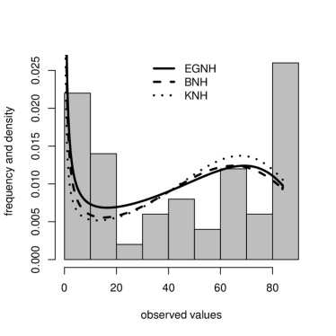
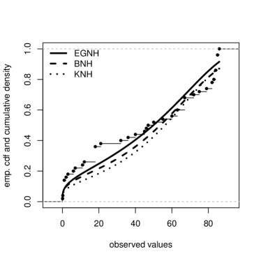
Based on the figures of merit in Table 6, the proposed EGNH distribution presents smallest GoF values. Figure 9(a) displays fitted and empirical densities for this dataset. We consider only EGNH, KNH and BNH models because these models present the smallest values of the KS statistic. The EGNH and KNH distributions seems to provide a closer fit to the histogram. The empirical cdf and the fitted cdfs of these models are displayed in Figure 10(a). From this plot, we note that the EGNH model provides a good fit.

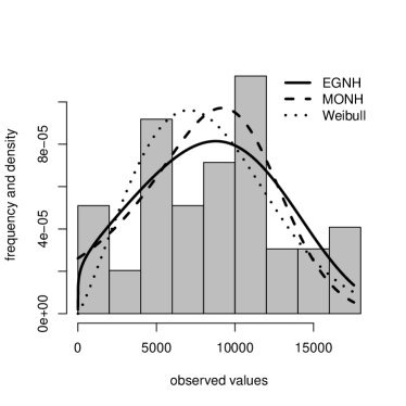
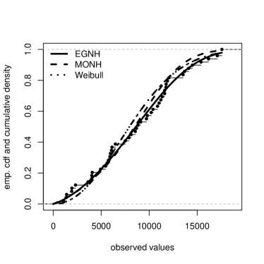
On the other hand, with respect to Table 7, notice that the proposed EGNH model presents smallest values for the W*, A* and KS statistics. The fitted EGNH, MONH and Weibull pdfs in Figure 9(b) reveal that the proposed model fits current data better than others. The use of AIC, BIC, CAIC and HQIC is only recommended to compare nested models, then it is not adequate to compare the Weibull and MONH models with the EGNH using these criteria. In Figure 10(b), we can see that the empirical and fitted cdfs, which confirm that the EGNH model is one of the best candidates to describe the second dataset. In summary, the EGNH model may be an interesting alternative to other models available in the literature for modelling positive real data.

Table 6: Goodness-of-fit tests for Aarset’s dataset
model W* A* KS AIC CAIC BIC HQIC
EGNH(α,β,a,b)EGNH𝛼𝛽𝑎𝑏\operatorname{\mathrm{EGNH}}(\alpha,\beta,a,b) 0.191 1.381 0.141 454.73 455.62 462.38 457.64
BNH(α,β,a,b)𝛼𝛽𝑎𝑏(\alpha,\beta,a,b) 0.198 1.409 0.131 457.56 458.45 465.21 460.47
KNH(α,β,a,b)𝛼𝛽𝑎𝑏(\alpha,\beta,a,b) 0.209 1.479 0.129 459.44 460.34 467.09 462.36
MNH(α,a,b)𝛼𝑎𝑏(\alpha,a,b) 0.286 1.877 0.164 475.73 476.25 481.47 477.92
MONH(α,a,b)𝛼𝑎𝑏(\alpha,a,b) 0.314 2.028 0.160 477.64 478.17 483.38 479.83
TNH(α,a,b)𝛼𝑎𝑏(\alpha,a,b) 0.333 2.132 0.173 477.89 478.42 483.63 480.08
ENH(α,a,b)𝛼𝑎𝑏(\alpha,a,b) 0.349 2.219 0.204 472.36 472.88 478.09 474.55
ZBNH(α,a,b)𝛼𝑎𝑏(\alpha,a,b) 0.359 2.279 0.199 473.61 474.13 479.34 475.79
GPW(a,b,c)𝑎𝑏𝑐(a,b,c) 0.372 2.341 0.194 475.89 476.42 481.63 478.07
NH(a,b)𝑎𝑏(a,b) 0.342 2.181 0.178 476.02 476.27 479.84 477.47
EE(α,β)𝛼𝛽(\alpha,\beta) 0.485 2.950 0.204 483.99 484.25 487.81 485.45
Weibull(a,b)𝑎𝑏(a,b) 0.496 3.008 0.193 486.00 486.26 489.83 487.46
Table 7: Goodness-of-fit tests for Andrews and Herzberg’s dataset
model W* A* KS AIC CAIC BIC HQIC
EGNH(α,β,a,b)𝛼𝛽𝑎𝑏(\alpha,\beta,a,b) 0.032 0.236 0.069 966.81 967.72 974.38 969.68
MONH(α,a,b)𝛼𝑎𝑏(\alpha,a,b) 0.033 0.246 0.072 965.42 965.95 971.09 967.57
BNH(α,β,a,b)𝛼𝛽𝑎𝑏(\alpha,\beta,a,b) 0.033 0.237 0.070 966.95 967.86 974.51 969.82
ZBNH(α,a,b)𝛼𝑎𝑏(\alpha,a,b) 0.054 0.323 0.079 965.49 966.02 971.17 967.64
GPW(a,b,c)𝑎𝑏𝑐(a,b,c) 0.057 0.361 0.191 968.59 969.12 974.26 970.74
ENH(α,a,b)𝛼𝑎𝑏(\alpha,a,b) 0.058 0.383 0.084 966.26 966.80 971.94 968.42
NH(a,b)𝑎𝑏(a,b) 0.059 0.388 0.186 973.48 973.75 977.27 974.92
Weibull(a,b)𝑎𝑏(a,b) 0.073 0.482 0.088 965.70 965.95 969.48 967.13
KNH(α,β,a,b)𝛼𝛽𝑎𝑏(\alpha,\beta,a,b) 0.075 0.496 0.089 969.79 970.70 977.36 972.66
EE(α,β)𝛼𝛽(\alpha,\beta) 0.164 1.061 0.118 972.14 972.40 975.92 973.58
MNH(α,a,b)𝛼𝑎𝑏(\alpha,a,b) 0.342 2.137 0.277 1021.80 1022.34 1027.48 1023.96
Figure 9: Empirical and fitted pdfs
Figure 10: Empirical and fitted pdfs

13 Concluding remarks

In this paper, we propose a new distribution, which is a simple generalization of the Nadarajah-Haghighi’s exponential proposed by Nadarajah and Haghighi (2011). Further, the new model includes others known distributions as special cases. We refer to it as the exponentiated generalized Nararajah-Haghighi (EGNH) distribution. Some of its properties have been derived and discussed: ordinary and incomplete moments, mean deviations, Rényi entropy and order statistics. We present theoretical evidence that the new distribution can take decreasing, increasing, bathtub-shaped and upside-down bathtub hazard rate functions. We provide a maximum likelihood procedure for estimating the EGNH parameters. A Monte Carlo study to assess the consistency of the maximum likelihood estimates is performed, which satisfies the expected asymptotic behavior. The usefulness of the new model is illustrated through two applications to real data. The results indicate that our proposal can furnish better performance than other extended Nadarajah-Haghighi models recorded in the survival literature. The formulae related with the new model are manageable and may turn into adequate tools comprising the arsenal of applied statistics. We hope that the proposed model may attract wider applications for modeling positive real data in many areas such as engineering, survival analysis, hydrology and economics.

References

  • Aarset (1987) Aarset, M. V. 1987. How to Identify a Bathtub Hazard Rate. Reliability, IEEE Transactions on, R-36, 106–108.
  • Abdul Moniem (2015) Abdul Moniem, I. B. 2015. Exponentiated Nadarajah and Haghighi’s exponential Distribution. International Journal of Mathematical Analysis and Applications, 2.
  • Ahmed et al. (2015) Ahmed, A., Muhammed, H. Z., and Elbatal, I. 2015. A New Class of Extension Exponential Distribution. International Journal of Applied Mathematical Sciences, 8, 13–30.
  • Alzaatreh et al. (2013) Alzaatreh, A., Lee, C., and Famoye, F. 2013. A new method for generating families of continuous distributions. METRON - International Journal of statistics, 71, 63–79.
  • Andrade et al. (2015) Andrade, T., Rodrigues, H. M., Bourguignon, M., and Cordeiro, G. M. 2015. The exponentiated generalized Gumbel distribution. Revista Colombiana de Estadística, 38, 123–143.
  • Andrews and Herzberg (1985) Andrews, D. F. and Herzberg, A. M. 1985. Stress-Rupture Life of Kevlar 49/Epoxy Spherical Pressure Vessels, (pp. 181–186). New York, NY: Springer New York.
  • Bourguignon et al. (2015) Bourguignon, M., Lima, M. C. S., Leão, J., Nascimento, A. D. C., Pinho, L. G. B., and Cordeiro, G. M. 2015. A new generalized gamma distribution with applications. American Journal of Mathematical and Management Sciences, 34, 309–342.
  • Bourguignon et al. (2014) Bourguignon, M., Silva, R. B., and Cordeiro, G. M. 2014. The Weibull-G Family of Probability Distributions. Journal of Data Science, 12, 53–68.
  • Cooray and Ananda (2008) Cooray, K. and Ananda, M. M. A. 2008. A Generalization of the Half-Normal Distribution with Applications to Lifetime Data. Communications in Statistics - Theory and Methods, 37, 1323–1337.
  • Cordeiro and Castro (2011) Cordeiro, G. M. and Castro, M. 2011. A new family of generalized distributions. Journal of Statistical Computation and Simulation, 81, 883–898.
  • Cordeiro et al. (2013) Cordeiro, G. M., Ortega, E. M. M., and Cunha, D. C. C. 2013. The Exponentiated Generalized Class of Distributions. Journal of Data Science, 1, 1–27.
  • Cordeiro et al. (2011) Cordeiro, G. M., Ortega, E. M. M., and Silva, G. O. 2011. The exponentiated generalized gamma distribution with application to lifetime data. Journal of Statistical Computation and Simulation, 81, 827–842.
  • Dias (2016) Dias, C. R. B. 2016. New Continuous Distributions Applied To Lifetime Data And Survival Analysis. Doctoral thesis, Universidade Federal de Pernambuco, Recife.
  • El Damcese and Ramadan (2015) El Damcese, M. A. and Ramadan, D. A. 2015. Studies on Properties and Estimation Problems for Modified Extension of Exponential Distribution. International Journal of Computer Applications, 125.
  • Elbatal and Muhammed (2014) Elbatal, I. and Muhammed, H. Z. 2014. Exponentiated Generalized Inverse Weibull Distribution. Applied Mathematical Sciences, 8, 3997–4012.
  • Eugene et al. (2002) Eugene, N., Lee, C., and Famoye, F. 2002. Beta-normal Distribution And Its Applications. Communications in Statistics - Theory and Methods, 31, 497–512.
  • Gupta et al. (1998) Gupta, R. C., Gupta, P. L., and Gupta, R. D. 1998. Modeling failure time data by lehman alternatives. Communications in Statistics - Theory and Methods, 27, 887–904.
  • Gupta and Kundu (2001) Gupta, R. D. and Kundu, D. 2001. Exponentiated Exponential Family. Biometrical Journal, 43, 117–130.
  • Henningsen and Toomet (2011) Henningsen, A. and Toomet, O. 2011. maxLik: A package for maximum likelihood estimation in R. Computational Statistics, 26, 443–458.
  • Kenney and Keeping (1962) Kenney, J. F. and Keeping, E. S. 1962. Mathematics of statistics (3 ed.)., volume 1. Van Nostrand, New Jersey: Chapman & Hall Ltd.
  • Lee et al. (2013) Lee, C., Famoye, F., and Alzaatreh, A. Y. 2013. Methods for generating families of univariate continuous distributions in the recent decades. Wiley Interdisciplinary Reviews, 5, 219–238.
  • Lemonte (2013) Lemonte, A. J. 2013. A new exponential-type distribution with constant, decreasing, increasing, upside-down bathtub and bathtub-shaped failure rate function. Computational Statistics & Data Analysis, 62, 149–170.
  • Lemonte and Cordeiro (2011) Lemonte, A. J. and Cordeiro, G. M. 2011. The exponentiated generalized inverse Gaussian distribution. Statistics & Probability Letters, 81, 506–517.
  • Lemonte et al. (2016) Lemonte, A. J., Cordeiro, G. M., and Moreno Arenas, G. 2016. A new useful three-parameter extension of the exponential distribution. Statistics, 50, 312–337.
  • Lima (2015) Lima, S. R. L. 2015. The Half-Normal Generalized Family And Kumaraswamy Nadarajah-Haghighi Distribution. Master thesis, Universidade Federal de Pernambuco.
  • Moors (1988) Moors, J. J. A. 1988. A Quantile Alternative for Kurtosis. Journal of the Royal Statistical Society. Series D (The Statistician), 37, 25–32.
  • Mudholkar and Srivastava (1993) Mudholkar, G. S. and Srivastava, D. K. 1993. Exponentiated Weibull family for analyzing bathtub failure-rate data. Reliability, IEEE Transactions on, 42, 299–302.
  • Mudholkar et al. (1995) Mudholkar, G. S., Srivastava, D. K., and Freimer, M. 1995. The Exponentiated Weibull Family: A Reanalysis of the Bus-Motor-Failure Data. Technometrics, 37, 436–445.
  • Nadarajah and Gupta (2007) Nadarajah, S. and Gupta, A. K. 2007. A product Pareto distribution. Metrika, 68, 199–208.
  • Nadarajah and Haghighi (2011) Nadarajah, S. and Haghighi, F. 2011. An extension of the exponential distribution. Statistics, 45, 543–558.
  • Nikulin and Haghighi (2006) Nikulin, M. and Haghighi, F. 2006. A Chi-Squared Test for the Generalized Power Weibull Family for the Head-and-Neck Cancer Censored Data. Journal of Mathematical Sciences, 133, 1333–1341.
  • Nikulin and Haghighi (2009) Nikulin, M. and Haghighi, F. 2009. On the power generalized Weibull family. METRON - International Journal of statistics, LXVII, 75–86.
  • Ortega et al. (2015) Ortega, E. M. M., Lemonte, A. J., Silva, G. O., and Cordeiro, G. M. 2015. New flexible models generated by gamma random variables for lifetime modeling. Journal of Applied Statistics, 42, 2159–2179.
  • Selim and Badr (2016) Selim, M. A. and Badr, A. M. 2016. The Kumaraswamy Generalized Power Weibull Distribution. Mathematical Theory and Modeling, 6, 110–124.
  • Silva et al. (2015) Silva, R. V., Gomes Silva, F., Ramos, M. W. A., and Cordeiro, G. M. 2015. A New Extended Gamma Generalized Model. International Journal of Pure and Applied Mathematics, 100.
  • Zografos and Balakrishnan (2009) Zografos, K. and Balakrishnan, N. 2009. On families of beta- and generalized gamma-generated distributions and associated inference. Statistical Methodology, 6, 344–362.