Hit-and-Run for Sampling and Planning in Non-Convex Spaces

Abstract

We propose the Hit-and-Run algorithm for planning and sampling problems in non-convex spaces. For sampling, we show the first analysis of the Hit-and-Run algorithm in non-convex spaces and show that it mixes fast as long as certain smoothness conditions are satisfied. In particular, our analysis reveals an intriguing connection between fast mixing and the existence of smooth measure-preserving mappings from a convex space to the non-convex space. For planning, we show advantages of Hit-and-Run compared to state-of-the-art planning methods such as Rapidly-Exploring Random Trees.

1 Introduction

Rapidly-Exploring Random Trees (RRT) (LaValle, 1998, LaValle and Kuffner Jr., 2001) is one of the most popular planning algorithms, especially when the search space is high-dimensional and finding the optimal path is computationally expensive. RRT performs well on many problems where classical dynamic programming based algorithms, such as A*, perform poorly. RRT is essentially an exploration algorithm, and in the most basic implementation, the algorithm even ignores the goal information, which seems to be a major reason for its success. Planning problems, especially those in robotics, often feature narrow pathways connecting large explorable regions; combined with high dimensionality, this means that finding the optimal path is usually intractable. However, RRT often provides a feasible path quickly.

Although many attempts have been made to improve the basic algorithm (Abbasi-Yadkori et al., 2010, Karaman and Frazzoli, 2010, 2011), RRT has proven difficult to improve upon. In fact, given extra computation, repeatedly running RRT often produces competitive solutions. In this paper, we show that a simple alternative greatly improves upon RRT. We propose using the Hit-and-Run algorithm for feasible path search. Arguably simpler than RRT, the Hit-and-Run is a rapidly mixing MCMC sampling algorithm for producing a point uniformly at random from a convex space (Smith, 1984). color=blue!20!white,]Victor: not that clear, you mean hnr is simpler that RRT? insist maybe more on what still need to be improved from RRT or say that you will detail later Not only Hit-and-Run finds a feasible path faster than RRT, it is also more robust with respect to the geometry of the space.

Before giving more details, we define the planning and sampling problems that we consider. Let $\Sigma$ be a bounded connected subset of $\mathbb{R}^{n}$. For points $a,b\in\Sigma$, we use $[a,b]$ to denote their (one-dimensional) convex hull. Given a starting point $a_{1}$ and a goal region ${\cal G}\subset\Sigma$, the planning problem is to find a sequence of points $\{a_{1},a_{2},\dots,a_{\tau}\}$ for $\tau\geq 1$ such that all points are in $\Sigma$, $a_{\tau}$ is in ${\cal G}$, and for $t=2,\dots,\tau$, $[a_{t-1},a_{t}]\subset\Sigma$.

The sampling problem is to generate points uniformly at random from $\Sigma$. Sampling is often difficult, but Markov Chain Monte Carlo (MCMC) algorithms have seen empirical and theoretical success (Lovász and Vempala, 2007). MCMC algorithms, such as Hit-and-Run and Ball-Walk (Vempala, 2005), sample a Markov Chain on $\Sigma$ that has a stationary distribution equal to the uniform distribution on $\Sigma$; then, if we run the Markov Chain long enough, the marginal distribution of the sample is guaranteed to come from a distribution exponentially close to the target distribution. Solving the sampling problem yields a solution to the planning problem; one can generate samples and terminate when $a_{t}$ hits ${\cal G}$.

Figure 1: RRT (left) and Hit-and-Run (right)

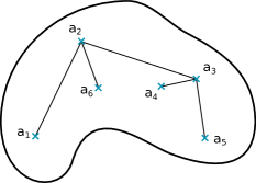
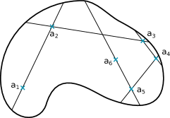
Let us define Hit-and-Run and the RRT algorithms (see also Figure 1 for an illustration). Hit-and-Run defines a Markov chain on $\Sigma$ where the transition dynamics are as follows. A direction is chosen uniformly at random, and $a_{t+1}$ is chosen uniformly from the largest chord contained in $\Sigma$ in this direction passing through $a_{t}$. This Markov Chain has a uniform stationary distribution on $\Sigma$ (Smith, 1984). As a planning algorithm, this chain continues until it hits the goal region. Let $\tau$ be the stopping time. The solution path is $\{a_{1},a_{2},\dots,a_{\tau}\}$.

On the other hand, the RRT algorithm iteratively builds a tree $T$ with $a_{1}$ as a root and nodes labeled as $a^{n}\in\Sigma$ and edges $\{a^{m},a^{n}\}$ that satisfy $[a^{m},a^{n}]\subseteq\Sigma$. To add a point to the tree, $a^{r}$ is uniformly sampled from $\Sigma$ and its nearest neighbor $a^{n}\in T$ is computed. If $[a^{n},a^{r}]\subset\Sigma$, then node $a^{r}$ and edge $[a^{n},a^{r}]$ are added to $T$. Otherwise, we search for the point $a^{e}\in[a^{n},a^{r}]$ farthest from $a^{n}$ such that $[a^{n},a^{e}]\subseteq\Sigma$. Then $a^{e}$ and $[a^{n},a^{e}]$ are added to the tree. This process is continued until we add an edge terminating in ${\cal G}$ and the sequence of points on that branch is returned as the solution path. In the presence of dynamic constraints, a different version of RRT that makes only small local steps is used. These versions will be discussed in the experiments section.

There are two main contributions on this paper. First, we analyze the Hit-and-Run algorithm in a non-convex space and show that the mixing time is polynomial in dimensionality as long as certain smoothness conditions are satisfied. The mixing time of Hit-and-Run for convex spaces is known to be polynomial (Lovász, 1999). However, to accommodate planning problems, we focus on non-convex spaces. Our analysis reveals an intriguing connection between fast mixing and the existence of smooth measure-preserving mappings. The only existing analysis of random walk algorithms in non-convex spaces is due to Chandrasekaran et al. (2010) who analyzed Ball-Walk in star-shaped bodies. Second, we propose Hit-and-Run for planning problems as an alternative to RRT and show that it finds a feasible path quickly. From the mixing rate, we obtain a bound on the expected length of the solution path in the planning problem. Such performance guarantees are not available for RRT.

The current proof techniques in the analysis of Hit-and-Run heavily rely on the convexity of the space. It turns out that non-convexity is specially troubling when points are close to the boundary. We overcome these difficulties as follows. First, Lovász and Vempala (2006) show a tight isoperimetic inequality in terms of average distances instead of minimum distances. This enables us to ignore points that are sufficiently close to the boundary. Next we show that as long as points are sufficiently far from the boundary, the cross-ratio distances in the convex and non-convex spaces are closely related. Finally we show that, given a curvature assumption, if two points are close geometrically and are sufficiently far from the boundary, then their proposal distributions must be close as well. color=blue!20!white,]Victor: what is a proposal distribution? color=blue!20!white,]Victor: theoretical results for RRT in the litterature?

Hit-and-Run has a number of advantages compared to RRT; it does not require random points sampled from the space (which is itself a hard problem), and it is guaranteed to reach the goal region with high probability in a polynomial number of rounds. In contrast, there are cases where RRT growth can be very slow (see the experiments sections for a discussion). Moreover, Hit-and-Run provides safer solutions, as its paths are more likely to stay away from the boundary. In contrast, a common issue with RRT solutions is that they tend to be close to the boundary. Because of this, further post-processing steps are needed to smooth the path.

color=blue!20!white,]Victor: insist more on the fact that you do not change hitand run or propose a new version just show that the original algo is the solution and you provide the analysis which is cool

1.1 Notation

For a set $K$, we will denote the $n$-dimensional volume by $\textsc{vol}(K)$, the $(n-1)$-dimensional surface volume by $S_{K}=\textsc{vol}_{n-1}(\partial K)$, and the boundary by $\partial K$. The diameter of $K$ is $D_{K}=\max_{x,x^{\prime}\in K}\left|x-x^{\prime}\right|$, where $\left|\cdot\right|$ will be used for absolute value and Euclidean norm, and the distance between sets $K_{1}$ and $K_{2}$ is defined as $d(K_{1},K_{2})=\min_{x\in K_{1},y\in K_{2}}\left|x-y\right|$. Similarly, $d(x,K)=d(\{x\},K)$. For a set $K$, we use $K^{\epsilon}$ to denote $\{x\in K\,:\,d(x,\partial K)\geq\epsilon\}$. Finally, for distributions $P$ and $Q$, we use $d_{tv}(P,Q)$ to denote the total variation distance between $P$ and $Q$.

We will also need some geometric quantities. We will denote lines (i.e., 1-dimensional affine spaces) by $\ell$. For $x,y\in K$, we denote their convex hull, that is, the line segment between them, by $[x,y]$ and $\ell(x,y)$ the line that passes through $x$ and $y$ (which contains $[x,y]$). We also write $[x_{1},\ldots,x_{k}]$ to denote that $x_{1},\ldots,x_{k}$ are collinear.

We also use $\ell_{K}(x,y)$ to denote the longest connected chord through $x\in K$ and $y\in K$ contained in $K$ and $|\ell_{K}(x,y)|$ its length. We use $a(x,y)$ and $b(x,y)$ to denote the endpoints of $\ell_{K}(x,y)$ that are closer to $x$ and $y$, respectively, so that $\ell_{K}(x,y)=[a(x,y),b(x,y)]=[b(y,x),a(y,x)]$. The Euclidean ball of unit radius centered at the origin, $B_{n}(0,1)\subset\mathbb{R}^{n}$, has volume $\pi_{n}$. We use $x_{1:m}$ to denote the sequence $x_{1},\dots,x_{m}$. Finally we use $a\wedge b$ to denote $\min(a,b)$.

2 Sampling from Non-Convex Spaces

Most of the known results for the sampling times of the Hit-and-Run exist for convex sets only. We will think of $\Sigma$ as the image of some convex set $\Omega$ under a measure preserving, bilipschitz function $g$. The goal is to understand the relevant geometric quantities of $\Sigma$ through properties of $g$ and geometric properties of $\Omega$. We emphasize that the existence of the map $g$ and its properties are necessary for the analysis, but the actual algorithm does not need to know $g$. We formalize this assumption below as well as describe how we interact with $\Sigma$ and present a few more technical assumptions required for our analysis. We then present our main result, and follow that with some conductance results before moving on to the proof of the theorem in the next section.

Assumption 1 (Oracle Access).

Given a point $u$ and a line $\ell$ that passes through $u$, the oracle returns whether $u\in\Sigma$, and, if so, the largest connected interval in $\ell\cap\Sigma$ containing $u$.

Assumption 2 (Bilipschitz Measure-Preserving Embeddings).

There exist a convex set $\Omega\subset\mathbb{R}^{n}$ and a bilipschitz, measure-preserving map $g$ such that $\Sigma$ is the image of $\Omega$ under $g$. That is, there exists a function $g$ with $\left|D_{g}(x)\right|=1$ (i.e. the Jacobian has unit determinant) with constants $L_{\Sigma}$ and $L_{\Omega}$ such that, for any $x,y\in\Omega$,

$$\frac{1}{L_{\Omega}}\left|x-y\right|\leq\left|g(x)-g(y)\right|\leq L_{\Sigma}\left|x-y\right|.$$

In words, $g$ is measure-preserving, $g$ is $L_{\Sigma}$-Lipschitz, and $g^{-1}$ is $L_{\Omega}$-Lipschitz.

As an example, Fonseca and Parry (1992) shows that for any star-shaped space, a smooth measure-preserving embedding exists. One interesting consequence of Assumption 2 is that because the mapping is measure-preserving, there must exist a pair $x,y\in\Omega$ such that $\left|g(x)-g(y)\right|\geq\left|x-y\right|$. Otherwise, $\int_{\Omega}g\leq 1$, a contradiction. Similarly, there must exist a pair $u,v\in\Sigma$ such that $\left|g^{-1}(u)-g^{-1}(v)\right|\geq\left|u-v\right|$. Thus,

$$L_{\Omega},L_{\Sigma}\geq 1\;.$$ (1)

To simplify the analysis, we will assume that $\Omega$ is a ball with radius $r$. In what follows, we use $x,y,z$ to denote points in $\Omega$, and $u,v,w$ to denote points in $\Sigma$. We will also assume that $\Sigma$ has no sharp corners and has a smooth boundary:

Assumption 3 (Low Curvature).

For any two dimensional plane ${\cal H}\subset\mathbb{R}^{n}$, let $\kappa_{\cal H}$ be the curvature of $\partial\Sigma\cap{\cal H}$ and ${\cal R}_{\cal H}$ be the perimeter of $\partial\Sigma\cap{\cal H}$. We assume that $\Sigma$ has low curvature, i.e. that $\kappa=\sup_{\cal H}\kappa_{\cal H}{\cal R}_{\cal H}$ is finite.

Assumption 2 does not imply low curvature, as there exist smooth measure-preserving mappings from the unit ball to a cube (Griepentrog et al., 2008).

Assumption 4.

We assume that the volume of $\Sigma$ is equal to one. We also assume that $\Sigma$ contains a Euclidean ball of radius one.

Note that the unit ball has volume less than 1 for $n>12$, so for small dimensional problems, we will need to relax this assumption.

We motivate the forthcoming technical machinery by demonstrating what it can accomplish. The following theorem is the main result of the paper, and the proof makes up most of Section 3.

Theorem 5.

Consider the Hit-and-Run algorithm. Let $\sigma_{0}$ be the distribution of the initial point given to Hit-and-Run, $\sigma_{t}$ be the distribution after $t$ steps of Hit-and-Run, and $\sigma$ be the stationary distribution (which is uniform). Let $M=\sup_{A}\sigma_{0}(A)/\sigma(A)$. Let $\epsilon$ be a positive scalar. After

$$t\geq C^{\prime}n^{6}\log\frac{M}{\epsilon}$$

steps, we have $d_{tv}(\sigma_{t},\sigma)\leq\epsilon$. Here $C^{\prime}$ is a low order polynomial of $L_{\Omega},L_{\Sigma},\kappa$.

3 Analysis

This section proves Theorem 5. We begin by stating a number of useful geometrical results, which allow us to prove the two main components: an isoperimetric inequality in Section 3.2 and a total variation inequality in Section 3.3. We then combine everything in Section 3.4.

3.1 Fast Mixing Markov Chains

We rely on the notion of conductance color=blue!20!white,]Victor: reference? as our main technical tool. This section recalls the relevant results.

We say that points $u,v\in\Sigma$ see each other if $[u,v]\subseteq\Sigma$. We use $\textsc{view}(u)$ to denote all points in $\Sigma$ visible from $u$. Let $\ell_{\Sigma}(u,v)$ denote the chord through $u$ and $v$ inside $\Sigma$ and $\left|\ell_{\Sigma}(u,v)\right|$ its length. Let $P_{u}(A)$ be the probability of being in set $A\subset\Sigma$ after one step of Hit-and-Run from $u$ and $f_{u}$ its density function. By an argument similar to the argument in Lemma 3 of Lovász (1999), we can show that

$$f_{u}(v)=2\frac{\mathbf{1}\left\{v\in\textsc{view}(u)\right\}}{n\pi_{n}\left|\ell_{\Sigma}(u,v)\right|\cdot\left|u-v\right|^{n-1}}\;.$$ (2)

The conductance of the Markov process is defined as

$$\Phi=\inf_{A\subset\Sigma}\frac{\int_{A}P_{u}(\Sigma\setminus A)du}{\min(\textsc{vol}(A),\textsc{vol}(\Sigma\setminus A))}\;.$$

We begin with a useful conductance result that applies to general Markov Chains.

Lemma 6 (Corollary 1.5 of Lovász and Simonovits (1993)).

Let $M=\sup_{A}\sigma_{0}(A)/\sigma(A)$. Then for every $A\subset\Sigma$,

$$\left|\sigma_{t}(A)-\sigma(A)\right|\leq\sqrt{M}\left(1-\frac{\Phi^{2}}{2}\right)^{t}\;.$$

Proving a lower bound on the conductance is therefore a key step in the mixing time analysis. Previous literature has shown such lower bounds for convex spaces. Our objective in the following is to obtain such bounds for more general non-convex spaces that satisfy bilipschtiz measure-preserving embedding and low curvature assumptions. color=blue!20!white,]Alan: Maybe Add a comment about how this part of the paper applies for general Markov chains even though they are studying random walks on a convex body.

As in previous literature, we shall find that the following cross-ratio distance is very useful in deriving an isoperimetric inequality and a total variation inequality.

Definition 1.

Let $[a,u,v,b]$ be collinear and inside $\Sigma$, such that $a,b\in\partial\Sigma$. Define

$$d_{\Sigma}(u,v)=\frac{\left|a-b\right|\left|u-v\right|}{\left|a-u\right|\left|v-b\right|}\;.$$

It is easy to see that $d_{\Sigma}(u,v)\geq 4\left|u-v\right|/D_{\Sigma}$. We define the following distance measure for non-convex spaces.

Definition 2.

A set $\Sigma$ will be called $\tau$-best if, for any $u,v\in\Sigma$, there exist points $z_{1},\ldots,z_{\tau-1}$ such that $[u,z_{1}],[z_{\tau-1},v]$, and $[z_{i},z_{i+1}]$ for $i=1,\ldots,\tau-2$ are all in $\Sigma$; i.e., any two points in $\Sigma$ can be connected by $\tau$ line segments that are all inside $\Sigma$. We define the distance

$$\widetilde{d}_{\Sigma}(u,v) =\inf_{z_{1:\tau-1}\in\Sigma}\big{(}d_{\Sigma}(u,z_{1})+d_{\Sigma}(z_{1},z_{2})+\dots+d_{\Sigma}(z_{\tau-1},v)\big{)}\;,$$

and, by extension, the distance between two subsets $\Sigma_{1},\Sigma_{2}\subset\Sigma$ as $\widetilde{d}_{\Sigma}(\Sigma_{1},\Sigma_{2})=\inf_{u\in\Sigma_{1},v\in\Sigma_{2}}\widetilde{d}_{\Sigma}(u,v)$.

The analysis of the conductance is often derived via an isoperimetric inequality.

Theorem 7 (Theorem 4.5 of Vempala (2005)).

Let $\Omega$ be a convex body in $\mathbb{R}^{n}$. Let $h:\Omega\rightarrow\mathbb{R}^{+}$ be an arbitrary function. Let $(\Omega_{1},\Omega_{2},\Omega_{3})$ be any partition of $\Omega$ into measurable sets. Suppose that for any pair of points $x\in\Omega_{1}$ and $y\in\Omega_{2}$ and any point $z$ on the chord of $\Omega$ through $x$ and $y$, $h(z)\leq(1/3)\min(1,d_{\Omega}(x,y))$. Then

$$\textsc{vol}(\Omega_{3})\geq\mathbf{E}_{\Omega}(h)\min(\textsc{vol}(\Omega_{1}),\textsc{vol}(\Omega_{2}))\,,$$

where the expectation is defined with respect to the uniform distribution on $\Omega$.

Given an isoperimetric inequality, a total variation inequality is typically used in a mixing time analysis to lower bound cross-ratio distances and then lower bound the conductance. Our approach is similar. We use the embedding assumption to derive an isoperimetric inequality in the non-convex space $\Sigma$. Then we relate cross-ratio distance $d_{\Omega}$ to distance $\widetilde{d}_{\Sigma}$. This approximation is good when the points are sufficiently far from the boundary. We incur a small error in the mixing bound by ignoring points that are too close to the boundary. Finally we use the curvature condition to derive a total variation inequality and to lower bound the conductance.

3.2 Cross-Ratio Distances

The first step is to show the relationship between cross-ratio distances in the convex and non-convex spaces. We show that these distances are close as long as points are far from the boundary. These results will be used in the proof of the main theorem in Section 3.4 to obtain an isoperimetric inequality in the non-convex space. First we define a useful quantity.

Definition 3.

Consider a convex set $\Omega$ with some subset $\Omega^{\prime}$ and collinear points $\{a,x,b\}$ with $a,b\in\partial\Omega$, $x\in\Omega^{\prime}$, and $\left|x-b\right|\leq\left|x-a\right|$. Let $c$ be a point on $\partial\Omega$. Let $R(a,x,b,c)=\left|x-b\right|/\left|x-c\right|$. We use $R(\Omega,\Omega^{\prime})$ to denote the maximum of $R(a,x,b,c)$ over all such points. We use $R_{\epsilon}$ to denote $R(\Omega,\Omega^{\epsilon})$.

The following lemma is the main technical lemma, and we use it to express $\widetilde{d}_{\Sigma}$ in terms of $d_{\Omega}$.

Lemma 8.

Let $\epsilon$ be a positive scalar such that $R_{\epsilon}(1+8R_{\epsilon})\geq 2/3$. Let $\{a,x_{1},x_{2},b\}$ be collinear such that $a$ and $b$ are on the boundary of $\Omega$, $x_{1},x_{2}\in\Omega^{\epsilon}$, and $\left|x_{1}-a\right|<\left|x_{2}-a\right|$. Let $c$ and $d$ be two points on the boundary of $\Omega$. Then

$$\frac{\left|b-a\right|}{\left|a-x_{1}\right|}\cdot\frac{\left|x_{1}-c\right|}{\left|c-d\right|}\cdot\frac{\left|d-x_{2}\right|}{\left|x_{2}-b\right|}\geq\frac{1}{4R_{\epsilon}(1+2R_{\epsilon})}\;.$$

Proof.

Let

$$A=\frac{\left|b-a\right|\left|x_{1}-x_{2}\right|}{\left|a-x_{1}\right|\left|x_{2}-b\right|}\,,\qquad B=\frac{\left|c-d\right|\left|x_{1}-x_{2}\right|}{\left|c-x_{1}\right|\left|x_{2}-d\right|}\;.$$

We prove the claim by proving that $A/B\geq 1/(4R_{\epsilon}(1+2R_{\epsilon}))$.
Case 1, $\left|x_{1}-b\right|\leq\left|x_{1}-a\right|$: In this case, $x_{1}$ and $x_{2}$ are both on the line segment $[(a+b)/2,b]$. We consider two cases.
Case 1.1, $\left|x_{2}-d\right|\leq\left|x_{2}-b\right|$: We have that

$$\left|c-d\right|=\left|c-x_{1}\right|+\left|x_{1}-x_{2}\right|+\left|x_{2}-d\right|\leq\left|c-x_{1}\right|+\left|x_{1}-b\right|+\left|x_{2}-b\right|\;.$$ (3)

Because $\left|x_{1}-a\right|<\left|x_{2}-a\right|$ by the assumption of the lemma, we have $\left|x_{2}-b\right|<\left|x_{1}-b\right|$. Also because $\left|x_{1}-b\right|\leq\left|x_{1}-a\right|$ in Case 1, we have $\left|x_{1}-b\right|/\left|c-x_{1}\right|\leq R_{\epsilon}$. Thus

$$\frac{\left|x_{2}-b\right|}{\left|c-x_{1}\right|}\leq\frac{\left|x_{1}-b\right|}{\left|c-x_{1}\right|}\leq R_{\epsilon}\;.$$ (4)

By (3) and (4),

$$\frac{\left|c-d\right|}{\left|c-x_{1}\right|}\leq 1+\frac{\left|x_{1}-b\right|}{\left|c-x_{1}\right|}+\frac{\left|x_{2}-b\right|}{\left|c-x_{1}\right|}\leq 1+R_{\epsilon}+\frac{\left|x_{2}-b\right|}{\left|c-x_{1}\right|}\leq 1+2R_{\epsilon}\;.$$

We use also that by definition of $R_{\epsilon}$ $\left|x_{2}-b\right|\leq R_{\epsilon}\left|x_{2}-d\right|$. This and the previous result lets us bound

$$B \leq(1+2R_{\epsilon})\frac{\left|x_{1}-x_{2}\right|}{\left|x_{2}-d\right|}\,,$$

$$A \geq\frac{\left|b-a\right|\left|x_{1}-x_{2}\right|}{R_{\epsilon}\left|a-x_{1}\right|\left|x_{2}-d\right|}\geq\frac{\left|x_{1}-x_{2}\right|}{R_{\epsilon}\left|x_{2}-d\right|}\,,$$

and conclude

$$\frac{A}{B}\geq\frac{1}{R_{\epsilon}(1+2R_{\epsilon})}\geq\frac{1}{4R_{\epsilon}(1+2R_{\epsilon})}\;.$$

Case 1.2, $\left|x_{2}-d\right|>\left|x_{2}-b\right|$:
Case 1.2.1, $\left|c-x_{1}\right|\leq\left|x_{2}-d\right|$: We have that $\left|x_{2}-b\right|<\left|x_{1}-b\right|\leq R_{\epsilon}\left|x_{1}-c\right|$. Thus,

$$\frac{A}{B} \geq\frac{\left|a-b\right|\left|x_{1}-x_{2}\right|}{BR_{\epsilon}\left|a-x_{1}\right|\left|x_{1}-c\right|}$$

$$=\frac{\left|a-b\right|}{R_{\epsilon}\left|a-x_{1}\right|}\cdot\frac{\left|d-x_{2}\right|}{\left|c-d\right|}\geq\frac{\left|d-x_{2}\right|}{R_{\epsilon}\left|c-d\right|}$$

$$\geq\frac{\left|d-x_{2}\right|}{R_{\epsilon}(\left|d-x_{2}\right|+\left|x_{2}-x_{1}\right|+\left|x_{1}-c\right|)}$$

$$\geq\frac{\left|d-x_{2}\right|}{R_{\epsilon}(\left|d-x_{2}\right|+(1+R_{\epsilon})\left|x_{1}-c\right|)}$$

$$=\frac{1}{R_{\epsilon}\left(1+(1+R_{\epsilon})\frac{\left|x_{1}-c\right|}{\left|d-x_{2}\right|}\right)}\geq\frac{1}{R_{\epsilon}(2+R_{\epsilon})}$$

$$\geq\frac{1}{4R_{\epsilon}(1+2R_{\epsilon})}\;.$$

Case 1.2.2, $\left|c-x_{1}\right|>\left|x_{2}-d\right|$: As before, we bound $A$ and $B$ separately:

$$B \leq\frac{\left|c-d\right|\left|x_{1}-x_{2}\right|}{\left|c-x_{1}\right|\left|x_{2}-b\right|}$$

$$\leq\frac{\left|x_{1}-x_{2}\right|}{\left|x_{2}-b\right|}\cdot\frac{\left|c-x_{1}\right|+R_{\epsilon}\left|c-x_{1}\right|+\left|x_{2}-d\right|}{\left|c-x_{1}\right|}$$

$$\leq(2+R_{\epsilon})\frac{\left|x_{1}-x_{2}\right|}{\left|x_{2}-b\right|}\,,$$

and

$$A=\frac{\left|b-a\right|\left|x_{1}-x_{2}\right|}{\left|a-x_{1}\right|\left|x_{2}-b\right|}\geq\frac{\left|x_{1}-x_{2}\right|}{\left|x_{2}-b\right|}\;.$$

Putting these together,

$$\frac{A}{B}\geq\frac{1}{2+R_{\epsilon}}\geq\frac{1}{4R_{\epsilon}(1+2R_{\epsilon})}\,,$$

where the second inequality holds because $R_{\epsilon}(1+8R_{\epsilon})\geq 2/3$.
Case 2, $\left|x_{1}-b\right|>\left|x_{1}-a\right|$ and $\left|x_{2}-b\right|<\left|x_{2}-a\right|$: In this case, $x_{1}$ and $x_{2}$ are on opposite sides of the point $(a+b)/2$. Let $M$ be a positive constant. We will choose $M=4$ later.
Case 2.1, $\left|c-d\right|\leq M\left|c-x_{1}\right|$: We bound

$$B\leq\frac{M\left|x_{1}-x_{2}\right|}{\left|x_{2}-d\right|}\leq\frac{MR_{\epsilon}\left|x_{1}-x_{2}\right|}{\left|x_{2}-b\right|}$$

and conclude

$$\frac{A}{B}\geq\frac{\left|a-b\right|}{MR_{\epsilon}\left|a-x_{1}\right|}\geq\frac{1}{MR_{\epsilon}}\geq\frac{1}{4R_{\epsilon}(1+2R_{\epsilon})}\;.$$

Case 2.2, $\left|c-d\right|>M\left|c-x_{1}\right|$:
Case 2.2.1, $\left|c-d\right|\leq M\left|a-b\right|$: We have that

$$\frac{A}{B}\geq\frac{1}{MR_{\epsilon}^{2}}\geq\frac{1}{4R_{\epsilon}(1+2R_{\epsilon})}\;.$$

Case 2.2.2, $\left|c-d\right|>M\left|a-b\right|$: Let $x_{0}$ be a point on the line segment $[x_{1},x_{2}]$. Let $\beta_{1}$ be the angle between line segments $[c,x_{1}]$ and $[x_{1},x_{0}]$. We write

$$\left|c-x_{0}\right|^{2} =\left|x_{1}-x_{0}\right|^{2}+\left|x_{1}-c\right|^{2}$$

$$\qquad-2\left|x_{1}-c\right|\cdot\left|x_{1}-x_{0}\right|\cos\beta_{1}$$

$$\leq\frac{1}{M^{2}}\left|c-d\right|^{2}+\frac{1}{M^{2}}\left|c-d\right|^{2}+\frac{2}{M^{2}}\left|c-d\right|^{2}$$

$$=\frac{4}{M^{2}}\left|c-d\right|^{2}\;.$$

By the triangle inequality,

$$\left|d-x_{0}\right|\geq\left|c-d\right|-\left|c-x_{0}\right|\geq\left(1-\frac{2}{M}\right)\left|c-d\right|\;.$$

Let $\beta_{2}$ be the angle between line segments $[d,x_{2}]$ and $[x_{2},x_{0}]$. Let $w=1-2/M$. We write

$$w^{2}\left|c-d\right|^{2} \leq\left|d-x_{0}\right|^{2}$$

$$=\left|x_{2}-x_{0}\right|^{2}+\left|x_{2}-d\right|^{2}-2\left|x_{2}-d\right|\cdot\left|x_{2}-x_{0}\right|\cos\beta_{2}$$

$$\leq\frac{1}{M^{2}}\left|c-d\right|^{2}+\left|x_{2}-d\right|^{2}+\frac{2}{M}\left|d-x_{2}\right|\cdot\left|c-d\right|\;.$$

Thus,

$$\left|x_{2}-d\right|^{2}+\frac{2}{M}\left|d-x_{2}\right|\cdot\left|c-d\right|+\left(\frac{4}{M}-\frac{3}{M^{2}}-1\right)\left|c-d\right|^{2}\geq 0\,,$$

which is a quadratic inequality in $\left|x_{2}-d\right|$. Thus it holds that

$$\left|x_{2}-d\right|\geq\left(-\frac{1}{M}+\left|\frac{2}{M}-1\right|\right)\left|c-d\right|\;.$$

If we choose $M=4$, then $\left|x_{2}-d\right|\geq 0.25\left|c-d\right|$ and

$$B\leq\frac{4\left|x_{1}-x_{2}\right|}{\left|x_{1}-c\right|}\leq\frac{4R_{\epsilon}\left|x_{1}-x_{2}\right|}{\left|x_{1}-a\right|}\;,$$

yielding

$$\frac{A}{B}\geq\frac{\left|a-b\right|}{4R_{\epsilon}\left|b-x_{2}\right|}\geq\frac{1}{4R_{\epsilon}}\geq\frac{1}{4R_{\epsilon}(1+2R_{\epsilon})}\;.$$

Finally, observe that Case 3 follows by symmetry from Case 1. ∎

The following lemma states that the distance $d_{\Omega}$ does not increase by adding more steps.

Lemma 9.

Let $a,y_{1},y_{2},\dots,y_{m},b$ be in the convex body $\Omega$ such that the points $\{a,y_{1},y_{2},\dots,y_{m},b\}$ are collinear. Further assume that $a,b\in\partial\Omega$. We have that

$$d_{\Omega}(y_{1},y_{2})+\dots+d_{\Omega}(y_{m-1},y_{m})\leq d_{\Omega}(y_{1},y_{m})\;.$$

Proof.

We write

$$d_{\Omega}(y_{1},y_{m}) =\frac{\left|a-b\right|\left|y_{1}-y_{m}\right|}{\left|a-y_{1}\right|\left|y_{m}-b\right|}$$

$$=\frac{\left|a-b\right|\left|y_{1}-y_{2}\right|}{\left|a-y_{1}\right|\left|y_{m}-b\right|}+\frac{\left|a-b\right|\left|y_{2}-y_{3}\right|}{\left|a-y_{1}\right|\left|y_{m}-b\right|}+\dots+\frac{\left|a-b\right|\left|y_{m-1}-y_{m}\right|}{\left|a-y_{1}\right|\left|y_{m}-b\right|}$$

$$\geq\frac{\left|a-b\right|\left|y_{1}-y_{2}\right|}{\left|a-y_{1}\right|\left|y_{2}-b\right|}+\frac{\left|a-b\right|\left|y_{2}-y_{3}\right|}{\left|a-y_{2}\right|\left|y_{3}-b\right|}+\dots+\frac{\left|a-b\right|\left|y_{m-1}-y_{m}\right|}{\left|a-y_{m-1}\right|\left|y_{m}-b\right|}$$

$$=d_{\Omega}(y_{1},y_{2})+\dots+d_{\Omega}(y_{m-1},y_{m})\;.$$

∎

The next lemma upper bounds $\widetilde{d}_{\Sigma}$ in terms of $d_{\Omega}$.

Lemma 10.

Let $x_{1},x_{2}\in\Omega^{\epsilon}$. We have that

$$\widetilde{d}_{\Sigma}(g(x_{1}),g(x_{2}))\leq 4L_{\Sigma}^{2}L_{\Omega}^{2}R_{\epsilon}(1+2R_{\epsilon})d_{\Omega}(x_{1},x_{2})\;.$$

Proof.

First we prove the inequality for the case that $g(x_{1})\in\textsc{view}(g(x_{2}))$. Let $a,b\in\partial\Omega$ be such that the points $\{a,x_{1},x_{2},b\}$ are collinear. Let $c,d\in\Omega$ be points such that the points $\{g(c),g(x_{1}),g(x_{2}),g(d)\}$ are collinear and the line connecting $g(c)$ and $g(d)$ is inside $\Sigma$. By the Lipschitzity of $g$ and $g^{-1}$ and Lemma 8,

$$\widetilde{d}_{\Sigma}(g(x_{1}),g(x_{2})) =\frac{\left|g(c)-g(d)\right|\left|g(x_{1})-g(x_{2})\right|}{\left|g(c)-g(x_{1})\right|\left|g(x_{2})-g(d)\right|}$$

$$\leq\frac{L_{\Sigma}^{2}L_{\Omega}^{2}\left|c-d\right|\left|x_{1}-x_{2}\right|}{\left|c-x_{1}\right|\left|x_{2}-d\right|}$$

$$\leq L_{\Sigma}^{2}L_{\Omega}^{2}4R_{\epsilon}(1+2R_{\epsilon})\frac{\left|a-b\right|\left|x_{1}-x_{2}\right|}{\left|a-x_{1}\right|\left|x_{2}-b\right|}$$

$$=4L_{\Sigma}^{2}L_{\Omega}^{2}R_{\epsilon}(1+2R_{\epsilon})d_{\Omega}(x_{1},x_{2})\;.$$ (5)

Now consider the more general case where $g(x_{1})\notin\textsc{view}(g(x_{2}))$. Find a set of points $y_{1},\dots,y_{\tau}$ such that the line segments $[g(x_{1}),g(y_{1})],[g(y_{1}),g(y_{2})],\dots,[g(y_{\tau}),g(x_{2})]$ are all inside $\Sigma$. By definition of $\widetilde{d}_{\Sigma}$, (5), and Lemma 9, $\widetilde{d}_{\Sigma}(g(x_{1}),g(x_{2}))$ can be upper bounded by

$$\inf_{u_{1:\tau-1}\in\Sigma} d_{\Sigma}(g(x_{1}),u_{1})+d_{\Sigma}(u_{1},u_{2})+\dots+d_{\Sigma}(u_{\tau-1},g(x_{2}))$$

$$\leq d_{\Sigma}(g(x_{1}),g(y_{1}))+d_{\Sigma}(g(y_{1}),g(y_{2}))+\dots+d_{\Sigma}(g(y_{\tau-1}),g(x_{2}))$$

$$\leq 4L_{\Sigma}^{2}L_{\Omega}^{2}R_{\epsilon}(1+2R_{\epsilon})(d_{\Omega}(x_{1},y_{1})+d_{\Omega}(y_{1},y_{2})+\dots+d_{\Omega}(y_{\tau-1},x_{2}))$$

$$\leq 4L_{\Sigma}^{2}L_{\Omega}^{2}R_{\epsilon}(1+2R_{\epsilon})d_{\Omega}(x_{1},x_{2})$$

∎

3.3 Total Variation Inequality

In this section, we show that if two points $u,v\in\Sigma$ are close to each other, then $P_{u}$ and $P_{v}$ are also close. First we show that if the two points are close to each other, then they have similar views.

Lemma 11 (Overlapping Views).

Given the curvature $\kappa$ defined in Assumption 3, for any $u,v\in\Sigma^{\epsilon}$ such that $\left|u-v\right|\leq\epsilon^{\prime}\leq\epsilon$,

$$P_{u}(\{x:x\notin\textsc{view}(v)\})\leq\max\left(\frac{4}{\pi},\frac{\kappa}{\sin(\pi/8)}\right)\frac{\epsilon^{\prime}}{\epsilon}\;.$$

The proof is in Appendix A. Next we define some notation and show some useful inequalities. For $u\in\Sigma$, let $w$ be a random point obtained by making one step of Hit-and-Run from $u$. Define $F(u)$ by ${\mathbb{P}}\left(\left|w-u\right|\leq F(u)\right)=1/8$. If $d(u,\partial\Sigma)\geq h$, less than $1/8$ of any chord passing through $u$ is inside $B(u,h/16)$. Thus ${\mathbb{P}}\left(\left|u-w\right|\leq h/16\right)\leq 1/8$, which implies

$$F(u)\geq\frac{h}{16}\;.$$ (6)

Intuitively, the total variation inequality implies that if $u$ and $v$ are close geometrically, then their proposal distributions must be close as well.

Lemma 12.

Let $u,v\in\Sigma^{\epsilon}$ be two points that see each other. Let $\epsilon^{\prime}=\frac{\epsilon}{6}\min\left(\frac{\pi}{4},\frac{\sin(\pi/8)}{\kappa}\right)$. Suppose that

$$d_{\Sigma}(u,v)<\frac{\epsilon}{24D_{\Sigma}}\qquad\text{ and }\qquad\left|u-v\right|<\min\left(\frac{2F(u)}{\sqrt{n}},\epsilon^{\prime}\right)\;.$$

Then,

$$\left|P_{u}-P_{v}\right|<1-\frac{\epsilon}{8e^{4}D_{\Sigma}}\;.$$

The proof is in Appendix A. The proof uses ideas from proof of Lemma 9 of Lovász (1999). The proof of Lovász (1999) heavily relies on the convexity of the space, which does not hold in our case. We overcome the difficulties using the low curvature assumption and the fact that $u$ and $v$ are sufficiently far from the boundary.

3.4 Putting Everything Together

Next we bound the conductance of Hit-and-Run.

Lemma 13.

Let

$$\delta=\frac{9r}{320e^{4}nL_{\Omega}D_{\Sigma}}\,,\qquad G=\frac{1}{6}\min\left(\frac{\pi}{4},\frac{\sin(\pi/8)}{\kappa}\right)\,,\qquad\epsilon^{\prime}=\frac{9r}{20n}\,,\qquad N=\frac{9r}{80nL_{\Sigma}^{2}L_{\Omega}^{3}R_{\epsilon^{\prime}}(1+2R_{\epsilon^{\prime}})}\,,$$

where $r$ is the radius of ball $\Omega$ (so $r^{n}\pi_{n}=1$). The conductance $\Phi$ of Hit-and-Run is at least

$$\frac{\delta}{4}\left(\frac{2}{5nD_{\Omega}}\wedge N\left(\frac{1}{24D_{\Sigma}}\wedge\frac{2}{\sqrt{n}}\left(\frac{1}{8\sqrt{n}}\wedge G\right)\right)\right)\;.$$

The proof is in Appendix A. In proving this lemma, the non-convexity of $\Sigma$ is specially troubling when points are close to the boundary. We overcome this difficulty by using the isoperimetric inequality shown in Theorem 7, which is in terms of average distances instead of minimum distances. This enables us to ignore points that are very close to the boundary.

If we treat $L_{\Sigma},L_{\Omega},\kappa$ as constants and collect all constants in $C$, we have a $\Phi\geq C/n^{3}$ lower bound for the conductance. Now we are ready to prove the main theorem.

Proof of Theorem 5.

Using Lemma 6 and Lemma 13, $d_{tv}(\sigma_{t},\sigma)\leq\sqrt{M}(1-C^{2}/(2n^{6}))^{t}$, which gives the final bound after rearrangement. ∎

4 Planning

This section makes an empirical argument for use of the Hit-and-Run in trajectory planning. In the first of two experiments, the state space is a position vector constrained to some map illustrated by the bottom plots of Figure 2. The second experiment also includes two dimensions of velocity in the state and limits state transitions to those that respect the map as well as kinematics and requires the planning to control the system explicitly (by specifying an acceleration vector for every time step). We will show that Hit-and-Run outperforms RRT in both cases by requiring fewer transitions to reach the goal state across a wide variety of map difficulties.

4.1 Position only

The state starts at the bottom left of the spiral and the goal is the top right. Both algorithms are implemented as described in the introduction. The number of tranitions needed to reach the goal of both algorithms is plotted as a function of the width of the spiral arms; the larger the width, the easier the problem.

The results are presented in Figure 2. The top plot show the number of transitions needed by both algorithms as the width of the arms changes, averaged over 500 independent runs. We see that the Hit-and-Run outperforms RRT for all but the hardest problems, usually by a large margin. The two lower plots show the sample points produced from one run with width equal to 1.2; we see that RRT has more uniform coverage, but that Hit-and-Run has a large speedup over linear sections, therefore justifying its faster exploration.

Figure 2: Position only planning example

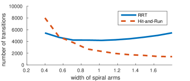
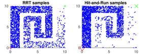
RRT is slow in this problem because in many rounds the tree does not grow in the right direction. For example at the beginning the tree needs to grow upwards, but most random samples will bias the growth to right. As Hit-and-Run only considers the space that is visible to the current point, it is less sensitive to the geometry of the free space. We can make this problem arbitrarily hard for RRT by making the middle part of the spiral fatter. Hit-and-Run, on the other hand, is insensitive to such changes. Additionally, the growth of the RRT tree can become very slow towards the end. This is because the rest of the tree absorbs most samples, and the tree grows only if the random point falls in the vicinity of the goal.

4.2 Kinematic Planning

In this set of simulations, we constrain the state transitions to adhere to the laws of physics: the state propagates forward under kinematics until it exits the permissible map, in which case it stops inelastically at the boundary. The position map is the two-turn corridor, illustrated in the bottom plots of Figure 3. Both algorithms propose points to in the analogous manner to the previous section (where a desired speed is sampled in addition to a desired position); then, the best acceleration vector in the unit ball is calculated and the sample is propagated forward by the kinematics. If the sample point encounters the boundary, the velocity is zeroed. Both RRT and Hit-and-Run are constrained to use the same controller and the only difference is what points are proposed.

Figure 3: Performance under kinematic constraints

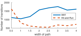
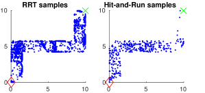
We see that Hit-and-Run again outperforms RRT across a large gamut of path widths by as much as a factor of three. The bottom two plots are of a typical sample path, and we see that Hit-and-Run has two advantages: it accelerates down straight hallways, and it samples more uniformly from the state space. In contrast, RRT wastes many more samples along the boundaries.

5 Conclusions and Future Work

This paper has two main contributions. First, we use a measure-preserving bilipschitz map to extend the analysis of the Hit-and-Run random walk to non-convex sets. Mixing time bounds for non-convex sets open up many applications, for example non-convex optimization via simulated annealing and similar methods. The second contribution of this paper has been to study one such application: the planning problem.

In contrast to RRT, using Hit-and-Run for planning has stronger guarantees on the number of samples needed and faster convergence in some cases. It also avoids the need for a sampling oracle for $\Sigma$, since it combines the search with an approximate sampling oracle. One drawback is that the sample paths for Hit-and-Run have no pruning and are therefore longer than the RRT paths. Hybrid approaches that yield short paths but also explore quickly are a promising future direction.

Appendix A Proofs

(a) The geometry used in Lemma 11.

(b) The geometry used in Lemma 11.

Figure 4: If two points are close to each other, they have similar views.

Proof of Lemma 11.

We say a line segment $L$ is not fully visible from a point $x$ if there exists a point on the line segment that is not visible from $x$. We denote this event by $L\notin\textsc{view}(x)$. Let $L$ be a line segment chosen by Hit-and-Run from $u$. So, as the next point in the Markov chain, Hit-and-Run chooses a point uniformly at random from $L$. We know that

$$P_{u}(\{x:x\notin\textsc{view}(v)\})\leq P_{u}(\{L:L\notin\textsc{view}(v)\})\,,$$

So it suffices to show

$$P_{u}(\{L:L\notin\textsc{view}(v)\})\leq\max\left(\frac{4}{\pi},\frac{\kappa}{\sin(\pi/8)}\right)\frac{\epsilon^{\prime}}{\epsilon}\;.$$ (7)

To sample the line segment $L$, first we sample a random two dimensional plane containing $u$ and $v$, and then sample the line segment inside this plane. To prove (7), we show that in any two dimensional plane containing $u$ and $v$, the ratio of invisible to visible region is bounded by $\max\left(\frac{4}{\pi},\frac{\kappa}{\sin(\pi/8)}\right)\frac{\epsilon^{\prime}}{\epsilon}$.color=blue!20!white,]Victor: be sure the plane argument is not fishy

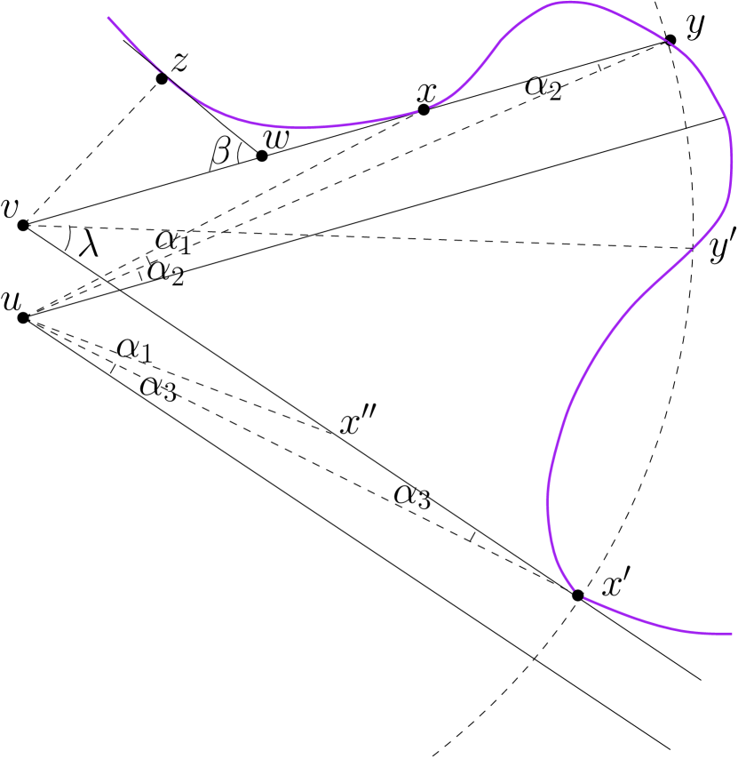
Consider the geometry shown in Figure 4(a). Let ${\cal H}$ be the intersection of $\partial\Sigma$ and a two dimensional plane containing $u$ and $v$. For a line $\ell$ and points $q$ and $u$, we write $[q,\ell,u]$ to denote that $u$ and a small neighborhood of $q$ on ${\cal H}$ are on the opposite sides of $\ell$. For example, in Figure 4(a), we have that $[x,\ell(v,x),u]$. Define a subset

$$Q=\{q\in{\cal H}\,:\,\ell(v,q)\mbox{ is tangent to }{\cal H}\mbox{ at }q\mbox{ and }[q,\ell(v,q),u]\}\;.$$

Any line $\ell(v,q)$ such that $[q,\ell(v,q),u]$ creates some space that is visible to $u$ and invisible to $v$. If $Q$ is empty, then the entire ${\cal H}$ is in the view of $v$ and $P_{u}(\{x:x\notin\textsc{view}(v)\})=0$.color=blue!20!white,]Victor: Can you make this claim formal? Otherwise, let $x$ be a member of $Q$. Let $y\in{\cal H}$ be the closest point to $x$ such that $[v,y]$ is tangent to ${\cal H}$ at $x$. Let $\alpha_{1}$ be the angle between $[x,u]$ and $[u,y]$, and let $\alpha_{2}$ be the angle between $[y,v]$ and $[y,u]$. Because $\left|u-v\right|\leq\left|v-z\right|\leq\left|v-x\right|$, $\alpha_{1}+\alpha_{2}\leq\pi/2$. Further, if the lengths of $\left|u-v\right|$ and $\left|v-x\right|$ are fixed, $\alpha_{1}+\alpha_{2}$ is maximized when $[v,u]$ is orthogonal to $[u,x]$. If $x$ is the only member of $Q$, then maximum invisible angle is $\alpha_{1}$, which can be bounded as follows:

$$\sin\alpha_{1}\leq\sin(\alpha_{1}+\alpha_{2})\leq\frac{\left|u-v\right|}{\left|v-x\right|}\leq\frac{\left|u-v\right|}{\epsilon}\;.$$

Otherwise, assume $Q$ has more members. The same upper bound holds for members that are also on the line $\ell(v,x)$. So next we consider members of $Q$ that are not on the line $\ell(v,x)$. Assume $Q$ has only one such member and let $x^{\prime}$ be that tangent point (see Figure 4(a). The same argument can be repeated if $Q$ has more such members). We consider two cases. Case 1: $\left|v-x^{\prime}\right|\geq\left|v-y\right|$. Let $\alpha_{3}$ be the angle between $[v,x^{\prime}]$ and $[u,x^{\prime}]$. If $\alpha_{3}\leq\alpha_{2}$, then

$$\sin(\alpha_{1}+\alpha_{3})\leq\sin(\alpha_{1}+\alpha_{2})\leq\frac{\left|u-v\right|}{\epsilon}\;.$$

Otherwise, $\alpha_{3}>\alpha_{2}$. Consider point $x^{\prime\prime}$ such that the angle between $[u,x^{\prime}]$ and $[u,x^{\prime\prime}]$ is $\alpha_{1}$. We show that $\left|v-x^{\prime\prime}\right|\geq\left|v-x\right|$ by contradiction. Assume $\left|v-x\right|>\left|v-x^{\prime\prime}\right|$. Thus, $\left|x^{\prime}-x^{\prime\prime}\right|>\left|y-x\right|$ and $\left|u-x\right|>\left|u-x^{\prime\prime}\right|$. By law of sines, $\left|x-y\right|/\sin\alpha_{1}=\left|u-x\right|/\sin\alpha_{2}$ and $\left|x^{\prime\prime}-x^{\prime}\right|/\sin\alpha_{1}=\left|u-x^{\prime\prime}\right|/\sin\alpha_{3}$. Because $\left|u-x\right|>\left|u-x^{\prime\prime}\right|$ and $\alpha_{3}>\alpha_{2}$, we have that $\left|u-x\right|/\sin\alpha_{2}>\left|u-x^{\prime\prime}\right|/\sin\alpha_{3}$, and thus $\left|x^{\prime\prime}-x^{\prime}\right|/\sin\alpha_{1}<\left|x-y\right|/\sin\alpha_{1}$. This implies $\left|x^{\prime\prime}-x^{\prime}\right|<\left|x-y\right|$, a contradiction. color=blue!20!white,]Victor: add argument to have u on the right side of vcolor=red!20!white,]Yasin: the new definition of $Q$ ensures that $u$ is in the right side. Thus,

$$\sin(\alpha_{1}+\alpha_{3})\leq\frac{\left|u-v\right|}{\left|v-x^{\prime\prime}\right|}\leq\frac{\left|u-v\right|}{\left|v-x\right|}\leq\frac{\left|u-v\right|}{\epsilon}\;.$$

Next we consider the second case. Case 2: $\left|v-x^{\prime}\right|<\left|v-y\right|$. Consider the arc on ${\cal H}$ from $y$ to $x^{\prime}$. Let $y^{\prime}$ be the last point on this arc such that $\left|v-y^{\prime}\right|=\left|v-y\right|$. Let $\eta$ be the change of angle between the tangent of ${\cal H}$ at $y^{\prime}$ and the tangent of ${\cal H}$ at $x^{\prime}$ (tangents are defined in clockwise direction), and let $\lambda$ be the angle between $[v,y^{\prime}]$ and $[v,x^{\prime}]$. Angle $\eta$ is minimized color=blue!20!white,]Alan: I don’t see why this is truecolor=red!20!white,]Yasin: Notice that $y^{\prime}$ is the last point on this arc such that $\left|v-y^{\prime}\right|=\left|v-y\right|$. So the angle between $[y^{\prime},v]$ and the tangent at $y^{\prime}$ is less than $\pi/2$.color=blue!20!white,]Victor: define angles between lines properly as two opposite choices can be made when the tangent at $y^{\prime}$ is orthogonal to $[v,y^{\prime}]$. Thus $\eta\geq\pi/2-\lambda$. If $\lambda<\pi/4$, then $\eta\geq\pi/4$. Angle $\lambda$ is smallest when the arc from $y^{\prime}$ to $x^{\prime}$ changes with maximum curvature $\kappa/{\cal R}_{\cal H}$, i.e. it is a segment of a circle with radius ${\cal R}_{\cal H}/\kappa$. Figure 4(b) shows this case, where $R={\cal R}_{\cal H}/\kappa$ and $L=\left|v-y^{\prime}\right|$. We have that

$$\frac{\sin(\lambda/2)}{\sin(\eta/2)}\geq\frac{h/L}{h/R}=\frac{R}{L}=\frac{{\cal R}_{\cal H}}{\kappa\left|v-y\right|}$$

Thus,

$$\frac{\lambda}{2}\geq\sin(\lambda/2)\geq\frac{{\cal R}_{\cal H}}{\kappa\left|v-y\right|}\sin(\eta/2)=\frac{\sin(\pi/8){\cal R}_{\cal H}}{\kappa\left|v-y\right|}\geq\frac{\sin(\pi/8)}{\kappa}\,,$$

where the last step follows by $\left|v-y\right|\leq{\cal R}_{\cal H}$. Thus

$$\lambda\geq\lambda_{0}\stackrel{{\scriptstyle\mbox{\rm\tiny def}}}{{=}}\min\left(\frac{\pi}{4},\frac{\sin(\pi/8)}{\kappa}\right)\;.$$

So for every $\left|u-v\right|/\epsilon$ invisible region, we have at least $\lambda_{0}$ visible region. Thus,

$$P_{u}(\{x:x\notin\textsc{view}(v)\})\leq\frac{\left|u-v\right|}{\lambda_{0}\epsilon}=\max\left(\frac{4}{\pi},\frac{\kappa}{\sin(\pi/8)}\right)\frac{\left|u-v\right|}{\epsilon}\;.$$

∎

Before proving Lemma 12, we show a useful inequality. Consider points $u,v,w\in\Sigma$ that see each other. Let ${\cal C}$ be the convex hull of

$$\{a(u,v),b(u,v),a(u,w),b(u,w),a(v,w),b(v,w)\}\;.$$

Let $i$ and $j$ be distinct members of $\{u,v,w\}$. We use $a^{\prime}(i,j)$ and $b^{\prime}(i,j)$ to denote the endpoints of $\ell_{{\cal C}}(i,j)$ that are closer to $i$ and $j$, respectively. Because $\left|a^{\prime}(i,j)-b^{\prime}(i,j)\right|$ is convex combination of two line segments that are inside $\Sigma$,

$$\left|a^{\prime}(i,j)-b^{\prime}(i,j)\right|\leq D_{\Sigma}\;.$$ (8)

Also $[a(i,j),b(i,j)]\subset[a^{\prime}(i,j),b^{\prime}(i,j)]$, and thus $\left|a(i,j)-i\right|\leq\left|a^{\prime}(i,j)-i\right|$ and $\left|b(i,j)-j\right|\leq\left|b^{\prime}(i,j)-j\right|$. We can write

$$\ell_{\cal C}(i,j) =\frac{\left|i-j\right|\cdot\left|a^{\prime}(i,j)-b^{\prime}(i,j)\right|}{\left|a^{\prime}(i,j)-i\right|\cdot\left|j-b^{\prime}(i,j)\right|}$$

$$\leq\frac{\left|i-j\right|\cdot\left|a(i,j)-b(i,j)\right|}{\left|a(i,j)-i\right|\cdot\left|j-b(i,j)\right|}\cdot\frac{\left|a^{\prime}(i,j)-b^{\prime}(i,j)\right|}{\left|a(i,j)-b(i,j)\right|}$$

$$\leq D_{\Sigma}\frac{\ell_{\Sigma}(i,j)}{d(i,\partial\Sigma)}\,,$$ (9)

where the last inequality holds because $\left|a(i,j)-b(i,j)\right|\geq d(i,\partial\Sigma)$.

Proof of Lemma 12.

Let $A\subset\Sigma$ be a measurable subset of $\Sigma$. We prove that

$$P_{u}(A)-P_{v}(A)\leq 1-\frac{\epsilon}{8e^{4}D_{\Sigma}}\;.$$

color=blue!20!white,]Alan: needs $|\cdot|$? color=red!20!white,]Yasin: no! We partition $A$ into five subsets, and estimate the probability of each of them separately:

$$A_{1} =\left\{x\in A\,:\,\left|x-u\right|<F(u)\right\}\,,$$

$$A_{2} =\left\{x\in A\,:\,\left|(x-u)^{\top}(u-v)\right|>\frac{1}{\sqrt{n}}\left|x-u\right|\cdot\left|u-v\right|\right\}\,,$$

$$A_{3} =\Bigg{\{}x\in A\,:\,\left|x-u\right|<\frac{1}{6}\left|u-a(u,x)\right|\,,$$

$$\qquad\qquad\qquad\mbox{ or }\left|x-u\right|<\frac{1}{6}\left|u-a(x,u)\right|\Bigg{\}}\,,$$

$$A_{4} =\left\{x\in A\,:\,x\in\textsc{view}(u),\,x\notin\textsc{view}(v)\right\}\,,$$

$$S =A\setminus A_{1}\setminus A_{2}\setminus A_{3}\setminus A_{4}\;.$$

The definition of $F(u)$ immediately yields $P_{u}(A_{1})\leq 1/8$. Now consider $A_{2}$ and let $C$ be the cap of the unit sphere centered at $u$ in the direction of $v$, defined by $C=\{x:(u-v)^{\top}x\geq\frac{1}{\sqrt{n}}|u-v|\}$. If $x\sim P_{u}$, then $P(x\in A_{2})$ is bounded above by the probability that a uniform random line through $u$ intersects $C$, which has probability equal to the ratio between the surface of $C$ and the surface of the half-sphere. A standard computation to show that this ratio is less than $1/6$, and hence $P_{u}(A_{2})\leq 1/6$. The probability that $x\in A_{3}$ is at most $1/6$, since $x$ is chosen from a segment of a chord of length at most $|\ell(u,x)|/6$. Finally, to bound $P(A_{4})$, we apply Lemma 11:

$$P_{u}\left(x\in A\,:\,x\in\textsc{view}(u),\,x\notin\textsc{view}(v)\right)\leq\max\left(\frac{4}{\pi},\frac{\kappa}{\sin(\pi/8)}\right)\frac{\epsilon^{\prime}}{\epsilon}\leq\frac{1}{6}\;.$$

The combined probability of $A_{1},A_{2},A_{3}$, and $A_{4}$ is at most $1/8+1/6+1/6+1/6<3/4$.

We now turn to bounding $P_{u}(S)$ and show that $P_{u}(S)\leq 2e^{4}(D_{\Sigma}/\epsilon)P_{v}(S)$. Because points in $S$ are visible from both $u$ and $v$, by (2)

$$P_{v}(S)=\frac{2}{n\pi_{n}}\int_{S}\frac{1}{\ell_{\Sigma}(v,x)\left|x-v\right|^{n-1}}\;.$$

Now, any $x\in S$ must respect the following

$$\left|x-u\right| \geq F(u)\geq\frac{\sqrt{n}}{2}\left|u-v\right|\,,$$ (10)

$$\left|(x-u)^{\top}(u-v)\right| \leq\frac{1}{\sqrt{n}}\left|x-u\right|\cdot\left|u-v\right|\,,$$ (11)

$$\left|x-u\right| \geq\frac{1}{6}\left|u-a(u,x)\right|,\text{ and }$$ (12)

$$\left|x-u\right| \geq\frac{1}{6}\left|u-a(x,u)\right|\;.$$ (13)

Figure 5: Illustration for Lemma 12 proof

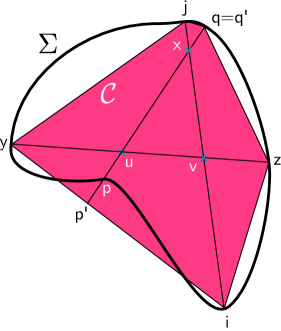
As illustrated in Figure 5, we define the points $y=a(u,v)$, $z=a(v,u)$, $p=a(u,x)$, $q=a(x,u)$, $i=a(v,x)$ and $j=a(x,v)$ with convex hull ${\cal C}$. Also let $p^{\prime}$ and $q^{\prime}$ be the endpoints of $\ell_{\cal C}(u,x)$. If $p^{\prime}=p$ and $q^{\prime}=q$, we proceed with the argument in the proof of Lemma 9 of Lovász (1999) to get the desired result. Otherwise, assume $q^{\prime}=q$ and $p^{\prime}$ is the intersection of the lines $\ell(u,p)$ and $\ell(y,i)$. (See Figure 5. A similar argument holds when $q\neq q^{\prime}$.) From (12) and (13), we get that

$$2\left|x-u\right|>\frac{1}{6}\left|p-q\right|\;.$$

We have that $\left|p-q\right|\geq\epsilon$, and by (8), $\left|p^{\prime}-q^{\prime}\right|\leq D_{\Sigma}$. Thus $\left|p^{\prime}-q^{\prime}\right|\leq(D_{\Sigma}/\epsilon)\left|p-q\right|$. Thus,

$$\frac{1}{6}\left|p^{\prime}-q^{\prime}\right|\leq\frac{2D_{\Sigma}}{\epsilon}\left|x-u\right|\;.$$ (14)

To relate $P_{v}(S)$ to $P_{u}(S)$, we need to bound $\left|x-v\right|$ and $\ell(x,v)$ in terms of $\left|x-u\right|$ and $\ell(x,u)$:

$$\left|x-v\right|^{2} =\left|x-u\right|^{2}+\left|u-v\right|^{2}+2(x-u)^{\top}(u-v)$$

$$\leq\left|x-u\right|^{2}+\left|u-v\right|^{2}+\frac{2}{\sqrt{n}}\left|x-u\right|\cdot\left|u-v\right|$$ …By (11)

$$\leq\left|x-u\right|^{2}+\frac{4}{n}\left|x-u\right|^{2}+\frac{4}{n}\left|x-u\right|^{2}$$ …By (10)

$$=\left(1+\frac{8}{n}\right)\left|x-u\right|^{2}\;.$$

Thus,

$$\left|x-v\right|\leq\left(1+\frac{4}{n}\right)\left|x-u\right|\;.$$ (15)

First we use convexity of ${\cal C}$ to bound $\ell_{\cal C}(x,v)$ in terms of $\ell_{\cal C}(x,u)$, and then we use (9) to bound $\ell_{\Sigma}(x,v)$ and $\ell_{\Sigma}(x,u)$ in terms of $\ell_{\cal C}(x,v)$ and $\ell_{\cal C}(x,u)$. By Menelaus’ Theorem (wrt triangle $uvx$ and transversal line $[y,i]$),

$$\frac{\left|x-i\right|}{\left|v-i\right|}=\frac{\left|u-y\right|}{\left|v-y\right|}\cdot\frac{\left|x-p^{\prime}\right|}{\left|u-p^{\prime}\right|}\;.$$

We have that

$$\frac{\left|u-y\right|}{\left|v-y\right|}=1-\frac{\left|v-u\right|}{\left|v-y\right|}>1-d_{\cal C}(u,v)\,,$$

and thus

$$\frac{\left|x-v\right|}{\left|v-i\right|} =\frac{\left|x-i\right|}{\left|v-i\right|}-1$$

$$\geq(1-d_{\cal C}(u,v))\frac{\left|x-p^{\prime}\right|}{\left|u-p^{\prime}\right|}-1$$

$$=\frac{\left|x-u\right|}{\left|u-p^{\prime}\right|}\left(1-d_{\cal C}(u,v)\frac{\left|x-p^{\prime}\right|}{\left|x-u\right|}\right)$$

$$>\frac{\left|x-u\right|}{\left|u-p^{\prime}\right|}\left(1-d_{\cal C}(u,v)\frac{\left|p^{\prime}-q^{\prime}\right|}{\left|x-u\right|}\right)$$

$$>\frac{\left|x-u\right|}{\left|u-p^{\prime}\right|}\left(1-\frac{12D_{\Sigma}\epsilon}{24D_{\Sigma}\epsilon}\right)$$

$$>\frac{1}{2}\frac{\left|x-u\right|}{\left|u-p^{\prime}\right|}\,,$$

where we have used (14) and $d_{\cal C}(u,v)=d_{\Sigma}(u,v)<\epsilon/(24D_{\Sigma})$ (the condition in the statement of the lemma); we conclude that

$$\left|v-i\right|<2\frac{\left|x-v\right|}{\left|x-u\right|}\left|u-p^{\prime}\right|\;.$$ (16)

Next we prove a similar inequality for $\left|v-j\right|$. It is easy to check that

$$\frac{\left|z-v\right|}{\left|u-z\right|}=1-\frac{\left|u-v\right|}{\left|u-z\right|}>1-d_{\cal C}(u,v)\,,$$

and combining with Menelaus’ Theorem

$$\frac{\left|v-j\right|}{\left|x-j\right|}=\frac{\left|q^{\prime}-u\right|}{\left|x-q^{\prime}\right|}\cdot\frac{\left|z-v\right|}{\left|u-z\right|}$$

we can show

$$\frac{\left|x-v\right|}{\left|x-j\right|} =\frac{\left|v-j\right|}{\left|x-j\right|}-1$$

$$\geq(1-d_{\cal C}(u,v))\frac{\left|q^{\prime}-u\right|}{\left|x-q^{\prime}\right|}-1$$

$$=\frac{\left|x-u\right|}{\left|x-q^{\prime}\right|}\left(1-d_{\cal C}(u,v)\frac{\left|q^{\prime}-u\right|}{\left|x-u\right|}\right)$$

$$>\frac{\left|x-u\right|}{\left|x-q^{\prime}\right|}\left(1-d_{\cal C}(u,v)\frac{\left|p^{\prime}-q^{\prime}\right|}{\left|x-u\right|}\right)$$

$$>\frac{\left|x-u\right|}{\left|x-q^{\prime}\right|}\left(1-\frac{12D_{\Sigma}\epsilon}{24D_{\Sigma}\epsilon}\right)$$

$$>\frac{1}{2}\frac{\left|x-u\right|}{\left|x-q^{\prime}\right|}\,,$$

where we have used (14) and $d_{\cal C}(u,v)=d_{\Sigma}(u,v)<\epsilon/(24D_{\Sigma})$. Thus,

$$\left|x-j\right|<2\frac{\left|x-v\right|}{\left|x-u\right|}\left|x-q^{\prime}\right|\;,$$

and combining this with the trivial observation that $\left|x-v\right|\leq 2\frac{\left|x-v\right|}{\left|x-u\right|}\left|x-u\right|\,,$ and Equation 16 yields

$$\ell_{\cal C}(x,v)=\left|v-i\right|+\left|v-x\right|+\left|x-j\right|\leq 2\frac{\left|x-v\right|}{\left|x-u\right|}\ell_{\cal C}(x,u)\;.$$

Thus,

$$\ell_{\Sigma}(x,v) =\ell_{\cal C}(x,v)$$

$$\leq 2\frac{\left|x-v\right|}{\left|x-u\right|}\ell_{\cal C}(x,u)$$

$$\leq\frac{2D_{\Sigma}}{\epsilon}\frac{\left|x-v\right|}{\left|x-u\right|}\ell_{\Sigma}(x,u)\;.$$ (17)

Where the last step holds by (9). Now we are ready to lower bound $P_{v}(S)$ in terms of $P_{u}(S)$.

$$P_{v}(S) =\frac{2}{n\pi_{n}}\int_{S}\frac{dx}{\ell_{\Sigma}(x,v)\left|x-v\right|^{n-1}}$$

$$\geq\frac{\epsilon}{n\pi_{n}D_{\Sigma}}\int_{S}\frac{\left|x-u\right|dx}{\ell_{\Sigma}(x,u)\left|x-v\right|^{n}}$$ …By (17)

$$\geq\frac{\epsilon}{n\pi_{n}D_{\Sigma}}\left(1+\frac{4}{n}\right)^{-n}\int_{S}\frac{dx}{\ell_{\Sigma}(x,u)\left|x-u\right|^{n-1}}$$ …By (15)

$$\geq\frac{\epsilon}{2e^{4}D_{\Sigma}}P_{u}(S)\;.$$

Finally,

$$P_{u}(A)-P_{v}(A) \leq P_{u}(A)-P_{v}(S)$$

$$\leq P_{u}(A)-\frac{\epsilon}{2e^{4}D_{\Sigma}}P_{u}(S)$$

$$\leq P_{u}(A)-\frac{\epsilon}{2e^{4}D_{\Sigma}}\left(P_{u}(A)-\frac{3}{4}\right)$$

$$=\frac{3\epsilon}{8e^{4}D_{\Sigma}}+\left(1-\frac{\epsilon}{2e^{4}D_{\Sigma}}\right)P_{u}(A)$$

$$\stackrel{{\scriptstyle(a)}}{{\leq}}\frac{3\epsilon}{8e^{4}D_{\Sigma}}+1-\frac{4\epsilon}{8e^{4}D_{\Sigma}}$$

$$=1-\frac{\epsilon}{8e^{4}D_{\Sigma}}\;.$$

In the step (a), we used the fact that $D_{\Sigma}\geq\epsilon$ and $P_{u}(A)\leq 1$. ∎

Proof of Lemma 13.

Let $\{S_{1},S_{2}\}$ be a partitioning of $\Sigma$. Define

$$\Sigma_{1} =\left\{x\in S_{1}\ :\ P_{x}(S_{2})\leq\delta\right\}\,,$$

$$\Sigma_{2} =\left\{x\in S_{2}\ :\ P_{x}(S_{1})\leq\delta\right\}\,,$$

$$\Sigma_{3} =\Sigma\setminus\Sigma_{1}\setminus\Sigma_{2}\;.$$

Case 1: $\textsc{vol}(\Sigma_{1})\leq\textsc{vol}(S_{1})/2$. We have that

$$\int_{S_{1}}P_{x}(S_{2})dx \geq\int_{S_{1}\setminus\Sigma_{1}}P_{x}(S_{2})dx\geq\delta\textsc{vol}(S_{1}\setminus\Sigma_{1})\geq\frac{\delta}{2}\textsc{vol}(S_{1})\;.$$

Thus,

$$\frac{1}{\min\{\textsc{vol}(S_{1}),\textsc{vol}(S_{2})\}}\int_{S_{1}}P_{x}(S_{2})dx \geq\frac{\delta}{2}\;.$$

Case 2: $\textsc{vol}(\Sigma_{1})>\textsc{vol}(S_{1})/2$ and $\textsc{vol}(\Sigma_{2})>\textsc{vol}(S_{2})/2$. Similar to the argument in the previous case,

$$\int_{S_{1}}P_{x}(S_{2})\geq\delta\,\textsc{vol}(S_{1}\setminus\Sigma_{1})\,,$$

and

$$\int_{S_{1}}P_{x}(S_{2})=\int_{S_{2}}P_{x}(S_{1})\geq\delta\,\textsc{vol}(S_{2}\setminus\Sigma_{2})\;.$$

Thus,

$$\int_{S_{1}}P_{x}(S_{2})\geq\frac{\delta}{2}\,\textsc{vol}(\Sigma\setminus\Sigma_{1}\setminus\Sigma_{2})=\frac{\delta}{2}\,\textsc{vol}(\Sigma_{3})\;.$$

Let $\Omega_{i}=g^{-1}(\Sigma_{i})$ for $i=1,2,3$. Define

$$(u(x),v(x))=\mathop{\rm argmin}_{u\in\Omega_{1},v\in\Omega_{2},\{u,v,x\}\text{ are collinear}}d_{\Omega}(u,v)\,,\qquad h(x)=(1/3)\min(1,d_{\Omega}(u(x),v(x)))\;.$$

By definition, $h(x)$ satisfies condition of Theorem 7. Let $\epsilon=\frac{r}{2n}$ and notice that $\textsc{vol}(\Omega^{\epsilon})\geq\textsc{vol}(\Omega)/2$. We have that

$$\int_{S_{1}}P_{x}(S_{2}) \geq\frac{\delta}{2}\,\textsc{vol}(\Omega_{3})$$

$$\geq\frac{\delta}{2}\mathbf{E}_{\Omega}(h(x))\min(\textsc{vol}(\Omega_{1}),\textsc{vol}(\Omega_{2}))$$

$$=\frac{\delta}{4}\mathbf{E}_{\Omega^{\epsilon}}(h(x))\min(\textsc{vol}(\Sigma_{1}),\textsc{vol}(\Sigma_{2}))\;.$$

Let $x\in\Omega^{\epsilon}$. We consider two cases. In the first case, $\left|u(x)-v(x)\right|\geq\epsilon/10$. Thus,

$$d_{\Omega}(u(x),v(x))\geq\frac{4}{D_{\Omega}}\left|u(x)-v(x)\right|\geq\frac{2}{5nD_{\Omega}}\;.$$

In the second case, $\left|u(x)-v(x)\right|<\epsilon/10$, then $\left|u(x)-x\right|\leq\epsilon/10$ and $\left|v(x)-x\right|\leq\epsilon/10$. Thus, $u,v\in\Omega^{\epsilon^{\prime}}$ for $\epsilon^{\prime}=9\epsilon/10$. Thus by Assumption 2, $g(u),g(v)\in\Sigma^{\epsilon^{\prime\prime}}$ for $\epsilon^{\prime\prime}=9\epsilon/(10L_{\Omega})$. By Lemma 10,

$$d_{\Omega}(u(x),v(x))\geq\frac{\widetilde{d}_{\Sigma}(g(u(x)),g(v(x)))}{4L_{\Sigma}^{2}L_{\Omega}^{2}R_{\epsilon^{\prime}}(1+2R_{\epsilon^{\prime}})}\;.$$

Next we lower bound $\widetilde{d}_{\Sigma}(g(u),g(v))$. If $g(u)$ and $g(v)$ cannot see each other, then $\widetilde{d}_{\Sigma}(g(u),g(v))\geq 8\epsilon^{\prime\prime}/D_{\Sigma}$. Next we assume that $g(u)$ and $g(v)$ see each other. Because $g(u)\in\Sigma_{1}$ and $g(v)\in\Sigma_{2}$,

$$d_{tv}(P_{g(u)}-P_{g(v)})\geq 1-P_{g(u)}(S_{2})-P_{g(v)}(S_{1})\geq 1-2\delta=1-\frac{\epsilon^{\prime\prime}}{8e^{4}D_{\Sigma}}\;.$$

Lemma 12, applied to $g(u),g(v)\in\Sigma^{\epsilon^{\prime\prime}}$, gives us that

$$d_{\Sigma}(g(u),g(v))\geq\frac{\epsilon^{\prime\prime}}{24D_{\Sigma}}\qquad\mbox{or}\qquad\left|g(u)-g(v)\right|\geq\frac{2}{\sqrt{n}}\min\left(\frac{2F(g(u))}{\sqrt{n}},G\epsilon^{\prime\prime}\right)\;.$$

By (6), $F(g(u))\geq\epsilon^{\prime\prime}/16$. We get the desired lower bound by taking a minimum over all cases. ∎

References

- Abbasi-Yadkori et al. (2010) Y. Abbasi-Yadkori, J. Modayil, and Cs. Szepesvari. Extending rapidly-exploring random trees for asymptotically optimal anytime motion planning. In International Conference on Intelligent Robots and Systems (IROS), 2010.
- Chandrasekaran et al. (2010) Karthekeyan Chandrasekaran, Daniel Dadush, and Santosh Vempala. Thin partitions: Isoperimetric inequalities and sampling algorithms for some nonconvex families. In ACM-SIAM Symposium on Discrete Algorithms (SODA), 2010.
- Fonseca and Parry (1992) I. Fonseca and G. Parry. Equilibrium configurations of defective crystals. Arch. Rational Mech. Anal., 120:245–283, 1992.
- Griepentrog et al. (2008) J. A. Griepentrog, W. Höppner, H-C. Kaiser, and J. Rehberg. A bi-lipschitz continuous, volume preserving map from the unit ball onto a cube. Note di Matematica, 28:177–193, 2008.
- Karaman and Frazzoli (2010) S. Karaman and E. Frazzoli. Incremental sampling-based algorithms for optimal motion planning, 2010.
- Karaman and Frazzoli (2011) Sertac Karaman and Emilio Frazzoli. Sampling-based algorithms for optimal motion planning. International Journal of Robotics Research., 30(7):846–894, 2011.
- LaValle (1998) Steven M. LaValle. Rapidly-exploring random trees: A new tool for path planning. Technical Report TR 98-11, Computer Science Department, Iowa State University, 1998.
- LaValle and Kuffner Jr. (2001) Steven M. LaValle and James J. Kuffner Jr. Randomized kinodynamic planning. The International Journal of Robotics Research, 20(5), 2001.
- Lovász (1999) László Lovász. Hit-and-run mixes fast. Mathematical Programming, 86(3):443–461, 1999.
- Lovász and Simonovits (1993) László Lovász and Miklós Simonovits. Random walks in a convex body and an improved volume algorithm. Random Structures and Algorithms, 4(4):359–412, 1993.
- Lovász and Vempala (2006) László Lovász and Santosh Vempala. Hit-and-run from a corner. SIAM Journal on Computing, 35(4):985–1005, 2006.
- Lovász and Vempala (2007) László Lovász and Santosh Vempala. The geometry of logconcave functions and sampling algorithms. Random Structures & Algorithms, 30(3):307–358, 2007.
- Smith (1984) R.L. Smith. Efficient monte-carlo procedures for generating points uniformly distributed over bounded regions. Operation Research, 32:1296–1308, 1984.
- Vempala (2005) Santosh Vempala. Geometric random walks: A survey. Combinatorial and Computational Geometry, 52, 2005.