Nonparametric modal regression in the presence of measurement error
Abstract
In the context of regressing a response on a predictor , we consider estimating the local modes of the distribution of given when is prone to measurement error. We propose two nonparametric estimation methods, with one based on estimating the joint density of in the presence of measurement error, and the other built upon estimating the conditional density of given using error-prone data. We study the asymptotic properties of each proposed mode estimator, and provide implementation details including the mean-shift algorithm for mode seeking and bandwidth selection. Numerical studies are presented to compare the proposed methods with an existing mode estimation method developed for error-free data naively applied to error-prone data.
doi:
10.1214/154957804100000000keywords:
[class=MSC]keywords:
and
1 Introduction
The majority of statistical literature on regression analysis focuses on inferring the mean function of the response given a predictor . There are also a large body of work devoted to making inference for the quantiles of given in the regression setting (e.g., Koenker, 2005). Recently, researchers started to investigate methods to infer local modes of given (see Yao et al., 2012; Yao and Li, 2014; Chen et al., 2016, among others). These researchers pointed out valuable information about the association between the response and the predictor that conditional modes can provide yet the conditional mean/quantiles can miss. Advantages of modal regression compared to mean or quantile regression have been well appreciated in analyzing speed-flow data in traffic engineering (Einbeck and Tutz, 2006), studying temperature patterns (Hyndman et al., 1996), investigating galaxy properties conditioning on a given environment (Bamford et al., 2008), and in economics (Huang et al., 2013) for instance. To address the practical issue of error-contaminated covariates, methods accounting for measurement error in mean regression (Carroll et al., 2006) and methods for quantile regression in the presence of measurement error (He and Liang, 2000; Wei and Carroll, 2009; Ma and Yin, 2011; Wang et al., 2012) have been developed. In contrast, there is no existing research on modal regression when is prone to measurement error even though this issue often arises in the aforementioned applications, and ignoring measurement error in modal regression typically results in misleading inference. We tackle this important problem in our study.
We propose two nonparametric methods for estimating conditional modes of a response variable given an error-prone covariate . The first method exploits a kernel density estimator of the joint density of that accounts for measurement error in . The second method is based on a local linear estimator of the conditional density of given . These methods are elaborated in Section 2. Asymptotic properties of the mode estimators resulting from these methods are presented in Section 3. We provide a data-driven method for bandwidth selection to facilitate the implementation of the proposed methods in Section 4. Numerical studies are presented in Section 5, which include simulation experiments and an application to dietary data. Section 6 provides a discussion on follow-up open research questions.
2 Nonparametric estimation of local modes
2.1 Data and measurement error model
Suppose one wishes to collect data for a response and a covariate ,
, consisting of independent pairs from a bivariate distribution specified by the joint probability density function (pdf), . However, the reality is that cannot be observed directly due to error contamination, and are observed instead. More specifically, the observed covariate relates to the underlying true covariate via an additive measurement error model given by
| (2.1) |
where are nondifferential measurement errors (Carroll et al., 2006, Section 2.5), meaning that and . We assume a known distribution of specified by its pdf in this study. Estimating the distribution of requires either replicate measures of each underlying or external validation data. For instance, if replicate measures are available and one assumes known up to some parameters, such as the variance parameter, then one can follow equation (4.3) in Carroll et al. (2006) to estimate the measurement error variance consistently. One may also estimate the characteristic function of as proposed in Delaigle et al. (2008), which is all our proposed inference methods need in terms of information regarding the measurement error distribution.
The focal point of statistical inference presented in this study lies in local modes of the conditional pdf of given , . Denote by the support of and by the support of . For a generic bivariate function , refers to evaluated at , and notations for higher-order partial derivatives of are similarly defined. Given , a mode of , denoted by , is a value in such that and . Equivalently, satisfies and . This latter viewpoint motivates our first proposed estimator of described next. It is possible that is multimodal at a given , producing a mode set . Although multi-modality brings in certain challenges in the actual implementation of mode seeking, it adds little complication in asymptotics analyses of our proposed mode estimators. To avoid unnecessarily tedious notations, we assume a unimodal for the methodology development and theoretical analysis in the main article. We repeat the key part of the preliminary theoretical development with the uni-modality assumption relaxed in Appendix I for illustration purposes. In addition, multimodal is considered when illustrating the implementation of the proposed methods in Section 5.
Even though the conditional mode set is formulated above in terms of the joint pdf , we shall point out that, as moves in , the resultant conditional mode curve(s), , characterize the mode structure of the conditional density of given . Hence, they typically differ from density ridges (Genovese et al., 2014) and principal curves (Hastie and Stuetzle, 1989; Ozertem and Erdogmus, 2011), which focus on certain structures of the joint pdf. Chen et al. (2016, Section 8) provided detailed explanations on the distinction between conditional mode curves and density ridges, which are also helpful for one to see how they differ from principal curves.
2.2 Local constant estimator
We first consider an estimator of , denoted by , as the solution to , where is a kernel-based estimator of . The construction of traces back to the kernel density estimator of in the absence of measurement error considered in Wand and Jones (1993),
| (2.2) |
where and are bandwidths, and and are kernels. In the presence of measurement error, with observed in place of , we follow the idea of deconvoluting kernel (Carroll and Hall, 1988; Stefanski and Carroll, 1990) and propose an estimator of that accounts for measurement error as follows,
| (2.3) |
where
| (2.4) |
is the deconvoluting kernel, in which is the imaginary unit, is the Fourier transform of , and is the characteristic function of , i.e., the Fourier transform of . In this article, all integrations are over the entire real line unless otherwise specified. The estimator is motivated by the property of the deconvoluting kernel that . A direct implication of this property is that .
Differentiating (2.3) with respect to (w.r.t.) yields an estimator of based on ,
| (2.5) |
where . To facilitate mode seeking, we choose to be a radially symmetric kernel, that is, , in which is a nonnegative-valued function, referred to as the profile of , and is a positive constant serving as a normalization constant so that integrates to one. Furthermore, we choose such that its profile relates to the profile of another radially symmetric kernel via . The Epanechnikov kernel and the normal kernel are examples where a kernel possesses the above desirable features for . Using the so-chosen , (2.5) can be further elaborated as
For illustration purposes, throughout the article, we set . Then, with and , one has , with and , and the above estimator becomes
| (2.6) |
Based on in (2.6), an estimator of is the solution to the equation
Rearranging terms in this equation yields a variant of the equation leading to the following updating formula that one evaluates iteratively until convergence in order to find a solution to it,
| (2.7) |
where is the value resulting from the th iteration as an update of the value from the previous iteration, , in search for , for . One may view
as a weight associated with the th data point , for , of which the magnitude depends on the proximity of this data point to . Following this viewpoint, one can see that the right-hand side of (2.7) is a weighted average of , and one may interpret this updating formula as updating to using the weighted mean of the responses surrounding . In fact, this algorithm of finding an estimated mode is in line with the mean-shift algorithm used to search for modes of a distribution (Cheng, 1995; Comaniciu and Meer, 2002; Einbeck and Tutz, 2006; Chen et al., 2016). Compared to the existing mean-shift algorithm and its application, the complication caused by measurement error is that the weight can be negative because the deconvoluting kernel is not guaranteed to be nonnegative (Stefanski and Carroll, 1990). However, with careful choices of the bandwidths and starting values for the algorithm, as to be elaborated in Sections 4 and 5, our mean-shift algorithm can converge and produce a mode estimate .
We call the so-obtained estimator a local constant estimator of the mode because of the construction of , which in nature is a local constant estimator of . This interpretation of is made clearer when compared to the way we estimate in order to estimate the mode.
2.3 Local linear estimator
The second estimator of we propose, denoted by , is a solution to , where is an estimator of obtained as follows. We start from evoking the local linear estimator of in the absence of measurement error proposed by Fan et al. (1996) given by
| (2.8) |
where ,
in which
| (2.9) | ||||
| (2.10) |
This estimator is motivated by the property that as , and hence can be approximately viewed as the mean function when regressing on . Adopting this standpoint, one can employ the general strategy of estimating a mean function via local polynomial estimators (Fan and Gijbels, 1996) to estimate , with being the response data and as the covariate data. In particular, the local linear estimator of is as in (2.8).
In the presence of measurement error, we adjust to account for measurement error in and propose the following local linear estimator of ,
| (2.11) |
where
in which
| (2.12) | ||||
| (2.13) |
and, with denoting the -th derivative of ,
| (2.14) |
The transform of in (2.14) is a generalization of the transform in (2.4) derived in Delaigle et al. (2009). This generalization leads to a generalized deconvoluting kernel possessing the property that , . Thanks to this property, given , (2.12) and (2.13) are unbiased estimators of their counterparts in the absence of measurement error in (2.9) and (2.10), respectively. Hence, is a sensible counterpart estimator of in the presence of measurement error.
Using (2.11), an estimator of follows immediately by differentiating w.r.t. . This gives
| (2.15) |
where , in which, for ,
Setting gives an equation to which the solution is the mode estimator . Elaborating (2.15) reveals that solves
This suggests the following updating formula one may use iteratively until convergence to find the solution to the equation,
Like the previous updating formula, the right-hand side of this updating formula can also be viewed as a weighted average of , and thus this algorithm of searching for an estimated mode is also in the spirit of the mean-shift algorithm.
The common theme the above two proposed mode estimation methods follow is to solve an equation of the form , where an estimator of , and is a function such that and . When , the solution is ; and, when , solving the equation yields . Furthermore, this common theme closely relates to the idea of corrected score (Nakamura, 1990; Novick and Stefanski, 2002; Carroll et al., 2006). More specifically, since , one has . Hence, the estimating equation one solves to obtain , i.e., , is the corrected score estimating equation corresponding to , which is the equation one solves to estimate modes in the absence of measurement error. Although, given , is not an unbiased estimator of , the building blocks in the former are unbiased scores of those in the latter, i.e., and . When the solution to an equation associated with a method is not unique, the method leads to an estimated mode set, denoted by and for the first and the second method, respectively. In what follows, we present asymptotic properties of these mode estimators. For notational simplicity, we assume and in the next section. Also, is often used in place of for brevity in the sequel, and is used to refer to a mode estimator generically when we do not distinguish between and .
3 Asymptotic properties
3.1 Preliminary
We focus on convergence rates of three forms of error associated with in this section, first, the pointwise error defined by ; second, the mean integrated squared error (MISE), ; and third, the uniform error, . We show next that the convergence rate of hinges on the bias and variance of . Given the pointwise error rate, the convergence rate of follows straightforwardly. Under regularity conditions pointed out along the way, the uniform error rate can be established using existing results regarding the uniform consistency of kernel-based estimators (Ginè and Guillou, 2002; Einmahl and Mason, 2005; Chen et al., 2015).
Because , by the mean-value theorem, one has , where lies between and . Thus,
| (3.1) |
Provided that and are bounded away from zero, one has
where . Then (3.1) implies that
| (3.2) |
It follows that , or, equivalently,
| (3.3) |
Under conditions (CK2), (CK5) and (CK9) in Appendix A, by Lemma 10 in Chen et al. (2015), converges to zero in probability. Therefore, under these conditions, (3.3) suggests that can be approximated by , and thus the convergence rate of can be revealed through studying the convergence rate of .
Once we turn to studying the convergence rate of , the bias and variance of become highly relevant. This connection can be explained by first noting that , and thus one has
| (3.4) | |||||
The above preliminary asymptotic analysis leads to the road map we follow to study the error rates associated with , which is to, first, derive the asymptotic bias and variance of , which leads to the pointwise error rate by (3.4); second, establish the convergence rate of ; third, provide the uniform error rate. This is also the order in which we present our theoretical findings for each of the proposed mode estimator in the next two subsections. Supporting materials of these findings are provided in the appendices. In particular, all coded conditions referenced henceforth are in Appendix A.
3.2 Convergence rates associated with
With , we establish the following asymptotic bias result for , with the proof given in Appendix C.
Lemma 3.1
Under conditions (CP1) and (CK1)–(CK4),
| (3.5) |
where , , and .
This bias result coincides with the result in Chacón et al. (2011), where kernel-based estimators of derivatives of a multivariate joint pdf are considered in the absence of measurement error. This is expected since , as pointed out in Section 2.2.
The variance of depends on the smoothness of the measurement error distribution. There are two levels of smoothness of considered in measurement error literature (Fan, 1991a, b, c), ordinary smooth and super smooth. Their definitions are given below.
Definition 3.1
The distribution of is ordinary smooth of order if
for some positive constants and .
Definition 3.2
The distribution of is super smooth of order if
for some positive constants , , , , and .
In Appendix D, we derive the asymptotic variance of and the results are given in the next lemma.
Lemma 3.2
Assume conditions required for Lemma 3.1 hold. When is ordinary smooth of order , under conditions (CU2) and (CK5)–(CK7), if , then
| (3.6) |
where , and is the joint pdf of .
When is super smooth of order , under conditions (CK5) and (CK8), if , then
| (3.7) |
where is some finite positive constant and .
Putting results in Lemmas 3.1 and 3.2 together, one has the convergence rate of , which leads to the pointwise error rates summarized in the following theorem.
Theorem 3.1
Chen et al. (2016) estimated local modes based on in (2.2) with , and they showed that the pointwise error rate of the resultant mode estimator is of order . Comparing this with (3.8) and (3.9), one can see that the pointwise error tends to zero much slower with the added complication of measurement error, especially when it is super smooth. Hence, mode estimation in the presence of measurement error is substantially more challenging, as one would expect with noisier data.
The convergence rate of can also be deduced from Lemmas 3.1 and 3.2. To see this more clearly, first note that, assuming interchangeability of expectation and integration, one has . As elaborated in Appendix E, the dominating terms in the integrated squared bias of , , can be easily derived based on ; and the dominating terms in the integrated variance of , , can be deduced from . Combining these dominating terms, we reach the following conclusion regarding .
Theorem 3.2
Under conditions in Theorem 3.1, and assume that and are square integrable, then, when is ordinary smooth,
when is super smooth,
Moving to the uniform error, , it is helpful to note that, by (3.3), (3.4), and Lemma 3.1, one has
Thus
Following similar methods in Ginè and Guillou (2002) and Einmahl and Mason (2005), one can establish the following result regarding .
Theorem 3.3
3.3 Convergence rates associated with
With , we present in Appendix F the bias analysis and in Appendix G the variance analysis of . Results from these analyses are summarized in the following two lemmas.
Lemma 3.3
When is ordinary smooth, assume (CK4), (CK5), (CX1), and ; when is super smooth, assume (CK4), (CK6), (CX1), (CP1), and then one has
| (3.10) | |||||
where is the pdf of and .
Lemma 3.4
Under the conditions in Lemma 3.3, when is ordinary smooth, if , then
| (3.11) |
and, when is super smooth, if , then
| (3.12) |
where is some finite positive constant.
Although the order of in (3.10) and that of in (3.5) are both , the dependence of the dominating term on shown in (3.10) indicates that estimating at the (diminishing) tail of the -distribution can be challenging. The residual term in (3.10) suggests that we need in order for , and thus for , to be consistent. A sufficient condition for is to have faster than as . This may indicate that a sensible bandwidth selection procedure tends to choose , which is indeed observed in our simulation study when we apply the data-driven bandwidth selection method described in Section 4.
Comparing (3.11) with (3.6), one can see that the dominating variance of can be higher than that of , and the former can be large at the (diminishing) tail of . This suggests that estimating via , and thus estimating via , will be subject to high uncertainty if data surrounding are scarce.
Based on these bias and variance results, we establish the following theorem regarding the pointwise error rate of .
Theorem 3.4
Following the same line of arguments as those leading to in Section 3.2, we show the same convergence rate for as those stated in Theorem 3.2 under slightly different conditions. Now we need to assume all conditions stated in Lemmas 3.3 and 3.4, (CP2), and that , , and are square integrable.
Finally, for the uniform error associated with , using the elaboration of in Appendix F (Section F.1 to be specific), one can see that the dominating term of is simply divided by . Hence, the convergence rate of associated with is the same as that of associated with stated in Theorem 3.3 under the same set of conditions, in addition to the assumption that is bounded away from zero over the range of of interest, .
3.4 Asymptotic optimal bandwidths
With the asymptotic error rates of the proposed mode estimators provided in Sections 3.2 and 3.3, the asymptotic optimal (in some sense) bandwidths are readily available. In particular, taking MISE as the metric to optimize w.r.t. , we show that, for both proposed mode estimators, the optimal rate of MISE() is of order for both ordinary smooth and super smooth . The orders of the asymptotic optimal and (as ) are given in a corollary next, where “” refers to “tending to zero or infinity at the same rate.” Note that explicit expressions of the asymptotic optimal are not available except for when is ordinary smooth.
Corollary 3.1
Under conditions in Theorem 3.2, when is ordinary smooth of order , the asymptotic optimal bandwidths for satisfy and , where
in which
When is super smooth of order , the asymptotic optimal bandwidths for satisfy and . The rates of the asymptotic optimal and for are the same as those for under each type of . The corresponding optimal rate of MISE() is of order under each type of for both and .
These rates of the asymptotic optimal bandwidths for mode estimators are also the rates of the asymptotic optimal bandwidths for the corresponding density derivative estimators. This is not surprising considering the connection between the proposed mode estimators and density derivative estimators pointed out in Section 3.1. For instance, when follows a Laplace distribution, which is ordinary smooth of order , the asymptotic optimal and are of order for , and the corresponding optimal MISE of is of order . In the absence of measurement error, Chacón et al. (2011, Theorem 3) showed that the asymptotic optimal bandwidths for the kernel-based estimator of is of order , and the corresponding optimal MISE of the density derivative estimator is of order . This comparison highlights that measurement error inflate the optimal MISE rate of density derivative estimators, and also lead to much larger optimal bandwidths.
4 Bandwidth selection
The choice of bandwidths can noticeably affect finite sample performance of almost all kernel-based estimators. The explicit expression of the asymptotic optimal for in Corollary 3.1 is not ready to use for choosing bandwidths given a finite sample until reliable estimators of unknown quantities, such as , , and , are available. In this section we present a strategy of choosing that mostly follows the idea of incorporating cross validation (CV) and simulation extrapolation (SIMEX, Cook and Stefanski, 1994) proposed by Delaigle and Hall (2008). This strategy is based on the CV method of choosing bandwidth for estimating conditional density in the absence of measurement error developed by Fan and Yim (2004) and Hall et al. (2004). These authors constructed a CV criterion based on the weighted integrated squared error (ISE) associated with a kernel-based estimator of , , defined by
| ISE | ||||
where is a nonnegative weight function used to avoid estimating at an around which data are scarce. Given the observed data , a reasonable choice of is simply , where and are the 2.5th and 97.5th percentile of , respectively, and is the indicator function. Noting that the third term in the above elaboration of ISE does not depend on and thus can be ignored when minimizing ISE with respect to , they proposed the following estimator of the first two terms as a CV criterion,
| (4.1) |
where is the estimate of based on data excluding , for . It is worth pointing out that, if one uses the kernel density estimator of with the kernel associated with , i.e., , being the standard normal pdf, then the integral in (4.1) can be derived explicitly.
Clearly, the components in (4.1) that involve cannot be evaluated in the presence of measurement error. To account for measurement error in (but not in ), we first set at according to the normal reference rule (Silverman, 1986), where is the sample standard deviation of ; then we adopt the CV-SIMEX method to find an approximation of
| (4.2) |
where denotes the estimate of based on . Implementation of the CV-SIMEX method involves the following steps.
- Step 1:
-
Generate sets of further contaminated data according to , where are i.i.d. from , for .
- Step 2:
-
Viewing as the unobserved true covariate values, and as the error-contaminated surrogate of , find
(4.3) where is the estimate of based on , and , with and being the 2.5th and 97.5th percentile of , respectively.
- Step 3:
-
Generate another sets of further contaminated data, , where are i.i.d. from , for .
- Step 4:
-
Viewing as the unobserved true covariate values, and as the the error-contaminated surrogate of , find
(4.4) where is the estimate of based on , and , with and being the 2.5th and 97.5th percentile of , respectively.
- Step 5:
-
Set as the final choice of for estimating based on .
The rationale behind the CV-SIMEX method is that the way in (4.3) relates to in (4.2) is similar to the way (4.4) relates to . In particular, Delaigle and Hall (2008) showed that, as , , and thus , which suggests Step 5. We then set at when estimating local modes using . For the local constant mode estimator , in (4.2) is , where is given in (2.3) and is the deconvoluting density estimator of as in Stefanski and Carroll (1990). When considering the local linear mode estimator , in (4.2) is given by (2.11).
5 Empirical evidence
In this section we first present simulation studies to demonstrate the performance of the two proposed mode estimators, and compare them with the mode estimator resulting from naively applying the method in Chen et al. (2016) to error-contaminated data. Then we apply these methods to a real data example. In Chen et al. (2016), it is assumed that . We do not impose this constraint when implementing their method for a fair comparison with our methods.
5.1 Simulation design
In the simulation experiment, we consider the following two true model configurations:
-
(C1)
, where , , , . In this case, is unimodal with , .
-
(C2)
, where , , , and . In this case, is bimodal with , .
Under each true model configuration, we vary to achieve the reliability ratio equal to 0.75, 0.85, and 0.95. Given each of the six simulation settings, we generate Monte Carlo (MC) replicates, each of sample size , from the true model of . When implementing our proposed methods, we choose of which the Fourier transform is , and choose to be the standard normal pdf. For the method in Chen et al. (2016), both and are the standard normal pdfs.
To focus on comparing different mode estimators without being distracted by data-driven bandwidth selection, we first use approximated theoretical optimal bandwidths for each method to mitigate the confounding effect of data-driven bandwidth selection on the estimation quality. Denote by a mode set estimator generically. Given a candidate , we obtain for a sequence of grid points in , , where is the partition resolution, and is the largest integer no larger than . Then the approximated theoretical optimal associated with is obtained by minimizing with respect to the empirical ISE, where denotes the Hausdorff distance between sets and , which is defined by , in which , for . Simply put, and are close according to the Hausdorff distance if and only if every point in either set is close to some point in the other set, where the closeness of two points is assessed by the Euclidean distance.
For any given finite sample, besides the choice of , the starting values one uses in the mean-shift algorithm also influence . A starting mode too far from the majority of the data cloud around can cause numerical trouble in this iterative algorithm, and thus we suggest exercising great care in choosing starting values. One way that works well in our simulation study to set starting values is as follows. Given at which is of interest, define an index set , where is a positive small value chosen so that the number of elements in is relatively large, say, 30. Then the starting values for estimating via the mean-shift algorithm are set to be the percentiles of equally spaced between the 10th and 90th percentiles. For example, if one chooses to start with three initial values for an , then one may set the starting values to be the 10th, 50th, and th percentiles of . To avoid missing a mode, the number of starting values, denoted by , can be slightly bigger than one’s visual impression of the number of clusters of the observed data cloud.
5.2 Simulation results
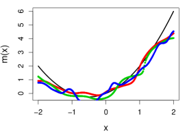
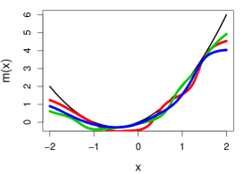
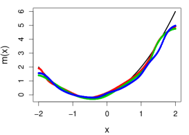
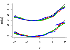
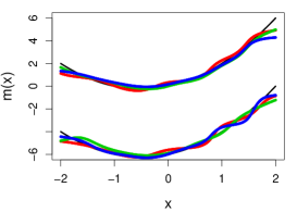
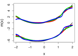
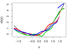
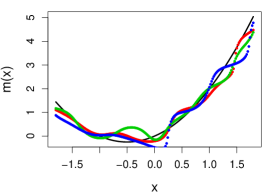
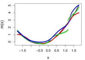
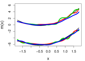
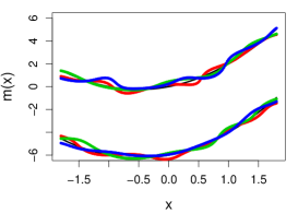
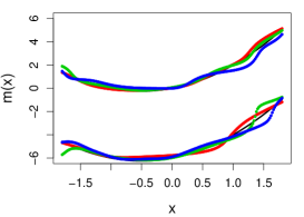
Table 1 shows the MC average of ISE of each mode (set) estimate across 500 MC replicates and the associated standard error under each simulation setting, with and . In terms of both ISE and variability, our mode estimates, and , outperform the naive mode estimate, denoted by , in all six settings. And the improvement of our estimates over the naive estimate is more substantial when the error contamination is more severe (i.e., for smaller ). In addition, the local linear estimate performs much better than the local constant estimate under (C1), while the advantage of the former is less obvious under (C2). In fact, deteriorates, although still outperforms , faster than does as decreases. The boxplots of ISEs and several estimated mode curves from each method are given in Appendix H, which clearly show that there are more outliers for compared to . This comparison between the two proposed mode estimators indicates that the local linear estimator may be more suitable when is unimodal, and can be subject to more numerical instability when applying to data from a multimodal distribution. This is reminiscent of a remark in Einbeck and Tutz (2006), who recommended use the local linear mode estimator (in the absence of measurement error in their study) “only for the case of functional dependence, i.e. where the mode is unique.”
(C1) (C2) 0.75 0.85 0.95 0.75 0.85 0.95 1.50 (0.21) 1.05 (0.15) 0.64 (0.10) 1.52 (0.29) 0.81 (0.12) 0.34 (0.05) 1.15 (0.17) 0.88 (0.13) 0.62 (0.10) 0.91 (0.16) 0.57 (0.09) 0.30 (0.04) 0.43 (0.10) 0.32 (0.07) 0.22 (0.05) 0.93 (0.31) 0.51 (0.13) 0.21 (0.04)
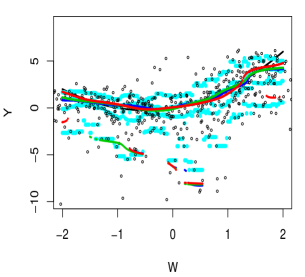
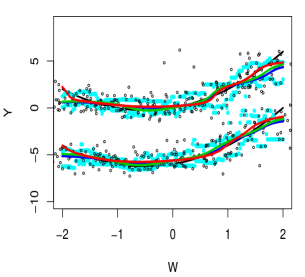
Acknowledging the fact that the approximated theoretical optimal is not available in practice, we carry out a second round of simulation under the same six settings, with fixed at for all three methods, used in our estimators chosen via the CV-SIMEX method with , and for the naive method chosen via naive CV as if were in (4.2). Table 2 shows the MC averages of ISE of the three considered estimates across 500 MC replicates, along with the corresponding standard errors, with . One can see that, under (C1), the proposed estimates still outperform the naive estimate. However, this is not as clear-cut under (C2). It appears that the number of modes in an estimated mode set (for any of these methods) can be sensitive to , and a smaller tends to give a bigger estimated mode set, creating more estimated local modes that can be far away from the true modes. As pictorial demonstration of these results, boxplots of these ISEs and several estimated mode curves from each method are provided in Appendix H.
(C1) (C2) 0.75 0.85 0.95 0.75 0.85 0.95 0.83 (0.19) 0.51 (0.12) 0.25 (0.06) 1.20 (0.51) 0.51 (0.11) 0.21 (0.03) 0.61 (0.15) 0.42 (0.11) 0.24 (0.05) 0.68 (0.37) 0.44 (0.39) 0.33 (0.40) 0.44 (0.12) 0.29 (0.08) 0.18 (0.07) 1.07 (0.54) 0.53 (0.29) 0.35 (0.60)
Besides the choice of , as pointed out in Section 5.1, the starting values for the mean-shift algorithm also affect finite sample performance of these estimators. We use the data-dependent starting values described in Section 5.1 in the first round of simulations where the approximated theoretical optimal is used. With the data-driven used in the estimates as in the second round of simulations, the quality of an estimate is even more sensitive to the choice of starting values. Figure 1 depicts the estimated mode curves from the three methods based on one simulated data set under each of (C1) and (C2), with the data-dependent starting values highlighted in turquoise. From there one can see that, if one starts at a starting mode value far away from the truth, the mean-shift algorithm can fail to converge or/and result in an inferior mode estimate. To avoid the interaction effects between the data-driven bandwidth selection and the data-dependent starting values, allowing us to focus on assessing the performance of the data-driven bandwidth selection, we set the starting values to be under (C1), and under (C2) when estimating in the second round of simulations that produce Table 2.
5.3 Dietary data
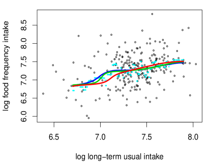
For illustration purposes, we consider estimating local modes of the food frequency questionnaire (FFQ) intake given one’s long-term usual intake using dietary data. The data set to be analyzed contains the FFQ intake, measured as percent calories from fat (), and six 24-hour food recalls from subjects in the Women’s Interview Survey of Health. The covariate of interest, the long-term usual intake (), cannot be observed directly. A common practice in epidemiology studies is to use data from 24-hour food recalls to construct a surrogate () of the true covariate. For instance, Liang and Wang (2005) used the average of two 24-hour food recalls from a subject as and studied the mean FFQ intake conditioning on and other error-free covariates; Wang et al. (2012) used the average of six 24-hour food recalls as and estimated conditional quantiles of the FFQ intake. All intake values are on the log scale in these studies. We followed the construction of in Wang et al. (2012), associated with which the estimated reliability ratio is 0.737.
Figure 2 presents the naive estimated mode curve and the two non-naive estimated mode curves from the two proposed methods. Both visual inspection of the scatter plot and the mean-shift algorithm seem to suggest a unimodal . Empirical evidence from simulation experiments suggest that this is the scenario where the local linear mode estimator can substantially improve over the naive estimator , and the local constant mode estimator can also correct to some extent. The discrepancy between the three estimated mode curves at the lower segments in Figure 2 can be due to bias correction from the two non-naive estimates, with the correction from more noticeable than that from .
6 Discussion
The study presented in this article fills in an important gap in the measurement error literature by providing mode estimation in the presence of measurement error. We rigorously study the asymptotic properties of the proposed mode estimators and develop a data-driven bandwidth selection method. This line of research leads us to more interesting open questions that we have started to investigate upon the completion of this project.
An immediate extension of this research is to allow the response prone to measurement error, with or without measurement error in covariates. An easy revision of the current estimator of the conditional (or joint) density is to replace with the corresponding deconvoluting kernel. The complication then, at least from the implementation standpoint, is that one will lose the mean-shift algorithm updating formula because the deconvoluting kernel for is no longer radially symmetric, the key feature of that leads to the updating formula in all existing mean-shift algorithm applications. A different mode seeking algorithm is needed in this case.
An even more involved problem arises from our development of data-driven bandwidth selection methods. In this study, we employed the CV-SIMEX method to select the bandwidth in the -direction, , with the bandwidth in the -direction, , fixed at the normal reference that only depends on the response data. We conjecture that a more sensible way to choose these two bandwidths is to choose them jointly according to some CV criterion tailored for mode estimation, as opposed to choosing them in two separate steps using two different CV criteria that are designed for density estimation. It is unclear at this point how to implement such joint selection while bearing in mind that and play very different roles, with one relating to an error-prone predictor and the other corresponding to an error-free response. Chen et al. (2016) assumed and then chose to minimize the volume of the estimated prediction set, a statistic constructed to strive for a balance between the number of estimated local modes and the distance between the estimated mode and . Following their idea, one may incorporate in the CV-SIMEX method the following CV criterion defined by (in the absence of measurement error)
where for a set , represents the estimated mode set at based on , is the number of distinct elements in , and is some weight function. However, theoretical justification of this CV criterion has not been established, and we did not see improvement from this bandwidth selection method over our current version of CV-SIMEX method in the simulation study (not shown here).
Besides the need for a new CV criterion for the purpose of mode estimation, we also believe that mode estimation, with or without measurement error, can benefit from using bandwidths that depend on . We gain this intuition from simulation study with multimodal , where we encountered more difficulty in estimating modes when multiple true mode curves are steeper and close to each other. This difficulty is expected and can be illustrated by Figure 3, where two pairs of curves are shown, with the left pair flat and the right pair steep (as functions of ). Fixing at an , the separation (in -direction) between two curves within each pair is the same in this figure, and the variability of around each mode curve is also the same. But, within a given window (of a fixed width) in the -direction, the data points (in red in Figure 3) surrounding the two steep curves are much harder to be separated into two clusters compared to the (red) data points around the two flat mode curves. And indeed in our simulation experiments (not shown here), the that works well for identifying the flat pair of mode curves does poorly in revealing the steep pair of the mode curves, and vice versa. Hence, if the multiple mode curves associated with show different steepness and different amount of separation along the -direction over different regions along the -direction, it seems more sensible to apply different bandwidths along .

In light of the need for variable bandwidths, the asymptotic optimal global bandwidths provided in Corollary 3.1 may seem irrelevant for the purpose of bandwidth selection, although they are theoretically valuable because they lead to optimal rates of MISE of the proposed mode estimators. Whether or not these optimal rates reach the minimax rate (given a well-defined class of mode estimators and a class of distributions or mode functions) remains an open problem. We conjecture that the key to solving this problem lies in the minimax convergence rate of MISE associated with nonparametric density derivative estimators in the presence of measurement error, which itself is an open problem that we will tackle next.
Appendix A: Technical conditions
Here we provide technical conditions that are needed at different parts of the theoretical development for different estimators considered in the main article.
(I) Conditions on the joint probability density
- (CP1)
-
The joint density is four times continuously differentiable with all partial derivatives bounded in absolute value by a finite positive constant .
- (CP2)
-
For where , there exists a finite positive constant such that .
Condition (CP1) is an ordinary smoothness condition. Condition (CP2) is a sharpness condition imposed on all critical points and implies no saddle points for .
(II) Conditions on kernels and
- (CK1)
-
is an even function and , for .
- (CK2)
-
is four times continuous differentiable with all derivatives bounded in absolute value, and , , for .
- (CK3)
-
and , for .
- (CK4)
-
, .
- (CK5)
-
, and .
- (CK6)
-
is supported on .
- (CK7)
-
is even and real.
- (CK8)
-
is not identically 0, for .
- (CK9)
-
The class of functions defined by
is a VC-type class (van der Varrt and Wellner, 1996), that is, there exist , , and a constant envelop such that , where is the -covering number for a semi-metric space and is any probability measure.
Define for . Then (CK1) implies that for all odd and , for . Condition (CK2) and (CK5) are needed to derive the uniform error rates of the proposed mode estimator. With , (CK3) gives equation (1.2) in Stefanski and Carroll (1990), the assumption necessary for a well-behaved deconvoluting kernel . Condition (CK3) with and (CK8) are needed to derive the mean and variance of . Conditions (CK4) and (the first half of) (CK5) are needed in Lemma B.4 in Delaigle et al. (2009), which we use to derive when is ordinary smooth. Conditions (CK4) and (CK6) are needed in Lemma B.9 in Delaigle et al. (2009), which we evoke to derive when is super smooth. Condition (CK7), along with (CU1) given later, are imposed so that is real. Finally, (CK9) is needed to obtain the uniform consistency of the kernel-based estimators involved in the study.
(III) Conditions on measurement error
- (CU1)
-
, , and it is an even function.
- (CU2)
-
.
Condition (CU1) is needed for a well-defined real-valued , for , and (CU2) is imposed in Lemma B.4 in Delaigle et al. (2009).
(IV) Conditions on the density of X, :
- (CX1)
-
, ; is twice differentiable and is bounded in absolute value by a finite positive constant , for .
This condition is needed for deriving the mean and variance of .
Appendix B: Relevant existing lemmas
In deriving we evoke Lemma B.4, Lemma B.6 (for ordinary smooth ) and Lemma B.9 (for super smooth ) in Delaigle et al. (2009). For completeness, these lemmas are restated next.
- Lemma B.4:
-
Assume that, for , , , , , and , then, for a bounded function ,
- Lemma B.9:
-
Suppose that is supported on , and, for and , . Then , where .
Appendix C: Asymptotic bias of
Assuming (CK3), it is shown that (Carroll and Hall, 1988; Stefanski and Carroll, 1990). Hence, , thus . We next focus on deriving .
Recall that
It follows that
| (C.1) | |||||
Under (CP1), has the third-order Taylor expansion around as follows,
| (C.2) |
where , , , and approach zero as , , , and other partial derivatives are similarly denoted. Given (CK1), using this third-order Taylor expansion in (C.1) leads to
which is equal to
when is the standard normal density, the choice we make in the main article. Hence,
| (C.3) |
Setting gives Lemma 3.1 in the main article.
Appendix D: Asymptotic variance of
Recall that
It follows that
| (D.1) |
From the bias analysis in Appendix C, we have
thus
| (D.2) |
This suggests that the second term in (D.1) is of order if , and it is of order if . We next look into the first term in (D.1).
With nondifferential measurement error, the joint pdf of is
| (D.3) |
It follows that
| (D.4) |
Using the first-order Taylor expansion of around in the innermost integral in (D.4) gives
where , for . Putting this elaboration of the innermost integral in (D.4) and using the first-order Taylor expansion of around in (D.4) gives
This reveals the dominating term of the expectation above as
| (D.5) |
When is ordinary smooth of order , by Lemma B.4 in Delaigle et al. (2009), which is repeated under Appendix B above, (D.5) indicates that
|
|
(D.6) |
where . Because (D.6) tends to zero slower than , (D.1) is dominated by the first term there. Hence, assuming , we have
Setting gives the first half of Lemma 3.2 in the main article, where is replaced by because is the standard normal pdf in the main article.
Appendix E: Convergence rate of
Assuming interchangeability of integrations, the mean integrated squared error (MISE) of can be decomposed into the sum of two parts,
By equation (17) in the main article, one has
| (E.1) | ||||
| (E.2) |
To derive the integrated squared bias, using (C.3) in (E.1), one has that, provided that tends to zero,
Under (CP2), and assuming and square integrable, one has
To derive the integrated variance, using the variance analysis Appendix D in (E.2), one has that, when is ordinary smooth,
and, when is super smooth,
Putting the above integrated squared bias of and integrated variance of together gives Theorem 3.2 in the main article.
Appendix F: Asymptotic bias of
F.1 Outline of deriving
Recall that . Denote by the first row of , then one has
| (F.1) |
The derivations of the dominating bias of involve two tasks. First, revealing the dominating terms in . Under (CX1), (CU1), and (CK1), (CK3)–(CK5), (CK8), Delaigle et al. (2009) showed that
where
Elaborating the above result yields
| (F.2) |
This completes the first task.
The second task is to reveal the dominating terms in according to the following decomposition,
| (F.3) |
Next, we first look into , then we study , and show that the former dominates that latter under certain conditions.
F.2 Deriving
Focusing on the case with , noting that and when is odd, for , (LABEL:eq:taylor) reduces to
| (F.7) |
F.3 Deriving
By (F.4), we have
| (F.8) | ||||
Next, we elaborate the two inner integrals, one w.r.t. and the other w.r.t. , in (LABEL:eq:twoinner).
For the inner integral w.r.t. , using the second-order Taylor expansion of around , one has
Setting , the above gives
| (F.10) | ||||
| (F.11) |
When it comes to the inner integral w.r.t in (LABEL:eq:twoinner), one shall distinguish between ordinary smooth and super smooth . If is ordinary smooth of order , under conditions (CK4) and (CK5), Lemma B.4 in Delaigle et al. (2009) implies that,
| (F.12) |
where , for . By (F.11) and (F.12), (LABEL:eq:twoinner) is equal to
| (F.13) | |||||
where “” is the convolution operator, that is, . Because the dominating term within the square brackets in (F.13) is
which is equal to by (D.3), (LABEL:eq:twoinner) indicates that, for ,
| (F.14) |
It follows that, when is ordinary smooth, the first term in (F.3) dominates the second term there if .
F.4 Concluding Lemma 3.3
Appendix G: Asymptotic variance of
By (F.2),
Extracting the dominating terms in the above expression reveals that, to find the dominating variance of , it suffices to look into the variance of
| (G.1) |
This leads us to study the following variance and covariance,
| (G.2) |
|
|
(G.3) |
G.1 Deriving the variance in (G.2)
For ,
| (G.5) | |||||
The expectation in (G.5) is considered in Section F.3 (see (F.8)). From there, we have shown that, if is ordinary smooth of order , then (relating to (F.14))
| (G.6) | |||||
and, if is super smooth of order , then (relating to (F.15))
| (G.7) | |||||
The expectation in (G.5) is considered in Section F.2 (see (F.2)). By (F.7), this expectation is of order when , and it is of order when . Hence, for both , (G.5) tends to zero faster than (G.6) and (G.7).
It follows that that, for ordinary smooth ,
| (G.8) | |||||
and, for super smooth ,
| (G.9) |
G.2 Deriving the covariance in (G.3)
G.3 Concluding Lemma 3.4
Appendix H: Pictorial demonstrations of simulation results












Appendix I: A sketch of the arguments in Section 3.1 with uni-modality assumption relaxed
Suppose has modes, with the mode set , and the estimated mode set . Then the pointwise error is . By the mean-value theorem, for each , one has
as in (3.2). It follows that
and thus
where the last equality results from assumption (CP2).
Hence, under the same conditions that supporting (3.3), can be approximated by , and thus the convergence rate of is the same as that of . From this point on, all arguments in Section 3 regarding , which is in Section 3.2 and is in Section 3.3, carry over to for each . And as long as is finite, the convergence rate of is the same as that of for a .
References
- Bamford et al. (2008) Bamford, S.P., Rojas, A.L., Genovese, C.R., Miller, C.E., and Nichol R, Wasserman, L. (2008) Revealing components of the galaxy population through nonparametric techniques. Mon. Not. R. Astron. Soc., 391, 607–616.
- Carroll and Hall (1988) Carroll, R. and Hall, P. (1988) Optimal rates of convergence for deconvoluting a density. J. Am. Statist. Ass., 83, 1184–1186.
- Carroll et al. (2006) Carroll, R., Ruppert, D., Stefanski, L. A. and Crainiceanu, C. M. (2006) Measurement error in nonlinear models: A model perspective. Second edition. Chapman & Hall/CRC. Boca Raton, FL.
- Chacón et al. (2011) Chacón, J. E., Duong, T. and Wand, M. P. (2011) Asymptotics for general multivariate kernel density derivative estimators. Stat. Sinica, 21, 807–840.
- Chen et al. (2015) Chen, Y., Genovese, C. R., Tibshirani, R. J. and Wasserman, L. (2015) Asymptotic theory for density ridges. Ann. Statist., 43, 1896–1928..
- Chen et al. (2016) Chen, Y., Genovese, C. R., Tibshirani, R. J. and Wasserman, L. (2016) Nonparametric modal regression. Ann. Statist., 44, 489–514.
- Cheng (1995) Cheng, Y. (1995) Mean shift, mode seeking, and clustering. IEEE. T. Pattern. Anal., 17, 790–799.
- Comaniciu and Meer (2002) Comaniciu, D. and Meer, P. (2002) Mean shift: a robust approach toward feature space analysis. IEEE. T. Pattern. Anal., 24, 603–619.
- Cook and Stefanski (1994) Cook, J. R. and Stefanski, L. A. (1994) Simulation-extrapolation estimation in parametic measurement error models. J. Am. Statist. Ass., 89, 1314–1328.
- Delaigle et al. (2009) Delaigle, A., Fan, J. and Carroll, R. (2009) A design-adaptive local polynomial estimator for the error-in-variables problem. J. Am. Statist. Ass., 104, 348–359.
- Delaigle and Hall (2008) Delaigle, A. and Hall, P. (2008) Using SIMEX for smoothing-parameter choice in errors-in-variables problems. J. Am. Statist. Ass., 103, 280-287.
- Delaigle et al. (2008) Delaigle, A., Hall, P. and Meister, A. (2008) On deconvolution with repeated measurements. Ann. Statist., 36, 665–687.
- Einmahl and Mason (2005) Einmahl, U. and Mason, D. M. (2005) Uniform in bandwidth consistency of kernel-type function estimators. Ann. Statist., 33, 1380–1403.
- Einbeck and Tutz (2006) Einbeck, J. and Tutz, G. (2006) Modelling beyond regression functions: an application of multimodal regression to space-flow data. J. R. Statist. Soc.B, 55, 461–475.
- Fan (1991a) Fan, J. (1991) Asymptotic normality for deconvolution kernel density estimators. Sankhya A, 53, 97–110.
- Fan (1991b) Fan, J. (1991) Global behavior of deconvolution kernel estimates. Stat. Sinica, 1, 541–551.
- Fan (1991c) Fan, J. (1991) On the optimal rates of convergence for nonparametric deconvolution problems. Ann. Statist., 19, 1257–1272.
- Fan and Gijbels (1996) Fan, J. and Gijbels, I. (1996) Local polynomial modelling and its applications, Chapman and Hall/CRC, Boca Raton.
- Fan and Truong (1993) Fan, J. and Truong, Y. K. (1993) Nonparametric regression with errors in variables. Ann. Statist., 21, 1900–1925.
- Fan et al. (1996) Fan, J., Yao, Q. and Tong, H. (1996) Estimation of conditional densities and sensitivity measures in nonlinear dynamical systems. Biometrika, 83, 189–206.
- Fan and Yim (2004) Fan, J. and Yim, T. H. (2004) A cross validation method for estimating conditional densities. Biometrika, 91, 819–834.
- Genovese et al. (2014) Genovese, C. R., Perone-Pacifico, M., Verdinelli, I., and Wasserman, L. (2014) Nonparametric ridge estimation. Ann. Statist., 42 1511–1545.
- Ginè and Guillou (2002) Ginè, E. and Guillou, A. (2002) Rates of strong uniform consistency for multivariate kernel density estimators. Ann. Inst. H. Poincarè Probab. Statist, 38 907–921.
- Hall et al. (2004) Hall, P., Racine, J., and Li, Q. (2004) Cross-validation and the estimation of conditional probability densities. J. Am. Statist. Ass., 99, 1015–1026.
- Hastie and Stuetzle (1989) Hastie, T. and Stuezle, S. (1989) Principal curves. J. Am. Statist. Ass., 44, 489–514.
- He and Liang (2000) He, X., and Liang, H. (2000) Quantile regression estimates for a class of linear and partially linear errors-in-variables models. Statist. Sin., 10, 129–140.
- Huang et al. (2013) Huang, M., Li, R., and Wang, S. (2013) Nonparametric mixture of regression models. J. Am. Statist. Ass., 108, 929–941.
- Hyndman et al. (1996) Hyndman, R. J., Bashtannyk, D. M. and Grunwald, G. K. (1996) Estimating and visualizing conditional densities. J. Comput. Graph. Stat., 5, 315–336.
- Koenker (2005) Koenker, R. (2005) Quantile regression. Cambridge University Press.
- Liang and Wang (2005) Liang, H. and Wang, N. (2005) Partially linear single-index measurement error models. Stat. Sinica, 15, 99–116.
- Ma and Yin (2011) Ma, Y. and Yin, G. (2011) Censored quantile regression with covariate measurement errors. Stat. Sinica, 21, 949–971.
- Nakamura (1990) Nakamura, T. (1990) Corrected score functions for errors-in-variables models: methodology and applications to generalized linear models. Biometrika, 77, 127–137.
- Novick and Stefanski (2002) Novick, S. J. and Stefanski, L. A. (2002) Corrected score estimation via complex variable simulation extrapolation. J. Am. Statist. Ass., 97, 472–481.
- Ozertem and Erdogmus (2011) Ozertem, U. and Erdogmus, D. (2011) Locally defined principal curves and surfaces. J. Mach. Learn. Res., 12, 1249–1286.
- Silverman (1986) Silverman, B.W. (1986) Density Estimation for Statistics and Data Analysis, Chapman and Hall.
- Stefanski and Carroll (1990) Stefanski, L. A. and Carroll, R. J. (1990) Deconvoluting kernel density estimators. Statistics, 21, 169–184.
- van der Varrt and Wellner (1996) van der Vaart, A. W. and Wellner, J. A. (1996) Weak convergence and empirical process: with applications to statistics. Springer, New York.
- Wand and Jones (1993) Wand, M. P. and Jones, M. C. (1993) Comparison of smoothing parameterizations in bivariate kernel density estimation. J. Am. Statist. Ass., 88, 520–528.
- Wang et al. (2012) Wang, H. J., Stefanski, L. A. and Zhu, Z. (2012) Corrected-loss estimation for quantile regression with covariate measurement errors. Biometrika, 99, 405-–421.
- Wei and Carroll (2009) Wei, Ying and Raymond, C. J. (2009) Quantile regression with measurement error. J. Am. Statist. Ass., 104, 1129–1143.
- Yao and Li (2014) Yao, W. and Li L. (2014) A new regression model: modal linear regression. Scand. J. Stat., 41, 656–671.
- Yao et al. (2012) Yao, W. and Lindsay, B. and Li, R. (2012) Local modal regression. J. Nonparametr. Stat., 24, 647–663.