Power Law of Shear Viscosity in Einstein-Maxwell-Dilaton-Axion model

Abstract

We construct charged black hole solutions with hyperscaling violation in the infrared(IR) region in Einstein-Maxwell-Dilaton-Axion theory and investigate the temperature behavior of the ratio of holographic shear viscosity to the entropy density. When translational symmetry breaking is relevant in the IR, the power law of the ratio is testified numerically at low temperature $T$, namely, $\eta/s\sim T^{\kappa}$, where the values of exponent $\kappa$ coincide with the analytical results. We also find that the exponent $\kappa$ is not affected by irrelevant current, but is reduced by the relevant current.

1.25.Tq, 04.70.Bw

1 Introduction

In last decade the development of holographic techniques has given new insights into the hydrodynamics with strong couplings. One celebrated achievement is the Kovtun-Son-Starinets (KSS) bound for the ratio of shear viscosity to entropy density [1]

$$\frac{\eta}{s}\geq\frac{1}{4\pi},$$ (1)

which is considered as a fundamental bound for near perfect fluid with strong interactions. However, in recent years counter-examples which violate the KSS bound (1) have been found in holographic literature, including the higher derivative gravity [2, 3], anisotropic system [6, 7, 4, 5] as well as isotropic system without translational invariance [9, 11, 12, 10, 8, 13, 14, 15]. In the latter case, shear viscosity loses its hydrodynamical interpretation because of the non-conservation of momentum and is usually defined by Kubo Formula

$$\eta=\lim_{\omega\to 0}\frac{1}{\omega}\text{Im}G^{R}_{\hat{T}^{xy}\hat{T}^{xy}}(\omega,k=0),$$ (2)

where $G^{R}_{\hat{T}^{xy}\hat{T}^{xy}}$ is the retarded Green function of the energy-momentum tensor operator $\hat{T}^{xy}$ in the dual boundary theory. Nevertheless, it is still quite instructive to investigate the temperature behavior of the ratio of shear viscosity to entropy density in general holographic models without translational invariance.

Historically, the breaking of translational invariance is introduced in holography to study the transportation of the dual system with momentum dissipation [18, 16, 17, 24, 23, 20, 19, 21, 22, 8, 25, 26, 27, 29, 30, 28]. In this setup, new geometries in the IR may emerge and often accompany with new scaling relations, leading to new scaling behavior of thermodynamic quantities or Green functions with temperature $T$ or frequency $\omega$ [37, 36, 35, 34, 33, 31, 38, 32, 39].

In particular, by virtue of recent progress in [9] people have learned that when the translation symmetry breaking is relevant in the far IR, the ratio exhibits a power law behavior with the temperature

$$\frac{\eta}{s}\sim T^{\kappa},$$ (3)

which reflects the scaling symmetry emerging in the IR. Moreover, a new bound for the exponent $\kappa$ was proposed as $\kappa\leq 2$ there, which might be supported by a heuristic argument based on the bound for the rate of entropy production,

$$\frac{\hbar}{k_{B}T}\frac{d\log(s)}{dt}\gtrsim 1.$$ (4)

Other holographic models are investigated in [14, 12, 11, 10, 8, 15], which also satisfy the bound $\kappa\leq 2$. But soon later in [13], we find $\kappa>2$ is possible when the scaling of Lifshitz [40, 41, 42] or hyperscaling violation [43, 44, 45, 46, 56, 47, 49, 50, 51, 52, 54, 55, 22, 48, 53, 57] emerges in the IR. While the bound for the rate of entropy production (4) is not violated, since the origin of the power law (3) should be understood as the nontrivial anomalous dimensions of (2) under the rescaling of the IR solution [9, 13].

Furthermore, in [13] we have analytically derived a formula for $\kappa$ in a general Einstein-Maxwell-Dilaton-Axion (EMD-Axion) model with spatial dimension $d$, dynamical critical exponent $z$ as well as hyperscaling violating exponent $\theta$. Specifically, we find

$$\frac{\eta}{s}\sim T^{\frac{d+z-\theta}{z}\left(-1+\sqrt{\frac{8(z-1)}{(d+z-\theta)(1+e^{2})}+1}\right)},$$ (5)

where $e^{2}$ is defined as the ratio of Maxwell term and one of the lattice terms in the Lagrangian. However, in [13] only for the case of $e^{2}=0$ has this formula (5) been justified by numerical calculation on neutral background. In this paper we intend to continuously testify the validity of (5) on charged background within EMD-Axion models. Schematically, the case of $e^{2}\neq 0$ can be realized by relevant currents. We will numerically construct specific charged backgrounds with ultraviolet(UV) completion and then compute the power law of the ratio of shear viscosity to entropy density. As a result, we will show that the formula for the ratio $\eta/s$ in (5) which was previously proposed in [13] based on the scaling analysis can be justified even for $e^{2}\neq 0$ indeed.

In this paper, we adopt the statement about ‘(marginally) relevant’ and ‘irrelevant’ in [32]: the current or the axion being (marginally) relevant means that the Maxwell or the axion terms is the same order as the curvature term and the dilaton potential in Lagrange in the power of the radial coordinate; the current or the axion being irrelevant means that the Maxwell or the axion terms is subleading comparing to the curvature term and the dilaton potential. Roughly speaking, a field being (marginally) relevant or irrelevant depends on whether or not it would deform the IR geometry strongly.

2 EMD-Axion model and hyperscaling violating metric

In this section we will present our holographic setup and then outline the logic leading to the formula for the exponent $\kappa$ in (5) based on the scaling analysis. The action of a general EMD-Axion model in $d+2$ space time reads as

$$\mathcal{S}=\int dtd^{d}xdr\sqrt{-g}(R+\mathcal{L}_{m}),\quad\mathcal{L}_{m}=-\frac{1}{2}(\partial\phi)^{2}-\frac{J(\phi)}{2}\sum_{i=1}^{d}(\partial\chi_{i})^{2}+V(\phi)-\frac{Z(\phi)}{4}F^{2},$$ (6)

where $\chi_{i}(i=1,2,\cdots,d)$ are axions and $J(\phi),Z(\phi),V(\phi)$ are coupling functions or potential of the dilaton field $\phi$. Given above action, the equations of motion can be derived as follows

$$R_{\mu\nu}+\frac{1}{d}{g_{\mu\nu}T}-T_{\mu\nu}=0,\quad T_{\mu\nu}=-\frac{1}{\sqrt{-g}}\frac{\delta(\sqrt{-g}\mathcal{L}_{m})}{\delta g^{\mu\nu}}=\frac{1}{2}g_{\mu\nu}\mathcal{L}_{m}-\frac{\delta\mathcal{L}_{m}}{\delta g^{\mu\nu}},$$ (7a)

$$\nabla^{2}\phi-\frac{J^{\prime}(\phi)}{2}\sum_{i=1}^{d}(\partial\chi_{i})^{2}+V^{\prime}(\phi)-\frac{Z^{\prime}(\phi)}{4}F^{2}=0,$$ (7b)

$$\nabla^{\nu}(Z(\phi)F_{\mu\nu})=0,$$ (7c)

$$\nabla^{\mu}(J(\phi)\partial_{\mu}\chi_{i})=0,\quad i=1,2,\cdots,d.$$ (7d)

For simplicity, we only consider isotropic solutions with following ansatz

$$\begin{split}&ds^{2}=-g_{tt}(r)dt^{2}+g_{rr}(r)dr^{2}+g_{xx}(r)\sum_{i=1}^{d}dx_{i}^{2},\\ &\phi=\phi(r),\quad\chi_{i}=kx_{i},\quad A=A_{t}(r)dt,\end{split}$$ (8)

where translational invariance is broken by the axions $\chi_{i}$ but the metric and energy-momentum tensor remain to be homogeneous.

As stated above, we are interested in solutions interpolating between AdS in the UV and hyperscaling violating solution in the IR. It can be realized by the process of UV completion [46]. Firstly, we construct a hyperscaling violation solution with running dilaton. Secondly, we modify the local behaviors of potentials to graft the solution onto AdS in the UV. Generally, solutions with AdS exist when the dilaton reaches the extremal point of its potential and the Lorentz symmetry is maintained [56].

Let us find hyperscaling violating solutions firstly. When the potentials behave as

$$V(\phi)\sim V_{0}e^{\alpha\phi},\quad J(\phi)\sim e^{\beta\phi},\quad Z(\phi)\sim e^{\gamma\phi},\quad\text{when }\phi\to\pm\infty,$$ (9)

it is found in [32, 31] that scaling solutions with hyperscaling violation exist, whose metric and matter fields read as

$$ds^{2}=r^{\frac{2\theta}{d}}\left(-\frac{dt^{2}}{r^{2z}}+\frac{L^{2}dr^{2}}{r^{2}}+\frac{\sum_{i=1}^{d}dx_{i}^{2}}{r^{2}}\right),\quad A=Qr^{\zeta-z}dt,\quad e^{\phi}=r^{\epsilon},\quad\chi_{i}=kx_{i},$$ (10)

where $k$ characterizes the scale of breaking of translational invariance and $\zeta$ is called conduction exponent [57]. Parameters $\{z,\theta,\zeta,\epsilon,k,Q\}$ in ansatz (10) are determined by equations of motion (7). The solutions are found to be classified into four classes [32], depending on the parameters $\{\alpha,\beta,\gamma,V_{0}\}$ in potentials (9). Among them, the explicit solutions with (marginally) relevant axion are shown in Appendix A. The metric in (10) can be deformed into a black hole solution

$$ds^{2}=r^{\frac{2\theta}{d}}\left(-\frac{f(r)dt^{2}}{r^{2z}}+\frac{L^{2}dr^{2}}{r^{2}f(r)}+\frac{\sum_{i=1}^{d}dx_{i}^{2}}{r^{2}}\right),$$ (11)

where the blackness function is

$$f(r)=1-\left(\frac{r}{r_{+}}\right)^{\delta_{0}},\quad\delta_{0}=d+z-\theta.$$ (12)

Then, the Hawking temperature and entropy density are separately given by

$$T=\frac{|\delta_{0}|}{4\pi}r_{+}^{-z},\quad s=4\pi r_{+}^{\theta-d}=4\pi\left(\frac{4\pi T}{|\delta_{0}|}\right)^{\frac{d-\theta}{z}}.$$ (13)

From Maxwell equation (7c), we have conserved charge density

$$\rho=\sqrt{-g}Z(\phi)F^{rt}.$$ (14)

It can be shown that there exists a scaling relation

$$x\to cx,\,r\to cr,\,t\to c^{z}t,\,ds\to c^{\theta/d}ds,\,T\to c^{-z}T,\,s\to c^{d-\theta}s.$$ (15)

We will come back to the UV completion and modify the potentials in next section.

Now we turn to the study of shear viscosity $\eta$. From Kubo formula (2), $\eta$ can be derived by perturbing $(\delta g)^{x}{}_{y}=g^{xx}\delta g_{xy}=h(r)e^{-i\omega t}$, which is the dual field of operator $\hat{T}^{xy}$. Einstein equations (7a) give rise to the shear perturbation equation

$$\frac{1}{\sqrt{-g}}\partial_{r}(\sqrt{-g}g^{rr}\partial_{r}h(r))+(g^{tt}\omega^{2}-m(r)^{2})h(r)=0,$$ (16)

with varying mass

$$m(r)^{2}=2(g^{xx}T_{xx}-\frac{\delta T_{xy}}{\delta g_{xy}}).$$ (17)

$h(r)$ is required to be regular at the horizon and equal to $1$ at the conformal boundary $r_{\partial}$. The varying mass is supposed to satisfy the condition $m(r)^{2}\geq 0$ in the models considered so far. Here, we have $m(r)^{2}=J(\phi)k^{2}g^{xx}$.

$\eta/s$ can be obtained by the weaker horizon formula [58, 9]

$$\frac{\eta}{s}=\frac{1}{4\pi}h_{0}(r_{+})^{2},$$ (18)

where $h_{0}(r)$ is the solution at $\omega=0$ and $r_{+}$ is the location of horizon.

Following the analysis presented in [13], one can calculate the exponent $\kappa$ of $\frac{\eta}{s}\sim T^{\kappa}$. Here we present a simpler derivation with the use of formula (18). If the axion is (marginally) relevant, by using Einstein equations (7a) and black hole metric (11), we have

$$m(r)^{2}=M^{2}r^{-\frac{2\theta}{d}},\quad M^{2}=\frac{2\delta_{0}(z-1)}{(1+e^{2})L^{2}},$$ (19)

where

$$e(r)^{2}=-\frac{Z(\phi)}{4}F^{2}\left/\left(\frac{1}{2}J(\phi)(\partial\chi_{x})^{2}\right)\right.\geq 0,\quad\chi_{x}=kx.$$ (20)

$e(r)^{2}$ is just the ratio of the Maxwell term to one of the axion terms in Lagrangian (6). It goes to a nonzero constant in the far IR if the current is also (marginally) relevant, otherwise it goes to zero. Thus at leading order, we just set $e(r)^{2}=e^{2}$. If the axion is irrelevant, $m(r)^{2}$ goes to zero in the far IR, then we set $M^{2}=0$, which is valid at leading order.

By using (19) and metric (11), we rewrite perturbation equation (16) at $\omega=0$

$$\partial_{r}(r^{1-\delta_{0}}f(r)\partial_{r}h_{0}(r))-M^{2}L^{2}r^{-\delta_{0}-1}h_{0}(r)=0.$$ (21)

Solving this equation we can separately obtain the asymptotical expansion of $h_{0}(r)$ near the boundary and its value on the horizon as

$$h_{0}(r\to r_{i})=c\left[\left(\frac{r}{r_{+}}\right)^{\delta_{0}-\delta_{\hat{T}}}+\cdots+G\left(\frac{r}{r_{+}}\right)^{\delta_{\hat{T}}}+\cdots\right],\quad h_{0}(r_{+})=cH,$$ (22)

where

$$\delta_{\hat{T}}=\frac{\delta_{0}}{2}\left(1+\sqrt{1+\left(\frac{2ML}{\delta_{0}}\right)^{2}}\right).$$ (23)

We have abbreviated the series $\left(\frac{r}{r_{+}}\right)^{\delta_{0}-\delta_{\hat{T}}+n\delta_{0}}$ ($n\geq 1$) following $\left(\frac{r}{r_{+}}\right)^{\delta_{0}-\delta_{\hat{T}}}$ and the series $\left(\frac{r}{r_{+}}\right)^{\delta_{\hat{T}}+m\delta_{0}}$ ($m\geq 1$) following $\left(\frac{r}{r_{+}}\right)^{\delta_{\hat{T}}}$ to ellipsis. $G$ and $H$ are some $r_{+}$ independent constants, which only depend on $\delta_{0}$ and $\delta_{\hat{T}}$. Coefficient $c$ should be determined by the boundary condition $h_{0}(r_{\partial})=1$. $r_{i}$ is the boundary of the region where the black hole with hyperscaling violation can be described by (11). When consider the second-order variation of the action in (6) over a fixed background with the perturbed metric $h_{0}(r)$, the boundary part of the variation with the branch of $r^{\delta_{0}-\delta_{\hat{T}}}$ ( $r^{\delta_{\hat{T}}}$) in (22) is divergent (finite), thus the branch of $r^{\delta_{0}-\delta_{\hat{T}}}$ ( $r^{\delta_{\hat{T}}}$) is non-normalizable (normalizable). Then $h_{0}(r_{i})\approx c\left(\frac{r_{i}}{r_{+}}\right)^{\delta_{0}-\delta_{\hat{T}}}$ is a good approximation when the black hole is near-extremal.

Since the UV completion is taken into account, one should be cautious that $r_{i}$ is just an intermediate scale but not the conformal boundary $r_{\partial}$. The region between $r_{i}$ and $r_{\partial}$ is AdS deformed by matter fields. The boundary condition requires $h_{0}(r_{\partial})=1$. As explained in [9], when going from $r_{\partial}$ to $r_{i}$, $h_{0}(r)$ decreases monotonously from 1 to a value $\Gamma$ when $m(r)^{2}>0$. We have introduced a ‘tunneling rate’ $\Gamma$ to characterize how $h_{0}(r)$ tunnels from $r_{\partial}$ to $r_{i}$. The tunneling rate $\Gamma$ and intermediate scale $r_{i}$ should be independent of $T$ when the scale of $T$ is much less than other scales, such as the source of dilaton and $k$ in axion. It is because that scale $T$ is not the dominating scale driving the renormalization group(RG) flow from AdS to hyperscaling violating solution. Scale $T$ becomes important only when we go into the far IR. Then we have

$$\Gamma=h_{0}(r_{i})\approx c\left(\frac{r_{i}}{r_{+}}\right)^{\delta_{0}-\delta_{\hat{T}}}.$$ (24)

By working out $c$, we can determine the horizon value

$$h_{0}(r_{+})=\Gamma H\left(\frac{r_{+}}{r_{i}}\right)^{\delta_{0}-\delta_{\hat{T}}}.$$ (25)

By virtue of formula (18), we finally obtain

$$\frac{\eta}{s}=\frac{\Gamma^{2}H^{2}}{4\pi}\left(\frac{r_{+}}{r_{i}}\right)^{2(\delta_{0}-\delta_{\hat{T}})}\propto T^{\frac{d-\theta+z}{z}\left(-1+\sqrt{1+\frac{8(z-1)}{(d-\theta+z)(1+e^{2})}}\right)},\text{ when }T\to 0,$$ (26)

where (13) and (23) have been used. One can also employ UV-IR matching [38, 59, 60] to reproduce the same result as what is performed in [13]. As one can see, when axion is absent or irrelevant, we have $m(r)^{2}=0$ at leading order, then $\eta/s\sim T^{0}$ [61, 62]. Next we will numerically testify this formula when $e^{2}=0$ or $e^{2}\neq 0$.

3 UV completion and numerical results

In this section we specifically construct the background interpolating hyperscaling violating solution (10) in the IR and AdS solution in the UV with finite temperature and charge density. On one hand, as explained in Appendix A or in [32], solution (10) can be constructed by choosing exponential potentials (9) with running dilaton. On the other hand, AdS can be constructed by finding extremal points of constant dilaton with lorentz symmetry. Here we adopt dilaton $\phi$ to interpolate the UV and the IR solutions. It requires some special settings for the potential $V(\phi)$.

3.1 UV completion

In this paper, we focus only on $\theta<d$ since in this region the entanglement entropy obeys area to volume law, which is considered as normal behavior of QFT [13, 53]. In this situation the location of IR is $r\to+\infty$. Following the discussion in [13, 56], the constraints about $(z,\theta)$ are reduced to

$$(\theta\leq 0\land z>1)\lor\left(0<\theta<d\land z>\frac{\theta}{d}+1\right).$$ (27)

Then it leads to $\delta_{0}>0$. We have excluded the two cases of $\theta=d$ and $z=\frac{\theta}{d}+1$ which can not be reached by running dilaton, as shown in Appendix (A) or [32]. We choose the branch of $\phi\geq 0$. From the requirement of the potentials (9), one can see that our solution can flow to hyperscaling violating solution in the IR if $\phi\to+\infty(r\to+\infty)$. It requires $\epsilon>0$ in (10). We conduct the UV completion by modifying the potential $V(\phi)$ but fixing the other two coupling potentials

$$J(\phi)=e^{\beta\phi},\quad Z(\phi)=e^{\gamma\phi}.$$ (28)

From the analysis in Appendix (A), we find a universal behavior of $V(\phi)\sim r^{-\frac{2\theta}{d}}$ in the coordinate of ansatz (10). So, when approaching the UV ($r\to 0$), the qualitative behavior of $V(\phi)$ depends on the sign of $\theta$. On the side of the UV, AdS is allowable if axion and gauge field are turned off and $\phi=\phi_{*}$ is an extremal point of $V(\phi)$, where $V(\phi_{*})$ stands for cosmological constant. Without loss of generality, we choose $\phi_{*}=0$. Then a realistic strategy is modifying $V(\phi)$ as

$$V(\phi)=\left\{\begin{array}[]{lll}\frac{2d}{\alpha^{2}}\sinh^{2}\left(\frac{\alpha\phi}{2}\right)+(d+1)d,&V_{0}=\frac{d}{2\alpha^{2}},&\text{ for }\theta<0\\ (d+1)d,&V_{0}=(d+1)d,&\text{ for }\theta=0\\ \left(d(d+1)-\frac{V_{0}}{2}\right)\left(1-\tanh^{2}(\alpha\phi)\right)+\frac{V_{0}}{2\cosh(\alpha\phi)},&V_{0}=2d\left(\frac{1}{\alpha^{2}}+2d+2\right),&\text{ for }d>\theta>0\end{array}\right..$$ (29)

In Appendix A, we have $\alpha\epsilon=-\frac{2\theta}{d}$. Then $\alpha$ has the opposite sign of $\theta$. So, as one can see, each $V(\phi)$ approaches $V_{0}e^{\alpha\phi}$ when $\phi\to+\infty$ and approaches $d(d+1)$ when $\phi\to 0$. Without loss of generality, we have chosen the AdS radius to be 1. However, the intermediate behavior is not very important.

$AdS_{d+2}$ vacuum is always allowable. We choose the first type quantization, and the scaling dimensions about the dual source of dilaton $\phi^{(0)}$ and operator $\mathcal{O}_{\phi}$ are determined by the small $\phi$ expansion of $V(\phi)$. When $\theta=0$, as dilaton is massless, we have $\Delta_{\phi^{(0)}}=0$ and $\Delta_{\mathcal{O}_{\phi}}=d+1$, which is marginal deformation. We expect it to be marginally relevant to drive the solution away from AdS, as $\phi=0$ is not a stable point when axion and gauge field are turned on. When $\theta\neq 0$, as $V(\phi)=d(d+1)+\frac{d}{2}\phi^{2}+\cdots$, we have $\Delta_{\phi^{(0)}}=1$ and $\Delta_{\mathcal{O}_{\phi}}=d$, which is relevant deformation.

3.2 Numerical calculation and results

We use the following ansatz for numerical calculation

$$\begin{split}&ds^{2}=\frac{1}{u^{2}}\left(-(1-u)U(u)e^{-S(u)}dt^{2}+\frac{du^{2}}{(1-u)U(u)}+\sum_{i=1}^{d}dx_{i}^{2}\right),\\ &\phi=\phi(u),\quad\chi_{i}=kx_{i},\quad A=(1-u)A(u)dt.\end{split}$$ (30)

The conformal boundary is located at $u=0$ while the horizon at $u=1$. The temperature and the entropy density are $T=\frac{1}{4\pi}U(1)e^{-S(1)/2}$ and $s=4\pi$.

The $AdS_{d+2}$ vacuum corresponds to $U=1,~{}S=\phi=A=0$. Boundary conditions at the horizon are regular conditions. Boundary conditions at conformal boundary should satisfy the scaling dimensions, which depend on the potential $V(\phi)$ as well as the value of $\theta$.

Explicitly, the asymptotic expansions near the conformal boundary are

$$\begin{split}U(u)&=1+\cdots+\varepsilon u^{d+1}+\cdots,\\ e^{-S(u)}&=1+\cdots,\\ A(u)&=\mu+\cdots+\rho u^{d-1}+\cdots,\\ \phi(u)&=\begin{cases}\lambda+\cdots+\nu u^{d+1}+\cdots,&\theta=0\cr\lambda u+\cdots+\nu u^{d}+\cdots,&\theta\neq 0\end{cases}\end{split}$$ (31)

where $\mu$ is the chemical potential and $e^{-S(0)}$ has been set to $1$ by rescaling $t$. The different boundary conditions of $\phi(u)$ come from the different choices of $V(\phi)$ in (29). We can work on either grand canonical ensemble or canonical ensemble.

3.2.1 Grand canonical ensemble

In grand canonical ensemble, we control the value of chemical potential $\mu$.

When $\theta=0$, the boundary conditions at conformal boundary are $U(0)=1,~{}S(0)=0,~{}A(0)=\mu,~{}\phi(0)=\lambda$. We work in the unit of $k$. The dimensionless quantities parameterizing the family of black hole solutions are $\{\frac{T}{k},~{}\frac{\mu}{k},~{}\lambda\}$. When $\theta\neq 0$, the boundary conditions are $U(0)=1,~{}S(0)=0,~{}A(0)=\mu,~{}\phi^{\prime}(0)=\lambda$. The dimensionless quantities are $\{\frac{T}{k},~{}\frac{\mu}{k},~{}\frac{\lambda}{k}\}$.

We numerically construct the interpolating solutions for $\phi\geq 0$. When dropping down $T/k$, we should fix the values of $\{\frac{\mu}{k},\lambda\}$ (for $\theta=0$) or $\{\frac{\mu}{k},\frac{\lambda}{k}\}$ (for $\theta\neq 0$) within an appropriate region respectively, in order to reach hyperscaling violating solution in the IR at low $T/k$.

The dimensionless entropy density and charge density are $s/k^{d}$ and $\rho/k^{d}$. We calculate $\eta/s$ by using (18) and found $\frac{\eta}{s}\leq\frac{1}{4\pi}$ for all the time, because of the breaking of translational invariance.

At high $T/k$, the scaling relation is controlled by AdS in the UV, which gives rise to the power laws of $s\sim T^{d}$ and $\frac{\eta}{s}\sim T^{0}$. On the other hand, at low $T/k$, the hyperscaling violation emerges in the IR. The power law of $s\sim T^{\frac{d-\theta}{z}}$ and $\frac{\eta}{s}\sim T^{\kappa}$ are observed in numerical results.

It is worthwhile to notice that $\rho/k^{d}$ converges to a nonzero constant at low $T/k$. When approaching the IR, $e^{2}(u)$ converges to a nonzero constant for class I but goes to zero as some power of radial coordinate $u$ for class II. Similarly, at low $T/k$, the horizon value $e^{2}_{h}=e^{2}(1)$ converges to a nonzero constant for class I but goes to zero as some power law for class II, whose exponent is shown in Appendix A. For the same $\{d,z,\theta\}$, it is observed that the appearance of a nonzero $e^{2}$ always reduces the exponent $\kappa$ of $\frac{\eta}{s}\sim T^{\kappa}$, which is consistent with the property that $\kappa$ decreases monotonously with $e^{2}$ in (26) when $\kappa>0$.

We conduct the numerical calculation for $d=2$ and $\theta=\frac{4}{3},~{}0,~{}-4$ as representives of three cases, namely $\theta<0,~{}\theta=0$ and $0<\theta<d$. Different values of $\gamma$ are chosen to represent class I or class II. The specific results are shown in Figure 1, 2, 3. All the numerical results match the analytical ones.

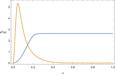
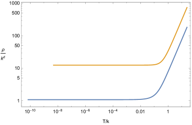
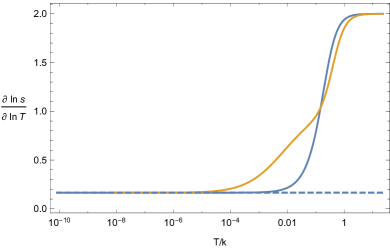
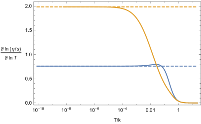
Figure 1: $d=2,~{}\theta=0$. Parameters are $\alpha=0,~{}\beta=-0.3$, $\gamma=0.6$ (blue) or $2$ (orange), then $z=12.1$. Among them, $\gamma=0.6$ belongs to class I; $\gamma=2$ belongs to class II. Solid lines denote numerical results and dashed lines denote analytical results from (13) and (26). Upper-left: Plot of $e^{2}(u)$ at rather low temperatures, where it converges to a nonzero constant in the IR for $\gamma=0.6$. Upper-right: Log-log plot of $\rho/k^{d}$ as a function of $T/k$, where $\rho/k^{d}$ converges to a constant at low temperature. Lower-left: Exponent $\lambda$ of $s\sim T^{\lambda}$ as a function of $T/k$. Lower-right: Exponent $\kappa$ of $\frac{\eta}{s}\sim T^{\kappa}$ as a function of $T/k$.

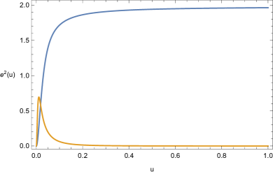
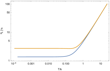
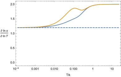
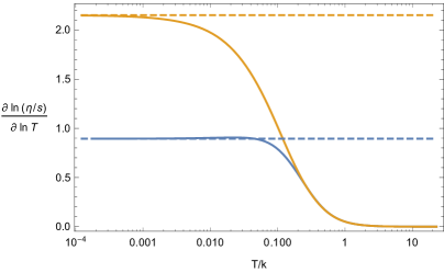
Figure 2: $d=2,~{}\theta<0$. Parameters are $\alpha=0.471,~{}\beta=-0.236$, $\gamma=0.943$ (blue, class I) or $2$ (orange, class II), then $z=5$ and $\theta=-4$.

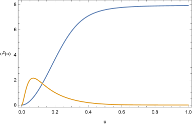
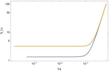
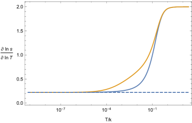
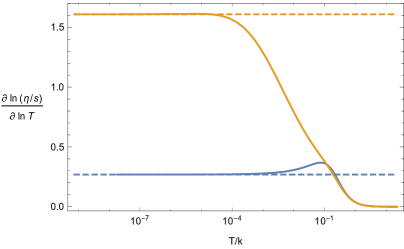
Figure 3: $d=2,~{}\theta>0$. Parameters are $\alpha=-1,~{}\beta=-1.5$, $\gamma=2$ (blue, class I) or $4$ (orange, class II), then $z=3$ and $\theta=1.33$.

3.2.2 Canonical ensemble

In canonical ensemble, we control the value of charge density $\rho$. The $t$ component of Maxwell equations (7c) can be replaced by (14).

When $\theta=0$, the three-parameter family of solutions is characterized by $\{\frac{T}{k},~{}\frac{\rho}{k^{d}},~{}\lambda\}$. When $\theta\neq 0$, the one is characterized by $\{\frac{T}{k},~{}\frac{\rho}{k^{d}},~{}\frac{\lambda}{k}\}$. When lowering down $T/k$, we fix the other two dimensionless parameters within an appropriate region. Then $\mu/k$ converges to a nonzero constant at low $T/k$ instead of $\rho/k^{d}$ in grand canonical ensemble. The behaviors of $\eta/s$ and $e^{2}$ are similar to those in grand canonical ensemble. By using the method in Appendix A, we can foresee the value to which $e^{2}$ converges in the IR at low temperature for class I.

In a parallel manner, we conduct the numerical calculation for $d=3$ and $\theta=-6,~{}0,~{}2$ to represent the three regions of $\theta<0,~{}\theta=0$ and $0<\theta<d$. The specific results are shown in Figure 4, 5 and 6. All the numerical results match the analytical ones.

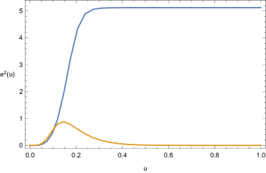
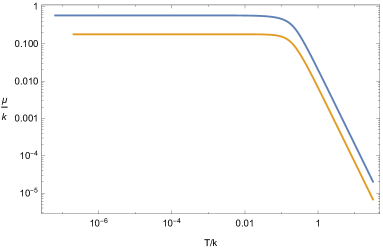
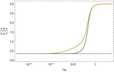
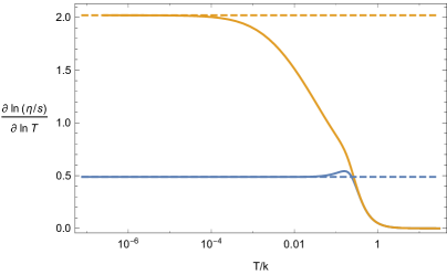
Figure 4: $d=3,~{}\theta=0$. Parameters are $\alpha=0,~{}\beta=-0.3$, $\gamma=0.9$ (blue, class I) or $2$ (orange, class II), then $z=8.41$. In the lower-right plot, it is worthwhile to notice that $\kappa$ converges to a quantity which is greater than $2$ at low temperature.

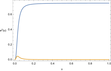
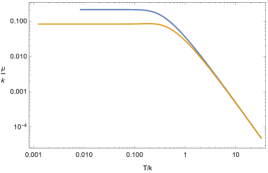
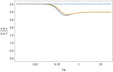
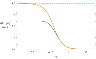
Figure 5: $d=3,~{}\theta<0$. Parameters are $\alpha=0.5,~{}\beta=-0.25$, $\gamma=1.75$ (blue, class I) or $3$ (orange, class II), then $z=2.56$ and $\theta=-6$.

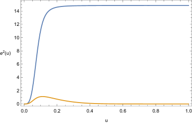
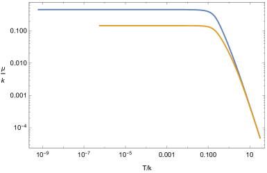
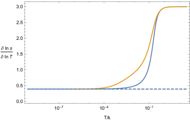
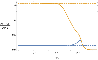
Figure 6: $d=3,~{}\theta>0$. Parameters are $\alpha=-1,~{}\beta=-1.5$, $\gamma=2.5$ (blue, class I) or $5$ (orange, class II), then $z=2.56$ and $\theta=2$.

4 Conclusion and Outlooks

In this paper we have numerically constructed charged solutions with emerging hyperscaling violation in EMD-Axion model and investigated the temperature behavior of the ratio of shear viscosity to entropy density. We have found that the relevant axion, which breaks the translational invariance, leads to the power law of $\eta/s\sim T^{\kappa}$. In particular, the relevant current reduces the exponent $\kappa$ indeed. This reduction is characterized by the quantity $e^{2}$, which can be derived from dimensionless conserved charge density $\rho/k^{d}$. While, irrelevant current does not affect the exponent $\kappa$ since $e^{2}\to 0$ in the far IR at low temperature. Our analytical results for the exponent $\kappa$ coincide with our numerical calculation, indicating that our proposed formula for $\kappa$ in (5) is robust at least for generic backgrounds within EMD-Axion model.

Especially, our results for Lifshitz case verify that $\kappa>2$ can happen in $d>2$, indicating that hyperscaling violation is not the essential ingredient leading to the exponent $\kappa>2$. Moreover, as conjectured in [13], the upper bounds for $\kappa$ coincide with the behaviors of entanglement entropy.

Analytically, it is possible that irrelevant current or axion can affect the temperature behavior of $\eta/s$ at subleading orders. One should consider their backreaction to the background, then solve the shear perturbation equation (16). It is related to the issue whether temperature $T$ is still the unique scale in entropy production, as it is when axion is relevant. It is worthy of investigation in the future.

Appendix A The classification of IR solutions

We focus on relevant axion solutions, otherwise $\eta/s$ just converges to a non-zero constant at low temperature at leading order. We require the solutions should have positive specific heat, and the temperature deformation is the only allowed relevant deformation. In addition, we give an extra requirement of $\theta<d$. The scaling solutions have been obtained and classified in [32, 31].

A.1 Class I: marginally relevant current, marginally relevant axion

If both the Maxwell and the axion terms are the same order in the power of the radial coordinate as the curvature term and the dilaton potential $V(\phi)$ in Lagrange (6), scaling solutions obtained form a one-parameter family

$$\begin{split}&\beta\epsilon=-2,\quad\alpha\epsilon=-\frac{2\theta}{d},\quad\gamma=\alpha(d-1)-\beta d,\quad\epsilon^{2}=\frac{2(d-\theta)(d(z-1)-\theta)}{d},\\ &\zeta=\theta-d,\quad L^{2}=\frac{2\left(\delta_{0}-1\right)\delta_{0}}{2V_{0}-(d-1)k^{2}},\quad Q^{2}=\frac{2\left(k^{2}(dz-\theta)+2V_{0}(1-z)\right)}{\delta_{0}\left((d-1)k^{2}-2V_{0}\right)},\end{split}$$ (32)

which can be parameterized by $k$ in coordinate of (10). The charge related quantities are

$$\rho^{2} = \frac{\delta_{0}^{2}Q^{2}}{L^{2}}=\frac{k^{2}(\theta-dz)+2V_{0}(z-1)}{\delta_{0}-1},$$ (33)

$$e^{2} = \frac{\delta_{0}^{2}Q^{2}}{L^{2}k^{2}}=\frac{k^{2}(\theta-dz)+2V_{0}(z-1)}{k^{2}(\delta_{0}-1)}.$$ (34)

The mode analysis in [32] indicates that there are three pairs of conjugate modes summing to $\delta_{0}$. Two pairs are degenerate with $\beta_{1,-}=\beta_{2,-}=0$ and $\beta_{1,+}=\beta_{2,+}=\delta_{0}$. $\beta_{1,-}$ rescales the time. $\beta_{1,+}$ is temperature deformation and responsible for creating a small black hole (11). $\beta_{2,-}$ changes $k$ and shifts the solution along the one-parameter family. $\beta_{2,+}$ changes the chemical potential and belongs to the transformation of gauge symmetry. The expression for the last pair of $\beta_{3,\pm}$ is too tedious to show here. We require that $\beta_{1,+}$ is relevant and $\beta_{3,-}$ is irrelevant, with IR located at $r\to\infty$. Then the final allowed parameter space here is found to be $\rho^{2}>0$ and (27).

Since the quantity $\frac{\rho}{k^{d}}=\frac{\sqrt{-g_{tt}g_{rr}g_{xx}^{d}}Z(\phi)F^{rt}}{(\partial_{x}\chi)^{d}}$ is conserved and invariant under coordinate transformation within (LABEL:metricandemtensor), we can use it to connect UV with IR and determine the solution in the one-parameter family by using (33). Finally, $e^{2}$ can be obtained from $\frac{\rho}{k^{d}}$ by using (34), which is rather convenient in canonical ensemble.

At zero temperature, one can integrate the three modes of $\beta_{2,-}$, $\beta_{2,+}$ and $\beta_{3,-}$ to the UV and adjust them to satisfy the boundary conditions specified by $\{\lambda,\rho,\mu\}$ at the conformal boundary. A finite temperature solution can be driven by $\beta_{1,+}$.

A.2 Class II: irrelevant current, marginally relevant axion

If only the Maxwell term turns to be subleading, a single scaling solution at leading order is obtained as

$$\begin{split}&\beta\epsilon=-2,\quad\alpha\epsilon=-\frac{2\theta}{d},\quad\epsilon^{2}=\frac{2(d-\theta)(d(z-1)-\theta)}{d},\\ &L^{2}=\frac{\delta_{0}(dz-\theta)}{V_{0}},\quad k^{2}=\frac{2V_{0}(z-1)}{dz-\theta}.\end{split}$$ (35)

There are three pairs of modes, in which two pairs sum to $\delta_{0}$. The first pair is $\beta_{1,-}=0$ and $\beta_{1,+}=\delta_{0}$ which are rescaling of time and temperature deformation. The second pair is relevant $\beta_{2,+}$ and irrelevant $\beta_{2,-}$. The third pair is gauge field modes with

$$A(r)=A_{1}+A_{2}r^{\zeta-z},\zeta=d-\theta+\frac{2\theta}{d}-\epsilon\gamma.$$ (36)

Mode of $A_{2}$ is irrelevant when $\delta_{0}(\zeta+d-\theta)<0$. We find $e^{2}(r)\sim r^{\zeta-d+\theta}$ and $\rho\sim T^{0},e^{2}_{h}\sim T^{\frac{\zeta-d+\theta}{-z}}$, when $T\to 0$. Similar to class I, we can integrate $\beta_{2,-}$ and gauge field modes to the UV.

References

- [1] P. Kovtun, D. T. Son and A. O. Starinets, Phys. Rev. Lett. 94: 111601 (2005)
- [2] M. Brigante, H. Liu, R. C. Myers et al, Phys. Rev. D 77: 126006 (2008)
- [3] Y. Kats and P. Petrov, JHEP 0901: 044 (2009)
- [4] D. Mateos and D. Trancanelli, Phys. Rev. Lett. 107: 101601 (2011)
- [5] D. Mateos and D. Trancanelli, JHEP 1107: 054 (2011)
- [6] A. Rebhan and D. Steineder, Phys. Rev. Lett. 108: 021601 (2012)
- [7] X. H. Ge, Y. Ling, C. Niu et al, Phys. Rev. D 92: no. 10, 106005 (2015)
- [8] R. A. Davison and B. Gout raux, JHEP 1501: 039 (2015)
- [9] S. A. Hartnoll, D. M. Ramirez and J. E. Santos, JHEP 1603: 170 (2016)
- [10] L. Alberte, M. Baggioli and O. Pujolas, arXiv:1601.03384 [hep-th].
- [11] P. Burikham and N. Poovuttikul, arXiv:1601.04624 [hep-th].
- [12] H. S. Liu, H. Lu and C. N. Pope, arXiv:1602.07712 [hep-th].
- [13] Y. Ling, Z. Y. Xian and Z. Zhou, arXiv:1605.03879 [hep-th].
- [14] Y. L. Wang and X. H. Ge, arXiv:1605.07248 [hep-th].
- [15] A. M. Garc a-Garc a, B. Loureiro and A. Romero-Berm dez, arXiv:1606.01142 [hep-th].
- [16] G. T. Horowitz, J. E. Santos and D. Tong, JHEP 1207: 168 (2012)
- [17] G. T. Horowitz and J. E. Santos, JHEP 1306: 087 (2013)
- [18] G. T. Horowitz, J. E. Santos and D. Tong, JHEP 1211: 102 (2012)
- [19] Y. Ling, C. Niu, J. P. Wu et al, JHEP 1311: 006 (2013)
- [20] S. A. Hartnoll and D. M. Hofman, Phys. Rev. Lett. 108: 241601 (2012)
- [21] M. Blake, D. Tong and D. Vegh, Phys. Rev. Lett. 112: no. 7, 071602 (2014)
- [22] E. Kiritsis and J. Ren, JHEP 1509: 168 (2015)
- [23] D. Vegh, arXiv:1301.0537 [hep-th].
- [24] T. Andrade and B. Withers, JHEP 1405: 101 (2014)
- [25] Y. Ling, P. Liu, C. Niu et al, JHEP 1502: 059 (2015)
- [26] M. Blake and A. Donos, Phys. Rev. Lett. 114: no. 2, 021601 (2015)
- [27] M. Baggioli and O. Pujolas, Phys. Rev. Lett. 114: no. 25, 251602 (2015)
- [28] R. A. Davison, K. Schalm and J. Zaanen, Phys. Rev. B 89: no. 24, 245116 (2014)
- [29] H. B. Zeng and J. P. Wu, Phys. Rev. D 90: no. 4, 046001 (2014)
- [30] A. Amoretti, A. Braggio, N. Maggiore et al, JHEP 1409: 160 (2014)
- [31] A. Donos and J. P. Gauntlett, JHEP 1406: 007 (2014)
- [32] B. Goutéraux, JHEP 1404: 181 (2014)
- [33] A. Donos, B. Goutéraux and E. Kiritsis, JHEP 1409: 038 (2014)
- [34] A. Donos and J. P. Gauntlett, JHEP 1404: 040 (2014)
- [35] S. A. Hartnoll and J. E. Santos, Phys. Rev. Lett. 112: 231601 (2014)
- [36] S. A. Hartnoll, D. M. Ramirez and J. E. Santos, JHEP 1509: 160 (2015)
- [37] S. A. Hartnoll, D. M. Ramirez and J. E. Santos, JHEP 1604: 022 (2016)
- [38] A. Donos and S. A. Hartnoll, Phys. Rev. D 86: 124046 (2012)
- [39] A. Donos and S. A. Hartnoll, Nature Phys. 9: 649 (2013)
- [40] S. Kachru, X. Liu and M. Mulligan, Phys. Rev. D 78: 106005 (2008)
- [41] M. Taylor, arXiv:0812.0530 [hep-th].
- [42] S. S. Gubser and A. Nellore, Phys. Rev. D 80: 105007 (2009)
- [43] S. S. Gubser and F. D. Rocha, Phys. Rev. D 81: 046001 (2010)
- [44] M. Cadoni, G. D’Appollonio and P. Pani, JHEP 1003: 100 (2010)
- [45] K. Goldstein, S. Kachru, S. Prakash et al, JHEP 1008: 078 (2010)
- [46] C. Charmousis, B. Goutéraux, B. S. Kim et al, JHEP 1011: 151 (2010)
- [47] E. Perlmutter, JHEP 1102: 013 (2011)
- [48] B. Goutéraux, J. Smolic, M. Smolic et al, JHEP 1201: 089 (2012)
- [49] B. Goutéraux and E. Kiritsis, JHEP 1112: 036 (2011)
- [50] N. Iizuka, N. Kundu, P. Narayan et al, JHEP 1201: 094 (2012)
- [51] N. Ogawa, T. Takayanagi and T. Ugajin, JHEP 1201: 125 (2012)
- [52] L. Huijse, S. Sachdev and B. Swingle, Phys. Rev. B 85: 035121 (2012)
- [53] X. Dong, S. Harrison, S. Kachru et al, JHEP 1206: 041 (2012)
- [54] M. Alishahiha and H. Yavartanoo, JHEP 1211: 034 (2012)
- [55] J. Bhattacharya, S. Cremonini and A. Sinkovics, JHEP 1302: 147 (2013)
- [56] B. Goutéraux and E. Kiritsis, JHEP 1304: 053 (2013)
- [57] B. Gout raux, JHEP 1401: 080 (2014)
- [58] A. Lucas, JHEP 1503: 071 (2015)
- [59] T. Faulkner, H. Liu, J. McGreevy et al, Phys. Rev. D 83: 125002 (2011)
- [60] T. Faulkner, N. Iqbal, H. Liu et al, Phil. Trans. Roy. Soc. A 369: 1640 (2011)
- [61] X. M. Kuang and J. P. Wu, arXiv:1511.03008 [hep-th].
- [62] K. S. Kolekar, D. Mukherjee and K. Narayan, arXiv:1604.05092 [hep-th].