Sparse Signal Subspace Decomposition Based on Adaptive Over-complete Dictionary

Abstract

This paper proposes a subspace decomposition method based on an over-complete dictionary in sparse representation, called ”Sparse Signal Subspace Decomposition” (or 3SD) method. This method makes use of a novel criterion based on the occurrence frequency of atoms of the dictionary over the data set. This criterion, well adapted to subspace-decomposition over a dependent basis set, adequately reflects the intrinsic characteristic of regularity of the signal. The 3SD method combines variance, sparsity and component frequency criteria into an unified framework. It takes benefits from using an over-complete dictionary which preserves details and from subspace decomposition which rejects strong noise. The 3SD method is very simple with a linear retrieval operation. It does not require any prior knowledge on distributions or parameters. When applied to image denoising, it demonstrates high performances both at preserving fine details and suppressing strong noise.

1 INTRODUCTION

Signal subspace methods (SSM) are efficient techniques to reduce dimensionality of data and to filter out noise [1]. The fundamental idea under SSM is to project the data on a basis made of two subspaces, one mostly containing the signal and the other the noise. The two subspaces are separated by a thresholding criterion associated with some measures of information.

The two most popular methods of signal subspace decomposition are wavelet shrinkage [2] and Principal Component Analysis (PCA) [3]. Both techniques have proved to be quite efficient. However, wavelet decomposition depending on signal statistics is not equally adapted to different data, and requires some knowledge on prior distributions or parameters of signals to efficiently choose the thresholds for shrinkage. A significant advantage of the PCA is its adaptability to data. The separation criterion is based on energy which may be seen as a limitation in some cases as illustrated in the next section.

In recent years, sparse coding has attracted significant interest in the field of signal denoising [4]. A sparse representation is a decomposition of a signal on a very small set of components of an over-complete basis (called dictionary) which is adapted to the processed data. A difficult aspect for signal subspace decomposition based on such a sparse representation is to define the most appropriate criterion to identify the principal components (called atoms) from the learned dictionary to build the principal subspace. The non-orthogonal property of the dictionary does not allow to use the energy criterion for this purpose, as done with PCA.

To solve this problem, we introduce a new criterion to measure the importance of atoms and propose a SSM under the criterion of the occurrence frequency of atoms. We thus make benefit both from the richness of over-complete dictionaries which preserves details of information and from signal subspace decomposition which rejects strong noise.

The remainder of this paper is organized as follows: Section 2 presents two related works to signal decomposition. Section 3 introduce the proposed sparse signal subspace decomposition based on adaptive over-complete dictionary. Some experimental results and analysis are presented in Section 4. Finally, we draw the conclusion in section 6.

2 Review of PCA and Sparse Coding Methods

We start with a brief description of two well-established approaches to signal decomposition that are relevant and related to the approach proposed in the next section.

2.1 PCA based Subspace Decomposition

The basic tool of SSM is principal component analysis (PCA). PCA makes use of an orthonormal basis to capture on a small set of vectors (the signal subspace) as much energy as possible from the observed data. The other basis vectors are expected to contain noise only and the signal projection on these vectors is rejected.

Consider a data set $\{\mathbf{x}_{m}\in\mathbb{R}^{N\times 1}\}_{m=1}^{M}$ grouped in a matrix form $\mathbf{X}$ of size $N\times M$: $\mathbf{X}=\{\mathbf{x}_{m}\}_{m=1}^{M}$. The PCA is based on singular value decomposition (SVD) with singular values $\sigma_{i}$ in descending order obtained from:

$$\mathbf{X}=\mathbf{U}\mathbf{A}=\mathbf{U}\mathbf{\Sigma}\mathbf{V}^{T}$$ (1)

where $\mathbf{U}$ and $\mathbf{V}$ are unitary matrices of size $N\times N$ and $M\times M$ respectively ($\mathbf{U}^{T}\mathbf{U}=\mathbf{I}_{N},\mathbf{V}^{T}\mathbf{V}=\mathbf{I}_{M}$) and $\mathbf{\Sigma}=\begin{bmatrix}diag\left[\sigma_{1},\cdots,\sigma_{r}\right],\mathbf{0}\\ \mathbf{0}\end{bmatrix}$ of size $N\times M$ with $\sigma_{1}\geq\sigma_{2}\geq\cdots\geq\sigma_{r}>0$, $\{\sigma_{i}\}_{i=1}^{r}$ are positive real known as the singular values of $\mathbf{X}$ with rank $r$ ($r\leq N$).

Equation (1) can be re-written in a vector form as:

$$\left[\mathbf{x}_{1}\quad\mathbf{x}_{2}\cdots\mathbf{x}_{m}\cdots\mathbf{x}_{M}\right]=\left[\mathbf{u}_{1}\quad\mathbf{u}_{2}\cdots\mathbf{u}_{n}\cdots\mathbf{u}_{N}\right].\left[\bm{\alpha}_{1}\quad\bm{\alpha}_{2}\cdots\bm{\alpha}_{m}\cdots\bm{\alpha}_{M}\right]$$ (2)

where $\mathbf{U}=\{\mathbf{u}_{n}\in\mathbb{R}^{N\times 1}\}_{n=1}^{N}$ and $\mathbf{A}=\{\bm{\alpha}_{m}\in\mathbb{R}^{N\times 1}\}_{m=1}^{M}$. Equation (2) means that the data set $\{\mathbf{x}_{m}\}_{m=1}^{M}$ is expressed on the orthonormal basis $\{\mathbf{u}_{n}\}_{n=1}^{N}$ as $\{\bm{\alpha}_{m}\}_{m=1}^{M}$.

In the SVD decomposition given in equation (1), the standard deviation $\sigma_{i}$ is used as the measurement for identifying the meaningful basis vector $\mathbf{u}_{i}$. PCA takes the first $P(P<r)$ components $\{\mathbf{u}_{n}\}_{n=1}^{P}$ to span the signal subspace, and the remainders $\{\mathbf{u}_{n}\}_{n=P+1}^{r}$ are considered in a noise subspace orthogonal to the signal subspace. Therefore, projection on the signal subspace will hopefully filter out noise and reveal hidden structures. The reconstructed signal $\hat{\mathbf{S}}_{PCA}$ of size $N\times M$ is obtained by projecting in the signal subspace as

$$\hat{\mathbf{S}}_{PCA}=\left[\mathbf{u}_{1}\cdots\mathbf{u}_{P}\quad\mathbf{0}_{P+1}\cdots\mathbf{0}_{N}\right].\left[\bm{\alpha}_{1}\quad\bm{\alpha}_{2}\cdots\bm{\alpha}_{m}\cdots\bm{\alpha}_{M}\right]$$ (3)

The underlying assumption is that information in the data set is almost completely contained in a small linear subspace of the overall space of possible data vectors, whereas additive noise is typically distributed through the larger space isotropically. PCA, using the standard deviation as a criterion, implies that the components of the signal of interest in the data set have a maximum variance and the other components are mainly due to the noise. However, in many practical cases, some components with low variances might actually be important because they carry information relative to the signal details. On the contrary, when dealing with noise with non-Gaussian statistics, it may happen that some noise components may actually have higher variances. At last, note that it is often difficult to provide a physical meaning to the orthonormal basis $\{\mathbf{u}_{i}\}_{i=1}^{r}$ of the SVD decomposition (equation 2) although they have a very clear definition in the mathematical sense as orthogonal, independent and normal. It is therefore difficult to impose known constraints on the signal features when they exist after the principal component decomposition.

2.2 Sparse Decomposition

Recent years have shown a growing interest in research on sparse decomposition of $M$ observations $\{\mathbf{x}_{m}\in\mathbb{R}^{N}\}_{m=1}^{M}$ based on a dictionary $\mathbf{D}=\{\mathbf{d}_{k}\}_{k=1}^{K}\in\mathbb{R}^{N\times K}$. When $K>N$, the dictionary is said over-complete. $\mathbf{d}_{k}\in\mathbb{R}^{N}$ is a basis vector, also called atom since they are not necessarily independent. By learning from data set $\{\mathbf{x}_{m}\}_{m=1}^{M}$, the sparse decomposition is the solution of equation (4) [4]:

$$\{\mathbf{D},\bm{\alpha}_{m}\}=\operatorname*{argmin}\limits_{\mathbf{D},{\bm{\alpha}_{m}}}\parallel{\bm{\alpha}_{m}}\parallel_{0}+\parallel\mathbf{D}{\bm{\alpha}}_{m}-\mathbf{x}_{m}\parallel^{2}_{2}\leq\varepsilon,\quad 1\leq m\leq M$$ (4)

where $\bm{\alpha}_{m}=\left[\alpha_{m}(1)\;\alpha_{m}(2)\;\dots\;\alpha_{m}({K})\right]^{T}\in\mathbb{R}^{K\times 1}$ is the sparse code of the observation $\mathbf{x}_{m}$. The allowed error tolerance $\varepsilon$ can be chosen according to the standard deviation of the noise. An estimate of the underlying signal $\{\mathbf{s}_{m}\}_{m=1}^{M}$ embedded in the observed data set $\{\mathbf{x}_{m}\}_{m=1}^{M}$ would be:

$$\left[\hat{\mathbf{s}}_{1}\quad\hat{\mathbf{s}}_{2}\cdots\hat{\mathbf{s}}_{m}\cdots\hat{\mathbf{s}_{M}}\right]=\left[\mathbf{d}_{1}\quad\mathbf{d}_{2}\cdots\mathbf{d}_{k}\cdots\mathbf{d}_{K}\right] .\left[\bm{\alpha}_{1}\quad\bm{\alpha}_{2}\cdots\bm{\alpha}_{m}\cdots\bm{\alpha}_{M}\right]$$ (5)

$$\mbox{or equivalently}\quad\hat{\mathbf{S}}=\mathbf{D}\mathbf{A}$$

where the matrix $\mathbf{A}$ of size $K\times M$ is composed of $M$ sparse column vectors $\bm{\alpha}_{m}$.

The first term on the right side of equation (4) is a sparsity-inducing regularization that constrains the solution with the fewest number of nonzero coefficients in each of sparse code vectors $\bm{\alpha}_{m}(1\leq m\leq M)$. The underlying assumption is that a meaningful signal could be represented by combining few atoms. This learned dictionary adapted to sparse signal descriptions has proved to be more effective in signal reconstruction and classification tasks than PCA method, which is demonstrated in the next section. The second term in equation (4) is the residual of the reconstruction, based on the mean-square reconstruction error estimate in the same way as in PCA method.

On the other hand, we note that the dictionary $\mathbf{D}$, a basis in sparse decomposition, is produced by learning noisy data set $\{\mathbf{x}_{m}\}_{m=1}^{M}$, so the basis vectors $\{\mathbf{d}_{k}\}_{k=1}^{K}$ should be decomposed into a principal subspace and a residual subspace. However, it is impossible to exploit an energy-constrained subspace since $\{\mathbf{d}_{k}\}_{k=1}^{K}$ are not necessarily orthogonal or independent.

3 The Proposed Sarse Signal Subspace Decomposition (3SD)

In this section, we introduce a novel criterion to the subspace decomposition over a learned dictionary and a corresponding index of significance of the atoms. Then we propose a signal sparse subspace decomposition (3SD) method under this new criterion.

3.1 Weight Vectors of Learned Atoms

At first, we intend to find out the weight of the atoms. In the sparse representation given in (5), coefficient matrix $\mathbf{A}$ is composed by $M$ sparse column vectors $\bm{\alpha}_{m}$, each $\bm{\alpha}_{m}$ representing the weight of the observation $\mathbf{x}_{m}$, a local parameter for the $m^{th}$ observation. Let us consider the row vectors $\{\bm{\beta}_{k}\}_{k=1}^{K}$ of coefficient matrix $\mathbf{A}$ :

$$\mathbf{A} =\left[\bm{\alpha}_{1}\;\bm{\alpha}_{2}\;\cdots\;\bm{\alpha}_{M}\right]$$ (6)

$$=\begin{bmatrix}\alpha_{1}(1)\quad\alpha_{2}(1)\quad\cdots\quad\alpha_{M}(1)\\ \alpha_{1}(2)\quad\alpha_{2}(2)\quad\cdots\quad\alpha_{M}(2)\\ \vdots\quad\quad\quad\vdots\quad\quad\ddots\quad\quad\vdots\\ \alpha_{1}(K)\quad\alpha_{2}(K)\quad\cdots\quad\alpha_{M}(K)\end{bmatrix}=\begin{bmatrix}\bm{\beta}_{1}\\ \bm{\beta}_{2}\\ \vdots\\ \bm{\beta}_{K}\end{bmatrix}$$

$$\mbox{where}\quad\bm{\beta}_{k}=\left[\alpha_{1}(k)\;\alpha_{2}(k)\;\dots\;\alpha_{M}(k)\right]\in\mathbb{R}^{1\times M}$$

Note that the row vector $\bm{\beta}_{k}$ is not necessarily sparse. Then equation (5) can be rewritten as:

$$\hat{\mathbf{S}} =\mathbf{D}\mathbf{A}$$ (7)

$$=\left[\mathbf{d}_{1}\cdots\mathbf{d}_{k}\cdots\mathbf{d}_{K}\right].\left[\bm{\beta}_{1}^{T}\cdots\bm{\beta}_{k}^{T}\cdots\bm{\beta}_{K}^{T}\right]^{T}$$

Equation (7) means that the row vector $\bm{\beta}_{k}$ is the weight of the atom $\mathbf{d}_{k}$, which is a global parameter over the data set $\mathbf{X}$. Denoting $\|\bm{\beta}_{k}\|_{0}$ the $\ell^{0}$ zero pseudo-norm of $\bm{\beta}_{k}$. $\|\bm{\beta}_{k}\|_{0}$ is the number of occurrences of atom $\mathbf{d}_{k}$ over the data set $\{\mathbf{x}_{m}\}_{m=1}^{M}$. We call it the frequency of the atom $\mathbf{d}_{k}$ denoted by $f_{k}$:

$$f_{k}\triangleq Frequency(\mathbf{d}_{k}|\mathbf{X})=\|\bm{\beta}_{k}\|_{0}$$ (8)

In the sparse decomposition, basis vectors $\{\mathbf{d}_{k}\}_{k=1}^{K}$ are prototypes of signal segments. That allows us to take them as a signal patterns. Thereupon, some important features of this signal pattern could be considered as a criterion to identify significant atoms. It is demonstrated [5] that $f_{k}$ is a good description of the signal texture. Intuitively, a signal pattern must occur in meaningful signals with higher frequency even with a lower energy. On the contrary, a noise pattern would hardly be reproduced in observed data even with a higher energy.

It is reasonable to take this frequency $f_{k}$ as a relevance criterion to decompose the over-complete dictionary into a principal signal subspace and a remained noise subspace. Here, we use the word ”subspace”, but in fact these two subspaces are not necessary independent.

3.2 Subspace Decomposition Based on Overcomplete Dictionary

Taking vectors $\{\bm{\beta}_{k}\}_{k=1}^{K}$, we calculate their $\ell^{0}$-norms $\{\|\bm{\beta}_{k}\|_{0}\}_{k=1}^{K}$ and rank them in descending order as follows. The index $k$ of vectors $\{\bm{\beta}_{k}\}_{k=1}^{K}$ are belonging to the set $\mathbf{C}=\{1,2,\cdots,k,\cdots,K\}$. A one-to-one index mapping function $\pi$ is defined as:

$$\quad\quad\quad\quad\pi(\mathbf{C}\rightarrow\mathbf{C}):k=\pi(\tilde{k}),\quad\quad k,\tilde{k}\in\mathbf{C}$$ (9)

$$s.t.\quad\|\bm{\beta}_{\pi(1)}\|_{0}\geq\|\bm{\beta}_{\pi(2)}\|_{0}\geq\cdots\geq\|\bm{\beta}_{\pi(\tilde{k})}\|_{0}\geq\cdots\geq\|\bm{\beta}_{\pi(K)}\|_{0}$$

By the permutation $\pi$ of the row index $k$ of matrix $\mathbf{A}=\left[\bm{\beta}_{1}^{T}\cdots\bm{\beta}_{k}^{T}\cdots\bm{\beta}_{K}^{T}\right]^{T}$, the reordered coefficient matrix $\tilde{\mathbf{A}}$ becomes

$$\tilde{\mathbf{A}} =\left[\bm{\beta}_{\pi(1)}^{T}\quad\bm{\beta}_{\pi(2)}^{T}\cdots\bm{\beta}_{\pi(k)}^{T}\cdots\bm{\beta}_{\pi(K)}^{T}\right]^{T}$$ (10)

With corresponding reordered dictionary $\tilde{\mathbf{D}}=\{\mathbf{d}_{\pi(k)}\}_{k=1}^{K}$, equation (7) can be written as:

$$\hat{\mathbf{S}} =\tilde{\mathbf{D}}\tilde{\mathbf{A}}$$ (11)

$$=\left[\mathbf{d}_{\pi(1)}\cdots\mathbf{d}_{\pi(k)}\cdots\mathbf{d}_{\pi(K)}\right].\left[\bm{\beta}_{\pi(1)}^{T}\cdots\bm{\beta}_{\pi(k)}^{T}\cdots\bm{\beta}_{\pi(K)}^{T}\right]^{T}$$

Then, the span of the first $P$ atoms can be taken as a principal subspace $\mathbf{D}_{P}^{(\mathbf{S})}$ and the remaining atoms span a noise subspace $\mathbf{D}_{K-P}^{(N)}$ as:

$$\mathbf{D}_{P}^{(\mathbf{S})}=span\{\mathbf{d}_{\pi{(1)}},\mathbf{d}_{\pi{(2)}},\cdots,\mathbf{d}_{\pi{(P)}}\}$$ (12)

$$\mathbf{D}_{K-P}^{(N)}=span\{\mathbf{d}_{\pi{(P+1)}},\mathbf{d}_{\pi{(P+2)}},\cdots,\mathbf{d}_{\pi{(K)}}\}$$

An estimate $\hat{\mathbf{S}}_{P}$ of the underlying signal $\mathbf{S}$ embedded in the observed data set $\mathbf{X}$ can be obtained on the principal subspace $\mathbf{D}_{P}^{(\mathbf{S})}$ simply by linear combination:

$$\hat{\mathbf{S}}_{P} =\mathbf{D}_{P}^{(\mathbf{S})}.\mathbf{A}_{P}^{(\mathbf{S})}$$ (13)

$$=\left[\mathbf{d}_{\pi(1)}\cdots\mathbf{d}_{\pi(k)}\cdots\mathbf{d}_{\pi(P)}\right].\left[{\bm{\beta}}_{\pi{(1)}}^{T}\cdots{\bm{\beta}}_{\pi{(k)}}^{T}\cdots{\bm{\beta}}_{\pi{(P)}}^{T}\right]$$

3.3 Threshold of Atom’s Frequency

Determining the number $P$ of atoms spanning the signal subspace $\mathbf{D}_{P}^{(\mathbf{S})}$ is always a hard topic especially for wide-band signals. Here, $P$ is the threshold of atom’s frequency $f_{k}$ to distinguish a signal subspace and a noise subspace. One of the advantages of 3SD is that this threshold $P$ can be easily chosen without any prior parameter.

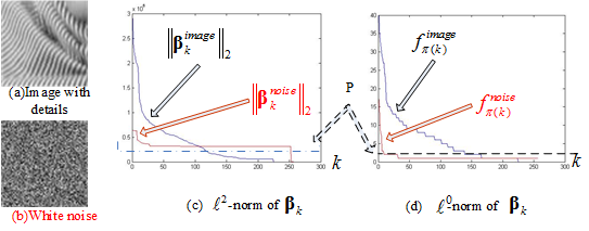
For a noiseless signal even with some week details, such as the image example in Fig. 1(a), the atoms’ frequencies $f_{\pi(k)}^{image}$s shown in Fig. 1(d) (in black line) are almost always high except the zero value. For a signal with strong noise, such as the example in Fig. 1(b), the atoms’ frequencies $f_{\pi(k)}^{noise}$s shown in Fig. 1(d) (in red line) are almost always equal to $1$ without zero and very few with value $2$ or $3$. It is easy to set a threshold $P$ of $f_{k}$ (dotted line in the Fig. 1(d)) to separate signal’s atoms from noise’s atoms. By contrast, the index numbers $\|\bm{\beta}_{k}\|_{2}$s under energy criterion shown in Fig. 1(c) for this example are rather puzzle to identify principal bases.

Figure 1: Sparse signal subspaces with criterion of atom’s frequency.

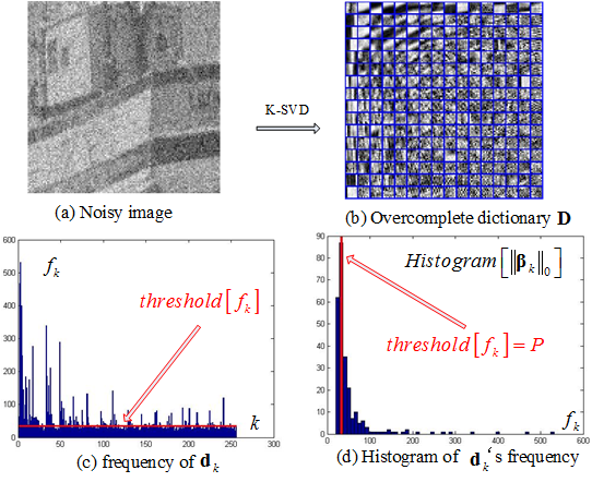
For a noisy signal, such as an image example in Fig. 2(a), its adaptive over-complete dictionary (Fig. 2(b)) consists of atoms of noiseless signal patterns, pure noise patterns and noisy signal patterns. Signal atoms should have higher frequencies, noise ones lower and noisy ones moderate. Intuitively, the red line (Fig. 2(c)) should be a suitable threshold $P$ of the frequencies $f_{k}$s. In practical implementation, the value of $P$ could be simply decided relying to the histogram of $f_{k}$. As shown in Fig. 2(d), one can set the value of $f_{k}$ associated to the maximum point of its histogram to $P$ as follows:

$$P=\operatorname*{arg\ max\ Hist}\limits_{k}{(\|\bm{\beta}_{k}\|_{0})}$$ (14)

Figure 2: The threshold $P$ of the frequencies $f_{k}$s.

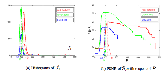
In fact, the performances in signal analyses by 3SD method are not sensitive to the threshold $P$, owed to the dependence of the atoms. To demonstrate this point, we take $3$ images, Barbara, Lena and Boat. Their histograms of $f_{k}$ are shown in Fig. 3(a) with the maximum points in dotted lines, $121$, $97$ and $92$ respectively. Fig. 3(b) reports the peak signal-to-noise ratio (PSNR) of the retrieved images $\hat{\mathbf{S}}_{P}$ on the signal principal subspace $\mathbf{D}_{P}^{(\mathbf{S})}$ with respect of $P$. We can see that PSNRs of the results remain the same in a large range around the maximum points (in dotted lines). Consequently, taking the value of $f_{k}$ associated to the maximum point of its histogram as the threshold $P$ is a reasonable solution.

Figure 3: The insensitivity of the threshold $P$.

4 Results and Discussion

4.1 Signal Decomposition Methods

Taking a part of the noisy Barbara image (Fig. 4(a)), we show an example of the sparse signal subspace decomposition (3SD) and the corresponding retrieved image (Fig. 4(b)). For comparison, the traditional sparse decomposition and the PCA based subspace decomposition are shown in Fig. 4(c) and Fig. 4(d).

Figure 4: Sparse signal decompositions and principal subspaces.

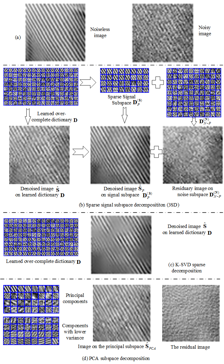
Let us look at the proposed sparse signal subspace decomposition on the top of Fig. 4(b) The $128$ atoms $\mathbf{d}_{k}$s of the learned overcomplete dictionary $\mathbf{D}$ are shown in descending order of their energies measured by $\|\bm{\beta}_{k}\|_{2}$. The $32$ principal signal atoms are chosen from the dictionary $\mathbf{D}$ under the frequency criterion. They are shown in descending order of their frequencies measured by $\|\bm{\beta}_{k}\|_{0}$ composing a signal subspace $\mathbf{D}_{32}^{(\mathbf{S})}$. We can see that some of the principal atoms are not among the first $32$ atoms with the largest energy in the overcomplete dictionary $\mathbf{D}$. The retrieved images are shown on the bottom of Fig. 4(b). The image $\mathbf{S}$ on $\mathbf{D}$ is apparently denoised. The image $\hat{\mathbf{S}}$ on the signal subspace $\mathbf{D}_{32}^{(\mathbf{S})}$ improves obviously by preserving fine details and at suppressing strong noise. On the other hand, the residual image on noise subspace $\mathbf{D}_{96}^{(N)}$ contains some very noisy information. This is because the atoms of the overcomplete dictionary are not independent.

For the same example, the classical sparse decomposition is shown in Fig. 4(c). Using K-SVD algorithm [6] in which the allowed error tolerance $\varepsilon$ (in equation (4)) is set to a smaller value to filter out noise. The retrieved image $\mathbf{S}$ seems to have a high Signal to Noise Ratio (SNR), but have lost the weak information. This is because signal distortion and residual noise cannot be minimized simultaneously at dictionary learning by equation (4).

In another comparison, the PCA based subspace decomposition is shown in Fig. 4(d). The $64$ components are orthonormal and the $32$ principal components are of the largest variance. The retrieved image by projecting on the signal subspace is rather noisy. This is because it cannot suppress strong noise and preserve weak details of information only using the variance criterion.

4.2 Application to Image Denoising

The application of 3SD to image denoising is presented here. A major difficulty of denoising is to separate underlying signal from noise. The proposed 3SD method could win this challenge. In 3SD method, the important components are selected from the over-complete dictionary relying to their occurrence number over the noisy image set. Evidently, the occurrence numbers would be large for signal, even for weak details, such as edges or textures and so on. On the other hand, the occurrence numbers would be low for different kinds of white Gaussian or non-Gaussian noises, even strong at intensity.

The 3SD algorithm for image denoising is presented as follows:

$\mathbf{Input}$:	Noisy image $\mathbf{X}$
$\mathbf{Output}$:	Denoised image $\hat{\mathbf{S}}$
-	Sparse representation $\{\mathbf{D},\mathbf{A}\}$: using K-SVD algorithm [6] by (4)
-	Identify principal atoms from $\mathbf{D}$ based on $\mathbf{A}$ :
	$\blacksquare$   Compute the frequencies of atoms $\{\|\bm{\beta}_{k}\|_{0}\}_{k=1}^{K}$ according to (6) and (8)
	$\blacksquare$   Get the permutation $\pi$ sorting the index $k$ of $\{\|\bm{\beta}_{k}\|_{0}\}_{k=1}^{K}$ by (9)
	$\blacksquare$   Compute the threshold $P$ by (14)
-	Obtain the signal principal atoms $\{\mathbf{d}_{\pi(k)}\}_{k=1}^{P}$ by (12)
-	Reconstruct image $\hat{\mathbf{S}_{P}}$ by (13)

In this application, we intend to preserve faint signal details under a situation of strong noise. We use the peak signal-to-noise ratio (PSNR) to assess the noise removal performance:

$$PSNR=20\cdot\log_{10}\left[MAX\{\mathbf{S}(i,j)\}\right]-10\cdot\log_{10}\left[MSE\right]$$ (15)

$$MSE=\frac{1}{IJ}{\sum\nolimits_{i=0}^{I-1}}{\sum\nolimits_{j=0}^{J-1}}\left[\mathbf{S}(i,j)-\hat{\mathbf{S}}(i,j)\right]^{2}$$

and the structural similarity index metric (SSIM) between the denoised image and the pure one to evaluate the preserving details performance:

$$SSIM(\mathbf{S},\hat{\mathbf{S}})=\frac{(2u_{\mathbf{S}}u_{\hat{{\mathbf{S}}}}+c_{1})(2\sigma_{\mathbf{S}\hat{{\mathbf{S}}}}+c_{2})}{(u^{2}_{\mathbf{S}}+u^{2}_{\hat{\mathbf{S}}}+c_{1})(\sigma^{2}_{\mathbf{S}}+\sigma^{2}_{\hat{\mathbf{S}}}+c_{2})}$$ (16)

where $u_{x}$ is the average of $x$, $\sigma_{x}^{2}$ is the variance of $x$, $\sigma_{xy}$ is the covariance of $x$ and $y$, and $c_{1}$ and $c_{2}$ are small variables to stabilize the division with weak denominator.

In the experiments, dictionaries used $D$s are of size $64\times 256$ ($K=256$ atoms), designed to handle image patches $\mathbf{x}_{m}$ of size $N=64=8\times 8$ pixels.

4.3 Image Denoising

A noisy Lena image $\mathbf{X}=\mathbf{S}+\mathbf{V}$ with an additive zero-mean white Gaussian noise $\mathbf{V}$ is used. The standard deviation of noise is $\sigma=35$. A comparison is made with 3SD method and K-SVD method [6] which is one of the best denoising methods reported in the recent literatures.

Figure 5: Image denoising comparing the proposed 3SD method with the K-SVD method.

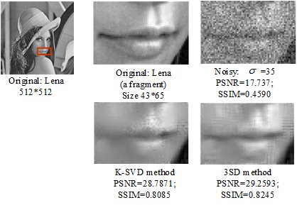
From the results shown in Fig. 5, the 3SD method outperforms the K-SVD method by about $1dB$ in PSNR and by about $1\%$ in SSIM (depending on how much details in images and how faint the details). In terms of subjective visual quality, we can see that the corner of mouth and the nasolabial fold with weak intensities are much better recovered by 3SD method.

4.4 SAR Image Despeckling

In the second experiment, a simulated SAR image with speckle noise is used. Speckle is often modeled as multiplicative noise as $x(i,j)=s(i,j)v(i,j)$ where $x$, $s$ and $v$ correspond to the contaminated intensity, the original intensity, and the noise level, respectively.

Figure 6: SAR image despeckling comparing the proposed 3SD method with the PPB method.

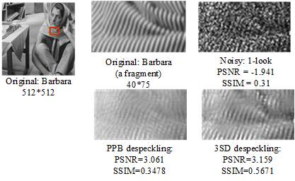
Fig. 6 shows the despeckling results of simulated one-look SAR scenario with a fragment of Barbara image. A comparison is made with 3SD method and a probabilistic patch based (PPB) filter based on nonlocal means approach [7] which can cope with non-Gaussian noise. We can see that PPB can well remove speckle noise. However, it also removes the low-intensity details. The 3SD method shows advantages at preserving fine details and at suppressing strong noise.

5 Conclusion

We proposed a method of sparse signal subspace decomposition (3SD). The central idea of the proposed 3SD is to identify principal atoms from an adaptive overcomplete dictionary relying the occurrence frequency of atoms over the data set (equation (8)). The atoms frequency is measured by zero pseudo-norms of weight vectors of atoms (equation (6) and (8)). The principal subspace is spanned by the maximum frequency atoms (equation (12)).

The 3SD method combines the variance criterion, the sparsity criterion and the component’s frequency criterion into a uniform framework. As a result, it can identify more effectively the principal atoms with the three important signal features. On the contrary, PCA uses only variance criterion and sparse coding method uses the variance and the sparsity criterions. In those ways, it is more difficult to distinguish weak information from strong noise.

Another interesting assert of 3SD method is that it takes benefits from using an over-complete dictionary which reserves details of information and from subspace decomposition which rejects strong noise. On the contrary, some undercomplete dictionary methods [8] and some sparse shrinkage methods [9, 10] might lose week information when suppressing noise.

Moreover, the 3SD method is very simple with a linear retrieval operation (equation (13)). It does not require any prior knowledge on distribution or parameter to determine a threshold (equation (14)). On the contrary, some sparse shrinkage methods, such as [9], necessitate non-linear processing with some prior distributions of signals.

The proposed 3SD could be interpreted as a PCA in sparse decomposition, so it admits straightforward extension to applications of feature extraction, inverse problems, or machine learning.

Competing interests

The authors declare that they have no competing interests.

Author’s contributions

HS proposed the idea, designed the algorithms and experiments, and drafted the manuscript. CWS gave suggestion on the design the algorithm, realized the algorithms, carried out the experiments. DLR gave suggestions on the mathematical expressions of munuscript and experiment analysis as well as explanation, and helped draft the manuscript.

References

- [1] Hermus, K., Wambacq, P., Hamme, H.V.: A review of signal subspace speech enhancement and its application to noise robust speech recognition. EURASIP Journal on Advances in Signal Processing, 888-896 (2007).doi:10.1155/2007/45821
- [2] Donoho, D.L., Johnstone, I.M., Kerkyacharian, G., Picard, D.: Wavelet shrinkage: asymptopia? Journal of the Royal Statistical Society. Series B 57, 301-369 (1995). http://citeseer.ist.psu.edu/viewdoc/summary?doi=10.1.1.162.1643
- [3] Tufts, D.W., Kumaresan, R., Kirsteins, I.: Data adaptive signal estimation by singular value decomposition of a data matrix. Proceeding of the IEEE 70(6), 684-685 (1982). doi:10.1109/PROC.1982.12367
- [4] Elad, M., Aharon, M.: Image denoising via sparse and redundant representations over learned dictionaries. IEEE Trans. Image Processing 15(12), 3736-3745 (2006). doi:10.1109/TIP.2006.881969
- [5] Variational texture synthesis with sparsity and spectrum constraints. Journal of Mathematical Imaging and Vision 52, 124-144 (2015). doi:10.1007/s10851-014-0547-7
- [6] Aharon, M., Elad, M., Bruckstein, A.: K-svd: an algorithm for designing overcomplete dictionaries for sparse representation. IEEE Trans. Signal Processing 54(11), 4311-4322 (2006). doi:10.1109/TSP.2006.881199
- [7] Deledalle, C.A., Denis, L., Tupin, F.: Iterative weighted maximum likelihood denoising with probabilistic patch-based weights. IEEE Trans. Image Processing 18(12), 2661-2672 (2009). doi:10.1109/TIP.2009.2029593
- [8] Porikli, F., Sundaresan, R., Suwa, K.: Sar depeckling by sparse reconstruction on affinity nets. EUSAR 2012 18,796-799 (2012).
- [9] Hyvarinen, A., Hoyer, P., Oja, E.: Sparse code shrinkage for image denoising. IEEE World Congress on Computational Intelligence 2, 859-864 (1998). doi:10.1109/IJCNN.1998.685880
- [10] Malutan, R., Terebes, R., Germain, C.: Speckle noise removal in ultrasound images using sparse code shrinkage.5th IEEE Conference on E-Health and Bioengineering Conference 2, 1-4 (2015).doi:10.1109/EHB.2015.7391394