Measuring the Breaking of Lepton Flavour Universality in $B\to K^{*}\ell^{+}\ell^{-}$

Abstract

We propose measurements of weighted differences of the angular observables in the rare decays $B\to K^{*}\ell^{+}\ell^{-}$. The proposed observables are very sensitive to the difference between the Wilson coefficients $\mathcal{C}_{9}^{(e)}$ and $\mathcal{C}_{9}^{(\mu)}$ for decays into electrons and muons, respectively. At the same time, the charm-induced hadronic contributions are kinematically suppressed to $\lesssim 7\%(4\%)$ in the region $1\,^{2}\leq q^{2}\leq 6\,^{2}$, as long as LFU breaking occurs only in $\mathcal{C}^{\text{$(\ell)$}}_{9}$. This suppression becomes stronger for the region of low hadronic recoil, $q^{2}\geq 15\,^{2}$.

I Introduction

In this letter, we investigate the suitability of new observables to measure the breaking of Lepton-Flavour Universality (LFU) in rare $b\to s\ell\ell$ transitions. While measurements Aaij et al. (2014); Wilson of the ratio $R_{K}$,

$$R_{K}\equiv\frac{\mathcal{B}(B\to K\mu^{+}\mu^{-})}{\mathcal{B}(B\to Ke^{+}e^{-})}\,,$$ (1)

for dilepton masses $1\,^{2}\leq q^{2}\leq 6\,^{2}$, hint toward LFU breaking, there has been no unambiguous discovery of such effects. It has been proposed Hiller and Schmaltz (2015) to expand such measurements to the decays $B\to X_{s}\ell^{+}\ell^{-}$, $B\to K^{*}\ell^{+}\ell^{-}$ and $B_{s}\to\phi\ell^{+}\ell^{-}$, introducing similar ratios $R_{X_{s}}$, $R_{K^{*}}$ and $R_{\phi}$, respectively. Analysing LFU breaking in angular observables of the decay $B\to K^{*}\ell^{+}\ell^{-}$ has been proposed in Altmannshofer and Straub (2015a), and more recently studied in Capdevila et al. (2016). Within this letter we propose observables that can be used to accurately measure the size of this breaking, specifically in the decays $B\to K^{*}\ell^{+}\ell^{-}$. Our study focuses on observables in which charm-induced long-distance contributions can be kinematically suppressed.

The exclusive decays $B\to K^{*}\ell^{+}\ell^{-}$ for $\ell=e,\mu$ are governed by the effective field theory for flavour-changing neutral $b\to s\{\gamma,\ell^{+}\ell^{-}\}$ transitions; see e.g. Bobeth et al. (2013). The theory’s Hamiltonian density to leading power in $G_{F}$ is

$${\cal{H}}^{(\ell)}_{\rm eff} =-\frac{4\,G_{F}}{\sqrt{2}}V_{tb}V_{ts}^{*}\,\Bigg{\{}\,\left[\frac{\alpha_{e}}{4\pi}\,\sum_{i}\mathcal{C}^{\text{$(\ell)$}}_{i}(\mu)\mathcal{O}_{i}^{(\ell)}\right]$$ (2)

$$+\left[\frac{e}{(4\pi)^{2}}\sum_{j}\mathcal{C}^{\text{}}_{j}(\mu)\mathcal{O}_{j}\right]+\left[\sum_{k}\mathcal{C}^{\text{}}_{k}(\mu)\mathcal{O}_{k}\right]$$

$$+\mathcal{O}\left({(V_{ub}V_{us}^{*})/(V_{tb}V_{ts}^{*})}\right)+\text{h.c.}\Bigg{\}}\,,$$

where $\mathcal{C}^{\text{}}_{i}(\mu)$ denotes the Wilson coefficients at the renormalisation scale $\mu$, and $\mathcal{O}_{\{i,j,k\}}$ denotes a basis of dimension-6 field operators. The index $i$ iterates over all semileptonic operators, $i=9,9^{\prime},10,10^{\prime},S,S^{\prime},P,P^{\prime},T,T5$, which are dependent on the final state lepton flavour $\ell=e,\mu$. The indices $j$ and $k$ iterate over the radiative ($j=7,7^{\prime}$), and the four-quark and chromomagnetic operators ($k=1,\dots,6,8$), respectively. The most relevant operators read

$$\mathcal{O}_{7(7^{\prime})} =\frac{m_{b}}{e}\!\left[\bar{s}\sigma^{\mu\nu}P_{R(L)}b\right]F_{\mu\nu}\,,$$ (3)

$$\mathcal{O}_{9(9^{\prime})} =\left[\bar{s}\gamma_{\mu}P_{L(R)}b\right]\!\left[\bar{\ell}\gamma^{\mu}\ell\right]\,,$$

$$\mathcal{O}_{10(10^{\prime})} =\left[\bar{s}\gamma_{\mu}P_{L(R)}b\right]\!\left[\bar{\ell}\gamma^{\mu}\gamma_{5}\ell\right]\,,$$

where a primed index indicates a flip of the quarks’ chiralities with respect to the unprimed, SM-like operator.

Hadronic matrix elements of the semileptonic operators are parametrized in terms of form factors, which can be determined using non-perturbative methods such as lattice QCD (see e.g. Horgan et al. (2014)) and QCD sum rules (see e.g. Bharucha et al. (2015)). However, hadronic matrix elements of the correlator between four-quark operators $\mathcal{O}_{i}\sim\left[\bar{s}\Gamma_{i}b\right]\,\left[\bar{q}\Gamma_{i}^{\prime}q\right]$, $i=1,\dots,6$ as well as the chromomagnetic operator $\mathcal{O}_{8}$ on the one hand, and the electromagnetic current on the other, are more complicated to estimate. These non-local matrix elements contribute to the transition amplitudes $A_{\lambda}$, with $\lambda=0,\perp,\parallel$, through shifts $\mathcal{C}^{\text{$(\ell)$}}_{9}\mapsto\mathcal{C}^{\text{$(\ell)$}}_{9}+h_{9,\lambda}(q^{2})$ and $\mathcal{C}^{\text{}}_{7}\mapsto\mathcal{C}^{\text{}}_{7}+h_{7,\lambda}$. Note that the shifts to $\mathcal{C}^{\text{}}_{9}$ are explicitly dependent on $q^{2}$, the momentum transfer to the lepton pair.

Within ratios of observables for either $\ell=\mu$ or $\ell=e$ final states, the non-local contributions $h_{9,\lambda}(q^{2})$ do not cancel completely. However, within differences of angular observables they can be kinematically suppressed.

The remainder of this letter is structured as follows: We propose the new observables in section II. Their numerical evaluations and theoretical uncertainties are discussed in section III. Thereafter, we study the experimental feasibility of their measurements for both future Belle-II and LHCb data sets in section IV, before we conclude in section V.

II Measures of LFU Breaking

The angular PDF for $B\to K^{*}(\to K\pi)\ell^{+}\ell^{-}$ decays is well known in the literature, and we use the conventions specified in Altmannshofer et al. (2009). There, the CP-averaged and normalized angular observables are

$$S_{i}(q^{2})\equiv\frac{4}{3}\,\frac{J_{i}(q^{2})+\overline{J}_{i}(q^{2})}{{\mathrm{d}}\Gamma\,/{\mathrm{d}}q\,^{2}+{\mathrm{d}}\overline{\Gamma}\,/{\mathrm{d}}q\,^{2}}\,,$$ (4)

where unbarred quantities stem from the decay $\bar{B}\to\bar{K}^{*}\ell^{+}\ell^{-}$, and the bar indicates CP conjugation. For the definitions of the $J_{i}$, see Kruger et al. (2000); Kruger and Matias (2005); Altmannshofer et al. (2009); Bobeth et al. (2013). Here and throughout the rest of this letter, we will refer to $S_{i}^{(\ell)}$ and $\Gamma^{(\ell)}$ as one of the angular observables or the decay width for the $\ell$ final state, respectively.

All spin-averaged observables can be expressed in terms of sesquilinear combinations of up to 14 transversity amplitudes when working in the full basis of dimension-six semileptonic operators Bobeth et al. (2013). For the discussions at hand, however, we restrict our study to the operators $\mathcal{O}_{9,10}$. In this case, all observables can be expressed in terms of only $7$ transversity amplitudes,

$$\frac{A_{0}^{L(R)}}{N\sqrt{\beta_{\ell}}} =-\left[\left(\mathcal{C}^{\text{eff,$(\ell)$}}_{9,0}\mp\mathcal{C}^{\text{}}_{10}\right)F_{V,0}\!+\!\frac{2m_{b}}{M_{B}}\mathcal{C}^{\text{eff}}_{7,0}F_{T,0}\!\right]$$ (5)

$$\frac{A_{\parallel}^{L(R)}}{N\sqrt{\beta_{\ell}}} =-\left[\left(\mathcal{C}^{\text{eff,$(\ell)$}}_{9,\parallel}\mp\mathcal{C}^{\text{}}_{10}\right)F_{V,\parallel}\!+\!\frac{2m_{b}M_{B}}{q^{2}}\mathcal{C}^{\text{eff}}_{7,\parallel}F_{T,\parallel}\!\right]$$

$$\frac{A_{\perp}^{L(R)}}{N\sqrt{\beta_{\ell}}} =\left[\left(\mathcal{C}^{\text{eff,$(\ell)$}}_{9,\perp}\mp\mathcal{C}^{\text{}}_{10}\right)F_{V,\perp}\!+\!\frac{2m_{b}M_{B}}{q^{2}}\mathcal{C}^{\text{eff}}_{7,\perp}F_{T,\perp}\!\right]$$

as well as $A_{t}$. The latter is not relevant to the discussions at hand. Note that our convention for the normalization constant $N$

$$N\equiv G_{F}\alpha_{e}V_{tb}V_{ts}^{*}\sqrt{\frac{q^{2}\sqrt{\lambda}}{3\cdot 2^{10}\pi^{5}M_{B}^{3}}}\,,$$ (6)

differs from, e.g., the normalization $N^{\text{\cite[cite]{\@@bibref{Authors Phrase1YearPhrase2}{Bobeth:2012vn}{\@@citephrase{(}}{\@@citephrase{)}}}}}$ as used in reference Bobeth et al. (2013): $N^{\text{\cite[cite]{\@@bibref{Authors Phrase1YearPhrase2}{Bobeth:2012vn}{\@@citephrase{(}}{\@@citephrase{)}}}}}=\sqrt{\beta_{\ell}}N$. Our choice ensures that the normalization is universal for all lepton flavours.

We propose to measure weighted differences of angular observables,

$$D_{i}(q^{2})\equiv\frac{{\mathrm{d}}\mathcal{B}^{(e)}\,}{{\mathrm{d}}q\,^{2}}S^{(e)}_{i}(q^{2})-\frac{{\mathrm{d}}\mathcal{B}^{(\mu)}\,}{{\mathrm{d}}q\,^{2}}S^{(\mu)}_{i}(q^{2})\,.$$ (7)

Assuming LFU breaking only in the Wilson coefficient $\mathcal{C}^{\text{}}_{9}$, we obtain for the indices $i=4,5,6s$ the expressions

$$\frac{-D_{4}(q^{2})}{\sqrt{2}\,N^{2}\,\tau_{B}} =\operatorname{Re}\left[\Delta_{9^{2}}^{(3)}\right]F_{V,\parallel}F_{V,0}$$ (8)

$$-\operatorname{Re}\left[\Delta_{9}^{(3)}\dots\right]+\mathcal{O}\left({\Delta_{\beta}^{(3)}}\right)\,,$$

$$\frac{D_{5}(q^{2})}{4\,\sqrt{2}\,N^{2}\,\tau_{B}} =\operatorname{Re}\left\{\Delta_{9}^{(2)}\mathcal{C}^{\text{}}_{10}\right\}F_{V,\perp}F_{V,0}$$

$$+\mathcal{O}\left({\Delta_{\beta}^{(2)}}\right)$$

$$\frac{D_{6s}(q^{2})}{8\,N^{2}\,\tau_{B}} =\operatorname{Re}\left\{\Delta_{9}^{(2)}\mathcal{C}^{\text{}}_{10}\right\}F_{V,\parallel}F_{V,\perp}$$

$$+\mathcal{O}\left({\Delta_{\beta}^{(2)}}\right)$$

where $\tau_{B}$ is the lifetime of the $B$ mesons, and the dots indicate an unsuppressed expression linear in the non-local contributions $h_{9,0}(q^{2})$ and $h_{9,\parallel}(q^{2})$. Moreover, we introduce

$$\Delta_{9^{l}}^{(k)} \equiv\beta_{e}^{k}\left[\mathcal{C}^{\text{$(e)$}}_{9}\right]^{l}-\beta_{\mu}^{k}\left[\mathcal{C}^{\text{$(\mu)$}}_{9}\right]^{l}\,,$$ (9)

$$\Delta_{\beta}^{(k)} \equiv\beta_{e}^{k}-\beta_{\mu}^{k}\,.$$

We find that eq. (8) holds up to corrections of order $\beta_{e}^{3}-\beta_{\mu}^{3}$ (for $D_{4}$) and $\beta_{e}^{2}-\beta_{\mu}^{2}$ (for $D_{5,6s}$). Note that $D_{4}$ is free of hadronic contributions in the term $\propto\Delta_{9^{2}}^{(3)}$, but not free of them in the linear term $\Delta_{9}^{(3)}$. For the full results, see eqs. (17)–(19). The expressions eq. (8) hold in the entire $q^{2}$ spectrum, since no explicit expression for the hadronic two-point correlation functions, $h_{9,\lambda}(q^{2})\equiv\mathcal{C}^{\text{eff,($\ell$)}}_{9,\lambda}(q^{2})-\mathcal{C}^{\text{$(\ell)$}}_{9}$, have been used. We emphasize that this also holds in between the two vetoes for the $J/\psi$ and $\psi(2S)$ charmonia.

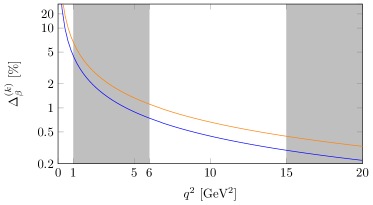
Figure 1: The $q^{2}$ dependence of the suppression terms $\Delta_{\beta}^{(k)}$ for $k=2$ (lower blue curve) and $k=3$ (upper orange curve), respectively, on a log scale. The windows in which either QCD-improved factorization or the operator product expansion at low recoil can be applied are indicated by the shaded area on the left and right, respectively.

For $q^{2}\geq 1\,^{2}$, the suppressed terms in eq. (8) scale with $\Delta_{\beta}^{(3)}<6.6\%$ and $\Delta_{\beta}^{(2)}<4.5\%$, respectively. For the low recoil region, these terms further shrink down to $<0.5\%$ and $<0.3\%$, respectively. Therefore, from a theoretical point of view, the low recoil region would be ideal for our proposed analysis. However, at LHCb the experimental analysis of the $e^{+}e^{-}$ final state is more challenging for large $q^{2}$.

While our approach is – in principal – also applicable to the angular observables $S_{i}$ with $i=7,8,9$, we remind that any observation of non-vanishing values for these observables already constitutes a sign of NP.

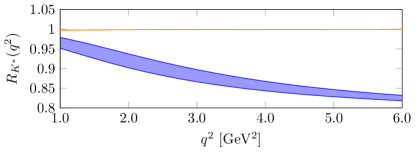
Figure 2: The $q^{2}$ behaviour of $R_{K^{*}}$ for our benchmark point $\mathcal{C}^{\text{$(e)$}}_{9}=\mathcal{C}^{\text{SM}}_{9}=\mathcal{C}^{\text{$(\mu)$}}_{9}+1$ (blue shaded area) and the SM (orange line). The illustrated uncertainty is due to our incomplete knowledge of the CKM matrix elements, the form factors, and the charm-induced long-distance contributions. The SM uncertainty too small to be shown.

Note that the proposed observables are not independent of $R_{K^{*}}$, the ratio of the decay rates into $\mu$ versus $e$, since:

$$D_{i}(q^{2}) =\left[\frac{{\mathrm{d}}\mathcal{B}^{(e)}\,}{{\mathrm{d}}q\,^{2}}+\frac{{\mathrm{d}}\mathcal{B}^{(e)}\,}{{\mathrm{d}}q\,^{2}}\right]$$ (10)

$$\times\left[\omega^{(e)}(q^{2})S^{(e)}_{i}(q^{2})-\omega^{(\mu)}(q^{2})S^{(\mu)}_{i}(q^{2})\right]\,,$$

with $\mathcal{B}^{(\ell)}$ the branching ratio of $B\to K^{*}\ell^{+}\ell^{-}$, and weights

$$\omega^{(e)}(q^{2}) \equiv\frac{1}{1+R_{K^{*}}(q^{2})}\,,$$ (11)

$$\omega^{(\mu)}(q^{2}) \equiv\frac{R_{K^{*}}(q^{2})}{1+R_{K^{*}}(q^{2})}\,.$$

Integration over $q^{2}$ from $a$ to $b$ then yields

$$\int_{a}^{b}{\mathrm{d}}q\,^{2}\,D_{i}(q^{2})\equiv\langle D_{i}\rangle_{a,b}\\ =\langle\mathcal{B}^{(e)}\rangle_{a,b}\,\langle S^{(e)}_{i}\rangle_{a,b}-\langle\mathcal{B}^{(\mu)}\rangle_{a,b}\,\langle S^{(\mu)}_{i}\rangle_{a,b}\,.$$ (12)

We also wish to comment on opportunities for decays other than $B\to K^{*}(\to K\pi)\ell^{+}\ell^{-}$:

1. The decays $B_{s}\to\phi(\to K^{+}K^{-})\ell^{+}\ell^{-}$, with $\ell=e,\mu$ can be described by the same angular PDF as $B\to K^{*}\ell^{+}\ell^{-}$ decays. Thus a generalization of the $D_{i}$ observables to the $B_{s}$ decay is obvious. However, measurements of the theoretically most interesting observables $S_{5,6s}$ will require flavour tagging. Notice that the feasibility for this measurement in LHCb is both limited by the observed yield in Run-I and the low tagging power capability. Moreover, a flavour-tagged analysis at Belle II is very difficult, since the production of $B_{s}$ pairs at the $\Upsilon(5S)$ resonance does not occur through eigenstates of the charge-conjugation operators (unlike production of $B_{d}$ pairs at the $\Upsilon(4S)$).

2. The observables $D_{i}$ can be generalized to the entire phase space of the $K\pi$ final state, i.e., to $K\pi$ masses outside the window that usually is associated with an on-shell $K^{*}(892)$. As for the $K^{*}(892)$, any significant deviation from zero, relative to the branching ratio, is a definite sign of LFU breaking, and thus a signal of NP. However, at the present time, the theoretical understanding of hadronic effects in $B\to K\pi\ell^{+}\ell^{-}$ is not well-enough developed for us to produce numerical estimates for small values of $q^{2}$.

3. The decays $\Lambda_{b}\to\Lambda(\to N\pi)\ell^{+}\ell^{-}$ give rise to 10 angular observables Böer et al. (2015). Amongst these observables, $K_{1c}$ and $K_{4s}$ permit a suppression of the charm-induced non-local matrix elements in the same fashion as shown in eq. (8). However, at the present time, measurements of the muon final state are affected by large statistical uncertainties, and no measurements for the electron final state are available.

III Numerical Results

In order to show that the observables $D_{4,5,6s}$ are indeed sensitive to LFU breaking, we evaluate them at large hadronic recoil in one bin $1\,^{2}\leq q^{2}\leq 6\,^{2}$, which we denoted as $\langle\cdot\rangle_{1,6}$. Our numerical calculations are carried out using the EOS software van Dyk et al. (2016a), which has been modified for this purpose van Dyk et al. (2016b). The evaluation of $B\to K^{*}\ell^{+}\ell^{-}$ observables in the large recoil region implements the results of the framework of QCD-improved factorization Beneke et al. (2001, 2005). The uncertainties on the $D_{i}$ arise dominantly from uncertainties of the CKM Wolfenstein parameters and our incomplete knowledge of the $B\to K^{*}$ form factors. The numerical input values, their sources and their prior PDFs are listed in table 1. In the SM, i.e., for $\mathcal{C}^{\text{$(e)$}}_{9}=\mathcal{C}^{\text{$(\mu)$}}_{9}=\mathcal{C}^{\text{SM}}_{9}$, we obtain

$$\langle R^{\text{SM}}_{K^{*}}\rangle_{1,6} =0.997^{+0.0005}_{-0.0004}\,,$$ (13)

$$\langle D^{\text{SM}}_{4}\rangle_{1,6} =(+2.9^{+1.1}_{-1.7})\cdot 10^{-10} (^{+39}_{-60}\%)\,,$$

$$\langle D^{\text{SM}}_{5}\rangle_{1,6} =(-1.1^{+2.0}_{-2.0})\cdot 10^{-10} (\pm 176\%)\,,$$

$$\langle D^{\text{SM}}_{6s}\rangle_{1,6} =(+4.4^{+1.7}_{-1.5})\cdot 10^{-10} (^{+40}_{-33}\%)\,.$$

The large relative uncertainties in the SM are to be expected, since for lepton-universal models the short-distance contributions on the right-hand side of eq. (8) are small compared to the correction that involve the hadronic contributions $h_{9,\lambda}$.

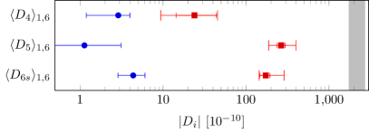
Figure 3: Comparison of the $q^{2}$-integrated observables $D_{i}$ in the SM (blue circles) with their values in the benchmark point (red squares) for the bin $1\,^{2}\leq q^{2}\leq 6\,^{2}$. The smaller (red) error marks correspond to the pure form factor uncertainties, while the larger (red) error marks correspond to the uncertainties as obtained for the data driven scenario; see the text for more information. The experimental measurement of branching ratio $\mathcal{B}(B\to K^{*}\mu^{+}\mu^{-})$, including the experimental uncertainty, is shown for comparison as the grey band.

However, in the case of LFU breaking, a sizeable leading short-distance term can reduce the relative size of he non-local hadronic uncertainties. For comparison, we define a benchmark point $\mathcal{C}^{\text{$(e)$}}_{9}=\mathcal{C}^{\text{SM}}_{9}=\mathcal{C}^{\text{$(\mu)$}}_{9}+1$. This point is favoured by several global analyses of data on $b\to s\ell^{+}\ell^{-}$ processes; see e.g. Beaujean et al. (2014); Altmannshofer and Straub (2015b); Descotes-Genon et al. (2016); Hurth et al. (2016). For our benchmark point (BMP) we obtain

$$\langle R^{\text{BMP}}_{K^{*}}\rangle_{1,6} =0.86^{+0.02}_{-0.01}\,,$$ (14)

$$\langle D^{\text{BMP}}_{4}\rangle_{1,6} =(+2.4^{+2.00}_{-0.95})\cdot 10^{-9} (^{+84}_{-40}\%)\,,$$

$$\langle D^{\text{BMP}}_{5}\rangle_{1,6} =(-2.7^{+0.31}_{-0.28})\cdot 10^{-8} (^{+12}_{-11}\%)\,,$$

$$\langle D^{\text{BMP}}_{6s}\rangle_{1,6} =(-1.7^{+0.21}_{-0.26})\cdot 10^{-8} (^{+12}_{-15}\%)\,,$$

where the uncertainties of $D_{5,6s}$ are now dominated by the parametric CKM and form factor uncertainties, while $D_{4}$ still shows large charm-induced uncertainties. A comparison between eq. (13) and eq. (14) clearly shows that the observables $D_{4,5,6s}$ are very sensitive to LFU-breaking NP effects, with relative enhancements (for the central values only) of

$$\frac{\langle D^{\text{BMP}}_{4}\rangle_{1,6}}{\langle D^{\text{SM}}_{4}\rangle_{1,6}} \simeq 8\,,$$ (15)

$$\frac{\langle D^{\text{BMP}}_{5}\rangle_{1,6}}{\langle D^{\text{SM}}_{5}\rangle_{1,6}} \simeq 200\,,$$

$$\frac{\langle D^{\text{BMP}}_{6s}\rangle_{1,6}}{\langle D^{\text{SM}}_{6s}\rangle_{1,6}} \simeq 40\,.$$

At the same time, it shows that the relative uncertainty is reduced slightly for $D_{4}$, and strongly for $D_{5,6s}$. This decrease in (relative) uncertainty emerges, since the impact of the non-local hadronic matrix elements is reduced compared to the now leading contributions from form factors and $\mathcal{C}^{\text{$(e)$}}_{9}-\mathcal{C}^{\text{$(\mu)$}}_{9}$.

Parameter	prior	unit	source
CKM Wolfenstein parameters
$\lambda$	$0.2253\pm 0.0006$	—	Bona et al. (2006)
$A$	$0.806\pm 0.020$	—	Bona et al. (2006)
$\bar{\rho}$	$0.132\pm 0.049$	—	Bona et al. (2006)
$\bar{\eta}$	$0.369\pm 0.050$	—	Bona et al. (2006)
Quark masses
$\overline{m}_{c}(\overline{m}_{c})$	$1.275\pm 0.025$		Olive et al. (2014)
$\overline{m}_{b}(\overline{m}_{b})$	$4.18\pm 0.03$		Olive et al. (2014)
$B\to K^{*}$ power correction parameters
$r_{0,\perp,\parallel}$	$1.00\pm 0.45$	—	this work

Table 1: Numerical inputs for the calculations of the electron and muons components of the observables $D_{i}$. The power corrections $r_{\chi}$, $\chi=0,\perp,\parallel$ are scaling factors to the dipole form factors $\cal{T}$ as introduced in Beneke et al. (2005). The prior distributions for all listed parameters are Gaussian, and the given intervals correspond to their central $68\%$ probability intervals. We do not list the $B\to K^{*}$ form factor parameters here, which are taken from a simultaneous fit to Light-Cone Sum Rule and lattice QCD results Bharucha et al. (2015), including their correlation matrix. For the data-driven scenario, we also use $B\to K$ form factor parameters as obtained in Khodjamirian et al. (2010).

We wish to further illustrate the usefulness of the newly-proposed observables by studying a data-driven scenario (DDS). For this, we carry out a Bayesian fit involving a free-floating $1.5\leq\mathcal{C}^{\text{$(\mu)$}}_{9}\leq 5.5$, while we fix all other Wilson coefficients to their SM values. The likelihood is comprised from the LHCb measurement of $R_{K}$ Aaij et al. (2014), a recent preliminary result for $R_{K}$ by the BaBar collaboration Wilson , as well as the LHCb results for $P^{\prime}_{5}$ Aaij et al. (2016), an angular observables in the decay $B\to K^{*}\mu^{+}\mu^{-}$ that exhibits reduced sensitivity to hadronic form factors. We then proceed to produce posterior-predictive distributions for $R_{K^{*}}$ and $D_{4,5,6s}$, which can be summarized as

$$\langle R^{\text{DDS}}_{K^{*}}\rangle_{1,6} =0.85\pm 0.04\,,$$ (16)

$$\langle D^{\text{DDS}}_{4}\rangle_{1,6} =(2.4^{+2.1}_{-1.5})\cdot 10^{-9}\,,$$

$$\langle D^{\text{DDS}}_{5}\rangle_{1,6} =(-3.1^{+0.9}_{-1.2})\cdot 10^{-8}\,,$$

$$\langle D^{\text{DDS}}_{6s}\rangle_{1,6} =(-2.1^{+0.8}_{-0.7})\cdot 10^{-8}\,,$$

which corresponds to qualitatively the same type of enhancements as in eq. (15). A comparison of all our numerical results for the $D_{4,5,6s}$ is depicted in figure 3.

IV Experimental Feasibility

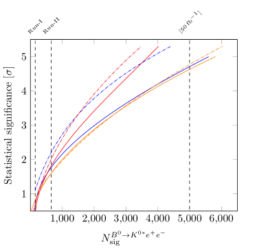
Figure 4: Projected statistical-only significance as a function of the extrapolated yields in LHCb for the (blue) $\langle D_{5}\rangle_{1,6}$ and (orange) $\langle D_{6s}\rangle_{1,6}$ observables, obtained from the (solid line) method-of-moments and (dash-dotted line) likelihood fit. The red lines indicate the combined significance of $\langle D_{5}\rangle_{1,6}$ and $\langle D_{6s}\rangle_{1,6}$.

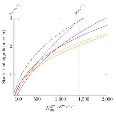
Figure 5: Projected statistical-only significance as a function of the extrapolated yields in Belle-II for the (blue) $\langle D_{5}\rangle_{1,6}$ and (orange) $\langle D_{6s}\rangle_{1,6}$ observables, obtained from the (solid line) method-of-moments and (dash-dotted line) likelihood fit. The red lines indicate the combined significance of $\langle D_{5}\rangle_{1,6}$ and $\langle D_{6s}\rangle_{1,6}$.

A series of signal-only ensembles of pseudoexperiments is generated to investigate the minimum amount of data required to claim an observation of NP in these observables. The simulation is performed without considering any experimental effects, i.e., background contributions, acceptance, resolution or bin migration. Similarly to the numerical calculations, the toy model is implemented using the EOS framework independently for each final state flavour at $1\,^{2}\leq q^{2}\leq 6\,^{2}$. Pseudoexperiments are generated with sample sizes corresponding roughly to the yields for the current and forthcoming data taking periods available at LHCb and Belle II.  These yields are extrapolated (rounded to the nearest 50/500) from the values reported in Aaij et al. (2014, 2016) and Abdesselam et al. (2016) by scaling the luminosities and the $b\bar{b}$ cross section $\sigma_{b\bar{b}}$. For LHCb, we scale $\sigma_{b\bar{b}}\propto\sqrt{s}$, while for Belle $\sigma_{b\bar{b}}\propto s$, where $s$ denotes the designed centre-of-mass energy of the $b$-quark pair. In particular, the significance for the range of $[3\,$-$\,50]\,$ and $[1\,$-$\,50]\,{\rm{ab}}^{-1}$ are examined for LHCb and Belle II, respectively. Note that the relative yields between electrons and muons are fixed in the pseudoexperiments. Ensembles with other sample sizes are also generated to test the scaling of the uncertainties, though only a representative subset of the results obtained are shown here.

A convenient strategy to determine the $S^{({\ell})}_{i}(q^{2})$, $\ell=e,\mu$ observables is to utilise the principal angular moments Beaujean et al. (2015). Although this approach provides an approximately $15\%$ worse precision on the measurement compared to the likelihood fit Aaij et al. (2016), as a proof-of-principle for the novel observables this is more robust (e.g. against mismodelling of the PDF) and insensitive to the choice of the estimated signal yield. Nevertheless, for completeness the results from an unbinned maximum likelihood fit are also reported. Note that the observables in both approaches correspond to the average $\langle S^{({\ell})}_{i}\rangle_{1,6}$, obtained by summing over each toy candidate for a given experiment.

Since the signal yield projections for the decay $B\to K^{*0}e^{+}e^{-}$ in both experiments indicate limited datasets, the stability of the likelihood fit is enforced by simplifying the differential decay rate. This is achieved by applying folding techniques to specific regions of the three-dimensional angular space, as detailed in Ref. Aaij et al. (2013). Notice that the angular analysis is performed separately for each lepton flavour. It is worth emphasizing that, despite potential benefits on the experimental side, to examine both final states simultaneously the choice to share/constrain angular observables across different flavours should be in general avoided – unless otherwise strongly motivated. For instance, assuming $\mathcal{C}^{\text{$(e)$}}_{9}=\mathcal{C}^{\text{SM}}_{9}=\mathcal{C}^{\text{$(\mu)$}}_{9}+1$, $F_{L}^{(\mu)}$ is reduced by $10\%$ compared to $F_{L}^{(e)}$.

Furthermore, it has been shown that an alternative approach to weighting each event by the inverse of its efficiency is given by the calculation of the unfolding matrix using the method of moments Beaujean et al. (2015). This is of particular interest in a simultaneous determination of the expressions $\omega^{(\ell)}(q^{2})$ (see eq. (11)) and $S^{(\ell)}_{i}(q^{2})$, in which a shared unfolded parametrisation can be used. Further advantages regarding the impact of common systematic effects are experiment dependent, and therefore, not discussed in this note.

In order to obtain the profile of the statistical-only significance for the extrapolated signal yields, both SM and NP simulated ensembles are examined. The resulting $\langle D_{i}\rangle_{1,6}$ observables are fitted, and the distance between the SM prediction and the fit results is calculated in units of the toy measurements’ standard deviations. Additional constraints on the likelihood fit were necessary in order to ensure the stability of the $\langle D_{6s}\rangle_{1,6}$ determination. In particular, the values of the longitudinal polarisation of the $K^{*0}$ meson and the transverse polarisation asymmetry are constrained within uncertainties to the theory predictions.

Figures 4 and 5 summarise the expected sensitivity to benchmark-like NP effects for the proposed observables $\langle D_{5}\rangle_{1,6}$ and $\langle D_{6s}\rangle_{1,6}$. Projections for $\langle D_{4}\rangle_{1,6}$ are not shown here since these are of limited usefulness. Further studies with realistic experimental effects are necessary to determine the exact sensitivities achievable. An extrapolation of the precision estimated here suggests that such measurements appear to be feasible, albeit that the confirmation of benchmark-like NP effects independently in each observable is only possible with the full capability of the experiments. Furthermore, the correlation between these observables can be estimated and used in a combined significance. Based on our extrapolations, a first evidence of NP in the LHCb measurement and considering only this novel approach can be achieved with $1300$ $B\to K^{*}e^{+}e^{-}$ signal events, which can currently not be expected to be recorded before the end of LHCb Run-II. Similar sensitivity in the Belle-II measurement can be achieved with $1500$ signal events, which corresponds roughly to an integrated luminosity of $50\,$ab^-1. Note that the possibility of the proposed approach to go beyond the usual theory upper bound of $q^{2}<6.0\,$GeV raises interesting prospects for Belle-II: first, to increase their sensitivity due to stronger suppression of the charm-induced contributions; and second, to record more events than currently considered.

V Conclusion

Recent measurements of $b\to s\ell^{+}\ell^{-}$ transitions show an interesting pattern of deviations with respect to SM predictions. In particular, the anomalous LHCb and Belle measurements of the observable $P_{5}^{\prime}$, and the LHCb measurement of the LFU-probing ratio $R_{K}$ can be simultaneously explained with NP contributions to the Wilson coefficients $\mathcal{C}^{\text{$(\mu)$}}_{9}$ and/or $\mathcal{C}^{\text{$(\mu)$}}_{10}$. This generated large attention in the flavour physics community, in particular concerning long-distance charm-induced effects, which might be able to explain the deviation in $P_{5}^{\prime}$.

Here, we proposed a new set of observables $D_{i}$ ($i=4,5,6s$), sensitive to LFU-breaking effects in the decays $B\to K^{*}\ell^{+}\ell^{-}$. These observables are branching-ratio-weighted averages of differences (with respect to the final-state lepton flavour) of the angular observables $S_{4,5,6s}$. In the presence of the LFU-breaking NP effects in $\mathcal{C}^{\text{$(\ell)$}}_{9}$, their theoretical uncertainties are dominated by $B\to K^{*}$ form factor and CKM parameter uncertainties, while non-local hadronic contributions are kinematically suppressed. This allows predictions in the NP scenarios that can be systematically improved as our knowledge of the $B\to K^{*}$ form factors and CKM Wolfenstein parameters improves. As examples we discussed here one benchmark point, as well as a data-driven scenario based on a fit of the observable $R_{K}$ and $P^{\prime}_{5}$. All these scenarios have peculiar patterns of deviations of the observables $D_{i}$ with respect to SM predictions (with reduced theoretical uncertainties). Therefore these new observables, in addition to providing sensitivity to discover NP with LFU-breaking effects, are useful to disentangle the different scenarios and are crucial to test the mutual consistency across different measurements. It is important to highlight that these observables are also independent of other LFU-breaking measurements, e.g. $R_{K}$ or $R_{\phi}$. Hence, these can be included in global fits, which improves the potential sensitivity to LFU-breaking NP effects.

The $D_{i}$ observables can be measured at the LHCb (and its upgrade) or at the Belle II experiments, either by performing likelihood fits of the angular distribution of the decays $B\to K^{*}\ell^{+}\ell^{-}$ or by using the method of moments. We found that in order to obtain $3\sigma$ evidence for NP in only these observables and using the method of moments, roughly 1500 $B\to K^{*}e^{+}e^{-}$ signal events are necessary in either experiment.

Our approach can be generalized for other decays to $K\pi\ell^{+}\ell^{-}$ final states. Here as well, a significant deviations from zero of the $D_{i}$ observables, relative in size to the branching ratio, would be a clear sign of NP. However the theoretical and experimental knowledge of the $K\pi$ invariant mass region outside the $K^{*0}(892)$ is not yet sufficient to provide solid numerical predictions.

Appendix A Additional Formulae

The full expressions for the observables $D_{4}$ through $D_{6s}$ in the basis of SM-like operators, assuming real valued Wilson coefficients and LFU-breaking only in the coefficient $\mathcal{C}^{\text{}}_{9}$, read:

$$\frac{-D_{4}(q^{2})}{\sqrt{2}\,N^{2}\,\tau_{B}} =\left[\Delta_{9^{2}}^{(3)}\right]F_{V,\parallel}F_{V,0}-\operatorname{Re}\left[\Delta_{9}^{(3)}(h_{9,\parallel}+h_{9,0})\right]F_{V,\parallel}F_{V,0}$$ (17)

$$-\frac{2m_{b}}{M_{B}}\operatorname{Re}\left[\Delta_{9}^{(3)}(\mathcal{C}^{\text{}}_{7}+h_{7,0})^{*}\right]F_{T,0}F_{V,\parallel}-\frac{2m_{b}M_{B}}{q^{2}}\operatorname{Re}\left[\Delta_{9}^{(3)}(\mathcal{C}^{\text{}}_{7}+h_{7,\parallel})^{*}\right]F_{T,\parallel}F_{V,0}$$

$$+\Delta_{\beta}^{(3)}\frac{2m_{b}^{2}}{s}\operatorname{Re}\left[(\mathcal{C}^{\text{}}_{7}+h_{7,0})(\mathcal{C}^{\text{}}_{7}+h_{7,\perp})^{*}\right]F_{T,0}F_{T,\parallel}$$

$$+\Delta_{\beta}^{(3)}\left\{\left|\mathcal{C}^{\text{}}_{10}\right|^{2}+\operatorname{Re}\left[h_{9,0}h^{*}_{9,\parallel}\right]\right\}F_{V,0}F_{V,\parallel}$$

$$+\Delta_{\beta}^{(3)}\frac{2m_{b}M_{B}}{q^{2}}\operatorname{Re}\left[(\mathcal{C}^{\text{}}_{7}+h_{7,\parallel})h^{*}_{9,0}\right]F_{T,\parallel}F_{V,0}+3\Delta_{\beta}^{(3)}\frac{2m_{b}}{M_{B}}\operatorname{Re}\left[(\mathcal{C}^{\text{}}_{7}+h_{7,0})h^{*}_{9,\parallel}\right]F_{T,0}F_{V,\parallel}\,,$$

and

$$\frac{D_{5}(q^{2})}{2\,\sqrt{2}\,N^{2}\,\tau_{B}} =2\operatorname{Re}\left[\mathcal{C}^{\text{}}_{10}(\Delta_{9}^{(2)})^{*}\right]F_{V,\perp}F_{V,0}-\Delta_{\beta}^{(2)}\operatorname{Re}\left[\mathcal{C}^{\text{}}_{10}(h_{9,0}+h_{9,\perp})^{*}\right]F_{V,\perp}F_{V,0}$$ (18)

$$-\Delta_{\beta}^{(2)}\frac{2m_{b}}{M_{B}}\operatorname{Re}\left[\mathcal{C}^{\text{}}_{10}(\mathcal{C}^{\text{}}_{7}+h_{7,0})^{*}\right]F_{T,0}F_{V,\perp}-\Delta_{\beta}^{(2)}\frac{2m_{b}M_{B}}{q^{2}}\operatorname{Re}\left[\mathcal{C}^{\text{}}_{10}(\mathcal{C}^{\text{}}_{7}+h_{7,\perp})^{*}\right]F_{T,\perp}F_{V,0}\,,$$

and

$$\frac{D_{6s}(q^{2})}{4\,N^{2}\,\tau_{B}} =2\operatorname{Re}\left[\mathcal{C}^{\text{}}_{10}(\Delta_{9}^{(2)})^{*}\right]F_{V,\parallel}F_{V,\perp}-\Delta_{\beta}^{(2)}\operatorname{Re}\left[\mathcal{C}^{\text{}}_{10}(\Delta_{9,\parallel}+\Delta_{9,\perp})^{*}\right]F_{V,\parallel}F_{V,\perp}$$ (19)

$$-\Delta_{\beta}^{(2)}\frac{2m_{b}M_{B}}{q^{2}}\operatorname{Re}\left[\mathcal{C}^{\text{}}_{10}(\mathcal{C}^{\text{}}_{7}+\Delta_{7,\perp})^{*}\right]F_{T,\perp}F_{V,\parallel}-\Delta_{\beta}^{(2)}\frac{2m_{b}M_{B}}{q^{2}}\operatorname{Re}\left[\mathcal{C}^{\text{}}_{10}(\mathcal{C}^{\text{}}_{7}+\Delta_{7,\parallel})^{*}\right]F_{T,\parallel}F_{V,\perp}\,.$$

The form factors $F_{V,\lambda}$ and $F_{T,\lambda}$ for polarizations $\lambda=0,\perp,\parallel$ are introduced ad hoc in eq. (5). The form factors for the vector and axialvector currents are expressed as

$$F_{V,\perp} =\sqrt{2}\frac{\sqrt{\lambda}}{M_{B}+M_{K^{*}}}V\,,$$ (20)

$$F_{V,\parallel} =\sqrt{2}(M_{B}+M_{K^{*}})A_{1}\,,$$ (21)

$$F_{V,0} =\frac{(M_{B}^{2}-M_{K^{*}}^{2}-q^{2})(M_{B}+M_{K^{*}})A_{1}}{2M_{K^{*}}\sqrt{q^{2}}}$$ (22)

$$\quad-\frac{\lambda A_{2}}{2M_{K^{*}}(M_{B}+M_{K^{*}})\sqrt{q^{2}}}\,.$$

The form factors for the tensor current are expressed as

$$F_{T,\perp} =\sqrt{2}\frac{\sqrt{\lambda}}{M_{B}}T_{1}\,,$$ (23)

$$F_{T,\parallel} =\sqrt{2}\frac{M_{B}^{2}-M_{K^{*}}^{2}}{M_{B}}A_{1}\,,$$ (24)

$$F_{T,0} =\frac{M_{B}(M_{B}^{2}+3M_{K^{*}}^{2}-q^{2})T_{1}}{2M_{K^{*}}\sqrt{q^{2}}}$$ (25)

$$\quad-\frac{\lambda T_{1}}{2M_{K^{*}}(M_{B}^{2}-M_{K^{*}}^{2})\sqrt{q^{2}}}\,.$$

Here $V$, $A_{1,2}$ and $T_{1,2,3}$ are the form factors in the common parametrization (see e.g. Bobeth et al. (2013) for their definitions).

References

- Aaij et al. (2014) R. Aaij et al. (LHCb), Phys. Rev. Lett. 113, 151601 (2014), arXiv:1406.6482 [hep-ex] .
- (2) F. Wilson, “Studies of the rare decays and and search for at BABAR,” talk given at the “24th International Conference on Supersymmetry and Unification of Fundamental Interactions (SUSY 2016)”.
- Hiller and Schmaltz (2015) G. Hiller and M. Schmaltz, JHEP 02, 055 (2015), arXiv:1411.4773 [hep-ph] .
- Altmannshofer and Straub (2015a) W. Altmannshofer and D. M. Straub, in Proceedings, 50th Rencontres de Moriond Electroweak interactions and unified theories (2015) pp. 333–338, arXiv:1503.06199 [hep-ph] .
- Capdevila et al. (2016) B. Capdevila, S. Descotes-Genon, J. Matias, and J. Virto, (2016), arXiv:1605.03156 [hep-ph] .
- Bobeth et al. (2013) C. Bobeth, G. Hiller, and D. van Dyk, Phys. Rev. D87, 034016 (2013), [Phys. Rev.D87,034016(2013)], arXiv:1212.2321 [hep-ph] .
- Horgan et al. (2014) R. R. Horgan, Z. Liu, S. Meinel, and M. Wingate, Phys. Rev. D89, 094501 (2014), arXiv:1310.3722 [hep-lat] .
- Bharucha et al. (2015) A. Bharucha, D. M. Straub, and R. Zwicky, (2015), arXiv:1503.05534 [hep-ph] .
- Altmannshofer et al. (2009) W. Altmannshofer, P. Ball, A. Bharucha, A. J. Buras, D. M. Straub, and M. Wick, JHEP 01, 019 (2009), arXiv:0811.1214 [hep-ph] .
- Kruger et al. (2000) F. Kruger, L. M. Sehgal, N. Sinha, and R. Sinha, Phys. Rev. D61, 114028 (2000), [Erratum: Phys. Rev.D63,019901(2001)], arXiv:hep-ph/9907386 [hep-ph] .
- Kruger and Matias (2005) F. Kruger and J. Matias, Phys. Rev. D71, 094009 (2005), arXiv:hep-ph/0502060 [hep-ph] .
- Huber et al. (2015) T. Huber, T. Hurth, and E. Lunghi, JHEP 06, 176 (2015), arXiv:1503.04849 [hep-ph] .
- Gratrex et al. (2016) J. Gratrex, M. Hopfer, and R. Zwicky, Phys. Rev. D93, 054008 (2016), arXiv:1506.03970 [hep-ph] .
- Böer et al. (2015) P. Böer, T. Feldmann, and D. van Dyk, JHEP 01, 155 (2015), arXiv:1410.2115 [hep-ph] .
- van Dyk et al. (2016a) D. van Dyk et al., “EOS – A HEP Program for Flavour Observables,” (2016a).
- van Dyk et al. (2016b) D. van Dyk et al., “EOS (“delta456” release),” (2016b).
- Beneke et al. (2001) M. Beneke, T. Feldmann, and D. Seidel, Nucl. Phys. B612, 25 (2001), arXiv:hep-ph/0106067 [hep-ph] .
- Beneke et al. (2005) M. Beneke, T. Feldmann, and D. Seidel, Eur. Phys. J. C41, 173 (2005), arXiv:hep-ph/0412400 [hep-ph] .
- Beaujean et al. (2014) F. Beaujean, C. Bobeth, and D. van Dyk, Eur. Phys. J. C74, 2897 (2014), [Erratum: Eur. Phys. J.C74,3179(2014)], arXiv:1310.2478 [hep-ph] .
- Altmannshofer and Straub (2015b) W. Altmannshofer and D. M. Straub, Eur. Phys. J. C75, 382 (2015b), arXiv:1411.3161 [hep-ph] .
- Descotes-Genon et al. (2016) S. Descotes-Genon, L. Hofer, J. Matias, and J. Virto, JHEP 06, 092 (2016), arXiv:1510.04239 [hep-ph] .
- Hurth et al. (2016) T. Hurth, F. Mahmoudi, and S. Neshatpour, Nucl. Phys. B909, 737 (2016), arXiv:1603.00865 [hep-ph] .
- Bona et al. (2006) M. Bona et al. (UTfit Collaboration), JHEP 0610, 081 (2006), we use the updated data from Winter 2013 (pre-Moriond 13), arXiv:hep-ph/0606167 [hep-ph] .
- Olive et al. (2014) K. A. Olive et al. (Particle Data Group), Chin. Phys. C38, 090001 (2014).
- Khodjamirian et al. (2010) A. Khodjamirian, T. Mannel, A. A. Pivovarov, and Y. M. Wang, JHEP 09, 089 (2010), arXiv:1006.4945 [hep-ph] .
- Aaij et al. (2016) R. Aaij et al. (LHCb), JHEP 02, 104 (2016), arXiv:1512.04442 [hep-ex] .
- Abdesselam et al. (2016) A. Abdesselam et al. (Belle), in LHCSki 2016 Obergurgl, Tyrol, Austria, April 10-15, 2016 (2016) arXiv:1604.04042 [hep-ex] .
- Beaujean et al. (2015) F. Beaujean, M. Chrzaszcz, N. Serra, and D. van Dyk, Phys. Rev. D91, 114012 (2015), arXiv:1503.04100 [hep-ex] .
- Aaij et al. (2013) R. Aaij et al. (LHCb), Phys. Rev. Lett. 111, 191801 (2013), arXiv:1308.1707 [hep-ex] .