Warm inflation dissipative effects: predictions and constraints from the Planck data

Abstract

We explore the warm inflation scenario theoretical predictions looking at two different dissipative regimes for several representative primordial potentials. As it is well known, the warm inflation is able to decrease the tensor-to-scalar ratio value, rehabilitating several primordial potential ruled out in the cold inflation context by the recent cosmic microwave background data. Here we show that it is also able to produce a running of the running $n_{s}^{\prime\prime}$ positive and within the Planck data limits. This is very remarkable since the standard cold inflation model is unable to justify the current indication of a positive constraint on $n_{s}^{\prime\prime}$. We achieve a parameterization for the primordial power spectrum able to take into account higher order effects as the running of the spectral index and the running of the running, and we perform statistical analysis using the most up-to-date Planck data to constrain the dissipative effects. We find that the warm inflation can explain the current observables with a good statistical significance, even for those potentials ruled out in the simplest cold inflation scenario.

I Introduction

The most recent measurements of the cosmic microwave background (CMB) from the Planck satellite Aghanim:2015xee ; Planck2015 ; Ade:2015ava are in excellent agreement with the assumption of adiabatic primordial scalar perturbation with a nearly gaussian and quasi-invariant primordial power spectrum. At the same time, the observations support the standard cosmological inflation Guth:1980zm ; Sato:1981ds ; Albrecht:1982wi ; Linde:1981mu ; Linde:1983gd and the accuracy of the current data provides narrow constraints on cosmological parameters, ruling out large classes of models (e.g. those predicting a large tensor-to-scalar ratio, or large non-Gaussianities are currently discarded). Several inflationary primordial potentials are in agreement with data and many other can be reconciled with the observations when the dynamics involved during inflation go beyond the simplest traditional cold inflation (CI) scenario. This is the case of the warm inflation (WI) picture Berera:1995ie where the presence of nontrivial dynamics, accounting for both dissipative and related stochastic effects, cause valuable changes on the usual observational quantities like in the tensor-to-scalar ratio, $r$, the spectral index, $n_{s}$, and the non-Gaussianity parameter, $f_{\rm NL}$ (for a representative list of recent references see Refs. Bartrum:2013fia ; Bartrum:2013oka ; Bastero-Gil:2014raa ; Ramos:2013nsa ; Bastero-Gil:2014oga ; Herrera:2014mca ; Panotopoulos:2015qwa ; Bastero-Gil:2015nja ; Herrera:2015aja ; Visinelli:2016rhn ; Zhang:2015zta ). In this way, some classes of inflaton potentials excluded in the CI context by the data can be rehabilitated in the WI context, as the monomial chaotic potential $\lambda\phi^{4}$ Bartrum:2013fia .

The CI and the WI pictures show several peculiar differences that lead to the above mentioned predictions. For instance, in CI the dynamics is assumed independent from the coupling of the inflaton field $\phi$ with other fields. However, the inflaton interaction with other field degrees of freedom become relevant at the end of inflation, at the time of (pre)reheating, where the energy density stored in the inflaton is released in radiation form through decay processes (reheating) and/or complex nonlinear dynamics (preheating). In contrast with this picture, in the WI scenario the coupling between the inflaton and other fields might be strong enough to lead to a non-negligible radiation production rate, yet preserving the required flatness of the inflaton potential. The radiation production during WI can be sufficient enough to compensate the typical supercooling observed in CI, thus bringing to a non-isentropic inflationary expansion, and can effectively produce a quasi-equilibrium thermal radiation bath, leading to a smooth transition from the inflationary accelerated expansion to the radiation phase (for reviews, see Refs. Berera:2008ar ; BasteroGil:2009ec ). Dissipative and stochastic processes typically involved in the WI dynamics ng1 ; ng2 ; Liu:2014ifa ; Ramos:2013nsa ; Bartrum:2013fia ; Bastero-Gil:2014jsa ; Bastero-Gil:2014raa ; Vicente:2015hga are able to produce a strongly modified dynamics, both at the background and the fluctuations levels, leading to many distinguished predictions with respect to the CI scenario. In particular, in WI the primary source of density fluctuations comes from thermal fluctuations originated in the radiation bath and transported to the inflaton field as adiabatic curvature perturbations Taylor:2000ze ; Hall:2003zp , while in CI the density perturbations are due to quantum fluctuations of the inflaton field lyth2009primordial .

In WI, the background and the inflaton fluctuations dynamics are modified due to an extra friction term $\Upsilon\dot{\phi}$, that accounts for the energy transfer between the inflaton and the radiation. The specific form for the dissipation coefficient $\Upsilon$ depends on the model building details, as the field interactions and the parameters regime. A particular form of dissipation coefficient, highly studied in the literature Berera:2008ar ; Bastero-Gil2011 ; BasteroGil:2012cm , shows a cubic dependence with the thermal radiation bath temperature, $\Upsilon\propto T^{3}$. Other forms, obtained depending on the scheme and the interactions form of the inflaton field with other field degrees of freedom, are also possible. For instance, the form $\Upsilon\propto 1/T$, was mainly considered in the first works of WI. However, the dynamical regime where this type of dissipation coefficient emerges proved to be troublesome, since it happens in a regime where large thermal corrections can be produced, affecting the inflaton potential and precluding WI from happening in the simplest models Berera:1998gx ; Yokoyama:1998ju (see, however, Ref. Berera:1998px for a realization of WI for a specific model in this regime). Recently, in Ref. Bastero-Gil:2016qru it was shown that an inflation model making use of the collective symmetry breaking of the Little Higgs type of models Schmaltz:2005ky , that leads to a dissipation coefficient $\Upsilon\propto T$, can resolve the objections posed in the earlier references Berera:1998gx ; Yokoyama:1998ju and resulting in a successful WI realization.

In this work we provide an extended analysis on the predictions of the two successful dissipation forms in WI $\Upsilon\propto T^{3}$ and $\Upsilon\propto T$. We focus on key parameters like $r$ and $n_{s}$, as well as the running of the spectral index $n_{s}^{\prime}$ and the running of the running $n_{s}^{\prime\prime}$, and we also give results for the tensor spectral index $n_{t}$. To our knowledge, this is the first work that studies predictions and constraints in WI of the running of the running. This parameter has recently attracted increasing attention Escudero:2015wba ; Cabass:2016ldu ; vandeBruck:2016rfv due to the Planck results hinting on a rather larger and positive value for $n_{s}^{\prime\prime}$ at $2\sigma$-confidence level (CL) Planck2015 . Interestingly, while standard CI models can only predict a very small and negative $n_{s}^{\prime\prime}$, here we show that WI can lead to a positive $n_{s}^{\prime\prime}$, depending of the inflaton potential and dissipative regime. We achieve our predictions studying a variety of representative potentials for the inflaton, covering both large and small field models, extending earlier works that made use primarily of the chaotic quartic and hilltop type of inflaton potentials. We finally perform a statistical analysis for these inflationary models in the considered dissipation regimes, providing the most up-to-date analysis for the WI. Our results provide the essential link between the (many) aspects studied in the literature and the precise measurements of the CMB radiation anisotropies. Furthermore, our results place a greater demand not only on better constrain the existing WI models, but also on future model building.

This work is organized as follows. In Sec. II we introduce the basic equations describing the dynamics of WI and give the scalar curvature power spectrum. The formulas for the primordial observables as the tensor-to-scalar ratio, the spectral index, the running of the spectral index and the running of the running are presented. We also introduce the two dissipation regimes that we are going to analyze in this work. In Sec. III we show the predictions of the primordial observables for several inflationary potentials. At the same time, it is determined the behavior for these quantities as a function of the strength of the dissipation in a warm scenario. In Sec. IV we introduce our analysis method as well the tools and the data sets used and we discuss the obtained results. Finally, in Sec. V we present our conclusions.

II The warm inflation picture

The WI dynamics is characterized by the coupled system of the background equation of motion for the inflaton field, $\phi(t)$, the evolution equation for the radiation energy density, $\rho_{R}(t)$, and the Friedmann equation given, respectively, by

$$\ddot{\phi}(t)+3H(1+Q)\dot{\phi}(t)+V_{,\phi}=0,$$ (1)

$$\dot{\rho}_{R}+4H\rho_{R}=3HQ\dot{\phi}^{2},$$ (2)

$$H^{2}=\frac{1}{3M_{P}^{2}}\left(\rho_{\phi}+\rho_{R}\right),$$ (3)

where the dissipation ratio $Q$ is defined as $Q\equiv\Upsilon/(3H)$ with $\Upsilon$ the dissipation coefficient in WI, $H$ is the Hubble factor, $V$($\phi$) is the primordial inflaton potential, $\rho_{\phi}={\dot{\phi}}^{2}/2+V(\phi)$ is the inflaton energy density and $M_{P}\equiv 1/\sqrt{8\pi G}=2.4\times 10^{18}$ GeV is the reduced Planck mass. For a radiation bath of relativistic particles, the radiation energy density is $\rho_{R}=\pi^{2}g_{*}T^{4}/30$, where $g_{*}$ is the effective number of light degrees of freedom ($g_{*}$ is fixed according to the dissipation regime and interactions form used in WI).

In the slow-roll regime, Eqs. (1) and (2) can be approximated to

$$3H(1+Q)\dot{\phi} \simeq-V_{,\phi},$$ (4)

$$\rho_{R} \simeq\frac{3}{4}Q\dot{\phi}^{2},$$ (5)

and the slow-roll conditions in the WI given by Berera:2008ar ; BasteroGil:2009ec

$$\varepsilon_{\phi} =\frac{M_{p}^{2}}{2}\left(\frac{V_{,\phi}}{V}\right)^{2}<1+Q,$$ (6)

$$\eta_{\phi} =M_{p}^{2}\frac{V_{,\phi\phi}}{V}<1+Q,$$ (7)

$$\beta_{\phi} =M_{p}^{2}\frac{\Upsilon_{,\phi}V_{,\phi}}{\Upsilon V}<1+Q.$$ (8)

II.1 The dissipation coefficient

The dissipation coefficient $\Upsilon$ embodies the microscopic physics resulting from the interactions between the inflaton and the other fields that can be present, taking into account the different dissipative processes arising from these occurrences Berera:2008ar ; Bastero-Gil2011 . For instance, most of the WI models make use of a structure of interactions such that the inflaton is coupled to heavy intermediate fields, that are in turn coupled to light radiation fields. As the inflaton slowly moves according to its potential, it can trigger the decay of these heavy intermediate fields into the light radiation fields and generates a dissipation term for the inflaton Berera:2002sp . In this case, the resulting dissipation coefficient can be well described by the expression Berera:2008ar ; Bastero-Gil2011 ; BasteroGil:2012cm

$$\Upsilon_{\rm cubic}=C_{\phi}\frac{T^{3}}{\phi^{2}},$$ (9)

where $C_{\phi}$ is a dimensionless parameter that depends on the interactions specifics. Hereafter we refer to the above $\Upsilon_{\rm cubic}$ as the cubic dissipation coefficient. This is obtained in the so-called low temperature regime for WI Berera:2008ar ; Bastero-Gil2011 ; BasteroGil:2012cm , where the inflaton only couples to the heavy intermediate fields, whose masses are larger than the radiation temperature and, thus, the inflaton gets decoupled from the radiation fields.

For the cubic dissipation coefficient we can find explicit expressions for the evolutions of $Q$, $T/H$ and $\phi$ as a function of the number of e-folds $N_{e}$ and in the slow-roll approximation, given by BasteroGil:2009ec

$$\!\!\!\!\!\frac{d\phi}{dN_{e}} = -\frac{\phi\,\sigma}{1+Q},$$ (10)

$$\!\!\!\!\!\frac{dQ}{dN_{e}} = \!\frac{Q}{1+7Q}(10\varepsilon_{\phi}-6\eta_{\phi}+8\sigma),$$ (11)

$$\!\!\!\!\frac{d(\frac{T}{H})}{dN_{e}}\!\! = \!\!\frac{2\,\frac{T}{H}}{1+7Q}\left(\!\frac{2+4Q}{1+Q}\varepsilon_{\phi}-\eta_{\phi}+\frac{1-Q}{1+Q}\sigma\!\right),$$ (12)

where we have defined $\sigma=M_{P}^{2}V_{,\phi}/(\phi V)$.

More recently, it was realized another mechanism able to lead to a successful WI regime Bastero-Gil:2016qru , based on a collective symmetry where the inflaton is a pseudo-Goldstone boson. In this case the inflaton can be directly coupled to the radiation fields and gets protection from the large potential thermal corrections due to the symmetries obeyed by the model. The resulting dissipative coefficient, here obtained in the large temperature regime (where the fields coupled to the inflaton are light with respect to the ambient temperature), is given simply by Bastero-Gil:2016qru

$$\Upsilon_{\rm linear}=C_{\phi}T.$$ (13)

Hereafter we refer to the above equation as the linear dissipation coefficient. Also in this case, we can find analogous expressions of Eqs. (10)-(12). While the equation (10) for $\phi$ remains unchanged, the equations for $Q$ and $T/H$ are now given by Bastero-Gil:2016qru

$$\frac{dQ}{dN_{e}} =\frac{Q}{3+5Q}(6\varepsilon_{\phi}-2\eta_{\phi}),$$ (14)

$$\frac{d(T/H)}{dN_{e}} =\frac{T/H}{3+5Q}(6\varepsilon_{\phi}-2\eta_{\phi}).$$ (15)

II.2 The primordial power spectrum in WI

The primordial power spectrum for WI at horizon crossing has been studied and determined in many previous papers Hall:2003zp ; Graham:2009bf ; BasteroGil:2011xd ; Ramos:2013nsa and can be written in the form

$$\!\!\!\!\!\!\!\!\!\Delta_{\mathcal{R}}\!=\!\left(\!\frac{H_{*}^{2}}{2\pi\dot{\phi}_{*}}\!\right)^{2}\!\!\left(\!1\!+\!2n_{*}\!+\!\frac{2\sqrt{3}\pi Q_{*}}{\sqrt{3\!+\!4\pi Q_{*}}}{T_{*}\over H_{*}}\!\right)\!G(Q_{*}),$$ (16)

where we indicate with a subindex “$*$” those quantities evaluated at horizon crossing. In the latter formula, $n_{*}$ denotes the inflaton statistical distribution due to the presence of the radiation bath. Here we assume a thermal equilibrium distribution function $n_{*}\equiv n_{k_{*}}$ for the inflaton and, thus, it assumes the Bose-Einstein distribution form, $n_{*}=1/[\exp(H_{*}/T_{*})-1]$. The function $G(Q_{*})$ in Eq. (16) accounts for the growth of inflaton fluctuations due to its coupling with radiation, and can only be determined numerically by solving the full set of perturbation equations found in WI Graham:2009bf ; BasteroGil:2011xd ; Bastero-Gil:2014jsa ; Bastero-Gil:2016qru . According to the method of the previous works, we use a numerical fit for $G(Q_{*})$. For the linear dissipation coefficient $\Upsilon_{\rm linear}$, we get

$$G_{\rm linear}(Q_{*})\simeq 1+0.335Q_{*}^{1.364}+0.0185Q_{*}^{2.315},$$ (17)

while a similar function, appropriate for the cubic dissipation coefficient $\Upsilon_{\rm cubic}$, is

$$G_{\rm cubic}(Q_{*})\simeq 1+4.981Q_{*}^{1.946}+0.127Q_{*}^{4.330}.$$ (18)

The higher powers in the dissipation ratio of the latter formula is due to the higher power of the temperature in Eq. (9) with respect to the linear form of $\Upsilon_{\rm linear}$. This implies a stronger coupling of the inflaton perturbations with the radiation ones and leads to a stronger effect on the primordial power spectrum at larger dissipation ratio $Q$ Graham:2009bf ; BasteroGil:2011xd ; Bastero-Gil:2014jsa .

As said, the quantities in the primordial power spectrum of Eq. (16) are evaluated when the relevant CMB modes become super-horizon, e.g. when the modes cross the Hubble radius around $N_{*}=50-60$ e-folds before the end of inflation. The precise value of $N_{*}$ depends on the details of the reheating and later expansion history after inflation. Due to the current few knowledge about this epoch for both the CI and WI scenarios, we choose to fix $N_{*}$ at the middle value of $55$ for definiteness .

It is convenient, for later purposes, to write Eq. (16) as

$$\Delta_{{\cal R}}(k/k_{*})=P_{0}(k/k_{*}){\cal F}(k/k_{*}),$$ (19)

where we have defined

$$P_{0}(k/k_{*})\equiv\left(\frac{H_{*}^{2}}{2\pi\dot{\phi}_{*}}\right)^{2},$$ (20)

and the enhancement term

$${\cal F}(k/k_{*})\equiv\left(1+2n_{*}+\frac{2\sqrt{3}\pi Q_{*}}{\sqrt{3+4\pi Q_{*}}}{T_{*}\over H_{*}}\right)G(Q_{*}).$$ (21)

Note that the scalar spectral amplitude value at the pivot scale $k_{*}$ is set by the CMB data at $\Delta_{{\cal R}}^{2}(k=k_{*})\simeq 2.2\times 10^{-9}$, with $k_{*}=0.05{\rm Mpc}^{-1}$ as considered by the Planck Collaboration Planck2015 .

II.3 Observable quantities

Given the scalar curvature power spectrum, the tensor-to-scalar ratio $r$ and the spectral tilt $n_{s}$ follow from their usual definitions just like in the CI case,

$$r=\frac{\Delta_{T}}{\Delta_{{\cal R}}},$$ (22)

and

$$n_{s}-1=\lim_{k\to k_{*}}\frac{d\ln\Delta_{{\cal R}}(k/k_{*})}{d\ln(k/k_{*})},$$ (23)

where $\Delta_{T}=2H_{*}^{2}/(\pi^{2}M_{p}^{2})$ is the tensor power spectrum. Due to the weakness of gravitational interactions, the tensor modes are not affected by the dissipative dynamics and $\Delta_{T}$ remains unaltered from the CI result Ramos:2013nsa . On the other hand, the dissipative and thermal effects modify the scalar power spectrum through the enhancement term ${\cal F}(k/k_{*})$, producing a decrease of the tensor-to-scalar ratio value in WI.

Looking at the latest Planck results, we quote the $\Lambda$CDM model constraint of $n_{s}=0.9655\pm 0.0062$ ($68\%$ CL) using Planck TT+lowP data Planck2015 . For the extended model $\Lambda$CDM$+r$, we obtain $r<0.08$ ($95\%$ CL) when the Planck TT+lowP dataset is combined with BICEP/Keck Array data Ade:2015tva ; Planck2015 at the pivot scale $k_{*}=0.002{\rm Mpc}^{-1}$.

Considering a $\Lambda$CDM$+n_{s}^{\prime}$ model, with the running of the scalar index,

$$n_{s}^{\prime}=\lim_{k\to k_{*}}\frac{dn_{s}(k/k_{*})}{d\ln(k/k_{*})},$$ (24)

the data prefers a tiny negative value $n_{s}^{\prime}=-0.0084\pm 0.0082$ ($68\%$ CL, TT+lowP), with a small improvement of the maximum likelihood with respect to a powel-law spectrum ($\Delta\chi=-0.8$) Planck2015 . The data give also the possibility of a small running of the running,

$$n_{s}^{\prime\prime}=\lim_{k\to k_{*}}\frac{d^{2}n_{s}(k/k_{*})}{d\ln(k/k_{*})^{2}},$$ (25)

and in this case, at $68\%$ CL using the TT+lowP data, the values obtained for a $\Lambda$CDM$+n_{s}^{\prime}+n_{s}^{\prime\prime}$ model are

$$n_{s} = 0.9569\pm 0.0077,$$

$$n_{s}^{\prime} = 0.011\pm 0.014,$$

$$n_{s}^{\prime\prime} = 0.029\pm 0.015,$$

which seems to produce a better fit to the temperature spectrum at low multipoles according to the Planck results, such that $\Delta\chi=-4.8$ Planck2015 . The positive constraints on $n_{s}^{\prime\prime}$ takes a particularly relevance since, for single field slow-roll CI models, the running of the running is expected to be progressively smaller, and usually negative. So, we can see a tension between the current analysis and the current favoured minimal inflation scenario (for recent discussions on this issue, see Refs. Escudero:2015wba ; Cabass:2016ldu ; vandeBruck:2016rfv ).

III Theoretical predictions in the WI context

The purpose of this work is to give a clear overview of the effects of the two WI dissipation forms considered in the previous section on the inflationary observables, as well as their statistical significance when compared with current CMB data. To get a more complete study, we select several representative classes of primordial potentials, namely:

1. Chaotic Quartic Potential:

   $$V_{\rm quartic}(\phi)=\frac{\lambda}{4}\phi^{4},$$ (26)

2. Chaotic Sextic Potential:

   $$V_{\rm sextic}(\phi)=\frac{\lambda}{6}\phi^{6},$$ (27)

3. Hilltop Quadratic Potential:

   $$V_{\rm hilltop}(\phi)=\frac{\lambda M_{P}^{4}}{2}\left[1-\frac{\gamma}{2}\left(\frac{\phi}{M_{p}}\right)^{2}\right],$$ (28)

4. Higgs-like Potential:

   $$V_{\rm Higgs}(\phi)=\frac{\lambda}{4}(\phi^{2}-v^{2})^{2},$$ (29)

5. Plateau Sextic Potential:

   $$V_{\rm plateau}(\phi)=\frac{\lambda v^{6}}{12M_{P}^{2}}\left(1-3\frac{\phi^{2}}{v^{2}}+2\frac{\phi^{6}}{v^{6}}\right),$$ (30)

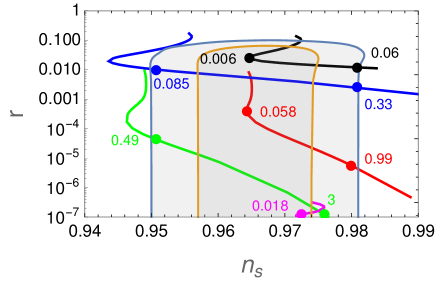
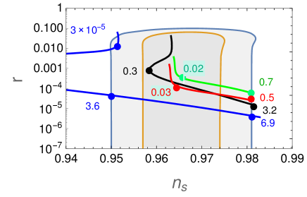
Figure 1: The spectral index $n_{s}$ and the tensor-to-scalar ratio $r$ in the plane $(n_{s},r)$ for different values of the dissipation ratio $Q_{*}$ (indicated by the numbers next to the curves), for the chaotic quartic potential (black line), hilltop (red line), Higgs potential (green line), chaotic sextic potential (blue line) and for the plateau sextic potential (magenta line). The contours are for the $68\%$ and $95\%$ C.L. results from Planck 2015. Panel (a) are the results for the cubic dissipation coefficient, while panel (b) gives the results when the dissipation coefficient is linear.

where $\lambda$ and $\gamma$ are free dimensionless constant parameters ($\lambda$ can be fixed by the normalization condition on the amplitude of the scalar power spectrum) and $v$ is the vacuum expectation value (VEV) with dimension of energy.

Both the chaotic potentials (quartic and sextic) are representative examples of large field models, and the quartic potential is a typical prototype potential used in many renormalizable scalar field theories. While in the CI picture these are examples of potentials unfavorable by the Planck data Planck2015 , they can be rehabilitated in the context of WI Bartrum:2013fia ; Bastero-Gil:2016qru ; Ramos:2013nsa . Instead, potentials like the hilltop, the Higgs and the plateau ones are typical examples of small field models of inflation and are found to be in agreement with the Planck data in both cold and warm inflation pictures Bartrum:2013oka .

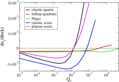
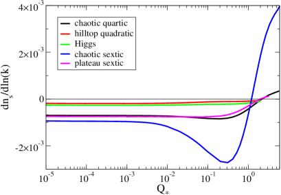
Figure 2: The running spectral index, $n_{s}^{\prime}$, as a function of the dissipation ratio $Q_{*}$. Panel (a) are the results for the cubic dissipation coefficient, while panel (b) gives the results when the dissipation coefficient is linear.

In order to produce $n_{s}$ predictions compatible with the latest CMB data for a wider range of $Q_{*}$ variation, we choose different setting values for the arbitrary parameters $\gamma$ and $v$. Thus, the vacuum expectation value $v$ for the plateau sextic potential Eq. (30) is set to $v=M_{P}$, while in the Higgs potential Eq. (29) we have assumed $v=13.2\,M_{P}$. In particular, the latter choice is a limiting value below which $n_{s}$ is at the border of the values constrained from Planck in CI model, i.e., $n_{s}<0.95$ for $v<13.2\,M_{P}$. We follow the same idea to choose the $\gamma$ value of the hilltop potential, depending on the type of dissipation coefficient. We assume $\gamma=0.0147$ for the cubic and $\gamma=0.025$ for the linear form of dissipation, respectively.

The plane $(n_{s},r)$ for each considered potentials and for the two different forms of the dissipation coefficient are shown in Fig. 1 for different values of $Q_{*}$. In the panel (a) we can see the prediction when a cubic dissipation coefficient is considered, while in the panel (b) we have the results for the linear dissipation form. The results for the plateau sextic potential does not appear in the

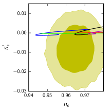
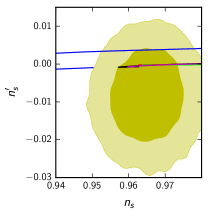
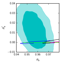
Figure 3: Marginalized joint $68\%$ and $95\%$ C.L. for the $\Lambda$CDM$+n_{s}^{\prime}$ model (yellow contours) and the $\Lambda$CDM$+n_{s}^{\prime}+n_{s}^{\prime\prime}$ model (cyan contours) from Planck TT+lowP data. The CL are compared with the WI theoretical predictions of the cubic dissipation regime (left column) and linear dissipation regime (right column). The color schemes for the curves refer to each of the inflaton potentials considered and are the same as the ones used in Fig. 2.

panel (b) since it produces values of $r$ well below the scale shown in the figure, with $r\lesssim 10^{-8}$. The smallest initial value considered for the dissipation ratio $Q_{*}$ is always $10^{-5}$ and its value increases up to the values shown at the most right side of the plots. We can see that all the curves show a decrease in $r$ when $Q_{*}$ increases. This is easily explained recalling the Eq. (22) and that, while the gravitational tensor modes remain unchanged, the scalar power spectrum is enhanced by the factor ${\cal F}(k/k_{*})$, Eq. (21). This is why, for example, the simple chaotic quartic or sextic potentials, which are discarded in the CI picture for their large tensor-to-scalar prediction, can be again in accordance with the observational data in the WI case. We also note that the results obtained for the linear dissipation coefficient allow a larger range for $Q_{*}$ in both the chaotic potentials, while for the hilltop and Higgs potentials we have an opposite behavior.

In Fig. 2 we show the running of the spectral index, $n_{s}^{\prime}$, as a function of the dissipation ratio $Q_{*}$ considering the cubic dissipation coefficient, panel (a), and for the linear dissipation coefficient, panel (b). We can see that the running value is always small and within the Planck ranges for any value of $Q_{*}$ and for each of the models we have considered. Noteworthy, $n_{s}^{\prime}$ remains negative for

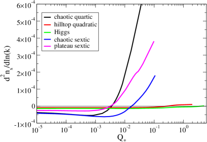
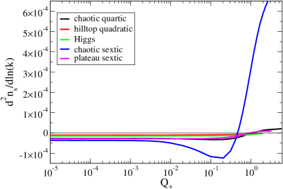
Figure 4: The running of the running, $n_{s}^{\prime\prime}$, as a function of the dissipation ratio $Q_{*}$. Panel (a) are the results for the cubic dissipation coefficient, while panel (b) gives the results when the dissipation coefficient is linear.

smaller values of the dissipation ratio and become positive for $Q_{*}\gtrsim 0.01$ when we assume a cubic dissipation regime, or $Q_{*}\gtrsim 1$ for the linear dissipation case. Also for the Higgs potential the $n_{s}^{\prime}$ turns positive for values of $Q_{*}$ that lie beyond the contours of the $(n_{s},r)$ plane of Fig. 1, which are out of our interest. The behaviors shown in Fig. 2 are very remarkable since the current Planck data constrain a tiny negative value for the running at $68\%$ CL when the extension with $n_{s}^{\prime}$ to the minimal model is considered, while prefer a tiny positive value when also $n_{s}^{\prime\prime}$ is assumed. In the CI model only negative values for the running are predicted, on the contrary in WI we are observing more possibilities.

In Fig. 3, the left panels always show the predictions for the cubic dissipation regime, while in the right panels are the results for the linear dissipation case. In panels (a) and (b) we plot the WI theoretical predictions compared with the two-dimensional confidence region of the ($n_{s}^{\prime}$, $n_{s}$) plan for the $\Lambda$CDM$+n_{s}^{\prime}$ model (yellow contours). The remaining (c)-(d) panels show the predictions for the $\Lambda$CDM$+n_{s}^{\prime}+n_{s}^{\prime\prime}$ model (cyan contours) from Planck TT+lowP data. We note that the running $n_{s}^{\prime}$ WI predictions are

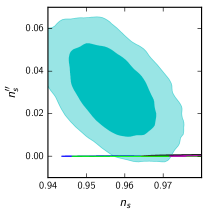
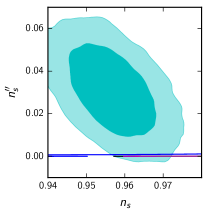
Figure 5: Marginalized joint $68\%$ and $95\%$ C.L. for the $\Lambda$CDM$+n_{s}^{\prime}+n_{s}^{\prime\prime}$ model from Planck TT+lowP data. The CL are compared with the WI theoretical predictions of the cubic dissipation regime (left column) and linear dissipation regime (right column). The color schemes for the curves (not easily distinguishable in the scale of the plots) refer to each of the inflaton potentials considered and are the same as the ones used in Fig. 2.

inside the $68\%$ CL, depending from the $Q_{*}$ value, for both the analysis.

We also show the running of the running $n_{s}^{\prime\prime}$ as a function of $Q_{*}$ in Fig. 4, when are considered the cubic and linear dissipation coefficients, respectively panels (a) and (b). Similarly to what happened for the running, also for the running of the running all the models starts with a small negative value, which then for some larger value of $Q_{*}$ become positive. Also in this case the Higgs potential becomes positive for much larger values of $Q_{*}$, not shown in the plots. The behaviours seen for $n_{s}^{\prime\prime}$ are very peculiar, since the results given by the CI single field models, as well as non-interacting multifield inflaton models, are naturally not capable of explaining a positive running of the running. In particular, all the models considered here predict in a CI context a negative $n_{s}^{\prime\prime}$ (see, e.g., Ref. Escudero:2015wba ). In the WI picture, however, our results show that we can achieve a positive $n_{s}^{\prime\prime}$, in accordance to what is indicated by the more recent CMB analysis Planck2015 ; Cabass:2016ldu (see also Ref. vandeBruck:2016rfv for a discussion of an alternative way of producing a positive $n_{s}^{\prime\prime}$ in a somewhat intricate two-field CI model). Noteworthy, the predicted value of $n_{s}^{\prime\prime}$ of Fig. 4 are very tiny, almost close to zero. In Fig. 5 we show the marginalized CL for the $\Lambda$CDM$+n_{s}^{\prime}+n_{s}^{\prime\prime}$ model compared with the WI theoretical predictions of the cubic dissipation regime, panel (a) and linear dissipation regime, panel (b). We can see that several analyzed values of $Q_{*}$ lie inside the $95\%$ CL.

For completeness, in Fig. 6 we show the running $n_{t}$ of the tensor spectrum, $\Delta_{T}(k)\propto k^{n_{t}}$, as a function of the tensor-to-scalar ratio $r$. The dissipation ratio $Q_{*}$ increases from $10^{-5}$ up the values shown in Fig. 1 and, consequently, the values of $r$ decrease for each potential treated. We already noticed that, in the WI context, the dissipation affects strongly the scalar curvature power

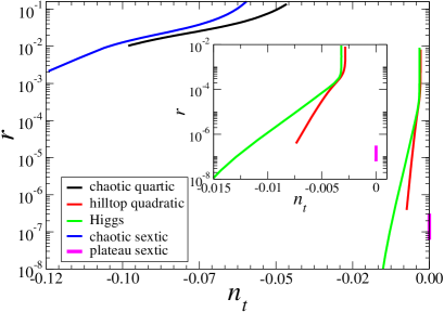
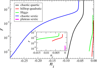
Figure 6: The tensor tilt $n_{t}$ and the tensor-to-scalar ratio $r$ in the plane $(n_{t},r)$ for different values of the dissipation ratio $Q_{*}$. Panel (a) are the results for the cubic dissipation coefficient, while panel (b) gives the results when the dissipation coefficient is linear. For both cases of dissipation, the plateau sextic potential (magenta line) have a too small $r\lesssim 10^{-8}$ and very small $n_{t}$ and whose results are barely seen in the scale of the figures.

spectrum while the tensors remain unaffected. Indeed, the WI only indirectly affects the tensors through the change of dynamics for the Hubble parameter, due to the presence of the radiation bath. Note that the consistency relation observed in CI, $r=-8n_{t}$, is modified in the WI picture. It become $r<8|n_{t}|$, again as a consequence of the enhancement factor Eq. (21) that affects WI but not CI.

The value of $r$ decreases for both the regimes with respect to the cold inflation, and this allows to a larger range of parameter values (temperature and dissipation) to enter in accordance with the Planck data. In this sense, the WI induces an increased degeneracy in the results for $r$ and $n_{s}$ for different types of inflaton potentials. The degeneracy can in principle be broken when we combine these results with those obtained for the other observables like the running and the running of the running of the spectral index, but these constraints are still

Table 1: The values of dissipation ratio $Q_{*}$ and $T_{*}/H_{*}$, along also the values of $r$, $n_{s}^{\prime}$ and $n_{s}^{\prime\prime}$, and the $\Delta\chi^{2}$ with respect to the minimal $\Lambda$CDM model when $n_{s}$ is fixed at the value $n_{s}\simeq 0.9655$, for each model considered in this work.

$V(\phi)$	$\Upsilon$	$Q_{*}$	$T_{*}/H_{*}$	$r$	$n_{s}^{\prime}$	$n_{s}^{\prime\prime}$	$\Delta\chi^{2}_{\rm min}$
quartic		$1.697\times 10^{-3}$	$7.246$	$0.036$	$-9.840\times 10^{-4}$	$-2.557\times 10^{-5}$	-0.2
sextic		$0.187$	$41.945$	$5.225\times 10^{-3}$	$1.540\times 10^{-3}$	$1.972\times 10^{-4}$	+0.3
hilltop	$\propto\frac{T^{3}}{\phi^{2}}$	$0.186$	$41.656$	$1.741\times 10^{-4}$	$-9.997\times 10^{-5}$	$-3.101\times 10^{-6}$	+0.1
Higgs		$1.417$	$214.829$	$2.317\times 10^{-6}$	$-1.857\times 10^{-4}$	$-4.333\times 10^{-6}$	-0.1
plateau sextic		$5.645\times 10^{-3}$	$10.766$	$1.085\times 10^{-7}$	$-4.692\times 10^{-4}$	$3.369\times 10^{-5}$	0
quartic		$1.256$	$273.472$	0 $1.27639\times 10^{-4}$	$-3.019\times 10^{-4}$	$4.156\times 10^{-6}$	0
sextic		$4.966$	$769.074$	$1.064\times 10^{-5}$	$3.731\times 10^{-3}$	$8.381\times 10^{-4}$	+0.7
hilltop	$\propto T$	$0.028$	$50.303$	$1.092\times 10^{-4}$	$-1.58837\times 10^{-4}$	$-1.028\times 10^{-5}$	0
Higgs		$0.020$	$44.492$	$2.947\times 10^{-4}$	$-2.50462\times 10^{-4}$	$-1.424\times 10^{-5}$	-0.1
plateau sextic		$0.810$	$210.187$	$4.448\times 10^{-9}$	$-3.862\times 10^{-4}$	$-2.708\times 10^{-6}$	0

too small and can remain within the Planck allowed ranges.

IV Analysis and Results

Let us now study the statistical viability of the WI cases of inflaton models considered in the previous section, for both the dissipation regimes defined by Eqs. (9) and (13), using the most up-to-date CMB data. To perform our analysis, we consider a minimal $\Lambda$CDM model and modify the standard primordial power-law spectrum following the equations for the WI picture. Therefore, we vary the usual cosmological parameters, namely, the physical baryon density, $\Omega_{b}h^{2}$, the physical cold dark matter density, $\Omega_{c}h^{2}$, the ratio between the sound horizon and the angular diameter distance at decoupling, $\theta$, and the optical depth, $\tau$. We do not use the primordial parameters $\mathcal{A}_{s}$ and $n_{s}$, respectively the scalar amplitude and the spectral index, since we parameterise the primordial spectrum as in Eq. (19). Both $P_{0}(k/k_{*})$ and ${\cal F}(k/k_{*})$ are obtained numerically for the studied potentials by solving the background equations in WI for different values of the the dissipation ratio $Q_{*}$. These values are calculated for the scales leaving the Hubble radius in an interval $\Delta N=5$ around the value $N_{*}$, where the pivot scale crosses the horizon. This corresponds to an analysis of $10$ e-folds of inflation, which is roughly the range of values of primordial expansion probed by the current CMB data. We note that the dissipation ratio $Q_{*}$, the temperature ratio $T_{*}/H_{*}$ and the amplitude $P_{0}(k/k_{*})$ of Eq. (19) are found to be linear with the scale for the considered potentials and for both the dissipation regimes. Hence, we can approximate them in our analysis with a power-law fitting without loss of information. Our parameterization is proved to be very accurate, taking into account higher order effects such as the running and the running of the running informations. In our analysis we also vary the nuisance foreground parameters Aghanim:2015xee and consider purely adiabatic initial conditions. The sum of neutrino masses is fixed to $0.06$ eV, and we limit the analysis to scalar perturbations with $k_{*}=0.05$ $\rm{Mpc}^{-1}$.

To obtain our results, we use a modified version of the CAMB camb to compute the theoretical CMB anisotropies spectrum in a WI context for different values of the dissipation ratio $Q_{*}$. In order to compare these theoretical predictions with observational data, we employ a Monte Carlo Markov Chain analysis via the publicly available package CosmoMC Lewis:2002ah . Finally, to maximize the likelihood and write our results, we use the Bound Optimization BY Quadratic Approximation (BOBYQA) algorithm Powell , which is an optimized method implemented in the CosmoMC code in order to minimize the $\chi^{2}$ value of the models.

We choose to use the second release of Planck data “TT+lowP”, namely the high multipole Planck temperature data (TT) from the 100-,143-, and 217-GHz half-mission TT cross-spectra and the low-$\ell$ data by the joint TT, EE, BB and TE likelihood (lowP) Aghanim:2015xee . We choose to not include high-$\ell$ polarization data since they have not a significant impact on the constraint of the $n_{s}^{\prime}$ and $n_{s}^{\prime\prime}$ parameters, as already found by the Planck Collaboration Planck2015 . Indeed, both these parameters affect more the low multipoles than the other scales. We also decide to not include tensor data in our analysis. Since the $r$ values of all the models we are going to analyze are inside the current $68\%$ C.L. of the TT+lowP data, it is reasonable to expect that tensor data do not add significant information.

As we saw in Fig. 1, the dissipative ratio $Q_{*}$ variation produces a significant change in the value of $n_{s}$ for each potential considered. Since the data show very accurate constraint on the $n_{s}$ parameter, we expect fine constraints also on $Q_{*}$. At the same time, the Planck data prefers $\simeq 0.9655$ as central value for $n_{s}$, so it is easy to suppose that the most preferred dissipative ratio is the one that guarantees that value. In our analysis we explore the wide range of $Q_{*}$ shown in Fig. 1, but for

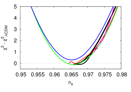
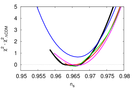
Figure 7: The behavior of the $\chi^{2}$ value as a function of the spectral index $n_{s}$ for the chaotic quartic potential (black line), hilltop (red line), Higgs potential (green line), chaotic sextic potential (blue line) and for the plateau sextic potential (magenta line). Panel (a): Results for the cubic dissipation coefficient. Panel (b): Results for the linear dissipation coefficient.

illustration we show in Tab. 1 the observational predictions when $n_{s}$ is fixed at the expected central value $n_{s}\simeq 0.9655$. The value of the $\Delta\chi^{2}$, with respect to the minimal $\Lambda$CDM data, is also quoted for illustration. We stress that this value cannot correspond to the best-fit value of the model, though it is still met for very close value. We note that the chaotic sextic model is the only one that produces, for the favorite $n_{s}$ value, a positive $n_{s}^{\prime}$ and $n_{s}^{\prime\prime}$. At the same time, it shows the worst $\Delta\chi^{2}$. This is due to the very small contribution of the running of the running, lesser than $10^{-4}$ for all the WI models. Indeed, as we just saw in the previous section for the $\Lambda$CDM+$n_{s}^{\prime}$ analysis, the data show a preference for negative value of the running when $n_{s}^{\prime\prime}$ is zero (or close to zero).

The results of our analysis are presented in Figs. 7 and  8, where we show the $\Delta\chi^{2}$ values of each considered

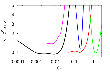
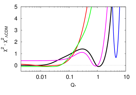
Figure 8: The behavior of the $\chi^{2}$ value as a function of the dissipation ratio $Q_{*}$ for the chaotic quartic potential (black line), hilltop (red line), Higgs potential (green line), chaotic sextic potential (blue line) and for the plateau sextic potential (magenta line). Panel (a): Results for the cubic dissipation coefficient. Panel (b): Results for the linear dissipation coefficient.

model, always with respect to the minimal $\Lambda$CDM model, as a function of the spectral index $n_{s}$ and in terms of the dissipative ratio $Q_{*}$, respectively. As before, in the panels (a) we show the results assuming the cubic dissipation, while in the panels (b) are the results for the linear dissipation case. In the Fig. 7 the variation of $\chi^{2}$ is of order of unity when the $n_{s}$ parameter value varies within its $1\sigma$ error, while rapidly increases until $\Delta\chi^{2}\sim 5$, for $n_{s}$ varying within $95\%$ CL. We also note that the minimum best fit of these WI models is compatible with the $\Lambda$CDM one. Noteworthy, the chaotic sextic model shows the worst $\Delta\chi^{2}$, which is seen more pronounced in the linear dissipation regime. The reason becomes clear looking the curves of this model in the panel (b) of Figs. 1 and 2, where we can note that only values of $3<Q*<6.5$ reconcile the $n_{s}$ into the $95\%$ C.L. of the Planck data,

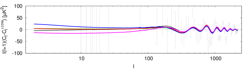
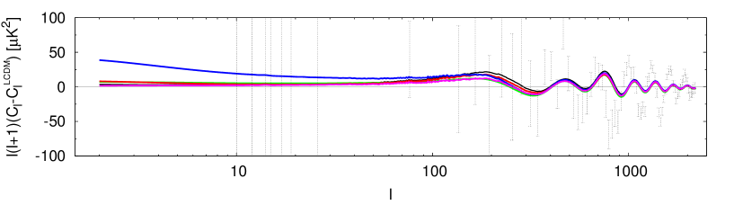
Figure 9: Temperature power spectrum residual plots for the best fit of the chaotic quartic potential (black line), hilltop (red line), Higgs potential (green line), chaotic sextic potential (blue line) and for the plateau sextic potential (magenta line) with respect to the $\Lambda$CDM model (grey line). Data shown are the TT+lowP (Planck 2015). Panel (a): Results for the cubic dissipation coefficient. Panel (b): Results for the linear dissipation coefficient.

but for values of $Q*>1$ it shows positive running, which is ruled out by the same data for the $\Lambda$CDM+$n_{s}^{\prime}$ analysis. The latter is assumed as reference since, as we have already mentioned above, for these WI models the running of the running $n_{s}^{\prime\prime}$ is too small and the data accuracy is not enough to detect the tiny signal. The incompatibility to satisfy both the observables causes the worse $\Delta\chi^{2}$. At the same time we note that there are values of $Q_{*}$, for all the other potentials, that allow combinations of the $n_{s}$ and its higher order parameters such that all the current observations are fulfilled. Finally, in Fig. 8 we can see that the significantly different behavior between the cubic and linear dissipation cases is reflected in a further preference for higher values of $Q_{*}$ in the latter for all the models, except for the hilltop and Higgs models.

The differences between the best fit temperature power spectrum of our analysis and the minimal $\Lambda$CDM model is shown in Fig. 9. Here, the best fit WI models are very close to the minimal $\Lambda$CDM predictions, with slightly different amplitude with respect to the simplest power-law potential. Our work shows that these slight variations are too small to be appreciated by the current observations with a $\chi^{2}$ statistical analysis. At the same time, the data well constrain the observables determined by the dissipation ratio value and we obtained the first estimate of how $Q_{*}$ affects the anisotropy temperature spectra. Also, we can comment that the two dissipation coefficient forms considered do not produce specific features in the spectrum. As already mentioned, we want to stress that as our WI parameterization takes into account one degree of freedom less than the $\Lambda$CDM model and ensures a best fit $\Delta\chi^{2}\sim 0$.

Finally, it is interesting to quote the current best fit value, in the CI context, of several inflaton potentials we have analyzed  Planck2015 . For instance, for the chaotic quartic potential model it was estimated $\Delta\chi^{2}=+43.3$ with respect to the $\Lambda$CDM model; for the hilltop potential $\Delta\chi^{2}=+4.4$ and for the Higgs potential $\Delta\chi^{2}=+5.5$. These values can be compared with the $\Delta\chi^{2}$ values shown in the Tab. 1, or in Figs 7 and 8. Then, our analysis gives a good indication of how the WI picture reconciles the different inflaton potentials considered, producing observables in agreement with the data.

V Conclusions

In this work we performed extended analysis of several representative inflaton potentials in a warm inflation scenario, covering both large and small field models. We obtain our results studying two different dissipation regimes, namely with the dissipation coefficient showing a cubic and linear dependence with the temperature of the thermal bath.

The dynamics leading to the dissipation coefficient with a cubic form emerges in what is usually referred as the low temperature regime of WI, where the inflaton is coupled to heavy intermediate fields that are in turn coupled to light radiation fields. The decay of the heavy intermediate fields into the light radiation fields produces the cubic dependence of the dissipation coefficient.  Berera:2008ar ; Bastero-Gil2011 ; BasteroGil:2012cm . The second dissipation regime we have considered is known in the literature as the high temperature regime of WI. Here the inflaton field directly couples to the radiation fields, yet preventing large thermal and radiative corrections to the inflaton potential, as a consequence of a collective symmetry breaking in the model construction. This leads to a dissipation coefficient that is linear in the temperature  Bastero-Gil:2016qru .

We achieve a parameterization of the primordial power spectrum able to take into account higher order effects as the running and the running of the running, and we analyze the observational predictions of the considered models in the two dissipation regimes described above. We show that the tensor modes are not affected by the dissipative dynamics, while the scalar spectra is modified by an additional enhancement term. Hence, the dissipation ratio $Q_{*}$ shows a significant impact on the spectral index $n_{s}$ and the tensor-to-scalar ratio $r$. It can reconcile the parameters value with the observation, i.e., a non detection of primordial gravity waves might be a hint of WI in the high dissipative regime ($Q_{*}\gtrsim 1$). In other words, a change of $Q_{*}$ allows a larger range of cosmological parameter values to enter in accordance with the Planck results. This degeneracy can in principle be broken combining these results with the constraints on the other observables. Other way is to study the non-Gaussianities, since in WI these have distinct features when compared with the CI picture Bastero-Gil:2014raa . We can also distinguish the regimes of weak dissipation $Q_{*}\ll 1$, with those of strong dissipation $Q_{*}\gtrsim 1$ through different shapes, unique to WI (for details, see, e.g., Ref. Bastero-Gil:2014raa ).

Intriguing, our studies show that both the running $n_{s}^{\prime}$ and the running of the running $n_{s}^{\prime\prime}$ assume negative or positive values depending on $Q_{*}$. These behaviors are in contrast with the CI results, where only negative values for $n_{s}^{\prime}$ and $n_{s}^{\prime\prime}$ are predicted. The WI picture is demonstrating a better versatility, where the parameter $Q_{*}$ (or, equivalently, the temperature of the thermal bath present during the WI dynamics) is the key parameter, and can achieve values able to better explain the current data.

We compared the predictions with the most up-to-date CMB data and we performed a statistical analysis to constrain the dissipative effects. The data well constrain the observables determined by the dissipation ratio value, and we get the first estimate of how $Q_{*}$ affects the anisotropy temperature power spectrum. Our results show the agreement between the WI picture with the Planck release, rehabilitating several forms of primordial potentials ruled out by the data in the CI context. At the same time, our analysis show that the chaotic sextic model is unable to describe the current data, since there is not a value of $Q_{*}$ that is able to satisfy simultaneously the values required for the spectral index and its running. Despite the values for $n_{s}^{\prime\prime}$ obtained for all the models are still to small to be of relevance, we note that its magnitude tends to increase with the gain in dissipation value. It is a feature that can eventually be explored in future model building in WI. At the same time, the current constraints on the higher order parameters are still too wide, improvements in the data are need to update our results.

- (1) N. Aghanim et al. [Planck Collaboration], Planck 2015 results. XI. CMB power spectra, likelihoods, and robustness of parameters, Astron. Astrophys. 594, A11 (2016).
- (2) P. A. R. Ade et al. [Planck Collaboration], Planck 2015 results. XX. Constraints on inflation, Astron. Astrophys. 594, A20 (2016).
- (3) P. A. R. Ade et al. [Planck Collaboration], Planck 2015 results. XVII. Constraints on primordial non-Gaussianity, Astron. Astrophys. 594, A17 (2016).
- (4) A. H. Guth, The Inflationary Universe: A Possible Solution to the Horizon and Flatness Problems, Phys. Rev. D 23, 347 (1981).
- (5) K. Sato, Cosmological Baryon Number Domain Structure and the First Order Phase Transition of a Vacuum, Phys. Lett. B 99, 66 (1981).
- (6) A. Albrecht and P. J. Steinhardt, Cosmology for Grand Unified Theories with Radiatively Induced Symmetry Breaking, Phys. Rev. Lett. 48, 1220 (1982).
- (7) A. D. Linde, A New Inflationary Universe Scenario: A Possible Solution of the Horizon, Flatness, Homogeneity, Isotropy and Primordial Monopole Problems, Phys. Lett. B 108, 389 (1982).
- (8) A. D. Linde, Chaotic Inflation, Phys. Lett. B 129, 177 (1983).
- (9) A. Berera, Warm inflation, Phys. Rev. Lett. 75, 3218 (1995).
- (10) S. Bartrum, M. Bastero-Gil, A. Berera, R. Cerezo, R. O. Ramos and J. G. Rosa, The importance of being warm (during inflation), Phys. Lett. B 732, 116 (2014). [arXiv:1307.5868 [hep-ph]].
- (11) S. Bartrum, A. Berera and J. G. Rosa, Warming up for Planck, JCAP 06 (2013) 025.
- (12) M. Bastero-Gil, A. Berera, I. G. Moss and R. O. Ramos, Theory of non-Gaussianity in warm inflation, JCAP 12 (2014) 008.
- (13) R. O. Ramos and L. A. da Silva, Power spectrum for inflation models with quantum and thermal noises, JCAP 03 (2013) 032.
- (14) M. Bastero-Gil, A. Berera, R. O. Ramos and J. G. Rosa, Observational implications of mattergenesis during inflation, JCAP 10 (2014) 053.
- (15) R. Herrera, M. Olivares and N. Videla, General dissipative coefficient in warm intermediate inflation in loop quantum cosmology in light of Planck and BICEP2, Int. J. Mod. Phys. D 23 (2014) no.10, 1450080.
- (16) G. Panotopoulos and N. Videla, Warm inflationary universe model in light of Planck 2015 results, Eur. Phys. J. C 75 (2015) no.11, 525.
- (17) M. Bastero-Gil, A. Berera and N. Kronberg, Exploring the Parameter Space of Warm-Inflation Models, JCAP 12 (2015) 046.
- (18) R. Herrera, N. Videla and M. Olivares, Warm intermediate inflation in the Randall–Sundrum II model in the light of Planck 2015 and BICEP2 results: a general dissipative coefficient, Eur. Phys. J. C 75 (2015) no.5, 205.
- (19) L. Visinelli, Observational Constraints on Monomial Warm Inflation, JCAP 07 (2016) 054.
- (20) X. M. Zhang, H. Y. Ma, P. C. Chu, J. T. Liu and J. Y. Zhu, Primordial non-Gaussianity in warm inflation using formalism, JCAP 03 (2016) 059.
- (21) A. Berera, I. G. Moss and R. O. Ramos, Warm Inflation and its Microphysical Basis, Rept. Prog. Phys. 72, 026901 (2009).
- (22) M. Bastero-Gil and A. Berera, Warm inflation model building, Int. J. Mod. Phys. A 24, 2207 (2009).
- (23) C. -H. Wu, K. -W. Ng, W. Lee, D. -S. Lee and Y. -Y. Charng, Quantum noise and a low cosmic microwave background quadrupole, J. Cosmol. Astropart. Phys. 02, 006 (2007).
- (24) W. Lee, K. -W. Ng, I-C. Wang and C. -H. Wu, Trapping effects on inflation, Phys. Rev. D 84, 063527 (2011).
- (25) G. C. Liu, K. W. Ng and I. C. Wang, Naturally large tensor-to-scalar ratio in inflation, Phys. Rev. D 90, 103531 (2014).
- (26) M. Bastero-Gil, A. Berera, I. G. Moss and R. O. Ramos, Cosmological fluctuations of a random field and radiation fluid, JCAP 05 (2014) 004.
- (27) G. S. Vicente, L. A. da Silva and R. O. Ramos, Eternal inflation in a dissipative and radiation environment: Heated demise of eternity, Phys. Rev. D 93, no. 6, 063509 (2016).
- (28) A. N. Taylor and A. Berera, Perturbation spectra in the warm inflationary scenario, Phys. Rev. D 62, 083517 (2000).
- (29) L. M. H. Hall, I. G. Moss and A. Berera, Scalar perturbation spectra from warm inflation, Phys. Rev. D 69, 083525 (2004).
- (30) D. Lyth and A. Liddle, The Primordial Density Perturbation: Cosmology, Inflation and the Origin of Structure (Cambridge University Press, Cambridge, 2009).
- (31) M. Bastero-Gil, A. Berera and R. O. Ramos, Dissipation coefficients from scalar and fermion quantum field interactions, JCAP 09 (2011) 033.
- (32) M. Bastero-Gil, A. Berera, R. O. Ramos and J. G. Rosa, General dissipation coefficient in low-temperature warm inflation, JCAP 01 (2013) 016.
- (33) A. Berera, M. Gleiser and R. O. Ramos, Strong dissipative behavior in quantum field theory, Phys. Rev. D 58, 123508 (1998).
- (34) J. Yokoyama and A. D. Linde, Is warm inflation possible?, Phys. Rev. D 60, 083509 (1999).
- (35) A. Berera, M. Gleiser and R. O. Ramos, A First principles warm inflation model that solves the cosmological horizon / flatness problems, Phys. Rev. Lett. 83, 264 (1999).
- (36) M. Bastero-Gil, A. Berera, R. O. Ramos and J. G. Rosa, Warm Little Inflaton, Phys. Rev. Lett. 117, no. 15, 151301 (2016).
- (37) M. Schmaltz and D. Tucker-Smith, Little Higgs review, Ann. Rev. Nucl. Part. Sci. 55, 229 (2005).
- (38) M. Escudero, H. Ramírez, L. Boubekeur, E. Giusarma and O. Mena, The present and future of the most favoured inflationary models after 2015, JCAP 02 (2016) 020.
- (39) G. Cabass, E. Di Valentino, A. Melchiorri, E. Pajer and J. Silk, Running the running, Phys. Rev. D 94, no. 2, 023523 (2016).
- (40) C. van de Bruck and C. Longden, Running of the Running and Entropy Perturbations During Inflation, Phys. Rev. D 94, no. 2, 021301 (2016).
- (41) A. Berera and R. O. Ramos, Construction of a robust warm inflation mechanism, Phys. Lett. B 567 (2003) 294.
- (42) C. Graham and I. G. Moss, Density fluctuations from warm inflation, JCAP 07 (2009) 013.
- (43) M. Bastero-Gil, A. Berera and R. O. Ramos, Shear viscous effects on the primordial power spectrum from warm inflation, JCAP 07 (2011) 030.
- (44) R. O. Ramos and S. Andrade, Final stages of warm inflation and the connection with the radiation domination regime, work in progress.
- (45) P. A. R. Ade et al. [BICEP2 and Planck Collaborations], Joint Analysis of BICEP2/ and Data, Phys. Rev. Lett. 114, 101301 (2015).
- (46) A. Lewis, A. Challinor, and A. Lasenby, Efficient Computation of CMB anisotropies in closed FRW models, Astrophys. J. 538, 473 (2000).
- (47) A. Lewis and S. Bridle, Cosmological parameters from CMB and other data: A Monte Carlo approach, Phys. Rev. D 66, 103511 (2002).
- (48) M. J. D. Powell, The BOBYQA algorithm for bound constrained optimization without derivatives , University of Cambridge Report No. DAMTP 2009/NA06.