Lorentz violation and deep inelastic scattering

Abstract

The effects of quark-sector Lorentz violation on deep inelastic electron-proton scattering are studied. We show that existing data can be used to establish first constraints on numerous coefficients for Lorentz violation in the quark sector at an estimated sensitivity of parts in a million.

1 Introduction

Deep inelastic scattering (DIS) provides key experimental evidence for the existence of quarks and the validity of quantum chromodynamics (QCD). In early experiments on electron-proton scattering, the DIS cross section was discovered to vary only weakly with momentum transfer [1], and the invariance of the DIS form factors under scaling [2] revealed that nucleons contain partons [3]. Subsequent DIS studies with electrons and neutrinos have confirmed this picture and verified predictions of QCD, and DIS continues to be an essential tool in searches for new physics [4].

One proposal for new physics is tiny observable violations of Lorentz invariance, which could emerge as a byproduct of the unification of gravity and quantum physics in a Planck-scale theory such as strings [5]. Many sensitive searches for Lorentz violations have been performed in recent years, spanning most sectors of the Standard Model (SM) as well as gravity [6]. However, direct information about the Lorentz properties of quarks is comparatively difficult to obtain. In the present work, we investigate the prospects of using DIS as a tool to search for Lorentz violation. We obtain dominant Lorentz-violating corrections to the DIS cross section for electron-proton scattering and use data from the Hadronen-Elektronen Ring Anlage (HERA) [7] to estimate attainable sensitivities in a dedicated analysis searching for Lorentz violation.

Our treatment is based on techniques from effective field theory, which is appropriate for investigating suppressed signals from an experimentally inaccessible energy scale [8]. The realistic effective field theory for general Lorentz violation is known as the Standard-Model Extension (SME) [9, 10]. Each Lorentz-violating term in the SME action is a coordinate-independent contraction of a coefficient for Lorentz violation with a Lorentz-violating operator, which can be specified in part by its mass dimension $d$. Adding all Lorentz-violating terms to the action for General Relativity coupled to the Standard Model produces the SME action. Restricting attention to terms with $d\leq 4$ in Minkowski spacetime yields an action that is power-counting renormalizable, called the minimal SME. In realistic effective field theory, violation of CPT symmetry implies Lorentz violation [9, 11], so the SME also characterizes general effects of CPT violation. For reviews of the SME see, for example, Refs. [6, 12]. Here, we focus attention on the quark sector of the minimal SME, seeking to identify its predictions for DIS.

One way to access quark-sector SME coefficients is to take advantage of the interferometric nature of neutral-meson propagation [13]. Studies of kaon oscillations provide sensitivity to certain SME coefficients for CPT violation involving the $d$ and $s$ quarks [14], while oscillations of $D$, $B_{d}$, and $B_{s}$ mesons have been used to constrain CPT violation involving also the $u$, $c$, and $b$ quarks [15]. The $t$ quark decays before hadronizing and so its Lorentz properties cannot be investigated via interferometric methods, but observations of the production and decay of $t$-$\overline{t}$ pairs have been used to constrain SME coefficients for CPT-even Lorentz violation in the $t$-quark sector [16], and coefficients for CPT-odd Lorentz violation are accessible to studies of single-$t$ production and decay [17]. A few ultrarelativistic constraints on quark-sector coefficients have also been obtained from high-energy cosmic rays [18].

The primary goal of the present work is to show explicitly that electron-proton DIS can access spin-independent and CPT-even Lorentz violation involving $u$ and $d$ quarks, about which direct information is lacking in the literature. Indirect clues can be gleaned from other experiments involving nuclei or hadrons [6], but extracting direct quark-sector bounds from these requires disentangling possible Lorentz-violating effects from quarks, gluons, and sea constituents. Theoretical techniques such as Lorentz-violating chiral perturbation theory, which to date have been used to interrelate various hadron SME coefficients [19], could in principle also shed light on this issue. In any event, electron-proton DIS is of particular interest in this context because it is well measured, can be calculated with sufficient accuracy, and is comparatively simple in that only one of the two colliding species involves quarks.

2 Setup

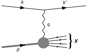
Figure 1: DIS of an electron (momentum $k^{\mu}$) off a proton (momentum $p^{\mu}$).

Since DIS is a high-energy process with momentum transfer greater than the proton mass, asymptotic freedom allows a perturbative treatment. At zeroth order in the strong coupling constant $g_{s}$, the interactions among quarks are neglected and the photon exchanged between the electron and the proton interacts with partons carrying a fraction of the proton total momentum. We focus on calculating the tree-level impact of Lorentz violation on this process, shown in Fig. 1.

For simplicity and definiteness, we limit attention to dominant effects in unpolarized electron-proton DIS and we neglect possible quark flavor-changing couplings. It is reasonable also to neglect electron- and photon-sector Lorentz violation, which are constrained well below levels attainable here [6]. The primary Lorentz-violating behavior can therefore be expected to arise from spin-independent CPT-even operators in the quark sector of the minimal SME. Including the two valence-quark flavors $f=u,d$ for the proton, the relevant part of the Lagrange density for Lorentz-violating QCD augmented by electromagnetic couplings [9] is then

$${\cal L}\supset\sum_{f=u,d}(\eta^{\mu\nu}+c^{\mu\nu}_{f})\overline{\psi}_{f}({\textstyle{1\over 2}}\gamma_{\mu}i\hskip-4.0pt\stackrel{{\scriptstyle\leftrightarrow}}{{\partial}}_{\nu}-q_{f}\gamma_{\mu}A_{\nu})\psi_{f}.$$ (1)

The dimensionless SME coefficients $c^{\mu\nu}_{f}$ control the magnitude of the Lorentz violation and can be taken as constant in an inertial frame in the vicinity of the Earth [9], which insures energy and momentum remain conserved. The coefficients modify the dispersion relation of the quarks, which propagate along pseudo-Finsler geodesics [20]. In the high-energy limit $Q^{2}=-q^{2}\gg M^{2}$, where $M$ is the mass of the proton, we can disregard the strong interactions and view the quarks as interacting only with the photon through their charges $q_{f}$. Nonetheless, the couplings in ${\cal L}$ reveal that the DIS cross section is affected by the quark-sector SME coefficients $c_{f}^{\mu\nu}$ in Lorentz-violating QCD.

The form of the Lagrange density ${\cal L}$ is simplified by the possibility of performing coordinate choices and field redefinitions that leave unaffected the observable physics [9, 10, 21]. For example, the contractions in the Maxwell term $-{\textstyle{1\over 4}}F_{\mu\nu}F^{\mu\nu}$ could in principle be performed with an effective metric involving the photon-sector coefficient $(k_{F})_{\alpha}{}^{\mu\alpha\nu}$ for Lorentz violation, but a suitable choice of coordinates can always absorb this into the coefficients $c_{f}^{\mu\nu}$ and the corresponding electron-sector coefficient $c_{e}^{\mu\nu}$. If desired, the general case can be recovered via the substitutions $c_{f}^{\mu\nu}\to c_{f}^{\mu\nu}+{\textstyle{1\over 2}}(k_{F})_{\alpha}{}^{\mu\alpha\nu}$ and $c_{e}^{\mu\nu}\to c_{e}^{\mu\nu}+{\textstyle{1\over 2}}(k_{F})_{\alpha}{}^{\mu\alpha\nu}$. In this context, disregarding Lorentz violation in the electron and photon sectors amounts to assuming that the combination $c_{e}^{\mu\nu}+{\textstyle{1\over 2}}(k_{F})_{\alpha}{}^{\mu\alpha\nu}$ is negligible based on existing precision tests of Lorentz invariance [6]. Field redefinitions also insure that spin-independent CPT-odd effects are unobservable at this level, and they imply that the coefficients $c_{f}^{\mu\nu}$ can be taken as symmetric without loss of generality. The trace $\eta_{\mu\nu}c_{f}^{\mu\nu}$ produces no Lorentz-violating effects and can be set to zero. The Lorentz-violating physics of interest here is therefore controlled by nine independent components of $c_{f}^{\mu\nu}$ for each quark flavor $f$.

To initiate the calculation, we first consider the DIS amplitude of Fig. 1 for a single quark of flavor $f$,

$$i{\cal M}=-4\pi i\alpha~{}\overline{u}(k^{\prime})\gamma^{\mu}u(k)~{}\frac{\eta_{\mu\nu}}{q^{2}}\int d^{4}x~{}e^{iq\cdot x}\langle X|J^{\nu}(x)|p\rangle,$$ (2)

where $\alpha$ is the fine structure constant, $J^{\mu}(x)=q_{f}\overline{\psi}_{f}(x)\Gamma_{f}^{\mu}\psi_{f}(x)$ is the quark electromagnetic current with $\Gamma_{f}^{\mu}=\gamma^{\mu}+c^{\nu\mu}_{f}\gamma_{\nu}$, and where $|p\rangle$ and $|X\rangle$ are interaction-picture kets for the proton and the final-state hadrons, respectively. Squaring this amplitude and summing over all possible final states $X$ gives

$$\hskip-20.0pt\sum_{X}\int d\Pi_{X}|{\cal M}|^{2} \hskip-5.0pt= \hskip-5.0pt\frac{16\pi\alpha^{2}}{q^{4}}\big{[}\overline{u}(k)\gamma^{\nu}u(k^{\prime})~{}\overline{u}(k^{\prime})\gamma^{\mu}u(k)\big{]}$$ (3)

$$\hskip-5.0pt\times\sum_{X}\int d\Pi_{X}\langle p|J_{\nu}(-q)|X\rangle\langle X|J_{\mu}(q)|p\rangle,$$

where $J^{\mu}(q)$ is the Fourier transform of the current. After averaging over the spins as required for an unpolarized cross section, the term in brackets involving the electron-photon interaction yields the electron tensor $L^{\mu\nu}=2(k^{\mu}k^{\prime\nu}+k^{\nu}k^{\prime\mu}-k\cdot k^{\prime}\eta^{\mu\nu})$. The part involving the sum over $X$ corresponds to the photon-proton interaction and depends on the quark-sector coefficients for Lorentz violation via the current $J^{\mu}(q)$. It is related to the proton tensor

$$W^{\mu\nu}=i\int d^{4}x~{}e^{iq\cdot x}\langle p|J^{\mu}(x)J^{\nu}(0)|p\rangle$$ (4)

via the optical theorem,

$$\sum_{X}\int d\Pi_{X}\langle p|J_{\nu}(-q)|X\rangle\langle X|J_{\mu}(q)|p\rangle=2~{}\hbox{Im}\,W_{\mu\nu},$$ (5)

as illustrated in Fig. 2. The proton tensor (4) contains the information about the photon-proton interaction and interactions among the proton constituents.

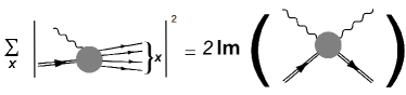
Figure 2: Optical theorem for the photon-proton interaction.

To obtain the unpolarized DIS differential cross section from the spin-averaged squared amplitude, we must divide by the flux factor $F$. Typically, care is required in defining $F$ in Lorentz-violating situations because it is frame dependent. To write $F$ in terms of the Mandelstam variable $s$ requires using the momentum-velocity relation, which is modified in the presence of Lorentz violation [22]. However, the flux factor here is associated with the initial electron and proton states, while the Lorentz violation concerns only the internal structure of the proton. The short-wavelength photon involved in DIS sees only the quark substructure, and so the flux factor can be taken to be $F=2s=2(k+p)^{2}$ as usual. In effect, since proton-sector Lorentz violation is well constrained [6], we can neglect it for present purposes.

The differential cross section depends on the phase-space variables for the scattered electron. The trajectory of the final electron lies along a cone of opening angle $\theta$ equal to the scattering angle. In the Lorentz-invariant case, the physics is independent of the azimuthal angle $\phi$ around this cone or, equivalently, of the orientation of the plane defined by the incoming and scattered electron. However, in the presence of Lorentz violation, the physics depends on the direction of travel of the scattered quark relative to $c_{f}^{\mu\nu}$, which via energy-momentum conservation is equivalent to dependence on $\phi$. The conventional two dimensionless variables used to characterize the phase space, Bjorken $x$ and $y$, must therefore be supplemented with a third variable corresponding to $\phi$. While this third variable might be defined in a frame-independent way using products of $c_{f}^{\mu\nu}$ with the 4-momenta, it is more transparent for present purposes to work directly in a specified frame. For definiteness, we adopt a detector frame having $z$ axis in the direction of the incoming electron, with the 4-momenta of the incoming electron, incoming proton, and outgoing electron given by $k^{\mu}=E(1,\hat{k})$, $p^{\mu}=E_{p}(1,-\hat{k})$, and $k^{\prime}=E^{\prime}(1,\hat{k}^{\prime})$, respectively, where $\hat{k}=(0,0,1)$, $\hat{k}^{\prime}=(\sin\theta\cos\phi,\sin\theta\sin\phi,\cos\theta)$. The standard $x$ and $y$ variables are

$$x \hskip-5.0pt= \hskip-5.0pt\frac{-q^{2}}{2p\cdot q}=\frac{E^{\prime 2}}{4EE_{p}}\frac{\sin^{2}\theta}{y(1-y)},$$

$$y \hskip-5.0pt= \hskip-5.0pt\frac{p\cdot q}{p\cdot k}=1-\frac{E^{\prime}}{2E}(1+\cos\theta),$$ (6)

and we choose $x$, $y$, and $\phi$ to parametrize the phase space for the differential cross section.

With the above considerations, the unpolarized differential cross section takes the form

$$\frac{d\sigma}{dxdyd\phi}=\frac{\alpha^{2}y}{2\pi q^{4}}L^{\mu\nu}~{}\hbox{Im}\,W_{\mu\nu}.$$ (7)

The spin average in $W^{\mu\nu}$ is understood. The form of $W^{\mu\nu}$ can be determined perturbatively, as the strong interaction is subdominant for $Q^{2}=-q^{2}\gg M^{2}$. One standard method is to write a general tensorial structure for the vectors $p$ and $q$, using the Ward identities to fix its form. In the presence of Lorentz violation, this approach is involved because the coefficients $c^{\mu\nu}_{f}$ can also appear. Instead, we proceed below using the optical theorem and the Cutkosky rules, and we confirm the results via an alternative approach based on the operator-product expansion (OPE) in Sec. 4.

3 Cross section

The parton model can be used to calculate the explicit form of the proton tensor $W^{\mu\nu}$. In this approach, the photon interacts only with a parton $f$ in the state $|\xi p\rangle$ carrying a fraction $\xi$ of the proton 4-momentum $p$,

$$W^{\mu\nu}\approx i\int d^{4}x~{}e^{iq\cdot x}\hskip-5.0pt\int^{1}_{0}d\xi\sum_{f}\frac{f_{f}(\xi)}{\xi}\langle\xi p|J^{\mu}(x)J^{\nu}(0)|\xi p\rangle.$$ (8)

Here, the parton distribution function (PDF) $f_{f}(\xi)$ is the probability of finding a parton $f$ carrying a momentum $\xi p$. Both quarks and antiquarks of species $f$ are included in the sum, and the notation suppresses the $Q^{2}$ dependence of the PDF for simplicity. The parton propagates according to the Lorentz-violating dispersion relation, and the integral over $\xi$ allows for all possible fractions of $p$. In this approach, we take the dominant effects from Lorentz violation as arising in the matrix element and neglect possible effects in the PDF. Studying these effects is an interesting open challenge, although they are unlikely to change the order of magnitudes of the sensitivities estimated below. Note that the results obtained in this section using the parton expression (8) are supported by the OPE evaluation of Eq. (4) presented in Sec. 4.

Inserting the explicit form of $J^{\mu}$, applying Wick’s theorem at zeroth order in $g_{s}$, converting to momentum space, and taking the average over spins yields

$$\hskip-20.0ptW^{\mu\nu} \hskip-5.0pt= \hskip-5.0pt-{\textstyle{1\over 2}}\int^{1}_{0}d\xi\sum_{f}q^{2}_{f}{{f_{f}(\xi)}\over{\xi}}{{{\rm tr}~{}[\xi\Gamma_{f}^{\alpha}p_{\alpha}\Gamma_{f}^{\mu}(\xi\Gamma_{f}^{\beta}p_{\beta}+\Gamma_{f}^{\beta}q_{\beta})\Gamma_{f}^{\nu}]}\over{(\xi\Gamma_{f}^{\beta}p_{\beta}+\Gamma_{f}^{\beta}q_{\beta})^{2}+i\epsilon}}$$ (9)

$$+(\mu\leftrightarrow\nu,q\leftrightarrow-q).$$

In calculating the trace, terms beyond first order in $c_{f}^{\mu\nu}$ can be neglected.

The propagator denominator can be written as

$$(\xi\Gamma_{f}^{\beta}p_{\beta}+\Gamma_{f}^{\beta}q_{\beta})^{2}+i\epsilon \hskip-5.0pt= \hskip-5.0pt(\xi p+q)^{2}+2c_{f}^{\xi p+q\ \xi p+q}+i\epsilon$$ (10)

$$\hskip-5.0pt\approx \hskip-5.0pt-Q^{2}+2\xi p\cdot q+2c_{f}^{qq}$$

$$+2\xi(c_{f}^{qp}+c_{f}^{pq})+2\xi^{2}c_{f}^{pp}+i\epsilon$$

$$\hskip-5.0pt= \hskip-5.0pt\widetilde{q}^{2}+2\xi\widetilde{p}\cdot\widetilde{q}+2\xi^{2}c_{f}^{pp}+i\epsilon,$$

where we introduced the notation $c_{f}^{\mu\alpha}p_{\alpha}\equiv c_{f}^{\mu p}$ and $\widetilde{p}^{\mu}\equiv p^{\mu}+c_{f}^{\mu p}$. We neglect terms proportional to the proton mass $M$ because $M^{2}\ll Q^{2}$ and $M^{2}\ll 2p\cdot q$ in the DIS limit. Note that the term $c_{f}^{pp}$ can be neglected only in the rest frame of the proton.

The sole contribution to the imaginary part of the proton tensor comes from the propagator term shown explicitly in Eq. (9),

$$\hskip-20.0pt\hbox{Im}\,\left(\frac{-1}{(\xi\Gamma_{f}^{\beta}p_{\beta}+\Gamma_{f}^{\beta}q_{\beta})^{2}+i\epsilon}\right) \hskip-5.0pt= \hskip-5.0pt\pi\delta(-\widetilde{Q}^{2}+2\xi\widetilde{p}\cdot\widetilde{q}+2\xi^{2}c_{f}^{pp})$$ (11)

$$\hskip-5.0pt=\delta_{f}\delta(\xi-x_{f}^{\prime}),$$

where only the relevant root for $\xi$ and terms linear in $c_{f}^{\mu\nu}$ are kept. Here,

$$\delta_{f}=\frac{\pi}{ys}\left(1-\frac{2}{ys}(c^{pq}_{f}+c^{qp}_{f}+2xc^{pp}_{f})\right),$$ (12)

and $x_{f}^{\prime}=x-x_{f}$ is the Bjorken $x$ shifted by a factor

$$x_{f}=\frac{2}{ys}(c_{f}^{qq}+xc_{f}^{pq}+xc_{f}^{qp}+x^{2}c_{f}^{pp}),$$ (13)

with $s\approx 2k\cdot p$. The corresponding delta function for the other propagator term has no zeros and so gives no contribution to the DIS cross section.

To obtain the DIS differential cross section, we first contract the imaginary part of the proton tensor with $L^{\mu\nu}$ and then evaluate the $\xi$ integral. This gives

$$\hskip-20.0pt\frac{d\sigma}{dxdyd\phi} \hskip-5.0pt= \hskip-5.0pt\frac{\alpha^{2}}{q^{4}}\sum_{f}F_{2f}\Bigg{[}\frac{ys^{2}}{\pi}(1+(1-y)^{2})\delta_{f}+\frac{y^{2}s}{x}x_{f}$$ (14)

$$-\frac{4M^{2}}{s}(c_{f}^{kk^{\prime}}+c_{f}^{k^{\prime}k})+4(c_{f}^{k^{\prime}p}+c_{f}^{pk^{\prime}})+\frac{4}{x}(1-y)c_{f}^{kk}$$

$$-4xyc_{f}^{pp}-\frac{4}{x}c_{f}^{k^{\prime}k^{\prime}}+4(1-y)(c_{f}^{kp}+c_{f}^{pk})\Bigg{]},$$

where

$$F_{2f}=q^{2}_{f}f_{f}(x^{\prime}_{f})x^{\prime}_{f}$$ (15)

represents the contribution from a parton $f$ to the proton form factor, incorporating Lorentz-violation effects.

For large momentum transfer $Q^{2}\mathrel{\hbox to0.0pt{\lower 4.0pt\hbox{\hskip 1.0pt$\sim$}\hss}\raise 1.0pt\hbox{$>$}}m^{2}_{Z}$, where $m_{Z}$ is the $Z^{0}$-boson mass, $Z^{0}$ exchange must be included in the DIS process of Fig. 1. The squared amplitude $|{\cal M}|^{2}$ in the expression (3) then takes the form $|{\cal M}|^{2}=|{\cal M}_{\gamma}|^{2}+{\cal M}^{*}_{\gamma}{\cal M}_{Z}+{\cal M}^{*}_{Z}{\cal M}_{\gamma}+|{\cal M}_{Z}|^{2}$, where the indices $\gamma$ and $Z^{0}$ denote photon and $Z^{0}$ exchanges, respectively. This yields three additional pieces for both the proton and the electron tensors. The propagator $1/q^{4}$ in the cross section (7) is replaced by $(q^{2}-m_{Z}^{2})/(q^{2}[(q^{2}-m_{Z}^{2})^{2}+\Gamma_{Z}^{2}m_{Z}^{2}])$ for the two interference terms, while the propagator becomes $1/[(q^{2}-m_{Z}^{2})^{2}+\Gamma_{Z}^{2}m_{Z}^{2}]$ for the $|{\cal M}_{Z}|^{2}$ term, where $\Gamma_{Z}$ is the $Z^{0}$ width. After some calculation, we find the full cross section takes the form

$$\hskip-20.0pt\frac{d\sigma}{dxdyd\phi} \hskip-5.0pt= \hskip-5.0pt-\frac{\alpha^{2}y}{\pi q^{4}}\sum_{f}\frac{q^{2}_{f}f_{f}(x^{\prime}_{f})}{x^{\prime}_{f}}\delta_{f}L^{\mu\nu}\omega^{f}_{\mu\nu}$$ (16)

$$\hskip-20.0pt-\frac{\alpha^{2}y(1-m_{Z}^{2}/q^{2})}{\pi[(q^{2}-m_{Z}^{2})^{2}+\Gamma_{Z}^{2}m_{Z}^{2}]}\sum_{f}\frac{q_{f}f_{f}(x^{\prime}_{f})T^{f}_{3}}{x^{\prime}_{f}}\delta_{f}$$

$$\times\left(v_{f}(\theta_{W})v_{e}(\theta_{W})L^{\mu\nu}\omega^{f}_{\mu\nu}-\frac{x^{\prime}_{f}sQ^{2}}{4s^{2}_{W}c^{2}_{W}}(y-2)\right)$$

$$\hskip-20.0pt-\frac{\alpha^{2}y}{16\pi[(q^{2}-m_{Z}^{2})^{2}+\Gamma_{Z}^{2}m_{Z}^{2}]}\sum_{f}\frac{f_{f}(x^{\prime}_{f})}{x^{\prime}_{f}}\delta_{f}$$

$$\times\Bigg{[}\left(v^{2}_{f}(\theta_{W})+\frac{1}{4s^{2}_{W}c^{2}_{W}}\right)\left(v^{2}_{e}(\theta_{W})+\frac{1}{4s^{2}_{W}c^{2}_{W}}\right)L^{\mu\nu}\omega^{f}_{\mu\nu}$$

$$\hskip 15.0pt+\frac{x^{\prime}_{f}sQ^{2}}{s^{2}_{W}c^{2}_{W}}v_{f}(\theta_{W})v_{e}(\theta_{W})(y-2)\Bigg{]},$$

where

$$\omega^{\mu\nu}_{f} \hskip-5.0pt= \hskip-5.0pt(\eta^{\mu\nu}+2c_{f}^{\mu\nu})({x^{\prime}}_{f}^{2}p^{2}+x^{\prime}_{f}p\cdot q)-2{x^{\prime}}_{f}^{2}p^{\mu}p^{\nu}$$ (17)

$$\hskip-5.0pt-[x^{\prime}_{f}(2x^{\prime}_{f}c_{f}^{\mu p}+2x^{\prime}_{f}c_{f}^{p\mu}+c_{f}^{q\mu}+c_{f}^{\mu q})p^{\nu}+(\mu\leftrightarrow\nu)]$$

$$\hskip-5.0pt+\eta^{\mu\nu}(2{x^{\prime}}_{f}^{2}c_{f}^{pp}+x^{\prime}_{f}c_{f}^{pq}+x^{\prime}_{f}c_{f}^{qp})+\ldots,$$

with the ellipsis representing terms that vanish when contracted with the electron tensor. In Eq. (16), we abbreviate $s_{W}\equiv\sin\theta_{W}$, $c_{W}\equiv\cos\theta_{W}$ and define

$$v_{u}(\theta_{W}) \hskip-5.0pt= \hskip-5.0pt\frac{4q_{u}s^{2}_{W}-1}{2s_{W}c_{W}},\quad v_{d}(\theta_{W})=-\frac{4q_{d}s^{2}_{W}+1}{2s_{W}c_{W}},$$

$$v_{e}(\theta_{W}) \hskip-5.0pt= \hskip-5.0pt\frac{4q_{e}s^{2}_{W}+1}{2s_{W}c_{W}},$$ (18)

where $q_{u}={2}/{3}$, $q_{d}=-{1}/{3}$, $T^{u}_{3}={1}/{2}$, $T^{d}_{3}=-{1}/{2}$.

4 Operator-product expansion

To validate our result, we can recalculate the cross section using the OPE to evaluate the product of the two electromagnetic currents in the proton tensor (4). Next, this calculation is briefly outlined, following the presentation of Ref. [23].

At zeroth order in $g_{s}$ and for a given flavor $f$, the dominant terms in the OPE of the two currents take the form

$$\hskip-20.0pt\overline{\psi}_{f}(x)\Gamma_{f}^{\mu}\psi_{f}(x)~{}\overline{\psi}_{f}(0)\Gamma_{f}^{\nu}\psi_{f}(0) \hskip-5.0pt\supset \hskip-5.0pt\overline{\psi}_{f}(x)\Gamma_{f}^{\mu}\vbox{\halign{#\cr\vphantom{\hrulefill}\crcr\kern 3.2pt\nointerlineskip\cr\vphantom{\hrulefill}\crcr\kern 3.2pt\nointerlineskip\cr\vphantom{\hrulefill}\crcr\nointerlineskip\cr$\hfil\textstyle{\vbox to14.0pt{}\hskip 11.67572pt}\hfil$\crcr}}\kern-0.2pt\raise 9.5pt\hbox{\vrule height=4.70001pt,width=0.4pt}\kern-0.2pt\vbox{\halign{#\cr\vphantom{\hrulefill}\crcr\kern 3.2pt\nointerlineskip\cr\vphantom{\hrulefill}\crcr\kern 3.2pt\nointerlineskip\cr\hrulefill\crcr\nointerlineskip\cr$\hfil\textstyle{\vbox to14.0pt{}\hskip 11.67572pt}\hfil$\crcr}}\kern-11.67572pt\kern-11.67572pt\hbox{$\textstyle{\psi_{f}(x)}$}\vbox{\halign{#\cr\vphantom{\hrulefill}\crcr\kern 3.2pt\nointerlineskip\cr\vphantom{\hrulefill}\crcr\kern 3.2pt\nointerlineskip\cr\hrulefill\crcr\nointerlineskip\cr$\hfil\textstyle{\vbox to14.0pt{}\hskip 12.2261pt}\hfil$\crcr}}\kern-0.2pt\raise 9.5pt\hbox{\vrule height=4.70001pt,width=0.4pt}\kern-0.2pt\vbox{\halign{#\cr\vphantom{\hrulefill}\crcr\kern 3.2pt\nointerlineskip\cr\vphantom{\hrulefill}\crcr\kern 3.2pt\nointerlineskip\cr\vphantom{\hrulefill}\crcr\nointerlineskip\cr$\hfil\textstyle{\vbox to14.0pt{}\hskip 12.2261pt}\hfil$\crcr}}\kern-12.2261pt\kern-12.2261pt\hbox{$\textstyle{~{}\overline{\psi}_{f}(0)}$}\Gamma_{f}^{\nu}\psi_{f}(0)$$ (56)

$$\hskip-50.0pt+\vbox{\halign{#\cr\vphantom{\hrulefill}\crcr\kern 3.2pt\nointerlineskip\cr\vphantom{\hrulefill}\crcr\kern 3.2pt\nointerlineskip\cr\vphantom{\hrulefill}\crcr\nointerlineskip\cr$\hfil\textstyle{\vbox to14.0pt{}\hskip 10.91876pt}\hfil$\crcr}}\kern-0.2pt\raise 9.5pt\hbox{\vrule height=4.70001pt,width=0.4pt}\kern-0.2pt\vbox{\halign{#\cr\vphantom{\hrulefill}\crcr\kern 3.2pt\nointerlineskip\cr\vphantom{\hrulefill}\crcr\kern 3.2pt\nointerlineskip\cr\hrulefill\crcr\nointerlineskip\cr$\hfil\textstyle{\vbox to14.0pt{}\hskip 10.91876pt}\hfil$\crcr}}\kern-10.91876pt\kern-10.91876pt\hbox{$\textstyle{\overline{\psi}_{f}(x)}$}\vbox{\halign{#\cr\vphantom{\hrulefill}\crcr\kern 3.2pt\nointerlineskip\cr\vphantom{\hrulefill}\crcr\kern 3.2pt\nointerlineskip\cr\hrulefill\crcr\nointerlineskip\cr$\hfil\textstyle{\vbox to14.0pt{}\Gamma_{f}^{\mu}\psi_{f}(x)~{}\overline{\psi}_{f}(0)\Gamma_{f}^{\nu}}\hfil$\crcr}}\vbox{\halign{#\cr\vphantom{\hrulefill}\crcr\kern 3.2pt\nointerlineskip\cr\vphantom{\hrulefill}\crcr\kern 3.2pt\nointerlineskip\cr\hrulefill\crcr\nointerlineskip\cr$\hfil\textstyle{\vbox to14.0pt{}\hskip 11.31808pt}\hfil$\crcr}}\kern-0.2pt\raise 9.5pt\hbox{\vrule height=4.70001pt,width=0.4pt}\kern-0.2pt\vbox{\halign{#\cr\vphantom{\hrulefill}\crcr\kern 3.2pt\nointerlineskip\cr\vphantom{\hrulefill}\crcr\kern 3.2pt\nointerlineskip\cr\vphantom{\hrulefill}\crcr\nointerlineskip\cr$\hfil\textstyle{\vbox to14.0pt{}\hskip 11.31808pt}\hfil$\crcr}}\kern-11.31808pt\kern-11.31808pt\hbox{$\textstyle{\psi_{f}(0)}$}+\ldots,$$

where the field contractions are propagators that are singular for $x\rightarrow 0$. Other possible terms are subdominant at short distances, including those involving quark fields of different flavors.

Implementing the Fourier transform in Eq. (4) on the first contraction in Eq. (56) yields

$$\hskip-20.0pt\int d^{4}x~{}e^{iq\cdot x}\overline{\psi}_{f}(x)\Gamma_{f}^{\mu}\vbox{\halign{#\cr\vphantom{\hrulefill}\crcr\kern 3.2pt\nointerlineskip\cr\vphantom{\hrulefill}\crcr\kern 3.2pt\nointerlineskip\cr\vphantom{\hrulefill}\crcr\nointerlineskip\cr$\hfil\textstyle{\vbox to14.0pt{}\hskip 11.67572pt}\hfil$\crcr}}\kern-0.2pt\raise 9.5pt\hbox{\vrule height=4.70001pt,width=0.4pt}\kern-0.2pt\vbox{\halign{#\cr\vphantom{\hrulefill}\crcr\kern 3.2pt\nointerlineskip\cr\vphantom{\hrulefill}\crcr\kern 3.2pt\nointerlineskip\cr\hrulefill\crcr\nointerlineskip\cr$\hfil\textstyle{\vbox to14.0pt{}\hskip 11.67572pt}\hfil$\crcr}}\kern-11.67572pt\kern-11.67572pt\hbox{$\textstyle{\psi_{f}(x)}$}\vbox{\halign{#\cr\vphantom{\hrulefill}\crcr\kern 3.2pt\nointerlineskip\cr\vphantom{\hrulefill}\crcr\kern 3.2pt\nointerlineskip\cr\hrulefill\crcr\nointerlineskip\cr$\hfil\textstyle{\vbox to14.0pt{}\hskip 12.2261pt}\hfil$\crcr}}\kern-0.2pt\raise 9.5pt\hbox{\vrule height=4.70001pt,width=0.4pt}\kern-0.2pt\vbox{\halign{#\cr\vphantom{\hrulefill}\crcr\kern 3.2pt\nointerlineskip\cr\vphantom{\hrulefill}\crcr\kern 3.2pt\nointerlineskip\cr\vphantom{\hrulefill}\crcr\nointerlineskip\cr$\hfil\textstyle{\vbox to14.0pt{}\hskip 12.2261pt}\hfil$\crcr}}\kern-12.2261pt\kern-12.2261pt\hbox{$\textstyle{~{}\overline{\psi}_{f}(0)}$}\Gamma_{f}^{\nu}\psi_{f}(0)=$$ (74)

$$\hskip-70.0pt\overline{\psi}_{f}(x)\Gamma_{f}^{\mu}\frac{i(i\widetilde{\not{\partial}}+\widetilde{\not{q})}}{(i\widetilde{\partial}+\widetilde{q})^{2}}\Gamma_{f}^{\nu}\psi_{f}(0),$$

where $q$ is the photon momentum and the derivative $i\partial_{\mu}$ represents the momentum carried by the quark field. Averaging over the spins symmetrizes this expression in $\mu$ and $\nu$. In the high-energy limit, we can write

$$\frac{1}{(i\widetilde{\partial}+\widetilde{q})^{2}}\approx-\frac{1}{\widetilde{Q}^{2}}\sum^{\infty}_{n=0}\left(\frac{2i\widetilde{q}\cdot\widetilde{\partial}}{\widetilde{Q}^{2}}\right)^{n},$$ (75)

where we disregard terms involving ${\widetilde{\partial}^{2}}/{\widetilde{Q}^{2}}$ because this is proportional to $(\xi\widetilde{p})^{2}/Q^{2}=(\xi M)^{2}/Q^{2}$ and so is negligible for $Q^{2}\gg M^{2}$, $2p\cdot q\gg M^{2}$. The Fourier transform of the second contraction in Eq. (56) involves instead a propagator from $x$ to $0$, which produces a result of the form (75) but with the opposite sign for $\widetilde{q}$. Combining the two contractions therefore eliminates all the terms with odd $n$ in the sum (75).

The proton tensor $W^{\mu\nu}$ is the expectation value of this result, which requires evaluating products of the momenta $i\widetilde{\partial}^{\mu}$ in the state $|p\rangle$. The dominant contributions to $W^{\mu\nu}$ arise from operators of smallest nontrivial twist. These involve symmetrized indices, generating a symmetric product of proton momenta $\widetilde{p}^{\mu}$,

$$\langle p|\overline{\psi}_{f}(x)\gamma^{(\mu_{1}}(i\widetilde{\partial}^{\mu_{2}})\ldots(i\widetilde{\partial}^{\mu_{n})})\psi_{f}(0)|p\rangle\approx 2A^{n}_{f}\widetilde{p}^{\mu_{1}}\ldots\widetilde{p}^{\mu_{n}},$$ (76)

where $A^{n}_{f}$ are the moments of the PDF. In effect, this approximation treats the dominant effects of Lorentz violation as arising from the replacement $\eta^{\mu\nu}\to\eta^{\mu\nu}+c_{f}^{\mu\nu}$ in the conventional Lorentz-invariant result. The moments are observer scalars and unchanged by Lorentz violation, and the running of the PDF is unaffected by Lorentz violation at this order [24], so the PDF maintain standard properties. We neglect contributions from trace terms for simplicity. The expression (76) is gauge invariant because the derivative $i\widetilde{\partial}^{\mu}$ is indistinguishable from the covariant derivative at zeroth order in $\alpha_{s}$. Dropping terms proportional to $q^{\mu}$ that vanish when contracted with the lepton tensor, $q^{\mu}L_{\mu\nu}=0$, we find the proton tensor takes the form

$$\hskip-20.0ptW^{\mu\nu} \hskip-5.0pt\approx\hskip-5.0pt \sum_{f}\left[p^{\mu}p^{\nu}+p^{\mu}(c_{f}^{p\nu}+c_{f}^{\nu p})+p^{\nu}(c_{f}^{p\mu}+c_{f}^{\mu p})\right]W_{2f}$$

$$\hskip-30.0pt-\sum_{f}\left[\eta^{\mu\nu}+(c_{f}^{\mu\nu}+c_{f}^{\nu\mu})-\left(\frac{p^{\mu}}{\widetilde{q}\cdot\widetilde{p}}(c_{f}^{\nu q}+c_{f}^{q\nu})+(\mu\leftrightarrow\nu)\right)\right]W_{1f}.$$

Here, the partial proton form factors are defined as

$$W_{1f} \hskip-5.0pt= \hskip-5.0pt2q^{2}_{f}\sum^{\infty}_{n=2}\frac{(2\widetilde{q}\cdot\widetilde{p})^{n}}{(\widetilde{Q}^{2})^{n}}A^{n}_{f},$$

$$W_{2f} \hskip-5.0pt= \hskip-5.0pt8q^{2}_{f}\sum^{\infty}_{n=2}\frac{(2\widetilde{q}\cdot\widetilde{p})^{n-2}}{(\widetilde{Q}^{2})^{n-1}}A^{n}_{f}$$ (78)

with $n$ even. Modulo trace terms, they obey a Lorentz-violating version of the Callan-Gross relation [25],

$$W_{1f}=\frac{\widetilde{p}\cdot\widetilde{q}}{2x_{f}^{\prime}}W_{2f}.$$ (79)

Calculating the differential cross section using Eq. (LABEL:WOPE) and identifying $\hbox{Im}\,W_{2f}=2\pi F_{2f}/\widetilde{p}\cdot\widetilde{q}$ yields the result (14) obtained via the optical theorem up to neglected trace terms, as expected.

5 Estimated constraints

An impressive set of DIS data for electron-proton and positron-proton scattering has been accumulated by the H1 and ZEUS collaborations at HERA [7]. These data span six orders of magnitude in both $x$ and $Q^{2}$. Here, we explore the prospects for extracting measurements of the coefficients $c_{f}^{\mu\nu}$ from the combined neutral-current cross-section measurements, involving 644 different values of $x$ and $Q^{2}$. Note that these data include measurements at $x\ll 1$ for which some Lorentz-violating effects are enhanced, as can be seen by inspection of the results (14) and (16). The data were taken at an electron-beam energy of $E=27.5$ GeV, while the proton-beam energies used were $E_{p}=920$ GeV, 820 GeV, 575 GeV, and 460 GeV.

The explicit form of the coefficients $c_{f}^{\mu\nu}$ for Lorentz violation is frame dependent, so a standard frame must be adopted to establish results. The canonical choice is the Sun-centered celestial-equatorial frame [26], with cartesian coordinates denoted by $(T,X,Y,Z)$. The origin for $T$ is specified as the 2000 vernal equinox, when the $X$ axis points from the Earth to the Sun. The $Z$ axis matches the rotation axis of the Earth. The Sun-centered frame is effectively inertial over the time scale of most laboratory experiments, including the 15-year period during which the HERA data were obtained. At HERA, which is located at longitude $\lambda\simeq 9.88^{\circ}$, the local sidereal time $T_{\oplus}$ differs from $T$ by an offset $T_{0}\equiv T-T_{\oplus}\simeq 3.75$ h [27]. Since the coefficients $c_{f}^{\mu\nu}$ can be taken symmetric and traceless, the goal of an experimental analysis is to measure for each quark flavor $f$ the nine independent components $c_{f}^{TX}$, $c_{f}^{TY}$, $c_{f}^{TZ}$, $c_{f}^{XX}$, $c_{f}^{XY}$, $c_{f}^{XZ}$, $c_{f}^{YY}$, $c_{f}^{YZ}$, $c_{f}^{ZZ}$ expressed in the Sun-centered frame.

The coefficients $c_{f}^{\mu\nu}$ can be taken as constants in the Sun-centered frame [9]. The rotation of the Earth then implies that in a detector frame they vary with $T_{\oplus}$ at harmonics of the Earth’s sidereal frequency $\omega_{\oplus}\simeq 2\pi/(23{\rm~{}h}~{}56{\rm~{}min})$ [13]. The differential cross section (16), which is valid in any given detector frame, therefore also varies with time. To obtain the explicit form of this time dependence, we can transform from the Sun-centered frame to the detector frame. The transformation can be taken as nonrelativistic to an excellent approximation. At H1, the electron beam travels approximately $\varphi\simeq 20^{\circ}$ north of east, while at ZEUS it travels approximately 20^∘ south of west, so the detector frame and therefore the relevant transformation differs in each case. The two required transformations are rotations,

$$\hskip-30.0pt{\cal R}= \hskip-15.0pt\left(\begin{array}[]{rrr}\pm 1&0&0\\ 0&0&1\\ 0&\mp 1&0\\ \end{array}\right)\left(\begin{array}[]{rrr}\cos\varphi&\sin\varphi&0\\ -\sin\varphi&\cos\varphi&0\\ 0&0&1\\ \end{array}\right)$$ (90)

$$\hskip-10.0pt\times\left(\begin{array}[]{rrr}\cos\chi\cos\omega_{\oplus}T_{\oplus}&\cos\chi\sin\omega_{\oplus}T_{\oplus}&-\sin\chi\\ -\sin\omega_{\oplus}T_{\oplus}&\cos\omega_{\oplus}T_{\oplus}&0\\ \sin\chi\cos\omega_{\oplus}T_{\oplus}&\sin\chi\sin\omega_{\oplus}T_{\oplus}&\cos\chi\\ \end{array}\right),$$

where the top and bottom signs hold for H1 and ZEUS, respectively, and where the HERA colatitude is $\chi\simeq 36.4^{\circ}$.

Under this rotation, the differential cross section (16) acquires time dependence involving up to second harmonics in $\omega_{\oplus}$. We can therefore write the integrated cross section as

$$\hskip-20.0pt\sigma(T_{\oplus},x,Q^{2}) \hskip-5.0pt= \hskip-5.0pt\sigma_{\rm SM}(x,Q^{2})\Big{(}1+c^{\mu\nu}_{f}\;\alpha_{\mu\nu}^{f}$$ (91)

$$\hskip-5.0pt+c^{\mu\nu}_{f}\;\beta_{\mu\nu}^{f}\cos\omega_{\oplus}T_{\oplus}+c^{\mu\nu}_{f}\;\gamma_{\mu\nu}^{f}\sin\omega_{\oplus}T_{\oplus}$$

$$\hskip-5.0pt+c^{\mu\nu}_{f}\;\delta_{\mu\nu}^{f}\cos 2\omega_{\oplus}T_{\oplus}+c^{\mu\nu}_{f}\;\epsilon_{\mu\nu}^{f}\sin 2\omega_{\oplus}T_{\oplus}\Big{)},$$

where $\alpha_{\mu\nu}^{f}$, $\beta_{\mu\nu}^{f}$, $\gamma_{\mu\nu}^{f}$, $\delta_{\mu\nu}^{f}$, $\epsilon_{\mu\nu}^{f}$ are functions of $x$ and $Q^{2}$ and a sum over $f$ is understood. These functions can be extracted from the result (16) and are determined in terms of SM parameters and the proton PDF. In what follows, we adopt values for SM parameters taken from the Particle Data Group [28] and obtain the proton PDF using the program ManeParse [29, 30] and central values taken from the CT10 set [31]. Many components of the functions $\alpha_{\mu\nu}^{f}$, $\beta_{\mu\nu}^{f}$, $\gamma_{\mu\nu}^{f}$, $\delta_{\mu\nu}^{f}$, $\epsilon_{\mu\nu}^{f}$ are zero. For example, direct consideration of the rotation properties associated with the coefficients $c_{f}^{\mu\nu}$ reveals that the combination $c_{f}^{TT}\equiv c_{f}^{XX}+c_{f}^{YY}+c_{f}^{ZZ}$ and the components $c_{f}^{TZ}$ and $c_{f}^{ZZ}$ are the only ones that yield a time-independent contribution to the cross section, so the functions $\alpha^{f}_{\mu\nu}$ are nonvanishing only for these components. Similarly, the cross-section oscillations at frequency $\omega_{\oplus}$ depend only on the components $c_{f}^{TX}$, $c_{f}^{TY}$, $c_{f}^{YZ}$, and $c_{f}^{XZ}$, while the oscillations at $2\omega_{\oplus}$ involves only the component $c_{f}^{XY}$ and the combination $c_{f}^{XX}-c_{f}^{YY}$.

Since the HERA data were taken over many years, any studies of the time-averaged cross section $\sigma(x,Q^{2})\propto\int dT_{\oplus}~{}\sigma(T_{\oplus},x,Q^{2})$ effectively average away the possible Lorentz-violating effects from the oscillatory terms in the cross section (91). Such studies are thus sensitive only to the intrinsically time-independent piece, which involves an $x$- and $Q^{2}$-dependent rescaling of the conventional SM cross section $\sigma_{\rm SM}(x,Q^{2})$. However, the HERA measurements are included in the global fits used to extract the proton PDF, so the SM predictions for these observables necessarily agree with the data. The absence of an SM prediction independent of the HERA dataset makes it challenging to extract reliable bounds on SME coefficients from the time-averaged cross section, even taking advantage of the $x$ and $Q^{2}$ dependence. In addition, the components $c^{TT}_{u}$ and $c^{TT}_{u}$ are related to the ultrarelativistic coefficients ${\mathaccent 23{c}}_{u}^{{\rm UR}(4)}$ and ${\mathaccent 23{c}}_{d}^{{\rm UR}(4)}$ relevant to certain astrophysical studies of Lorentz violation and are already constrained to exceptional sensitivity, $|c_{f}^{TT}|\equiv|3{\mathaccent 23{c}}_{f}^{{\rm UR}(4)}/4|\mathrel{\hbox to0.0pt{\lower 4.0pt\hbox{\hskip 1.0pt$\sim$}\hss}\raise 1.0pt\hbox{$<$}}1.8\times 10^{-21}$ [18].

In contrast, the time-dependent pieces of the cross section (91) provide a unique signal for Lorentz violation involving coefficients that to date are unconstrained by direct measurement. A search for sidereal-time dependence of the cross sections in the HERA dataset would thereby permit first measurements of 12 of the 18 components of the SME coefficients for Lorentz violation $c_{f}^{\mu\nu}$, $f=u,d$ expressed in the Sun-centered frame. In the SM, when $Q^{2}$ is large enough for asymptotic freedom to manifest but small enough so that radiative corrections can be neglected, the proton structure function exhibits Bjorken scaling, becoming independent of $Q^{2}$. However, the presence of Lorentz violation induces a nontrivial tree-level dependence on $Q^{2}$ in the reduced cross section and the proton structure function. Here, we use the sidereal variation and dependence on $x$ and $Q^{2}$ to estimate the sensitivity attainable in a data analysis.

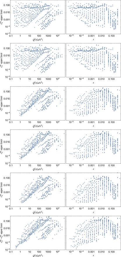
Figure 3: Estimated 95% C.L. constraints on magnitudes of $c_{u}^{\mu\nu}$ from each HERA data point.

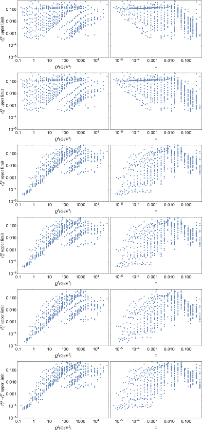
Figure 4: Estimated 95% C.L. constraints on magnitudes of $c_{d}^{\mu\nu}$ from each HERA data point.

For simplicity and following accepted procedure [6], we study in turn each of the 12 relevant components of $c_{f}^{\mu\nu}$, setting the others to zero. To explore the potential sensitivity attainable to studies of sidereal-time variations, we use the reported HERA value and experimental uncertainty for each measured differential cross section [7], as follows. For each measurement, we integrate the cross section (91) into four equal-sized bins in sidereal time, defined starting at $T_{\oplus}=0$. At fixed $x$ and $Q^{2}$, the integrated cross section depends on $\sigma_{\rm SM}(x,Q^{2})$ and the chosen component of $c_{f}^{\mu\nu}$. For each $x$ and $Q^{2}$, we construct a set of 1000 randomized pseudoexperiments, each with mean cross section equal to the reported value and with statistical error per bin equal to the reported experimental uncertainty scaled by the square root of the number of bins. For each pseudoexperiment, we construct a $\chi^{2}$ distribution involving four binned measurements and the two fit variables $\sigma_{\rm SM}(x,Q^{2})$ and $c^{\mu\nu}_{f}$, and we extract the 95% upper bound on the chosen component of $|c^{\mu\nu}_{f}|$. The estimated constraint on the component is then taken as the median of the upper bounds over all pseudoexperiments.

Coefficient	Individual	Combined
$|c^{TX}_{u}|$	$<4\times 10^{-5}$	$<1\times 10^{-5}$
$|c^{TY}_{u}|$	$<4\times 10^{-5}$	$<1\times 10^{-5}$
$|c^{XZ}_{u}|$	$<4\times 10^{-5}$	$<5\times 10^{-6}$
$|c^{YZ}_{u}|$	$<4\times 10^{-5}$	$<5\times 10^{-6}$
$|c^{XY}_{u}|$	$<4\times 10^{-5}$	$<3\times 10^{-6}$
$|c^{XX}_{u}-c^{YY}_{u}|$	$<1\times 10^{-5}$	$<8\times 10^{-6}$
$|c^{TX}_{d}|$	$<3\times 10^{-4}$	$<1\times 10^{-4}$
$|c^{TY}_{d}|$	$<3\times 10^{-4}$	$<1\times 10^{-4}$
$|c^{XZ}_{d}|$	$<4\times 10^{-5}$	$<2\times 10^{-5}$
$|c^{YZ}_{d}|$	$<4\times 10^{-5}$	$<2\times 10^{-5}$
$|c^{XY}_{d}|$	$<2\times 10^{-5}$	$<1\times 10^{-5}$
$|c^{XX}_{d}-c^{YY}_{d}|$	$<5\times 10^{-5}$	$<3\times 10^{-5}$

Table 1: Best estimated 95% C.L. constraints on magnitudes of $c_{u}^{\mu\nu}$ and $c_{d}^{\mu\nu}$.

The results of this analysis for each of the relevant components of $c^{\mu\nu}_{u}$ and $c^{\mu\nu}_{d}$ are presented in Figs. 3 and 4, respectively. Each panel shows the expected upper bound as a function of $Q^{2}$ (left) and $x$ (right). Each point is constructed from one of the 644 neutral-current HERA measurements [7]. The strongest individual constraints come mostly from measurements at low $x$ and low $Q^{2}$, close to the kinematical boundary $Q^{2}=sx$, and they are summarized in Table 1. By construction, the constraints we find are two-sided and symmetric. Note that in a real analysis, more bins could help refine the study of the second harmonics. Also, the DIS cross sections for H1 and ZEUS are distinct due to the different rotations (90), so the two detectors have different sensitivities to Lorentz violation. However, as the beam directions at the two detectors are opposite, keeping only one coefficient component at a time implies that the two cross sections are related by a parity transformation, and they therefore reduce to equivalent forms for the present analysis.

Finally, we perform a global sidereal-time analysis of the whole HERA dataset, combining all measurements into a single $\chi^{2}$ distribution. The estimated constraints obtained via this procedure are also listed in Table 1. They are stronger than the best single-measurement constraints because the global analysis takes full advantage of correlations between the binned integrated cross sections at different values of $x$ and $Q^{2}$.

To summarize, in this work we obtained expressions for the Lorentz-violating differential cross section for DIS of electrons on protons. We showed that data taken at HERA have the potential to place first constraints on certain types of Lorentz violation in the quark sector by searching for oscillations of the measured cross section at harmonics of the Earth’s sidereal frequency. Our estimates reveal a potential sensitivity of parts in a million could be attained to certain dimensionless quark coefficients $c_{f}^{\mu\nu}$ for Lorentz violation.

Related studies could also be performed for DIS data for proton-antiproton interactions in the Tevatron collider at Fermilab and for proton-proton interactions in the Large Hadron Collider at CERN. Incorporating spin dependence in the theory could also reveal sensitivity to other coefficients and open the possibility of experimental constraints from polarized DIS, potentially also including muon-sector effects. Extending the analysis to include Lorentz violation in the sea could allow first constraints on certain gluon coefficients and other quark flavors. The prospects for future direct investigations of quark-sector Lorentz violation are excellent.

References

• [1] E.D. Bloom et al., Phys. Rev. Lett. 23, 930 (1969); M. Breidenbach et al., Phys. Rev. Lett. 23, 935 (1969).
• [2] J.D. Bjorken, Phys. Rev. 179, 1547 (1969).
• [3] R.P. Feynman, Phys. Rev. Lett. 23, 1415 (1969).
• [4] See, for example, Proceedings of the 24th International Workshop on Deep Inelastic Scattering, POS DIS2016 (2016).
• [5] V.A. Kostelecký and S. Samuel, Phys. Rev. D 39, 683 (1989); V.A. Kostelecký and R. Potting, Nucl. Phys. B 359, 545 (1991); Phys. Rev. D 51, 3923 (1995).
• [6] Data Tables for Lorentz and CPT Violation, V.A. Kostelecký and N. Russell, Rev. Mod. Phys. 83, 11 (2011); 2017 edition arXiv:0801.0287v10.
• [7] H. Abramowicz et al., Eur. Phys. J. C 75, 580 (2015).
• [8] See, for example, S. Weinberg, Proc. Sci. CD 09, 001 (2009).
• [9] D. Colladay and V.A. Kostelecký, Phys. Rev. D 55, 6760 (1997); Phys. Rev. D 58, 116002 (1998).
• [10] V.A. Kostelecký, Phys. Rev. D 69, 105009 (2004).
• [11] O.W. Greenberg, Phys. Rev. Lett. 89, 231602 (2002).
• [12] For reviews see, for example, J.D. Tasson, Rep. Prog. Phys. 77, 062901 (2014); R. Bluhm, Lect. Notes Phys. 702, 191 (2006).
• [13] V.A. Kostelecký, Phys. Rev. Lett. 80, 1818 (1998).
• [14] D. Babusci et al., Phys. Lett. B 730, 89 (2014); H. Nguyen, hep-ex/0112046; V.A. Kostelecký, Phys. Rev. D 61, 016002 (1999).
• [15] K.R. Schubert, arXiv:1607.05882; R. Aaij et al., Phys. Rev. Lett. 116, 241601 (2016); V.M. Abazov et al., Phys. Rev. Lett. 115 161601 (2015); V.A. Kostelecký and R.J. Van Kooten, Phys. Rev. D 82, 101702(R) (2010); B. Aubert et al., Phys. Rev. Lett. 100, 131802 (2008); J. Link et al., Phys. Lett. B 556, 7 (2003); V.A. Kostelecký, Phys. Rev. D 64, 076001 (2001).
• [16] V.M. Abazov et al., Phys. Rev. Lett. 108, 261603 (2012).
• [17] M.S. Berger, V.A. Kostelecký, and Z. Liu, Phys. Rev. D 93, 036005 (2016).
• [18] O. Gagnon and G.D. Moore, Phys. Rev. D 70, 065002 (2004); V.A. Kostelecký and M. Mewes, Phys. Rev. D 88, 096006 (2013).
• [19] R. Kamand, B. Altschul, and M.R. Schindler, Phys. Rev. D 95, 056005 (2017); J.P. Noordmans, J. de Vries, and R.G.E. Timmermans, Phys. Rev. C 94, 025502 (2016).
• [20] V.A. Kostelecký, Phys. Lett. B 701, 137 (2011).
• [21] Y. Bonder, Phys. Rev. D 91, 125002 (2015); V.A. Kostelecký and J.D. Tasson, Phys. Rev. D 83, 016013 (2011); V.A. Kostelecký and N. Russell, Phys. Lett. B 693, 443 (2010); B. Altschul, J. Phys. A 39 13757 (2006); R. Lehnert, Phys. Rev. D 74, 125001 (2006); Q.G. Bailey and V.A. Kostelecký, Phys. Rev. D 70, 076006 (2004); D. Colladay and P. McDonald, J. Math. Phys. 43, 3554 (2002); V.A. Kostelecký and R. Lehnert, Phys. Rev. D 63, 065008 (2001).
• [22] D. Colladay and V.A. Kostelecký, Phys. Lett. B 511, 209 (2001).
• [23] M.E. Peskin and D.V. Schroeder, An Introduction to Quantum Field Theory, Perseus, Reading, Massachussetts, 1995.
• [24] D. Colladay and P. McDonald, Phys. Rev. D 77, 085006 (2008); V.A. Kostelecký, C.D. Lane, and A.G.M. Pickering, Phys. Rev. D 65, 056006 (2002).
• [25] C.G. Callan, Jr. and D.J. Gross, Phys. Rev. Lett. 21, 311 (1968).
• [26] V.A. Kostelecký and M. Mewes, Phys. Rev. D 66, 056005 (2002); R. Bluhm et al., Phys. Rev. D 68, 125008 (2003); Phys. Rev. Lett. 88, 090801 (2002).
• [27] V.A. Kostelecký, A.C. Melissinos, and M. Mewes, Phys. Lett. B 761, 1 (2016); Y. Ding and V.A. Kostelecký, Phys. Rev. D 94, 056008 (2016).
• [28] K.A. Olive et al., Chin. Phys. C 38, 090001 (2014).
• [29] E. Godat, arXiv:1510.06009.
• [30] D.B. Clark, E. Godat, and F.I. Olness, arXiv:1605.08012.
• [31] H.L. Lai et al., Phys. Rev. D 82, 074024 (2010).