Fluctuation-induced modifications of the phase structure in $(2\!+\!1)$-flavor QCD

Abstract

The low-energy sector of QCD with $N_{f}=2\!+\!1$ dynamical quark flavors at non-vanishing chemical potential and temperature is studied with a non-perturbative functional renormalization group method. The analysis is performed in different truncations in order to explore fluctuation-induced modifications of the quark-meson correlations as well as quark and meson propagators on the chiral phase transition of QCD. Depending on the chosen truncation significant quantitative implications on the phase transition are found. In the chirally symmetric phase, the quark flavor composition of the pseudoscalar $(\eta,\eta^{\prime})$-meson complex turns out to be drastically sensitive to fluctuation-induced modifications in the presence of the axial $U(1)_{A}$ anomaly. This has important phenomenological consequences for the assignment of chiral partners to these mesons.

I Introduction

The phase structure of QCD remains to be one of the most important yet unresolved problems of heavy-ion physics. Owing in particular to lattice gauge theory simulations, the region of very small density seems to be well understood. A crossover transition from a confined phase with explicitly and spontaneously broken chiral symmetry around the pseudocritical temperature $T_{c}\!\approx\!155\,\text{MeV}$ to the quark-gluon plasma phase takes place at vanishing quark chemical potential Aoki et al. (2006); Borsanyi et al. (2010); Petreczky (2012). However, the notorious sign problem renders lattice simulations unreliable at larger densities. While much progress in circumventing the sign problem has been made in recent years, see e.g. Aarts (2016), a full resolution in the near future is highly unlikely. However, present and future heavy-ion collider experiments such as the Beam Energy Scan at RHIC Adamczyk et al. (2014a, b), the NA61/SHINE experiment at the SPS at CERN Gazdzicki et al. (2006) or the CBM experiment at FAIR Friman et al. (2011) as well as NICA at JINR Kekelidze et al. (2012) start to investigate also the large density region of QCD. It is therefore indispensable to develop reliable descriptions of QCD at finite density.

Functional continuum methods such as the functional renormalization group (FRG) Braun et al. (2011); Mitter et al. (2015); Cyrol et al. (2016) or Dyson-Schwinger equations (DSE) Alkofer and von Smekal (2001); Fischer (2006); Fischer et al. (2014a) provide powerful non-perturbative tools to describe QCD from first principles also at finite density. In both cases, a solution of QCD corresponds to the solution of an infinite tower of coupled partial differential equations. In order to reduce the system to a manageable size, truncation schemes have to be devised. Systematic extensions of a given truncation allow for systematic error estimates and can be utilized to identify quantitatively precise approximation schemes.

One of the biggest challenges is to capture the drastic change of relevant degrees of freedom at the phase boundary. While quarks and gluons are the relevant objects above $T_{c}$, hadrons determine the system for low temperatures. Owing to asymptotic freedom the underlying idea is that a rising gauge coupling towards lower scales generates effective four-quark (and higher) interactions. At the scale of chiral symmetry breaking, these interactions develop poles in the corresponding quark-antiquark scattering channels which signals the formation of mesonic bound states. At lower energy scales they then become the dominant degrees of freedom. Within the FRG a practical description of this dynamical transition from quarks and gluons to hadrons is provided by dynamical hadronization, see Gies and Wetterich (2002, 2004); Pawlowski (2007); Floerchinger and Wetterich (2009); Braun et al. (2016) and Braun (2009); Mitter et al. (2015); Braun et al. (2016); Rennecke (2015a) for explicit QCD applications. Here we restrict ourselves to the low-energy sector and assume that the gauge sector is fully integrated out at these scales. How such quark-meson-type models emerge dynamically in the low-energy sector of QCD under these assumptions is well understood and explained e.g. in Schaefer and Wambach (2008); Braun et al. (2011); Kondo (2010); Herbst et al. (2011, 2013); Haas et al. (2013); Herbst et al. (2014); Mitter et al. (2015); Braun et al. (2016). However, the precise scale of the gluon decoupling is still under debate which we will pick up in Sec. IV.1. For the present purpose, it is sufficient to assume the decoupling of the gluons below a certain UV scale $\Lambda$.

In the present work, we concentrate on the hadronic low-energy sector of QCD with $N_{f}=2+1$ dynamical quark flavors at finite temperature and chemical potential. Our main question is how quark and meson fluctuations influence the chiral phase boundary, cf. e.g. Schaefer (2012). This allows us to gain valuable insights into the impact of these fluctuation on the critical endpoint (CEP) as well as the physics in the vicinity of the chiral phase boundary. The axial $U(1)_{A}$ anomaly as well as mesonic self-interactions in terms of the full effective meson potential have been investigated with the FRG in Mitter and Schaefer (2014). It was shown that fluctuation-induced effects beyond mean-field significantly weaken the chiral phase transition compared to standard mean-field studies such that the CEP is moved to small temperature and large chemical potential. In addition, the location of the CEP also strongly depends on the presence of the axial anomaly when meson fluctuations are taken into account. In Mitter and Schaefer (2014) quarks and mesons have been assumed to obey their classical dispersion relations, i.e., the propagators have the classical momentum dependence and quantum corrections to quark-meson correlations have been neglected. However, fluctuation-induced corrections to both the dispersion relations and quark-meson correlations can have a significant impact on the chiral phase boundary as found recently for low-energy QCD with two flavors Pawlowski and Rennecke (2014) and play a crucial role in the transition from the quark-gluon to the hadronic regime in two-flavor QCD Braun et al. (2016); Rennecke (2015a). This motivates us to include these corrections of the low-energy sector of $(2+1)$-flavor QCD in the present study by allowing for running quark and meson wave function renormalizations as well as running quark-meson Yukawa couplings. In this way we substantially extend our previous works in Mitter and Schaefer (2014); Pawlowski and Rennecke (2014).

Phenomenologically, chiral symmetry breaking manifests itself in the absence of parity-doublets in the experimentally observed spectrum of low-mass mesons. On the other hand, chiral symmetry restoration is signaled by the degeneration of the masses of chiral partners. In addition to the total and orbital angular momentum, also the quark composition determines which mesons eventually form chiral partners if chiral symmetry is restored. In particular the quark composition of mesons which cannot be described as simple flavor-eigenstates, can potentially be intricate. A relevant example is the pseudoscalar $\eta$- and $\eta^{\prime}$-meson complex, whose quark composition is described by the pseudoscalar mixing angle $\varphi_{p}$. This angle depends on the microscopic details of the theory as well as on temperature and density. This dependence has been studied within Nambu–Jona-Lasinio, linear sigma and quark-meson models mostly in mean-field approximation Lenaghan et al. (2000); Costa et al. (2005); Schaefer and Wagner (2009); Tiwari (2013); Kovacs et al. (2016). Here, we go beyond such approximations and study the impact of quark and meson fluctuations on the mixing angles at finite temperature and density.

The paper is organized as follows: We develop a low-energy model for the hadronic sector of 2+1-flavor QCD, which includes the above discussed effects in Sec. II. In the following Section III the incorporation of non-perturbative quantum and thermal fluctuation by means of the functional renormalization group is depicted. The corresponding flow equations for the effective potential, wave function renormalization as well as Yukawa couplings are derived in detail. Our results are presented in Sec. IV. After discussing the initial conditions for the flow equations, we first compare the chiral phase structure including a critical endpoint in different truncations. A brief discussion on related systematic errors will be given in Sec. IV.2. The quark composition of scalar and pseudoscalar mesons and its relation to the axial anomaly is addressed. We summarize our results and give an outlook in Sec. V. Computational details are provided in the four appendices.

II Effective Model for $N_{f}=2+1$ QCD at Low Energies

As argued in the introduction the low-energy sector of $N_{f}=2+1$ quark flavor QCD can be described by a linear sigma model with dynamical (constituent) quarks also known as a quark-meson model. As explained in more detail in Sec. III.1, we include quantum fluctuations by means of the FRG. Since quantum effects in this approach are driven by off-shell fluctuations of the fields, the lightest mesons give rise to the dominant quantum corrections. The dynamics of low-energy QCD are captured decisively by the inclusion of the pseudoscalar meson nonets and chiral symmetry requires the inclusion of the scalar meson nonet. Hence, we consider the lightest scalar and pseudoscalar meson nonets and the three lightest (constituent) quarks $u$, $d$ and $s$. A simplified variant of the resulting effective model setup has been studied in Mitter and Schaefer (2014). Here, we go beyond this work by allowing for fluctuation-induced corrections to the classical dispersion relations of quarks and mesons as well as to quark-meson scattering for the first time.

This leads us to the RG scale-dependent effective action

$$\begin{split}\Gamma_{k}&=\int_{x}\biggl{\{}i\bar{q}Z_{q,k}\bigl{(}\gamma_{\mu}\partial_{\mu}+\gamma_{0}\mu\bigr{)}\,q+i\bar{q}\,h_{q,k}\!\cdot\!\Sigma_{5}q\\ &\quad+\mathrm{tr}\,\bigl{(}\!Z_{\Sigma,k}\partial_{\mu}\Sigma\!\cdot\!\partial_{\mu}\Sigma^{\dagger}\bigr{)}+\tilde{U}_{k}(\Sigma,\Sigma^{\dagger})\biggr{\}}\,,\end{split}$$ (1)

with the flavor independent quark chemical potential $\mu$ and the finite temperature $T$ introduced via the Matsubara formalism such that the integral reads $\int_{x}=\int_{0}^{1/T}\!dx_{0}\int\!d^{3}x$. We assume isospin symmetry in the light quark flavor sector and label the quark fields by $q=(l,l,s)$ with the light quarks $l\equiv u=d$ and the strange quark $s$. As denoted, all parameters depend on the RG scale $k$. The quark wave function renormalization $Z_{q,k}$ encodes the fluctuation-induced modifications of the dispersion relation of the quark. The running Yukawa coupling $h_{q,k}$ couples mesons to quark-antiquark pairs. Both $Z_{q,k}$ and $h_{q,k}$ are matrices in flavor space and read for the isospin symmetric theory,

$$Z_{q,k}=\begin{pmatrix}Z_{l,k}&0&0\\ 0&Z_{l,k}&0\\ 0&0&Z_{s,k}\end{pmatrix}\,,\quad h_{q,k}=\begin{pmatrix}h_{l,k}&h_{l,k}&h_{ls,k}\\ h_{l,k}&h_{l,k}&h_{ls,k}\\ h_{sl,k}&h_{sl,k}&h_{s,k}\end{pmatrix}\,.$$ (2)

The meson field $\Sigma$ includes the scalar and pseudoscalar mesons $\sigma_{a}$ and $\pi_{a}$ in the adjoint representation of $U(N_{f})$,

$$\Sigma=T_{a}(\sigma_{a}+i\pi_{a})\,,\quad a=0,\ldots,8$$ (3)

where $T_{1},\dots,T_{N_{f}^{2}-1}$ are the generators of $SU(N_{f})$ and $T_{0}=\frac{1}{\sqrt{2N_{f}}}\mathds{1}_{N_{f}\times N_{f}}$. For $N_{f}=3$ the generators are given by the usual Gell-Mann matrices $\lambda_{a}=2T_{a}$. Additionally, the $\Sigma_{5}$ field couples to the quarks in a chirally symmetric manner and reads

$$\Sigma_{5}=T_{a}(\sigma_{a}+i\gamma_{5}\pi_{a})\,.$$ (4)

The meson effective potential $\tilde{U}_{k}(\Sigma,\Sigma^{\dagger})$ in (1) encodes all momentum-independent mesonic correlation functions. It can be decomposed into a chirally symmetric part and various contributions that break subgroups of the underlying $U(3)\!\times\!U(3)$ chiral symmetry. The chirally invariant part of this potential has to be a function of the $U(3)\!\times\!U(3)$ invariants $\rho_{1}$ and $\tilde{\rho}_{2}$, which are defined as

$$\begin{split}\rho_{1}&=\mathrm{tr}\,\left(\Sigma\!\cdot\!\Sigma^{\dagger}\right)\,,\\ \tilde{\rho}_{2}&=\mathrm{tr}\,\Bigl{(}\!\Sigma\!\cdot\!\Sigma^{\dagger}-\frac{1}{2}\rho_{1}\mathds{1}_{3\times 3}\Bigr{)}^{2}\,.\end{split}$$ (5)

In general, $\tilde{U}_{k}$ could additionally depend on the third chiral invariant $\tilde{\rho}_{3}=\mathrm{tr}\,(\Sigma\cdot\Sigma^{\dagger}-\frac{1}{2}\rho_{1}\mathds{1}_{3\times 3})^{3}$, which we drop here for the sake of simplicity. In order to capture the anomalous breaking of the axial $U(1)_{A}$ symmetry, i.e. the axial anomaly, we furthermore introduce the instanton induced Kobayashi-Maskawa-’t Hooft (KMT) determinant Kobayashi and Maskawa (1970); ’t Hooft (1976a, b),

$$\xi={\rm det}\,(\Sigma+\Sigma^{\dagger})\,,$$ (6)

to the potential, which constitues the lowest-order of a $U(1)_{A}$-symmetry breaking operator. The non-vanishing masses of the Goldstone bosons, which are directly linked to the finite current quark masses, are incorporated by an explicit chiral symmetry breaking via

$$\mathrm{tr}\,\bigl{[}\!T_{a}j_{a}(\Sigma+\Sigma^{\dagger})\bigr{]}=j_{a}\sigma_{a}\,.$$ (7)

Due to the spontaneous chiral symmetry breaking in the vacuum, a finite vacuum expectation value (VEV) of the $\Sigma$ field is generated which should carry the quantum numbers of the vacuum. This results in only non-vanishing explicit symmetry breaking parameters that correspond to the diagonal $U(3)$-generators $T_{0},T_{3}$ and $T_{8}$. Otherwise, unphysical charged chiral condensates would be generated. For the assumed light isospin symmetry this yields $j_{0},j_{8}\neq 0$ and $j_{3}=0$. Consequently, only the scalar fields $\sigma_{0}$ and $\sigma_{8}$ assume non-vanishing VEVs which are determined by minimization of the effective potential.

In summary, the effective potential has the following structure

$$\tilde{U}_{k}(\Sigma,\Sigma^{\dagger})=U_{k}(\rho_{1},\tilde{\rho}_{2})-c_{k}\xi-j_{L}\sigma_{L}-j_{S}\sigma_{S}\,,$$ (8)

wherein the chirally symmetric part of the potential, $U_{k}(\rho_{1},\tilde{\rho}_{2})$, is still an arbitrary function of the chiral invariants $\rho_{1}$ and $\tilde{\rho}_{2}$. In practice, we will compute it numerically by using the two-dimensional generalization of the fixed background Taylor expansion that was put forward in Pawlowski and Rennecke (2014). A detailed discussion of the numerical implementation can be found in App. A. Note that we have expressed the explicit symmetry breaking terms in Eq. (8) in the light-strange (LS) basis as explained below.

The explicit symmetry breaking terms $j_{L/S}$ are directly related to the quark masses $m_{q,k}$ via

$$j_{L}=\frac{2\nu_{L,k}}{h_{l,k}}m_{l,k}\,,\qquad j_{S}=\frac{\sqrt{2}\nu_{S,k}}{h_{s,k}}m_{s,k}\,,$$ (9)

with the coefficients $\nu_{L/S,k}=\sigma_{L/S}^{-1}\partial_{\sigma_{L/S}}(U_{k}-c_{k}\xi)$, where the expression inside the bracket is evaluated at the minimum of $\tilde{U}_{k}$. Without loss of generality, we choose $j_{L/S}$ to be $k$-independent. The quark masses themselves are related to the mesonic VEVs and the Yukawa couplings by

$$m_{l,k}=\frac{h_{l,k}}{2}\sigma_{L}\,,\qquad m_{s,k}=\frac{h_{s,k}}{\sqrt{2}}\sigma_{S}\,.$$ (10)

The (bare) pion and kaon decay constants $f_{\pi}$ and $f_{K}$ are related to the mesonic VEVs by Lenaghan et al. (2000)

$$f_{\pi}=\sigma_{L}\,,\qquad f_{K}=\frac{\sigma_{L}+\sqrt{2}\sigma_{S}}{2}\,.$$ (11)

Later, the mesonic VEVs become also $k$-dependent which we suppress here. In terms of the physical scalar and pseudoscalar meson fields, $\Sigma$ reads

$$\Sigma=\frac{1}{\sqrt{2}}\begin{pmatrix}\frac{1}{\sqrt{2}}\left(\sigma_{L}+a_{0}^{0}+i\eta_{L}+i\pi^{0}\right)&a_{0}^{-}+i\pi^{-}&\kappa^{-}+iK^{-}\\ a_{0}^{+}+i\pi^{+}&\frac{1}{\sqrt{2}}\left(\sigma_{L}-a_{0}^{0}+i\eta_{L}-i\pi^{0}\right)&\kappa^{0}+iK^{0}\\ \kappa^{+}+iK^{+}&\bar{\kappa}^{0}+i\bar{K}^{0}&\frac{1}{\sqrt{2}}\left(\sigma_{S}+i\eta_{S}\right)\end{pmatrix}\,,$$ (12)

where we have employed the light-nonstrange–strange (LS) basis, in which the original scalar $\sigma$ (pseudoscalar $\eta$) fields decompose into mesons made of only light-nonstrange quarks $\sigma_{L},\,\eta_{L}$ and strange quarks $\sigma_{S},\,\eta_{S}$ respectively. Hence, they are flavor eigenstates. The physical states are the mass eigenstates which are obtained from diagonalizing the Hessian $H_{ij}=\partial_{\phi_{i}}\partial_{\phi_{j}}\tilde{U}(\Sigma,\Sigma^{\dagger})$, where the fields $\phi_{i}$ comprises all physical mesons in the LS basis as in Eq. (12). Note that there are no two-point functions that mix scalar and pseudoscalar fields. Thus, $H_{ij}$ assumes a block-diagonal form with one scalar and one pseudoscalar block. The off-diagonal elements in each block are the $\sigma_{L},\sigma_{S}$ and $\eta_{L},\eta_{S}$ entries. Since the Hessian is furthermore symmetric, we can diagonalize it by introducing the scalar and pseudoscalar mixing angles $\varphi_{s}$ and $\varphi_{p}$ which rotate the LS-fields into the known physical states

$$\begin{split}\begin{pmatrix}f_{0}\\ \sigma\end{pmatrix}&=\begin{pmatrix}\cos\varphi_{s}&-\sin\varphi_{s}\\ \sin\varphi_{s}&\cos\varphi_{s}\end{pmatrix}\begin{pmatrix}\sigma_{L}\\ \sigma_{S}\end{pmatrix}\,,\\ \begin{pmatrix}\eta\\ \eta^{\prime}\end{pmatrix}&=\begin{pmatrix}\cos\varphi_{p}&-\sin\varphi_{p}\\ \sin\varphi_{p}&\cos\varphi_{p}\end{pmatrix}\begin{pmatrix}\eta_{L}\\ \eta_{S}\end{pmatrix}\,.\end{split}$$ (13)

All other fields in Eq. (12) are already mass eigenstates.

Furthermore, the fields in the singlet-octet (08) basis as used in Eq. (3) can be transformed into the LS basis by

$$\begin{pmatrix}\phi_{L}\\ \phi_{S}\end{pmatrix}=\frac{1}{\sqrt{3}}\begin{pmatrix}1&\sqrt{2}\\ -\sqrt{2}&1\end{pmatrix}\begin{pmatrix}\phi_{8}\\ \phi_{0}\end{pmatrix}\,.$$ (14)

For more details on the mixing angles we defer to App. C. In summary, the vector of all physical mesons then is

$$\begin{split}\phi=(&f_{0},a_{0}^{0},a_{0}^{+},a_{0}^{-},\kappa^{+},\kappa^{-},\kappa^{0},\bar{\kappa}^{0},\sigma,\\ &\eta,\pi^{0},\pi^{+},\pi^{-},K^{+},K^{-},K^{0},\bar{K}^{0},\eta^{\prime})\,.\end{split}$$ (15)

In the present isospin symmetric setup only the $f_{0}$ and $\sigma$ assume a non-vanishing vacuum expectation value. These are directly linked to the light and strange quark condensates which are, in turn, related to the vacuum expectation values of $\sigma_{L}$ and $\sigma_{S}$. We therefore conveniently define the VEV of $\phi$ as

$$\phi_{0}\equiv(\sigma_{L},\sigma_{S},0,\ldots,0)\,.$$ (16)

III Fluctuations

As already mentioned the present work aims at fluctuation-induced effects in the low-energy sector of QCD which are particularly relevant in the vicinity of the chiral phase transition where long-range correlations occur. In the FRG framework quantum fluctuations result in a running of all parameters of the effective average action $\Gamma_{k}$ in Eq. (1). In the following, we will give a brief outline of the used FRG to incorporate fluctuations here. This is followed by a discussion on the corresponding beta functions, or flow equations of the parameters of our truncation. For reviews of the FRG we refer the reader to Berges et al. (2002); Pawlowski (2007); Gies (2012); Schaefer and Wambach (2008); Delamotte (2012); Rosten (2012); Braun (2012).

III.1 The Functional Renormalization Group

The underlying idea of K. G. Wilson’s version of the renormalization group is to integrate out quantum fluctuations successively . In the present case, one begins with the microscopic action $\Gamma_{k=\Lambda}$ at some large initial momentum scale $\Lambda$ in the ultraviolet (UV). By lowering the RG scale $k$, quantum fluctuations are successively integrated out until one arrives at the full macroscopic quantum effective action $\Gamma\equiv\Gamma_{k=0}$ at $k=0$. Ideally, one starts in the perturbative regime where the initial effective action $\Gamma_{k=\Lambda}$ is given by the well-known microscopic action of QCD. In our truncation we assume that gluon degrees of freedom are already integrated out which fixes the initial scale by the scale of the gluon decoupling and is therefore directly linked to the gluon mass gap. Based on results in Landau gauge QCD Fischer et al. (2009); Maas (2013), this yields UV scale choices of the order $\Lambda\lesssim 1\,\text{GeV}$.

A convenient realization of Wilson’s RG idea is given in terms of a functional differential equation for the 1PI effective average action, the Wetterich equation Wetterich (1993). For the present $2+1$-flavor quark-meson model truncation with two meson nonets and two light and one strange quark flavor the evolution equation of the scale dependent effective average action $\Gamma_{k}$ reads explicitly

$$\begin{split}\partial_{t}\Gamma_{k}&=\frac{1}{2}\sum_{i=1}^{2N_{f}^{2}}\mathrm{Tr}\left(\!G_{\phi_{i},k}\!\cdot\partial_{t}R_{k}^{\phi_{i}}\right)\\ &\quad-2\mathrm{Tr}\left(G_{l,k}\!\cdot\partial_{t}R_{k}^{l}\right)-\mathrm{Tr}\left(G_{s,k}\!\cdot\partial_{t}R_{k}^{s}\right)\,,\end{split}$$ (17)

where $\partial_{t}=k\frac{d}{dk}$ denotes the logarithmic scale derivative. The trace runs over all discrete and continuous indices, i.e. color, spinor and the loop momenta and/or frequencies respectively. The sum in the first line is over all $2N_{f}^{2}$ scalar and pseudoscalar mesons, cf. Eq. (15). $G_{\phi_{i},k}$ denotes the generalized meson and quark propagators

$$\begin{split}G_{\phi_{i},k}[\Phi]&=\left(\frac{\delta^{2}\Gamma_{k}[\Phi]}{\delta\phi_{i}(-p)\delta\phi_{i}(p)}+R_{k}^{\phi_{i}}\right)^{-1}\,,\\ G_{q,k}[\Phi]&=\left(\frac{\delta^{2}\Gamma_{k}[\Phi]}{\delta q(-p)\delta\bar{q}(p)}+R_{k}^{q}\right)^{-1}\,,\end{split}$$ (18)

with the super field $\Phi=(\phi,q,\bar{q})$. Evaluated on the equations of motion at $k=0$, i.e., on the vacuum expectation value $\Phi_{0}=(\phi_{0},0,0)$, these generalized propagators reduce to the full propagators. The scale-dependent IR regulators $R_{k}^{\phi_{i}}$ can be understood as momentum-dependent squared masses that suppress the infrared modes of the field $\phi_{i}$. In addition, the terms $\partial_{t}R_{k}^{\phi_{i}}$ in Eq. (17) also ensure UV-regularity. Their definitions (see Eq. (50)) and further details are collected in App. B.

Inserting the truncation for the effective average action $\Gamma_{k}$ in Eq. (1) in the flow equation (17) yields a closed set of coupled differential equations for all scale-dependent parameters of $\Gamma_{k}$. Note that the physical parameters are RG-scale dependent but invariant under general reparameterizations. In the present case, this is achieved by an appropriate rescaling with the wave function renormalizations. The physical quark and meson masses are then given by

$$M_{q,k}=\frac{m_{q,k}}{Z_{q,k}}\,,\qquad M_{\phi_{i},k}=\frac{m_{\phi_{i},k}}{Z_{\phi_{i},k}^{1/2}}\,,$$ (19)

where the meson masses $m_{\phi_{i},k}$ are the eigenvalues of the Hessian of the effective potential. The explicit expressions are given in App. D.

For simplicity, however, we assume that all mesons have the same anomalous dimension $Z_{\phi,k}\equiv Z_{\phi_{i},k}$, i.e., we choose $Z_{\Sigma,k}=\text{diag}\,(Z_{\phi,k},\,Z_{\phi,k},\,Z_{\phi,k})$ in Eq. (1). Accordingly, the scale-dependent physical VEV of the fields is given by

$$\bar{\phi}_{0}=(\bar{\sigma}_{L},\bar{\sigma}_{S},0,\ldots,0)=Z_{\phi,k}^{1/2}\phi_{0}\,,$$ (20)

where the index $k$ on the VEV’s has been suppressed. In the following we will use the bar notation over a coupling to denote its rescaling with the wave function renormalization. The running Yukawa coupling is

$$\bar{h}_{q,k}=\frac{h_{q,k}}{Z_{q,k}Z_{\phi,k}^{1/2}}\,.$$ (21)

The chiral invariants and the KMT determinant are then

$$\bar{\rho}_{1}=Z_{\phi,k}\rho_{1}\,,\quad\bar{\tilde{\rho}}_{2}=Z_{\phi,k}^{2}\tilde{\rho}_{2}\,,\quad\bar{\xi}=Z_{\phi,k}^{3/2}\xi\,,$$ (22)

and the effective potential is fixed from the requirement of reparametrization invariance,

$$\bar{U}_{k}(\bar{\rho}_{1},\bar{\tilde{\rho}}_{2})=U_{k}(\rho_{1},\tilde{\rho}_{2})\,.$$ (23)

The consequence of reparametrization invariance in the present case is that the wave function renormalizations do not enter the flow equations directly, but only through the corresponding anomalous dimensions

$$\eta_{\Phi,k}=-\frac{\partial_{t}Z_{\Phi,k}}{Z_{\Phi,k}}\,.$$ (24)

Thus, introducing wave function renormalizations in this way implies that it is not necessary to solve their flow equation explicitly. One only needs to know the anomalous dimensions for the solution of the present truncation. The anomalous dimensions, in turn, can be computed analytically.

In the following, we briefly discuss the structure of the flow equations for the effective potential, Yukawa couplings and anomalous dimension.

III.2 Flow of the Effective Potential

All physical information is extracted from the effective potential evaluated at the minimum at $k=0$. The meson fields assume their vacuum expectation value at this point. As discussed above, the VEV $\phi_{0}$ has two non-vanishing components which are most conveniently expressed in the LS-basis, $\sigma_{L,k=0}$ and $\sigma_{S,k=0}$. With a slight abuse of terminology, we refer to them as the light and strange condensates . They are obtained from the simultaneous solution of

$$\begin{split}\partial_{\sigma_{L}}\tilde{U}_{k}(\Sigma,\Sigma^{\dagger})\big{|}_{\phi_{0}}=0\,,\quad\text{and}\quad\partial_{\sigma_{S}}\tilde{U}_{k}(\Sigma,\Sigma^{\dagger})\big{|}_{\phi_{0}}=0\,.\end{split}$$ (25)

The flow of the effective potential is obtained from the scale-dependent effective action for constant fields. We find for the flow of the chirally invariant part of the potential in terms of the physical fields:

$$\partial_{t}U_{k}(\rho_{1},\tilde{\rho}_{2})=$$ (26)

$$\quad\frac{k^{4}}{4\pi^{2}}\bigg{\{}l_{0}^{(B)}(\bar{m}_{f_{0},k}^{2},\eta_{\phi,k})+3l_{0}^{(B)}(\bar{m}_{a_{0},k}^{2},\eta_{\phi,k})$$

$$\quad+4l_{0}^{(B)}(\bar{m}_{\kappa,k}^{2},\eta_{\phi,k})+l_{0}^{(B)}(\bar{m}_{\sigma,k}^{2},\eta_{\phi,k})+l_{0}^{(B)}(\bar{m}_{\eta,k}^{2},\eta_{\phi,k})$$

$$\quad+3l_{0}^{(B)}(\bar{m}_{\pi,k}^{2},\eta_{\phi,k})+4l_{0}^{(B)}(\bar{m}_{K,k}^{2},\eta_{\phi,k})+l_{0}^{(B)}(\bar{m}_{\eta^{\prime},k}^{2},\eta_{\phi,k})$$

$$\quad\qquad-4N_{c}\Big{[}2l_{0}^{(F)}(\bar{m}_{l,k},\eta_{l,k})+l_{0}^{(F)}(\bar{m}_{s,k},\eta_{s,k})\Big{]}\bigg{\}}\,.$$

The last line is the contribution of the light and strange quarks to the flow. The fermion loop yields the negative sign and the particle, antiparticle with spin $1/2$ the factor four. The other lines are the contributions from the mesons. Owing to light isospin symmetry, the respective masses of the $a_{0}$-, $\kappa$-, $\pi$- and $K$-mesons degenerate and their contributions can be subsumed correspondingly into one threshold function with the respective multiplicity. The bosonic and fermionic threshold functions $l_{0}^{(B,F)}$ are functions of the dimensionless masses $\bar{m}_{\Phi,k}=M_{\Phi,k}/k$, the anomalous dimension of the corresponding field as well as temperature and chemical potential. They are defined in App. B, Eqs. (54) and (55). We cast this partial differential equation into a finite set of coupled ordinary differential equations by using the two-dimensional fixed background Taylor expansion, see App. A.

The explicit chiral symmetry breaking terms in Eq. (8) receive a canonical running after the rescaling with the wave function renormalizations discussed above. We immediately infer from $\bar{j}_{L/S}=j_{L/S}/Z_{\phi,k}^{1/2}$ and Eq. (24) that

$$\partial_{t}\bar{j}_{L/S}=\frac{1}{2}\eta_{\phi,k}\bar{j}_{L/S}\,.$$ (27)

Hence, even though explicit chiral symmetry breaking is introduced by constant source terms, reparametrization invariance results in a running of these sources.

In the case of the explicit axial symmetry breaking parameter $c_{k}$, we have to be a bit more careful. Since such a term arises originally from instanton contributions ’t Hooft (1976a), it depends in general on the scale as well as temperature and chemical potential. Determining the precise running of the axial anomaly is beyond the scope of the present work. We rather resort to an effective resolution of this issue. While the fate of the axial anomaly at temperatures close to $T_{c}$ is still under debate Cohen (1996); Birse et al. (1996); Kapusta et al. (1996); Mitter and Schaefer (2014), recent results from lattice gauge theory studies indicate that the axial symmetry is not restored for temperatures $T\lesssim 200$ MeV Bazavov et al. (2012); Buchoff et al. (2014); Sharma et al. (2014); Bhattacharya et al. (2014); Dick et al. (2015). We therefore assume a constant KMT coupling $\bar{c}=c_{k}/Z_{\phi,k}^{3/2}$, i.e.,

$$\partial_{t}\bar{c}=0\,.$$ (28)

This is equivalent to $\partial_{t}c_{k}=-\frac{3}{2}\eta_{\phi,k}c_{k}$. On the other hand, if we would require $\partial_{t}c_{k}=0$, the running anomaly strength $\bar{c}$ would increase with increasing temperature, in particular for $T\gtrsim T_{c}$. As we will see later this is because of the rapid decrease of the meson anomalous dimension with temperature in this region, cf. Fig. 4. However, $\bar{c}$ should decrease at high temperatures since instanton fluctuations are screened by the Debye mass Gross et al. (1981). Due to the finite UV cutoff the temperature independency of the initial action is also limited. For our UV cutoff choice the temperature should not exceed $T\approx 200\,\text{MeV}$ as discussed in Sec. IV.1. Hence, a constant $\bar{c}$ is a reasonable assumption which is also in accordance with numerical lattice simulations.

III.3 Running Yukawa Couplings

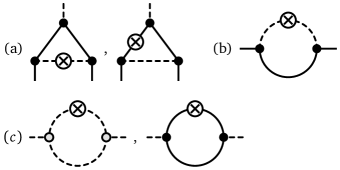
Figure 1: The different types of diagrams that contribute to the running of the Yukawa couplings (a), the quark anomalous dimensions, (b), and the meson anomalous dimensions, (c). The solid lines are the quark propagators and the dashed lines are the meson propagators. The crossed circle illustrates the insertion of the scale derivative of the regulator. The black dots denote the Yukawa couplings and the gray dots the three-meson interactions. Note that the vertices and propagators are fully dressed here and the diagram with a quark regulator insertion vanishes for the anomalous dimension.

The correlations between quarks, antiquarks and mesons, i.e., correlators of the form $\langle\bar{q}\phi q\rangle$, are incorporated by the Yukawa couplings $h_{q,k}$ given in Eq. (2). The most relevant correlation functions of this kind are those that directly contribute to the spontaneously generated constituent quark masses, Eq. (10). We will therefore concentrate on the running of the diagonal entries $h_{l,k}$ and $h_{s,k}$. This leads to a closed set of flow equations for our truncation Eq. (1) if we also restrict ourselves to meson anomalous dimensions of purely light and strange mesons. Hence, the remaining off-diagonal Yukawa couplings in Eq. (2) do not enter the system of flow equations in this case.

In Ref. Pawlowski and Rennecke (2014) it was shown that the flow of the Yukawa couplings can be extracted from the flow of the quark two-point function since they are directly related to the running of the quark masses

$$\begin{split}\partial_{t}h_{l,k}&=\frac{-i}{4N_{c}\sigma_{L}}\lim_{p\rightarrow p_{\text{ext}}}\text{Tr}\left(\frac{\delta^{2}\partial_{t}\Gamma_{k}}{\delta l(-p)\delta\bar{l}(p)}\right)\bigg{|}_{\Phi_{0}}\,,\\ \partial_{t}h_{s,k}&=\frac{-i\sqrt{2}}{4N_{c}\sigma_{S}}\lim_{p\rightarrow p_{\text{ext}}}\text{Tr}\left(\frac{\delta^{2}\partial_{t}\Gamma_{k}}{\delta s(-p)\delta\bar{s}(p)}\right)\bigg{|}_{\Phi_{0}}\,.\end{split}$$ (29)

Because the Yukawa couplings are correlation functions that carry a baryon number some caution is advised in order to fulfill the Silver Blaze property of QCD Cohen (2003). It states that at vanishing temperature, the QCD equation of state does not depend on the chemical potential as long as it is below a critical one. This directly converts to the frequency dependence of $n$-point functions with legs that carry a non-vanishing baryon number $B$. In the context of the FRG, this is discussed in detail in Khan et al. (2015) and applied in Fu and Pawlowski (2015); Fu et al. (2016). It follows that the Silver Blaze property is respected if one evaluates the flow of the correlation functions at complex frequencies $p_{0}=\tilde{p}_{0}-3iB\mu$, where $\tilde{p}_{0}$ is an arbitrary real number. As a consequence the external four-momentum $p_{\text{ext}}$ at which we evaluate correlation functions that involve quarks with baryon number $B=1/3$ are

$$p_{\text{ext}}=(p_{0,\text{ext}},\vec{p}_{\text{ext}})=(\pi T-i\mu,\vec{0})\,.$$ (30)

We have chosen the lowest fermionic Matsubara frequency for $\tilde{p}_{0,\text{ext}}=\pi T$ since quark legs in loop diagrams carry fermionic momenta. The spatial external momentum is set to zero for convenience. A diagrammatic representation of the typical contributions to the flow of the Yukawa couplings is shown in Fig. 1.

Inserting $\Gamma_{k}$ from Eq. (1) into Eq. (29) we obtain with the definition (21) the flows of the running Yukawa couplings

$$\partial_{t}\bar{h}_{l,k} =\left(\eta_{l,k}+\frac{1}{2}\eta_{\phi,k}\right)\bar{h}_{l,k}+\frac{\bar{h}_{l,k}^{3}}{4\pi^{2}}\,\bigg{(}\!\cos^{2}\!\varphi_{s}\,L_{(1,1)}^{(l,f_{0})}$$ (31)

$$\quad+L_{(1,1)}^{(l,a_{0})}+\sin^{2}\!\varphi_{s}\,L_{(1,1)}^{(l,\sigma)}-\cos^{2}\!\varphi_{p}\,L_{(1,1)}^{(l,\eta)}-L_{(1,1)}^{(l,\pi)}$$

$$\quad-\sin^{2}\!\varphi_{p}\,L_{(1,1)}^{(l,\eta^{\prime})}\bigg{)}\,,$$

for the light quark and

$$\partial_{t}\bar{h}_{s,k} =\left(\eta_{s,k}+\frac{1}{2}\eta_{\phi,k}\right)\bar{h}_{s,k}+\frac{\bar{h}_{s,k}^{3}}{4\pi^{2}}\,\bigg{(}\!\sin^{2}\!\varphi_{s}\,L_{(1,1)}^{(s,f_{0})}$$ (32)

$$\quad+\cos^{2}\!\varphi_{s}\,L_{(1,1)}^{(s,\sigma)}-\sin^{2}\!\varphi_{p}\,L_{(1,1)}^{(s,\eta)}-\cos^{2}\!\varphi_{p}\,L_{(1,1)}^{(s,\eta^{\prime})}\bigg{)}\,,$$

for the strange quark Yukawa coupling. The threshold functions for loops with internal quarks and mesons have been abbreviated by $L_{(1,1)}^{(q,\phi)}=L_{(1,1)}(\bar{m}_{q,k}^{2},\bar{m}_{\phi,k}^{2},\eta_{q,k},\eta_{\phi,k};p_{0,\text{ext}})$ and are defined in App. B, Eq. (58).

Due to the mixing of the physical $f_{0},\sigma$ and $\eta,\eta^{\prime}$ states with the corresponding purely light and strange states as defined in Eq. (13), the scalar and pseudoscalar mixing angles $\varphi_{s},\varphi_{p}$ naturally appear here. These equations couple to the flow of the effective potential through the quark masses.

III.4 Anomalous Dimensions

The wave function renormalizations encode the fluctuation-induced modifications of the corresponding fields or in other words, the deviation from the canonical momentum dependence of the propagators. In the present context, this is particularly important for the identification of Euclidean meson masses. The physical masses are defined as poles of the corresponding propagators or as roots from the inverse propagator $\bar{\Gamma}^{(2)}(p_{0},\vec{p}^{2})$ through $\bar{\Gamma}^{(2)}(im_{\text{pol}},0)=0$. In this work, we instead extract the meson masses from the curvature of the effective potential given by $\bar{\Gamma}^{(2)}(0,0)=m_{\text{cur}}^{2}$ evaluated at vanishing momenta. The computation of the pole masses would require the analytical continuation of the Euclidean two-point functions. Even though it is known how this can be achieved within the FRG Floerchinger (2012); Tripolt et al. (2014); Pawlowski and Strodthoff (2015), it is beyond the scope of the present work. However, for an effective theory setup within the FRG the difference between the pole $m_{\text{pol}}$ and curvature $m_{\text{cur}}$ masses should remain small as pointed out in Strodthoff et al. (2012). This matters because some of the physical meson masses are used as input to constrain some parameters of our effective theory.

For the utilized truncation the inverse propagator is parametrized by

$$\bar{\Gamma}^{(2)}(p_{0},\vec{p}^{2})=p_{0}^{2}+\vec{p}^{2}+\frac{m^{2}}{Z(p_{0},\vec{p}^{2})}\,,$$ (33)

which yields the relation

$$m_{\text{cur}}^{2}=\frac{Z(im_{\text{pol}},0)}{Z(0,0)}m_{\text{pol}}^{2}\,,$$ (34)

between the curvature and pole mass. Hence, the pole and curvature masses are essentially identical if the wave function renormalization only mildly depends on the (imaginary) frequency. This mild dependency has been confirmed in Helmboldt et al. (2015) for pions in a two-flavor study. In addition, the inclusion of the RG-scale dependent, but momentum-independent, wave function renormalizations $Z_{k}$ yields an agreement between the pole and curvature mass of the pion within an one percent accuracy level Helmboldt et al. (2015). Thus, by including the running wave function renormalizations, we ensure that the computed masses stay close to the physical ones which furthermore justifies our model parameter fixing based on measured masses.

Another important issue that emphasizes in particular the relevance of the meson anomalous dimension $Z_{\phi,k}$ is related to the decoupling of the mesons from the physical spectrum in the quark-gluon regime of QCD at large energies. As shown in Braun et al. (2016); Rennecke (2015a) a rapid decrease of the meson wave function renormalization drives this decoupling, see also Gies and Wetterich (2004); Braun (2009). This is also the case for three quark flavors: even without the dominating gluon fluctuations, $Z_{\phi,k}$ shows a rapid decrease for temperatures above the chiral transition, $T\!>\!T_{c}$. The resulting fast decoupling of the mesons in the chirally symmetric phase has a large impact on the phase boundary and in particular on the location of the critical endpoint as compared to previous results where this effect has been neglected Mitter and Schaefer (2014).

truncation	running couplings	$\bar{\lambda}_{10,\Lambda}$ [GeV2]	$\bar{\lambda}_{20,\Lambda}$	$\bar{\lambda}_{01,\Lambda}$	$\bar{c}$ [GeV]	$\bar{j}_{L}$ [GeV3]	$\bar{j}_{S}$ [GeV3]	$\bar{h}_{l,k}$	$\bar{h}_{s,k}$
LPA′+Y	$\bar{\tilde{U}}_{k}$, $\bar{h}_{l,k}$, $\bar{h}_{s,k}$, $Z_{l,k}$, $Z_{s,k}$, $Z_{\phi,k}$	$(1.221)^{2}$	60	210	4.808	$1.495\times(0.121)^{3}$	$1.495\times(0.336)^{3}$	9.78	9.65
LPA+Y	$\bar{\tilde{U}}_{k}$, $\bar{h}_{l,k}$, $\bar{h}_{s,k}$	$(0.836)^{2}$	7.5	50	4.808	$1\times(0.121)^{3}$	$1\times(0.336)^{3}$	5.96	6.40
LPA	$\bar{\tilde{U}}_{k}$	$(0.889)^{2}$	4.5	40	4.808	$1\times(0.121)^{3}$	$1\times(0.336)^{3}$	6.5	6.5

Table 1: Initial conditions for different truncations.

The running of the wave function renormalizations gives rise to the anomalous dimension defined in Eq. (24). For the light and strange quarks, they can be obtained from the corresponding two-point functions by

$$\begin{split}\eta_{l,k}&=-\frac{1}{16N_{c}Z_{l,k}}\lim_{p\rightarrow p_{\text{ext}}}\frac{\partial^{2}}{\partial|\vec{p}|^{2}}\text{Tr}\left(\!\vec{\gamma}\vec{p}\,\frac{\delta^{2}\partial_{t}\Gamma_{k}}{\delta l(-p)\delta\bar{l}(p)}\right)\bigg{|}_{\Phi_{0}}\,,\\ \eta_{s,k}&=-\frac{1}{8N_{c}Z_{l,k}}\lim_{p\rightarrow p_{\text{ext}}}\frac{\partial^{2}}{\partial|\vec{p}|^{2}}\text{Tr}\left(\!\vec{\gamma}\vec{p}\,\frac{\delta^{2}\partial_{t}\Gamma_{k}}{\delta s(-p)\delta\bar{s}(p)}\right)\bigg{|}_{\Phi_{0}}\,.\end{split}$$ (35)

Concerning the Silver Blaze property at vanishing temperature the same arguments as for the Yukawa coupling apply and we thus evaluate these flows at external momenta $p_{\text{ext}}$ as given in Eq. (30) which finally yields

$$\begin{split}\eta_{l,k}&=\frac{\bar{h}_{l,k}^{2}}{24\pi^{2}}(4-\eta_{\phi,k})\,\bigg{(}\!\cos^{2}\!\varphi_{s}\,\textit{FB}_{(1,2)}^{(l,f_{0})}+\textit{FB}_{(1,2)}^{(l,a_{0})}\\ &\quad+\sin^{2}\!\varphi_{s}\,\textit{FB}_{(1,2)}^{(l,\sigma)}+\cos^{2}\!\varphi_{p}\,\textit{FB}_{(1,2)}^{(l,\eta)}+\textit{FB}_{(1,2)}^{(l,\pi)}\\ &\quad+\sin^{2}\!\varphi_{p}\,\textit{FB}_{(1,2)}^{(l,\eta^{\prime})}\bigg{)}\end{split}$$ (36)

for the light and

$$\eta_{s,k} =\frac{\bar{h}_{s,k}^{2}}{24\pi^{2}}(4-\eta_{\phi,k})\,\bigg{(}\!\sin^{2}\!\varphi_{s}\,\textit{FB}_{(1,2)}^{(s,f_{0})}+\cos^{2}\!\varphi_{s}\,\textit{FB}_{(1,2)}^{(s,\sigma)}$$

$$\quad+\sin^{2}\!\varphi_{p}\,\textit{FB}_{(1,2)}^{(s,\eta)}+\cos^{2}\!\varphi_{p}\,\textit{FB}_{(1,2)}^{(s,\eta^{\prime})}\bigg{)}$$ (37)

for the strange quark anomalous dimension. For the threshold functions we have used the abbreviation $\textit{FB}_{(1,2)}^{(q,\phi)}=\textit{FB}_{(1,2)}(\bar{m}_{q,k}^{2},\bar{m}_{\phi,k}^{2},\eta_{q,k},\eta_{\phi,k};p_{0,\text{ext}})$, see App. B, Eqs. (60) and (64) for the definitions. The type of diagram that contributes to these anomalous dimensions is displayed in Fig. 1.

In Eqs. (36) and (III.4) our assumption of only one anomalous dimension $\eta_{\phi,k}$ simplifies the flow equations significantly since otherwise each meson term would have its own prefactor $(4-\eta_{\phi_{i},k})$. Of course, which of the anomalous dimension as above Eq. (20) is chosen is not unique. Since the light pions are dynamically the most relevant degrees of freedom their dynamics should be captured as accurately as possible. This motivates our choice

$$Z_{\phi,k}\equiv Z_{\pi^{+},k}\,,$$ (38)

where actually the pion charge is irrelevant due to the light isospin symmetry. The light isospin symmetry also implies the vanishing of the Yukawa couplings for the $\pi^{0}$ and for the $a_{0}^{0}$. However, this approximation could potentially lead to an overestimation of the dynamics of the heavier mesons at large temperatures. A reasonable upgrade of the present approximation would be the inclusion of further meson wave function renormalizations, e.g., a second meson wave function renormalization of a strange meson. This might be of relevance for further investigations of cumulants for strangeness number distribution. However, we will defer such an analysis to a future work.

The meson anomalous dimension defined in Eq. (38) can be extracted from the pion two-point function by

$$\eta_{\phi,k}=-\frac{1}{2Z_{\phi,k}}\lim_{p\rightarrow 0}\frac{\partial^{2}}{\partial|\vec{p}|^{2}}\text{Tr}\left(\frac{\delta^{2}\partial_{t}\Gamma_{k}}{\delta\pi^{+}(-p)\delta\pi^{+}(p)}\right)\bigg{|}_{\Phi_{0}}\,.$$ (39)

Here the Silver Blaze property is not an issue since the anomalous dimension is related to a purely mesonic correlator. We therefore set the external frequency to the lowest bosonic Matsubara mode and the external spatial momenta to zero, i.e., $p_{\text{ext}}=(0,\vec{0})$. This yields

$$\begin{split}\eta_{\phi,k}&=\frac{1}{3\pi^{2}}\bigg{[}\bar{\lambda}_{\pi^{+}\pi^{-}f_{0},k}\textit{BB}_{(2,2)}^{(\pi,f_{0})}+\bar{\lambda}_{\pi^{+}\pi^{-}\sigma,k}\textit{BB}_{(2,2)}^{(\pi,\sigma)}\\ &\quad\bar{\lambda}_{\pi^{+}a_{0}^{-}\eta,k}\textit{BB}_{(2,2)}^{(a_{0},\eta)}+\bar{\lambda}_{\pi^{+}a_{0}^{-}\eta^{\prime},k}\textit{BB}_{(2,2)}^{(a_{0},\eta^{\prime})}\\ &\quad+\big{(}\bar{\lambda}_{\pi^{+}\kappa^{-}\bar{K}^{0},k}+\bar{\lambda}_{\pi^{+}K^{-}\bar{\kappa}^{0},k}\big{)}\textit{BB}_{(2,2)}^{(K,\kappa)}\bigg{]}\\ &\quad+\frac{N_{c}\,\bar{h}_{l,k}^{2}}{6\pi^{2}}\bigg{[}4\big{(}2-\eta_{l,k}\big{)}\textit{F}_{(3)}^{\,(l)}-\big{(}3-2\eta_{l,k}\big{)}\textit{F}_{(2)}^{\,(l)}\bigg{]}\,.\end{split}$$ (40)

The involved meson three-point correlators $\bar{\lambda}_{\phi_{i}\phi_{j}\phi_{l},k}$ of the mesons $\phi_{i}$ are given in App. D. Light isospin symmetry implies $\bar{\lambda}_{\pi^{+}\kappa^{-}\bar{K}^{0},k}=\bar{\lambda}_{\pi^{+}K^{-}\bar{\kappa}^{0},k}$. The threshold functions $\textit{BB}_{(2,2)}^{(\phi_{i},\phi_{j})}=\textit{BB}_{(2,2)}(\bar{m}_{\phi_{i},k}^{2},\bar{m}_{\phi_{j},k}^{2})$ are related to purely mesonic loops but for different mesons and $\textit{F}_{(2)}^{\,(l)}=\textit{F}_{(2)}(\bar{m}_{l,k}^{2})$ corresponds to a light quark loop. The analytical expressions for these functions are given in App. B. The corresponding diagrams that contribute to the meson anomalous dimension are again shown in Fig. 1.

IV Results

IV.1 Initial Conditions

We begin with the specification of the initial effective action $\Gamma_{k=\Lambda}$ at the UV scale $\Lambda$. Within our low-energy description the initial scale $\Lambda$ is bounded on the one hand by the requirement that is has to be large enough to avoid UV-cutoff effects at large temperature and/or chemical potential and on the other hand it should be as small as possible to ensure a decoupled gauge sector. Satisfying both of these requirements is hardly possible since the gluon sector remains quantitatively relevant even at scales below the chiral transition Rennecke (2015b). We therefore choose as smallest UV-cutoff $\Lambda=900$ MeV for which cutoff effects are only minor for $T\lesssim 230\,\text{MeV}$ and $\mu\lesssim 300\,\text{MeV}$.

Furthermore, the initial effective potential $\bar{\tilde{U}}_{k=\Lambda}$ and the initial Yukawa couplings $\bar{h}_{q,k=\Lambda}$ have to be specified. For the wave function renormalizations no initial conditions have to be given explicitly since due to the reparametrization invariance of the RG-equations only the anomalous dimensions enter the flow equations. For the initial effective potential only relevant and marginal terms are chosen

$$\begin{split}\bar{\tilde{U}}_{k=\Lambda}(\bar{\rho}_{1},\bar{\tilde{\rho}}_{2})&=\bar{\lambda}_{10,k=\Lambda}\,\bar{\rho}_{1}+\frac{\bar{\lambda}_{20,k=\Lambda}}{2}\,\bar{\rho}_{1}+\bar{\lambda}_{01,k=\Lambda}\,\bar{\tilde{\rho}}_{2}\\ &\quad-\bar{c}\bar{\xi}-\bar{j}_{L}\bar{\sigma}_{L}-\bar{j}_{S}\bar{\sigma}_{S}\,,\end{split}$$ (41)

since higher-order meson correlations are generated via the flow at lower energy scales.

Together with the initial Yukawa couplings we have eight parameters to fix in the infrared. As input we use the pion and kaon decay constants, $\bar{f}_{\pi}=93\,\text{MeV}$ and $\bar{f}_{K}=114\,\text{MeV}$, the curvature masses of the pion, $M_{\pi}=138\,\text{MeV}$, the kaon, $M_{K}=492\,\text{MeV}$, the sigma meson, $M_{\sigma}=421\,\text{MeV}$ and the sum of the squared $\eta$- and $\eta^{\prime}$-masses $M_{\eta}^{2}+M_{\eta^{\prime}}^{2}=1.22\times 10^{6}\,\text{MeV}^{2}$. Furthermore, the constituent quark masses are fixed to $M_{l}=301\,\text{MeV}$ and $M_{s}=441\,\text{MeV}$.

However, these infrared conditions do not fix all initial values uniquely in the UV. This additional ambiguity can be utilized to imprint some information of the full RG flow of QCD onto our truncation. Since $\Lambda$ is chosen to be much larger than the chiral symmetry breaking scale, mesons should be already decoupled from the system and act merely as auxiliary fields. This was explicitly demonstrated for $N_{f}=2$ QCD in Braun et al. (2016); Rennecke (2015a). We implement this effectively by minimizing the meson fluctuations at large cutoff scales and require their initial masses to be larger than the cutoff scale, i.e., $M_{\phi,k=\Lambda}>\Lambda$. Since the computed curvature masses are expected to be close to the pole masses, as discussed in Sec. III.4, the condition $M_{\phi,k=\Lambda}>\Lambda$ implies that the mesons do not emerge as resonances in the corresponding spectral functions and are indeed decoupled from the physical spectrum.

To point out the physical effects of the applied effective model, we solve the flow equation system in different truncations. To fix the terminology, we denote the truncation of the effective action we introduced in Sec. III as "LPA^′+Y", i.e., we consider the full effective potential $\bar{\tilde{U}}_{k}$ together with the running Yukawa couplings discussed in Sec. III.3 as well as non-vanishing anomalous dimension as discussed in Sec. III.4. Most commonly used in the literature is the local potential approximation, "LPA", where only the scale-dependent effective potential is investigated. It can by obtained from the LPA^′+Y schema by considering constant Yukawa couplings, $\partial_{t}\bar{h}_{q,k}=0$, and setting the anomalous dimensions to zero, $\eta_{\Phi,k}=0$. A third simplified schema refines the LPA truncation by allowing for running Yukawa couplings which we label by "LPA+Y". It includes the running of the Yukawa couplings $\bar{h}_{q,k}$ but ignores the anomalous dimensions. The initial conditions for the different truncations are summarized in Tab. 1.

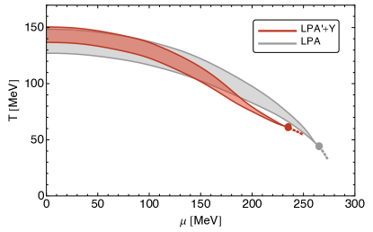
Figure 2: The phase boundaries of the chiral transition in the LPA’+Y and LPA truncations. The crossover transitions corresponds to the width of the light $\partial\bar{\sigma}_{L,k=0}/\partial T$ at 80% of its peak height. The dots mark the critical endpoints and the dotted lines the first-order transitions.

IV.2 The Phase Boundary and the Critical Endpoint

The result for the chiral phase boundary is shown in Fig. 2 wherein the red (dark) region has been obtained with the LPA^′+Y scheme. Since the transition is a crossover at small $\mu$, we show the width of the light condensate in the IR, $\partial\bar{\sigma}_{L,k=0}/\partial T$ at 80% of its peak height. The maximum at $\mu=0$ corresponds to a pseudocritical $T_{c}=144\,\text{MeV}$. The width stays almost constant until $\mu\sim 150\,\text{MeV}$ and then the transition becomes sharper for larger $\mu$. At $\mu=235\,\text{MeV}$ the width is zero and the transition is of second order. For $\mu>235\,\text{MeV}$ we find a first-order transition which is indicated by the dotted red line. Since the expansion of the effective potential is not fully converged in this region we stop the computation for $\mu>250\,\text{MeV}$. For details on the expansion we refer to App. A.

To emphasize the physical effects caused by the running Yukawa couplings and wave function renormalizations, we compare the LPA^′+Y results to the ones obtained in the LPA truncation, where these contributions are neglected. The corresponding phase boundary is given by the gray (light) band in Fig. 2. The width of the phase boundary at vanishing chemical potential is about 50% larger in LPA as compared to the LPA^′+Y truncation. Thus, the overall effect of the running Yukawa couplings and the anomalous dimensions is to sharpen the phase transition.

In order to distinguish between the various contributions of the Yukawa couplings and of the anomalous dimensions, we show in Tab. 2 the location of the critical endpoint in dependence of the three truncation schema.

truncation	$(T_{\text{CEP}},\mu_{\text{CEP}})$ [MeV]
LPA′+Y	(61, 235)
LPA+Y	(46, 255)
LPA	(44, 265)

Table 2: Location of the critical endpoint in various truncations.

In LPA it is located at $(T_{\text{CEP}},\mu_{\text{CEP}})=(44,265)$ MeV and in LPA^′+Y at $(T_{\text{CEP}},\mu_{\text{CEP}})=(61,235)$ MeV. While both the running Yukawa couplings as well as the anomalous dimensions push the CEP to smaller chemical potentials and larger temperatures, the anomalous dimensions yield the dominant contribution. The effects of the different truncations also become apparent in the quark masses which are presented in Fig. 3. Both, the Yukawa coulings and the wave function renormalizations sharpen the chiral transition. This effect is more pronounced at larger chemical potential. We conclude that the fluctuation-induced corrections to the quark and meson propagators, i.e., the wave function renormalizations, as well as quantum corrections to the quark-meson scattering processes, i.e., the running Yukawa couplings, have a substantial quantitative effect on the chiral phase boundary.

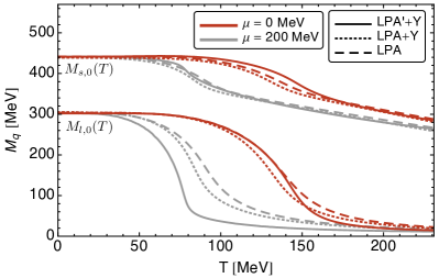
Figure 3: The light and strange quark masses in the IR as a function of temperature for the three truncations at $\mu=0$ and $\mu=200\,\text{MeV}$.

In order to deepen these observations, we investigate the temperature and chemical potential dependence of the Yukawa couplings and the wave function renormalizations in the LPA^′+Y schema. In Fig. 4 we show the temperature dependence of the meson $Z_{\phi,k=0}$ (solid lines) as well as the light quark $Z_{l,k=0}$ (dashed lines) and strange quark $Z_{s,k=0}$ (dotted lines) wave function renormalizations for $\mu=0$ (red dark lines) and $\mu=200\,\text{MeV}$ (gray light lines). They are normalized to one at vanishing temperature. As similar to two-flavor QCD studies Pawlowski and Rennecke (2014); Braun et al. (2016); Rennecke (2015a), the meson wave function renormalizations show a characteristic behavior for fields that eventually decouple from the physical spectrum. While the mesonic $Z_{\phi,k=0}$ below $T_{c}$ is almost temperature independent, it rapidly drops in the chirally symmetric phase. Since the wave function renormalizations are the prefactors in the kinetic field terms, cf. Eq. (1), this behavior signals a suppression of the mesonic fluctuations when chiral symmetry is restored. This nicely explains why the phase transition becomes steeper in this truncation: The non-trivial behavior of $Z_{\phi,k=0}$ triggers a rapid decoupling of the mesons above $T_{c}$. The symmetry restoring bosonic fluctuations that tend to wash-out the phase transition are therefore suppressed in the vicinity of the phase transition, which in turn leads to a sharper crossover transition. This tendency becomes even more pronounced at larger chemical potential as demonstrated by the solid gray line in Fig. 4: the drop-off of $Z_{\phi,k=0}$ becomes steeper with increasing $\mu$. Hence, the suppression of meson fluctuations is amplified at larger densities which also explains qualitatively why the CEP moves to smaller densities and larger temperatures.

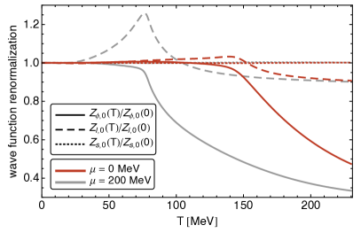
Figure 4: Meson, light and strange quark wave function renormalizations as a function of the temperature at $\mu=0$ and $\mu=200$ MeV. The strange $Z_{s,k=0}$ is almost temperature independent since it varies only about $0.4$% in the shown temperature region.

The quark wave function renormalizations show a less prominent behavior in Fig. 4. In particular, the strange quark wave function renormalization $Z_{s,k=0}$ (dashed line in the figure) barely runs and is almost insensitive to thermal and density fluctuations. The immediate consequence is that $Z_{s,k}$ could safely be ignored here. The light quark wave function renormalization $Z_{l,k=0}$ (dashed line in the figure) first grows with increasing temperature, before it decreases again above $T_{c}$. The higher the chemical potential, the higher the peak of $Z_{l,k=0}$ at $T_{c}$. Hence, light quark fluctuations are amplified through the running light quark wave function renormalizations in the vicinity of the phase transition. This effect becomes stronger with increasing $\mu$. Since fermionic fluctuations have the tendency to sharpen the chiral phase transition, the effect of the amplified quark fluctuations adds to the effect of the meson wave function renormalization as discussed above.

In Fig. 5 the temperature dependence of the light and strange quark Yukawa couplings, $\bar{h}_{l,k=0}$ (solid line) and $\bar{h}_{s,k=0}$ (dashed line) is shown at $\mu=0$ (red dark lines) and at $\mu=200\,\text{MeV}$ (gray light lines). The initial condition for $\bar{h}_{l,k}$ and $\bar{h}_{s,k}$ are tuned such that they yield the same infrared vacuum value. This ensures that the difference between the constituent masses of the light and strange quarks is solely driven by spontaneous symmetry breaking. They start to deviate in the vicinity of the critical temperature. There are two opposing contributions to the running of the Yukawa couplings. On the one hand, there is the contribution from the triangle diagrams, i.e., the terms proportional to $\bar{h}_{l,k}^{3}$ in Eq. (31) and $\bar{h}_{s,k}^{3}$ in Eq. (32). They are positive and tend to decrease the Yukawa couplings with increasing temperature. On the other hand, both flows have contributions from the anomalous dimensions. From Eq. (21) and Fig. 4 we conclude that this contribution tends to increase the Yukawa couplings with increasing temperatures. As visible in Fig. 5, the contributions from the anomalous dimensions dominate and both couplings $\bar{h}_{l,k}$ and $\bar{h}_{s,k}$ are almost constant below $T_{c}$ but increase above. The dip of $\bar{h}_{l,k=0}$ at $T_{c}$ is directly linked to the peak of $Z_{l,k=0}$ as shown in Fig. 4.

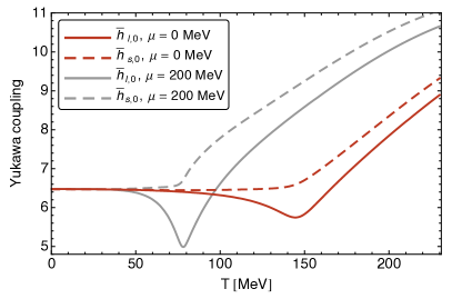
Figure 5: Light and strange quark Yukawa couplings $\bar{h}_{l,0}$ and $\bar{h}_{s,0}$ as a function of the temperature at $\mu=0$ and $\mu=200$ MeV.

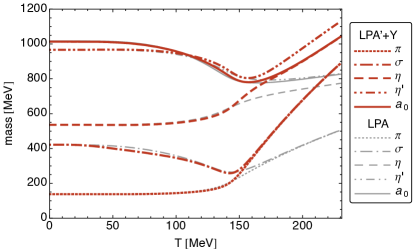
Figure 6: Meson masses as a function of the temperature at $\mu=0$ in LPA^′+Y (red lines) in comparison to the LPA result (thinner gray lines). Note, in LPA^′+Y the $a_{0}$-meson degenerates with the $\eta$-meson, while in LPA the $a_{0}$-meson and $\eta^{\prime}$-meson degenerate.

The physical effect of the meson wave function renormalizations becomes most obvious in the meson masses as exemplified in Fig. 6. To demonstrate this we compare our LPA^′+Y results (red dark lines) to the corresponding LPA result (thin gray lines). As discussed above, the quantum corrections to $Z_{\phi,k}$ drive the decoupling of the mesons in the high energy regime which is realized by rapidly rising masses for $T>T_{c}$. From Fig. 6 we conclude that the running of $Z_{\phi,k}$ is crucial to capture this physical behavior. Interestingly, in this case we also see a change of the chiral partner of the $a_{0}$-meson: While it degenerates with the $\eta^{\prime}$-meson at large temperatures in the LPA, it degenerates with the $\eta$-meson in LPA^′+Y. We will discuss this in more detail in the next section. We also observe a pronounced drop of the $\eta^{\prime}$ mass at the chiral phase transition. This is in line with experimental results on the in-medium modifications of this mass Csorgo et al. (2010); Vertesi et al. (2011). However, we emphasize that this drop can be attributed to the melting of the chiral condensates and does not indicate the restoration of $U(1)_{A}$-symmetry, as also pointed out e.g. in Heller and Mitter (2016). In a linear sigma model with a temperature dependent anomaly, a drop of the $\eta^{\prime}$ mass is not found Fejos and Hosaka (2016).

Finally, we want to discuss the systematic error of our results on the phase boundary. Firstly and most importantly, we focused on the effects of mesonic fluctuations on the phase boundary and neglected the gauge sector entirely. Thus, it is impossible to deal with the deconfinement transition in the present setup. However, it can be upgraded in this direction in a straightforward way by effectively including a non-vanishing temporal gluon background e.g. by means of a Polyakov-loop enhanced quark-meson model along the lines of Fukushima (2004); Ratti et al. (2006); Schaefer et al. (2007); Herbst et al. (2011). It has been shown in Herbst et al. (2013) that the inclusion of the Polyakov-loop potential tends to move the chiral transition line as well as the CEP to higher temperatures (see Schaefer et al. (2010); Karsch et al. (2011); Schaefer and Wagner (2012) also for similar mean-field analyses). This is reassuring since the critical temperature at vanishing chemical potential in the present work seems a little too low. Another shortcoming of the present truncation is the lack of baryonic degrees of freedom. These are certainly the dominant degrees of freedom in the high chemical potential and small temperature regime and hence they are indispensable for a realistic description of the QCD phase diagram in this regime, in particular for the liquid-gas transition to nuclear matter. However, recent DSE results indicate that baryonic degrees of freedom have only very little effect on the chiral phase boundary Eichmann et al. (2016). A direct comparison with recent DSE results on the location of the CEP Fischer et al. (2014a, b) would be involved at the present stage. For example, on the one hand gluonic effects are neglected in this FRG study while the back-coupling of mesons on the other hand is not explicitly taken into account in the DSE studies of the phase diagram Fischer and Luecker (2013). Thus, for a sensible comparison of the corresponding results an enlargement of the used truncations in both functional approaches is essential.

Lastly, another error source lies in the experimental identification of the proper chiral $\sigma$-meson. The precise location of the CEP is rather sensitive to the mass value of the $\sigma$-meson Schaefer and Wagner (2009), which we identified with the $f_{0}(500)$ resonance, whose mass is between $400-550\,\text{MeV}$ Olive et al. (2014). We have chosen $M_{\sigma}=421$ MeV and for larger values the CEP moves to larger chemical potential and smaller temperature. Furthermore, it is still controversial whether the $\sigma$-meson should be identified with the $f_{0}(500)$ or with the $f_{0}(1370)$ resonance. It was argued e.g. in Parganlija et al. (2010) that the latter option might be favored and the $f_{0}(500)$ resonance could be identified with a tetraquark state Jaffe (1977). However, within the FRG treatment it is not possible to find a physically sensible set of initial conditions that allow for an identification of the $\sigma$-meson with the $f_{0}(1370)$, see also Eser et al. (2015). If one would increase $M_{\sigma}$ by increasing the initial value of $\bar{\lambda}_{20,k=\Lambda}$ the UV masses of the other mesons would decrease again. But as argued in Sec. IV.1, these masses have to be larger than the UV cutoff to ensure a suppression of the meson fluctuation in the chirally symmetric regime. We find that this requirement excludes values larger than $M_{\sigma}\gtrsim 600\,\text{MeV}$. Hence, identifying the $\sigma$-meson with the $f_{0}(1370)$ within our present setup is at odds with initial conditions consistent with QCD.

IV.3 Pseudoscalar Mixing and the Axial Anomaly

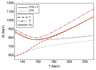
Figure 7: The masses of $\eta$-, $\eta^{\prime}$- and $a_{0}$-meson at large temperatures. While the $a_{0}$-meson (solid lines) degenerates with the $\eta^{\prime}$-meson in LPA (thin dotted-dashed gray line), it degenerates with the $\eta$-meson in LPA^′+Y (dashed red dark line).

As already mentioned (cf. Fig. 6) the chiral partner of the $a_{0}$-meson is the $\eta$-meson rather than the $\eta^{\prime}$-meson in LPA^′+Y, which is displayed in more detail in Fig. 7. This finding is in contradistinction to results found in a linear sigma model Lenaghan et al. (2000) and in quark-meson models Schaefer and Wagner (2009); Tiwari (2013) in mean-field approximation, as well as an FRG investigation with the quark-meson model in LPA Mitter and Schaefer (2014). The reason is that in particular the fluctuation-induced corrections to the meson propagators lead to the opposite pseudoscalar mixing at large temperatures compared to computations where these corrections are ignored. The pseudoscalar mixing angle $\varphi_{p}$ describes the composition of the physical $\eta$- and $\eta^{\prime}$-states in terms of the purely light $\eta_{L}$ and strange $\eta_{S}$ states, i.e., it describes the light and strange quark content of the physical states, see Eq. (13). The mixing angles as a function of the temperature for vanishing density are shown in Fig. 8 where the scalar (dashed lines) and the pseudoscalar (solid lines) mixing angles obtained in LPA^′+Y (red dark lines) are compared to the LPA results (gray light lines). The scalar mixing angles $\varphi_{s}$ differ only mildly in both truncations in contrast to the pseudoscalar mixing angle $\varphi_{p}$ for temperatures above $T_{c}$. For a related DSE analysis of the pseudoscalar mixing angle, see e.g. Horvatic et al. (2007).

If we ignore the running wave function renormalizations and the Yukawa couplings, $\varphi_{p}$ grows for $T>T_{c}$ towards the ideal mixing $\varphi_{p}\rightarrow 90^{\circ}$ (solid gray light line in Fig. 8). This implies that the $\eta$-meson becomes a purely strange state and the $\eta^{\prime}$-meson a purely light state when chiral symmetry is restored. Hence, the $\eta^{\prime}$ degenerates with the light $a_{0}$-state at large temperatures in LPA. Similar for the scalar sector: since $\varphi_{s}$ approaches ideal mixing in both truncations, the $\sigma$-meson is a purely light and the $f_{0}$-meson a purely strange state. Hence, the chiral partner of the $f_{0}$ is the $\eta$-meson in LPA. However, since the strange condensate melts only very slowly (cf. Fig. 3) we do not observe this degeneration in the considered temperature range. This is in line with results in the literature, e.g. Lenaghan et al. (2000); Schaefer and Wagner (2009) when quantum corrections to the classical dispersion relation of the mesons, directly related to $Z_{\phi,k}$, are neglected.

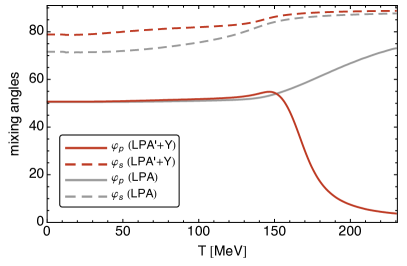
Figure 8: The scalar and pseudoscalar mixing angles $\varphi_{p,s}$ as a function of temperature at vanishing density in LPA^′+Y (red lines) in comparison to the LPA results (gray lines). The $\eta$-meson becomes a purely light state at large temperatures and the $\eta^{\prime}$-meson a purely strange state.

If we include these corrections by employing the LPA^′+Y truncation, we find that $\varphi_{p}$ first slightly grows with temperature until $T_{c}$ similar to the LPA result. $\varphi_{p}$ stays close to 54^∘ for $T\lesssim T_{c}$ meaning that the $\eta$ is an almo st ideal flavor octet state and $\eta^{\prime}$ an almost ideal flavor singlet state. Above $T_{c}$ the pseudoscalar mixing angle rapidly drops and finally approaches "anti-ideal" mixing $\varphi_{p}\rightarrow 0^{\circ}$ at large temperatures (red dark solid line in Fig. 8). Hence, $\eta$ becomes a purely light state with $a_{0}$ as its chiral partner and $\eta^{\prime}$ becomes purely strange with $f_{0}$ as chiral partner. Again, we do not observe the degeneration of $\eta^{\prime}$ with $f_{0}$ within the considered temperature range due to the slow melting of the strange condensate (cf. Fig. 3). In Tab. 3 we summarized our findings.

mean-field/LPA/LPA+Y	LPA′ + Y
$(\eta,f_{0})$	$(\eta,a_{0})$
$(\eta^{\prime}\!\!,a_{0})$	$(\eta^{\prime}\!\!,f_{0})$

Table 3: Chiral partners for different approximations.

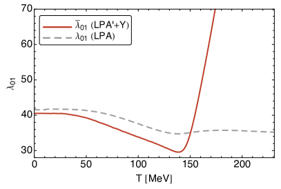
Figure 9: Temperature-dependence of the quartic meson coupling, which enters the pseudoscalar mixing angle, at vanishing density in LPA^′+Y (solid red line) and in LPA (dashed gray line).

We can further elucidate this phenomenon by examining the analytical structure of the mixing angle. For convenience we restrict our discussion to the 08-basis and call the pseudoscalar mixing angle $\Theta_{p}$ that maps from the 08-basis to the physical one, see App. C for details. Furthermore, we concentrate the discussion without any limitations to vanishing density because the mixing angle behaves similarly at finite $\mu$. According to (14) we have the relation $\varphi_{p}=\Theta_{p}+\arctan\sqrt{2}$ which yields with Eq. (70) and the expressions in App. D for $k=0$:

$$\tan 2\Theta_{p}=2\sqrt{2}\,\frac{\big{(}\sqrt{2}\bar{\sigma}_{S}-\bar{\sigma}_{L}\big{)}\,\bar{c}-\big{(}2\bar{\sigma}_{S}^{2}-\bar{\sigma}_{L}^{2}\big{)}\bar{\lambda}_{01}}{\big{(}\sqrt{2}\bar{\sigma}_{S}+8\bar{\sigma}_{L}\big{)}\,\bar{c}-\big{(}2\bar{\sigma}_{S}^{2}-\bar{\sigma}_{L}^{2}\big{)}\bar{\lambda}_{01}}\,.$$ (42)

The quartic meson coupling in the infrared related to $\bar{\tilde{\rho}}_{2}$ is given by $\bar{\lambda}_{01}={\partial\bar{U}_{k=0}}/{\partial\bar{\tilde{\rho}}_{2}}\Big{|}_{\Phi_{0}}$.

Hence, $\Theta_{p}$ is solely driven by the condensates and the running of $\bar{\lambda}_{01}$ because the KMT coupling $\bar{c}$ is a constant as explained in Sec. III.2. The temperature dependence of $\bar{\lambda}_{01}$ in LPA^′+Y and LPA are shown in Fig. 9. At vanishing temperature $\Theta_{p}$ is small and negative since the light and strange condensates are almost identical, $\bar{c}$ is constant and $\bar{\lambda}_{01,k}\approx 40$ in both LPA and LPA^′+Y truncations cf. Fig. 9 and Tab. 1. This means that the $\eta^{\prime}$-state is mostly a $SU(3)$ singlet state at $T\lesssim T_{c}$. With rising temperature, $\bar{\sigma}_{L}$ melts much faster than $\bar{\sigma}_{S}$ and $\bar{\lambda}_{01}$ drops towards $T_{c}$ which yields in an overall increase of the mixing angle. Thus, for $T\lesssim T_{c}$ the mixing angle shows a similar behavior in both truncations. But for $T>T_{c}$ the quartic coupling stays almost constant in LPA while it grows rapidly in LPA^′+Y. The behavior of the mixing angle in LPA is therefore dominated by the melting of the condensates. In this case, the mixing angle tends to an ideal mixing $\varphi_{p}\rightarrow 90^{\circ}$ since the light condensate becomes negligible over the strange condensate and hence $\tan 2\Theta_{p}\rightarrow 2\sqrt{2}$ at large temperature.

In LPA^′+Y, however, the quartic coupling $\bar{\lambda}_{01}$ grows much faster than the difference of the strange and light condensate at $T>T_{c}$. As a consequence, Eq. (42) is dominated by $\bar{\lambda}_{01}$ and the mixing angle decreases with increasing temperature in this regime. The denominator of Eq. (42) decreases until it vanishes around $T\approx 194\,\text{MeV}$ and $\tan 2\Theta_{p}\rightarrow 2\sqrt{2}$ at larger temperatures because, again, the light condensate becomes negligible over the strange condensate. Note, however, that by continuity the branch of the complex tangent function has changed and thus the equation $\tan 2\Theta_{p}=2\sqrt{2}$ implies an anti-ideal mixing $\varphi_{p}=0^{\circ}$. The rapid rise of $\bar{\lambda}_{01}$ in Fig. 9 is directly linked to the rapid drop of $Z_{\phi,k=0}$ in Fig. 4: Reparametrization invariance implies the relation $\bar{\lambda}_{01}=\lambda_{01}/Z_{\phi,k=0}^{2}$. Since these improvements are neglected in standard mean-field studies of linear sigma and quark-meson models and in LPA with the FRG, such a behavior of the mixing angle could not be observed in these cases. In particular, in studies where quantum fluctuations are taken into account, it is crucial to capture the dynamical change of the relevant fluctuating degrees of freedom for a proper description of the phase transitions.

We have demonstrated that overestimating meson fluctuations in the vicinity of the chiral phase transition by not accounting for their proper decoupling from the physical spectrum above $T_{c}$ leads to a wrong assignment of the chiral partners of the ($\eta$, $\eta^{\prime}$) complex. The underlying mechanism is particularly lucid here. The behavior of $Z_{\phi,k=0}$ should be generic for QCD in the high-energy regime such that a similar behavior of the mixing angle is expected in full QCD.

Interestingly, the same qualitative behavior of the pseudoscalar mixing angle has been observed in a Nambu–Jona-Lasinio (NJL) model study including the axial anomaly in mean-field approximation Costa et al. (2005). Moreover, similar findings were obtained for a Polyakov-loop augmented quark-meson model with vector mesons in an extended mean-field approximation where fermionic vacuum fluctuations are additionally considered Kovacs et al. (2016). These results are in general in line with our discussion above. However, we note that the main difference between Kovacs et al. (2016) and Tiwari (2013) is the incorporation of vector mesons on the mean-field level in the former case. Yet, while $\varphi_{p}$ in Kovacs et al. (2016) behaves qualitatively similar as in our LPA^′+Y truncation, it behaves as in LPA in Tiwari (2013). This might be related to the different input parameters in the presence of vector mesons. In terms of fluctuations, however, recent studies beyond mean-field clearly indicate the irrelevance of the vector meson dynamics in Euclidean spacetime Rennecke (2015a); Eser et al. (2015); Jung et al. (2017). Thus, even though different parameterizations of effective models can influence the value of the mixing angle, the dynamical effect identified in this work is expected to be relevant in any case.

Finally, the observation of this phenomenon is directly related to the presence of the axial anomaly. In absence of the anomaly, i.e. when $\bar{c}=0$, the pseudoscalar mixing angle stays constant since $\tan 2\Theta_{p}=2\sqrt{2}$ (cf. Eq. (42)). Thus, the non-trivial behavior of $\varphi_{p}$ as observed in Fig. 8 can only appear when $\bar{c}\neq 0$ i.e. in the presence of the axial anomaly. We remark that this observation may be an artifact of our model. A thorough study of the axial anomaly is beyond the scope of the present work.

V Conclusions and Outlook

We have investigated the influence of quantum and thermal fluctuations on the chiral phase structure in the low-energy sector of QCD. Motivated by the importance of mesonic degrees of freedom in QCD at low energies, we employed an effective $N_{f}=2+1$ quark-meson model and incorporated quantum, thermal and density fluctuations by means of the functional renormalization group. The main focus was the investigation of the impact of quark and meson fluctuation-induced corrections to the classical quark and meson dispersion relations as well as to quark-meson interactions. To this end, we allowed for running light quark, strange quark and meson wave function renormalizations $Z_{q/\phi,k}$ as well as running light and strange quark Yukawa couplings $h_{q,k}$ and computed the resulting full effective potential. Our two main findings were:

The considered fluctuations have an important and substantial impact on the chiral phase boundary. The crossover transition is significantly sharper as compared to computations that ignore the running of the wave function renormalizations and the Yukawa couplings (LPA truncation), see e.g. Schaefer and Wambach (2007, 2005) for similar two-flavor FRG investigations. Furthermore, the location of the critical endpoint is pushed towards smaller density and larger temperature. The overall quantitative effect on the chiral phase boundary of these fluctuation-effects is substantial.

The pseudoscalar mixing angle, which determines the quark content of the pseudoscalar mesons, turned out to depend crucially on the elaborated interplay between quark and meson fluctuations. This is intimately related to chiral symmetry restoration and the presence of the axial anomaly. As a result, while the $\eta$- and $\eta^{\prime}$-mesons are almost ideal flavor octet and singlet states below $T_{c}$, the mixing angle approaches an anti-ideal flavor mixing at temperatures above $T_{c}$ if all fluctuation corrections are taken into account (LPA^′+Y truncation). The $\eta$-meson becomes a purely light quark composite and $\eta^{\prime}$ purely strange. In absence of the axial anomaly, the $\eta^{\prime}$ degenerates with the pions above $T_{c}$ and therefore becomes a light quark state. As a consequence, a rearrangement of the chiral meson partner $(a_{0},\eta)$ and $(f_{0},\eta^{\prime})$ occurs in the presence of the axial anomaly. However, we consolidated this observation by clarifying its direct connection to the running of the meson wave function renormalization $Z_{\phi,k}$. We thus expect that our findings are also qualitatively incorporated in full QCD and describe more realistically the relevant physical superposition of gluon and hadron effects including their mutual back-reaction in particular in the transition region.

Of course there is still space for further improvements: the neglected gluon fluctuations can at least effectively included in this framework by a non-vanishing temporal gluon background yielding Polyakov-loop augmented quark-meson model truncations Schaefer et al. (2007, 2010); Karsch et al. (2011). This enables additionally the analysis of deconfinement issues in the same setup as discussed in Sec. IV.2. Another important aspect is the unknown significance of baryon degrees of freedom at finite densities and their influence on the location of a possible critical endpoint. A first exploratory study in a DSE framework wherein quark and gluon fluctuations are taken into account indicates that baryons seems to have only little impact on the location of the CEP in the phase diagram Eichmann et al. (2016).

Aiming at a more accurate description of QCD along the lines of e.g. Herbst et al. (2011); Mitter et al. (2015); Braun et al. (2016) as well as phenomenological applications such as baryon and strangeness fluctuations are obvious directions for future work.

Acknowledgments - We thank Mario Mitter, Jan M. Pawlowski and Simon Resch for discussions and collaboration on related projects. This work has been supported by the FWF grant P24780-N27, the Helmholtz International Center for FAIR within the LOEWE program of the State of Hesse and by the DFG Collaborative Research Centre "SFB 1225 (ISOQUANT)".

Appendix A Two-Dimensional Fixed Background Taylor Expansion

There are various ways to solve the flow equation for the field dependent effective potential $U_{k}(\rho_{1},\tilde{\rho}_{2})$. Most common choices are either to discretize the potential in field space or perform a Taylor expansion. While the former provides very accurate information about the global potential structure, the latter only gives accurate local information about the potential and its derivatives in the vicinity of the expansion point. Even though the full global information is only hardly accessible within a Taylor expansion, it is numerically less extensive. While an expansion about the running minimum of the effective potential seems to be the most natural choice, its convergence properties are rather poor as has been demonstrated in Pawlowski and Rennecke (2014). A static expansion about a scale-independent point which coincides with the IR-minimum of the effective potential is numerically more stable and converges rapidly.

Here, we generalize this static background Taylor expansion to two dimensions. We expand the effective potential $\tilde{U}_{k}(\rho_{1},\tilde{\rho}_{2})$ about two scale-independent expansion points $\kappa_{1}$, $\kappa_{2}$ to a given order $N$

$$U_{k}(\rho_{1},\tilde{\rho}_{2})=\sum_{i,j=0}^{N}\frac{\lambda_{ij,k}}{i!j!}(\rho_{1}-\kappa_{1})^{i}(\tilde{\rho}_{2}-\kappa_{2})^{j}$$ (43)

with $\lambda_{00,k}=0$. There are various way to define this expansion: while an expansion directly in powers of the chiral invariants seems to be the easiest choice, an expansion in powers of the fields is more natural. We also found the latter to be numerically more stable. In the present case $N$ fixes the order of the fields, i.e., $i,j\in\{0,1,\dots,N+1\}$ with $0<i\!+\!2j\leq N\!+\!1$. This corresponds to an expansion up to $\phi^{2(N+1)}$ .

The RG-invariant expansion points $\bar{\kappa}_{1,k}=Z_{\phi,k}\kappa_{1}$ and $\bar{\kappa}_{2,k}=Z_{\phi,k}^{2}\kappa_{2}$ then lead to the following running of these points:

$$\partial_{t}\bar{\kappa}_{1,k}=-\eta_{\phi,k}\bar{\kappa}_{1,k}\,,\qquad\partial_{t}\bar{\kappa}_{2,k}=-2\eta_{\phi,k}\bar{\kappa}_{2,k}\,.$$ (44)

The initial values for these flow equations are chosen such that their IR values coincide with the minimum of the effective potential in light and strange dimension more precisely with the chiral invariants at the physical point

$$\begin{split}\bar{\rho}_{1,k}&=\frac{1}{2}\left(\bar{\sigma}_{L,k}^{2}+\bar{\sigma}_{S,k}^{2}\right)\,,\\ \tilde{\bar{\rho}}_{2,k}&=\frac{1}{24}\left(\bar{\sigma}_{L,k}^{2}-2\bar{\sigma}_{S,k}^{2}\right)^{2}\,,\end{split}$$ (45)

where we demand

$$\bar{\kappa}_{1,0}=\bar{\rho}_{1,0}\,,\quad\text{and}\quad\bar{\kappa}_{2,0}=\tilde{\bar{\rho}}_{2,0}\,.$$ (46)

To extract the condensates $\bar{\sigma}_{L,k}$ and $\bar{\sigma}_{S,k}$ one has to invert Eq. (45). Even though this is not unique in general, at the physical point we always have $\bar{\sigma}_{L,k}\leq\sqrt{2}\bar{\sigma}_{S,k}$ with the unique solution

$$\begin{split}\bar{\sigma}_{L,k}&=\sqrt{\frac{2}{3}\left(2\bar{\rho}_{1,k}-\sqrt{6\tilde{\bar{\rho}}_{2,k}}\right)}\,,\\ \bar{\sigma}_{S,k}&=\sqrt{\frac{2}{3}\left(\bar{\rho}_{1,k}+\sqrt{6\tilde{\bar{\rho}}_{2,k}}\right)}\,.\end{split}$$ (47)

In practice, we fine-tune the initial conditions for the expansion points $\bar{\kappa}_{1,k=\Lambda}$ and $\bar{\kappa}_{2,k=\Lambda}$ such that

$$\begin{split}\bar{\sigma}_{L,k=0}\,<\,\sqrt{\frac{2}{3}\left(2\bar{\kappa}_{1,k=0}-\sqrt{6\kappa_{2,k=0}}\right)}\,&\leq\,(1+\epsilon)\,\bar{\sigma}_{L,k=0}\,,\\ \bar{\sigma}_{S,k=0}\,<\,\sqrt{\frac{2}{3}\left(\bar{\kappa}_{1,k=0}+\sqrt{6\kappa_{2,k=0}}\right)}\,&\leq\,(1+\epsilon)\,\bar{\sigma}_{S,k=0}\,,\end{split}$$ (48)

where we typically choose $\epsilon$ of the order of $5\cdot 10^{-4}$. For the numerical stability of the expansion it is crucial that the expansion points do not lie in the convex region of the effective potential for $k\rightarrow 0$. However, being close to the physical minimum is indispensable if the truncation of the effective action contains field-independent parameters since the parameters obtain a physical meaning only when they are defined at the physical point in the IR. Here, this is the case for the wave function renormalizations and the Yukawa couplings. If one would also expand these terms, one only needs to choose the expansion points such that the physical point lies within the radius of convergence of the expansion, which would allow for much larger values for $\epsilon$. For more details see Pawlowski and Rennecke (2014).

The flow equations of the expansion coefficients in Eq. (43) are:

$$\partial_{t}\bar{\lambda}_{nm,k}=(n+2m)\eta_{\phi,k}\bar{\lambda}_{nm,k}+\frac{\partial^{n+m}\partial_{t}U_{k}(\rho_{1},\tilde{\rho}_{2})}{\partial\rho_{1}^{n}\partial\tilde{\rho}_{2}^{m}}\bigg{|}_{\kappa_{1},\kappa_{2}}\,,$$ (49)

where $\partial_{t}U_{k}(\rho_{1},\tilde{\rho}_{2})$ is given by Eq. (26). We have used $N=4$ (corresponding to a $\phi^{10}$-expansion) throughout this work. We found that our results are independent of $N$ for $N\geq 3$ and $\mu\lesssim 250\,\text{MeV}$. At larger $\mu$, the distance between the local minima of the effective potential in the region of the first-order phase transition appears to be larger than the radius of convergence of the expansion at $N=4$. Hence, we do not resolve the phase boundary at larger chemical potential.

We want to end with a discussion of the field dependence of the flow equation. In general, it can be a complicated non-linear function of various invariants, including potential non-analytical terms. This can be inferred, e.g., from Eq. (47) and was also discussed in Patkos (2012). There, it was shown that higher powers of an expansion of the effective potential in terms of the invariants $\rho_{1}$ and $\tilde{\rho}_{2}$ indeed contain fractional powers of the invariants. It was argued that they arise due to the omission of the third invariant. However, the fast convergence of our expansion suggests that we do not suffer from any non-analyticities within the range of parameters we consider here. Furthermore, we are able to accurately reproduce the results of Mitter and Schaefer (2014), wherein the flow of the $U(3)\!\times\!U(3)$-symmetric part of the effective potential was solved on a two-dimensional grid of the two invariants $\rho_{1}$ and $\tilde{\rho}_{2}$ in the LPA truncation. Aside from the physical requirement that the effective potential is a function of the chiral invariants, no assumptions are made about the functional form of the potential. This method captures the full field dependence of the effective potential, including potential non-analyticities. Owing to the fast convergence of our expansion and the reproduction of the results in Mitter and Schaefer (2014) we are confident that we accurately solve the flow of the effective potential at the physical point within our truncation.

Furthermore, we again want to emphasize that the assumption that the anomaly coefficient $\bar{c}$ is not running is part of our truncation. In principle, one could extract a flow of this coupling from the effective potential by considering an appropriate three-point function. This is beyond the scope of the present work. An elegant way to disentangle and extract the flow of the anomaly coefficient as well as to close the set of flow equations in the LPA truncation of a linear sigma model is presented in Fejos and Hosaka (2016).

Appendix B Threshold Functions

In this appendix the regulators and threshold functions of the flow equations are specified. We restrict ourselves to $d=4$ dimensions. For the light and strange quarks as well as the mesons the following three-dimensional regulators are used so that only the spatial momenta are regulated

$$\begin{split}R_{k}^{q}(\vec{p})&=Z_{q,k}\,\vec{\gamma}\vec{p}\,r_{F}\left(\vec{p}^{2}/k^{2}\right)\,\\ R_{k}^{\phi}(\vec{p}^{2})&=Z_{\phi,k}\,\vec{p}^{2}\,r_{B}\left(\vec{p}^{2}/k^{2}\right)\end{split}$$ (50)

with the optimized fermionic $r_{F}(x)$ and bosonic $r_{B}(x)$ regulator shape functions Litim and Pawlowski (2006); Litim (2001, 2000) ($x=\vec{p}^{2}/k^{2}$)

$$\begin{split}r_{F}(x)&=\left(\frac{1}{\sqrt{x}}-1\right)\Theta(1-x)\,,\\ r_{B}(x)&=\left(\frac{1}{x}-1\right)\Theta(1-x)\,.\end{split}$$ (51)

As mentioned in Sec. III.1, the regulator ensures both UV and IR regularity of our theory. Finite temperature is implemented via the imaginary time formalism. Hence, the loop frequency integration is a sum over Matsubara frequencies $\omega_{n}=2\pi nT$ and $\nu_{n}=2\pi(n+1/2)T$ for bosons and fermions respectively. At large temperatures the meson contributions reduce to the three-dimensional case due to dimensional reduction. Since the quark propagators vanish for $p_{0}\rightarrow\infty$, the quark contributions are also UV regular.

With these regulators, the scalar parts without the tensor structure of the quark and meson propagators read

$$\begin{split}\bar{G}_{q,k}(\nu_{n},\vec{p})&=\frac{\Theta(k^{2}-\vec{p}^{2})}{Z_{q,k}\big{(}(\nu_{n}+i\mu)^{2}+k^{2}\big{)}+m_{q,k}^{2}}\\ &\quad+\frac{\Theta(\vec{p}^{2}-k^{2})}{Z_{q,k}\big{(}(\nu_{n}+i\mu)^{2}+\vec{p}^{2}\big{)}+m_{q,k}^{2}}\,,\\ \bar{G}_{\phi,k}(\omega_{n},\vec{p})&=\frac{\Theta(k^{2}-\vec{p}^{2})}{Z_{\phi,k}\big{(}\omega_{n}^{2}+k^{2}\big{)}+m_{\phi,k}^{2}}\\ &\quad+\frac{\Theta(\vec{p}^{2}-k^{2})}{Z_{\phi,k}\big{(}\omega_{n}^{2}+\vec{p}^{2}\big{)}+m_{\phi,k}^{2}}\,.\end{split}$$ (52)

In the spirit of the low-momentum expansion all flow equations are evaluated at vanishing spatial external momenta, cf. e.g. Eq. (30). As a consequence, only the parts of the propagators proportional to $\Theta(k^{2}-\vec{p}^{2})$ will contribute to the final flow equations. Hence, in the following we will use the dimensionless RG-invariant propagators

$$\begin{split}\tilde{G}_{q,k}(p_{0})&=\frac{1}{(p_{0}+i\mu)^{2}/k^{2}+1+\bar{m}_{q,k}^{2}}\,,\\ \tilde{G}_{\phi,k}(p_{0})&=\frac{1}{p_{0}^{2}/k^{2}+1+\bar{m}_{\phi,k}^{2}}\,,\end{split}$$ (53)

which directly enter the loop frequency summations.

The functions $l_{0}^{(B/F)}$ in Eq. (26) are related to the bosonic/fermionic loops and are defined as

$$l_{0}^{(B)}(\bar{m}_{\phi,k}^{2},\eta_{\phi,k})$$ (54)

$$=\frac{T}{2k}\sum_{n\in\mathbb{Z}}\int\!dxx^{\frac{3}{2}}\left(\partial_{t}r_{B}(x)-\eta_{\phi,k}r_{B}(x)\right)\tilde{G}_{\phi,k}(\omega_{n})$$

$$=\frac{2}{3}\frac{k}{E_{\phi,k}}\left(1-\frac{\eta_{\phi,k}}{5}\right)\left(\frac{1}{2}+n_{B}(E_{\phi,k})\right)\,,$$

for mesons and

$$l_{0}^{(F)}(\bar{m}_{q,k}^{2},\eta_{q,k})$$ (55)

$$=\frac{T}{k}\sum_{n\in\mathbb{Z}}\int\!\!\!dxx^{\frac{3}{2}}\left(\partial_{t}r_{F}(x)-\eta_{q,k}r_{F}(x)\right)(1+r_{F}(x))\tilde{G}_{q,k}(\nu_{n})$$

$$=\frac{1}{3}\frac{k}{E_{q,k}}\left(1-\frac{\eta_{q,k}}{4}\right)\Big{[}1-n_{F}(E_{q,k}-\mu)-n_{F}(E_{q,k}+\mu)\Big{]}\,,$$

for quarks with the usual Bose and Fermi distributions

$$\begin{split}n_{B}(E)=\frac{1}{e^{E/T}-1}\,,\quad n_{F}(E)=\frac{1}{e^{E/T}+1}\,,\end{split}$$ (56)

and the scale dependent quasiparticle energies

$$E_{\Phi,k}=k\sqrt{1+\bar{m}_{\Phi,k}^{2}}\,\qquad\text{with}\qquad\bar{m}_{\Phi,k}=M_{\Phi,k}/k\,.$$ (57)

The threshold functions $L_{(1,1)}$ that appear in the flows of the Yukawa couplings, (31) and (32), are related to the triangle diagrams as shown in Fig. 1(a). They are defined by

$$\begin{split}&L_{(1,1)}\left(\bar{m}_{q,k}^{2},\bar{m}_{\phi,k}^{2},\eta_{q,k},\eta_{\phi,k};p_{0}\right)\\ &=\frac{T}{2k}\sum_{n\in\mathbb{Z}}\int\!dxx^{\frac{3}{2}}\bigg{[}\left(\partial_{t}r_{B}(x)-\eta_{\phi,k}r_{B}(x)\right)\\ &\quad\times\tilde{G}_{q,k}(\nu_{n}+p_{0})\tilde{G}_{\phi,k}^{2}(\omega_{n})+2\big{(}1+r_{F}(x)\big{)}\\ &\quad\times\left(\partial_{t}r_{F}(x)-\eta_{q,k}r_{F}(x)\right)\tilde{G}_{q,k}^{2}(\nu_{n}+p_{0})\tilde{G}_{\phi,k}(\omega_{n})\bigg{]}\,.\end{split}$$ (58)

As already mentioned we evaluate all flows at vanishing external spatial momenta and only the external frequency $p_{0}$ is retained. Owing to the optimized 3d regulators, the spatial integration can be performed analytically

$$\begin{split}&L_{(1,1)}\left(\bar{m}_{q,k}^{2},\bar{m}_{\phi,k}^{2},\eta_{q,k},\eta_{\phi,k};p_{0}\right)\\ &=\frac{2}{3}\left[\!\left(1-\frac{\eta_{\phi,k}}{5}\right)\!\textit{FB}_{(1,2)}^{(q,\phi)}+\!\left(1-\frac{\eta_{q,k}}{4}\right)\!\textit{FB}_{(2,1)}^{(q,\phi)}\right]\,,\end{split}$$ (59)

where we have suppressed the arguments of $\textit{FB}_{(1,2)}^{(q,\phi)}=\textit{FB}_{(1,2)}(\bar{m}_{q,k}^{2},\bar{m}_{\phi,k}^{2};p_{0})$. The remaining Matsubara summation can also be performed analytically with the result

$$\textit{FB}_{(1,1)}(\bar{m}_{q,k}^{2},\bar{m}_{\phi,k}^{2};p_{0})$$ (60)

$$=\frac{T}{k}\operatorname{Re}\left[\sum_{n\in\mathbb{Z}}\tilde{G}_{q,k}(\nu_{n}+p_{0})\tilde{G}_{\phi,k}(\omega_{n})\right]$$

$$=\text{Re}\,\Bigg{[}\frac{k}{2E_{\phi,k}}n_{B}(E_{\phi,k})\frac{k^{2}}{E_{q,k}^{2}-\big{(}E_{\phi,k}-ip_{0}+\mu\big{)}^{2}}$$

$$\quad+\frac{k}{2E_{\phi,k}}\big{(}n_{B}(E_{\phi,k})+1\big{)}\frac{k^{2}}{E_{q,k}^{2}-\big{(}E_{\phi,k}+ip_{0}-\mu\big{)}^{2}}$$

$$\quad-\frac{k}{2E_{q,k}}n_{F}(E_{q,k}-\mu)\frac{k^{2}}{E_{\phi,k}^{2}-\big{(}E_{q,k}+ip_{0}-\mu\big{)}^{2}}$$

$$\quad-\frac{k}{2E_{q,k}}\big{(}n_{F}(E_{q,k}+\mu)-1\big{)}\frac{k^{2}}{E_{\phi,k}^{2}-\big{(}E_{q,k}-ip_{0}+\mu\big{)}^{2}}\Bigg{]}\,.$$

The functions $\textit{FB}_{(n,m)}^{(q,\phi)}$ correspond to the Matsubara sum of $n$ quarks propagators and $m$ meson propagators and can easily be obtained from the function $\textit{FB}_{(1,1)}^{(q,\phi)}$ via derivatives

$$\textit{FB}_{(n,m)}^{(q,\phi)}=\frac{(-1)^{n+m-2}}{(n-1)!(m-1)!}\frac{\partial^{n+m-2}\textit{FB}_{(1,1)}^{(q,\phi)}}{\partial(\bar{m}_{q,k}^{2})^{n-1}\partial(\bar{m}_{\phi,k}^{2})^{m-1}}\,,$$ (61)

with $n,m\geq 1$. Note that these functions also enter the light and strange quark anomalous dimensions Eqs. (36) and (III.4).

Due to the complex frequency arguments, the real part in Eq. (60) has to be taken in order to ensure real-valued Yukawa couplings and quark anomalous dimensions which also avoids an unphysical complex-valued effective potential. For fermionic frequencies the choice $p_{0,\text{ext}}=0$ is excluded. However, as discussed in the main text, we choose $p_{0,\text{ext}}=\pi T-i\mu$, see Eq. (30). The inclusion of the fully frequency-dependent quark anomalous dimension into the effective potential results in a manifestly real effective potential. But this is beyond the scope of the present work and we refer to Fu et al. (2016) for further details.

The functions $\textit{BB}_{(n,m)}^{(\phi_{1},\phi_{2})}$ in the meson anomalous dimension (40) encodes the Matsubara summation of loops with two different meson propagators and are defined as:

$$\begin{split}&\textit{BB}_{(1,1)}(\bar{m}_{\phi_{1},k}^{2},\bar{m}_{\phi_{2},k}^{2})\,=\,\frac{T}{k}\sum_{n\in\mathbb{Z}}\tilde{G}_{\phi_{1}}(\omega_{n})\tilde{G}_{\phi_{2}}(\omega_{n})\\ &=\frac{k^{3}}{(E_{\phi_{2},k}^{2}-E_{\phi_{1},k}^{2})\,E_{\phi_{1},k}}\left(n_{B}(E_{\phi_{1},k})+\frac{1}{2}\right)\\ &\quad+\frac{k^{3}}{(E_{\phi_{1},k}^{2}-E_{\phi_{2},k}^{2})\,E_{\phi_{2},k}}\left(n_{B}(E_{\phi_{2},k})+\frac{1}{2}\right)\,.\end{split}$$ (62)

This definition is only valid for $\bar{m}_{\phi_{1},k}\neq\bar{m}_{\phi_{2},k}$. In the case of a mass degeneracy $\bar{m}_{\phi_{1},k}=\bar{m}_{\phi_{2},k}\equiv\bar{m}_{\phi,k}$ one has to use

$$\begin{split}&\textit{BB}_{(1,1)}(\bar{m}_{\phi,k}^{2},\bar{m}_{\phi,k}^{2})=-\frac{\partial}{\partial\bar{m}_{\phi,k}^{2}}\left[\frac{k}{E_{\phi,k}}\left(n_{B}(E_{\phi_{2},k})+\frac{1}{2}\right)\right]\,.\end{split}$$ (63)

Accordingly, for $n$ propagators of $\phi_{1}$ and $m$ propagators of $\phi_{2}$ we find

$$\textit{BB}_{(n,m)}^{(\phi_{1},\phi_{2})}=\frac{(-1)^{n+m-2}}{(n-1)!(m-1)!}\frac{\partial^{n+m-2}\textit{BB}_{(1,1)}^{(\phi_{1},\phi_{2})}}{\partial(\bar{m}_{\phi_{1},k}^{2})^{n-1}\partial(\bar{m}_{\phi_{2},k}^{2})^{m-1}}\,.$$ (64)

The Matsubara summation of loops with several identical fermions also enters in Eq. (40) and is encoded in:

$$\begin{split}&\textit{F}_{(1)}(\bar{m}_{q,k}^{2})\,=\,\frac{T}{k}\sum_{n\in\mathbb{Z}}\tilde{G}_{q}(\nu_{n})\\ &=\frac{k}{2E_{q,k}}\Big{[}1-n_{F}(E_{q,k}-\mu)-n_{F}(E_{q,k}+\mu)\Big{]}\,,\end{split}$$ (65)

and

$$\textit{F}_{(n)}^{\,(q)} =\frac{(-1)^{n-1}}{(n-1)!}\frac{\partial^{n-1}\textit{F}_{(1)}^{\,(q)}}{\partial(\bar{m}_{q,k}^{2})^{n-1}}\,.$$ (66)

Note that this function is implicitly contained in the threshold function $l_{n}^{(F)}$ that appears in the flow of the effective potential.

Appendix C Mixing Angles

As discussed in Sec. II, the mixing angles $\varphi_{s}$ and $\varphi_{p}$ relate the purely light and strange scalar and pseudoscalar mesons to the physical ones, which are defined as mass eigenstates. Formally, the mixing angles $\varphi_{s/p}$ rotate mesons from the LS- to the physical basis.

On the other hand, the scalar and pseudoscalar meson nonets can also be defined directly from the $U(N_{f})$ generators $T_{0},\dots,T_{N_{f}^{2}-1}$, see Eq. (3) which we call the 08-basis. The rotation from the 08- to the physical basis is accomplished by the mixing angles $\Theta_{s/p}$ via

$$\begin{split}\begin{pmatrix}f_{0}\\ \sigma\end{pmatrix}&=\begin{pmatrix}\cos\Theta_{s}&-\sin\Theta_{s}\\ \sin\Theta_{s}&\cos\Theta_{s}\end{pmatrix}\begin{pmatrix}\sigma_{8}\\ \sigma_{0}\end{pmatrix}\,,\\ \begin{pmatrix}\eta\\ \eta^{\prime}\end{pmatrix}&=\begin{pmatrix}\cos\Theta_{p}&-\sin\Theta_{p}\\ \sin\Theta_{p}&\cos\Theta_{p}\end{pmatrix}\begin{pmatrix}\eta_{8}\\ \eta_{0}\end{pmatrix}\,.\end{split}$$ (67)

In summary, for the angle $\varphi$ the Hessian has to be computed in the LS-basis and for $\Theta$ it has to be computed in the 08-basis. In general, the Hessian in the basis $b$, $\bar{H}^{(b)}$, is block-diagonal,

$$\bar{H}^{(b)}=\begin{pmatrix}\bar{H}^{(b)}_{s}&0\\ 0&\bar{H}^{(b)}_{p}\end{pmatrix}\,,$$ (68)

where $\bar{H}^{(b)}_{s/p}$ denote the scalar/pseudoscalar blocks. They are defined as

$$\bar{H}^{(b)}_{s/p,ij}=\frac{\partial^{2}}{\partial\bar{\phi}_{s/p,i}^{(b)}\partial\bar{\phi}_{s/p,j}^{(b)}}\bar{\tilde{U}}_{k}\left(\bar{\Sigma}^{(b)},(\bar{\Sigma}^{(b)})^{\dagger}\right)\,.$$ (69)

The entries of the Hessian in the 08-basis, $\bar{H}^{(08)}$ are explicitly given in App. D.

With these definitions, we find for the scalar and pseudoscalar mixing angles in the 08-basis

$$\Theta_{s/p}=\frac{1}{2}\arctan\left(\frac{2\bar{H}_{s/p,19}^{(08)}}{\bar{H}_{s/p,11}^{(08)}-\bar{H}_{s/p,99}^{(08)}}\right)\,,$$ (70)

where we have used $\bar{\phi}^{(08)}_{s,1/9}=\sigma_{0/8}$ and $\bar{\phi}^{(08)}_{p,1/9}=\eta_{0/8}$. Similarly, in the LS-basis we find

$$\varphi_{s/p}=\frac{1}{2}\arctan\left(\frac{2\bar{H}_{s/p,19}^{(\text{LS})}}{\bar{H}_{s/p,99}^{(\text{LS})}-\bar{H}_{s/p,11}^{(\text{LS})}}\right)\,,$$ (71)

with $\bar{\phi}^{(\text{LS})}_{s,1/9}=\sigma_{L/S}$ and $\bar{\phi}^{(\text{LS})}_{p,1/9}=\eta_{L/S}$. Finally, by means of Eq. (14) a direct relation between the angles $\varphi$ and $\Theta$ can be found as follows

$$\begin{split}\sin\varphi_{s/p}&=\sqrt{\frac{1}{3}}\sin\Theta_{s/p}+\sqrt{\frac{2}{3}}\cos\Theta_{s/p}\,,\\ \cos\varphi_{s/p}&=\sqrt{\frac{1}{3}}\cos\Theta_{s/p}-\sqrt{\frac{2}{3}}\sin\Theta_{s/p}\,.\end{split}$$ (72)

Note that some caution is advised with the definition of the mixing angles in Eqs. (70) and (71). The denominator can become zero and, by continuity of the mixing angle, the branch of the arctan changes. This is relevant for the pseudoscalar mixing angle at large temperatures.

Appendix D Meson Masses and Couplings

The mesons masses are given by the eigenvalues of the Hessian $\bar{H}$ of the effective potential defined in Eqs. (68) and (69). If we choose the physical basis for the meson fields, the Hessian is diagonal by definition. In any other case, diagonalization is necessary. In the following, we work in the singlet-octet basis (08-basis), which implies that the scalar and pseudoscalar meson nonets are

$$\begin{split}\bar{\phi}^{(08)}_{s}=(\bar{\sigma}_{0},\bar{\sigma}_{1},\dots,\bar{\sigma}_{7},\bar{\sigma}_{8})\,,\\ \bar{\phi}^{(08)}_{p}=(\bar{\eta}_{0},\bar{\pi}_{1},\dots,\bar{\pi}_{7},\bar{\eta}_{8})\,.\end{split}$$ (73)

The squared meson masses $M_{\phi,k}^{2}$ can then be expressed in terms of the entries of $\bar{H}^{(08)}_{s}$ and $\bar{H}^{(08)}_{p}$ defined in Eq. (69) as well as the scalar and pseudoscalar mixing angles $\Theta_{s}$ and $\Theta_{p}$ discussed in App. C. Since $\bar{\sigma}_{0}$ and $\bar{\sigma}_{8}$ are directly linked to the condensates $\bar{\sigma}_{L,k}$ and $\bar{\sigma}_{S,k}$ via a rotation, Eq. (14), we express the $\bar{H}^{(08)}_{s/p,ij}$ solely in terms of the condensates as well as derivatives of the effective potential with the abbreviation

$$\frac{\partial^{n+m}\bar{U}(\bar{\rho}_{1},\bar{\tilde{\rho}}_{2})}{\partial\bar{\rho}_{1}^{n}\partial\bar{\tilde{\rho}}_{2}^{m}}\equiv\bar{U}^{(n,m)}\,.$$ (74)

We first summarize the relations between the squared physical masses and the entries of the Hessian. For the scalar meson nonet they read:

$$M_{f_{0},k}^{2} =\cos^{2}\Theta_{s}\,\bar{H}_{s,99}^{(08)}+\sin^{2}\Theta_{s}\,\bar{H}_{s,11}^{(08)}-2\cos\Theta_{s}\sin\Theta_{s}\,\bar{H}_{s,19}^{(08)}\,,$$ (75)

$$M_{\sigma,k}^{2} =\sin^{2}\Theta_{s}\,\bar{H}_{s,99}^{(08)}+\cos^{2}\Theta_{s}\,\bar{H}_{s,11}^{(08)}+2\cos\Theta_{s}\sin\Theta_{s}\,\bar{H}_{s,19}^{(08)}\,,$$ (76)

$$M_{a_{0},k}^{2} =\bar{H}_{s,ii}^{(08)}\quad i=2,3,4\,,$$ (77)

$$M^{2}_{\kappa,k} =\bar{H}_{s,ii}^{(08)}\quad i=5,6,7,8\,.$$ (78)

and equivalently for the pseudoscalar nonet:

$$M_{\eta,k}^{2} =\cos^{2}\Theta_{p}\,\bar{H}_{p,99}^{(08)}+\sin^{2}\Theta_{p}\,\bar{H}_{p,11}^{(08)}-2\cos\Theta_{p}\sin\Theta_{p}\,\bar{H}_{p,19}^{(08)}\,,$$ (79)

$$M_{\eta^{\prime},k}^{2} =\sin^{2}\Theta_{p}\,\bar{H}_{p,99}^{(08)}+\cos^{2}\Theta_{p}\,\bar{H}_{p,11}^{(08)}+2\cos\Theta_{p}\sin\Theta_{p}\,\bar{H}_{p,19}^{(08)}\,,$$ (80)

$$M_{\pi,k}^{2} =\bar{H}_{p,ii}^{(08)}\quad i=2,3,4\,,$$ (81)

$$M_{K,k}^{2} =\bar{H}_{p,ii}^{(08)}\quad i=5,6,7,8\,.$$ (82)

In the case of light isospin symmetry we employ $\bar{H}_{s/p,19}^{(08)}=\bar{H}_{s/p,91}^{(08)}$. The non-vanishing entires of the scalar $\bar{H}_{s}^{(08)}$ are

$$\bar{H}_{s,11}^{(08)} =-\frac{\bar{c}}{3}\left(2\bar{\sigma}_{L,k}+\sqrt{2}\bar{\sigma}_{S,k}\right)+\frac{1}{3}\bar{U}^{(2,0)}\left(\sqrt{2}\bar{\sigma}_{L,k}+\bar{\sigma}_{S,k}\right){}^{2}+\frac{2}{9}\bar{U}^{(0,1)}\left(\bar{\sigma}_{L,k}-\sqrt{2}\bar{\sigma}_{S,k}\right){}^{2}$$ (83)

$$\quad+\frac{1}{54}\bar{U}^{(0,2)}\left(\bar{\sigma}_{L,k}^{2}-2\bar{\sigma}_{S,k}^{2}\right){}^{2}\left(-2\sqrt{2}\bar{\sigma}_{L,k}\bar{\sigma}_{S,k}+\bar{\sigma}_{L,k}^{2}+2\bar{\sigma}_{S,k}^{2}\right)$$

$$\quad+\frac{1}{9}\bar{U}^{(1,1)}\left(\bar{\sigma}_{L,k}^{2}-2\bar{\sigma}_{S,k}^{2}\right)\left(-\sqrt{2}\bar{\sigma}_{L,k}\bar{\sigma}_{S,k}+2\bar{\sigma}_{L,k}^{2}-2\bar{\sigma}_{S,k}^{2}\right)+\bar{U}^{(1,0)}\,,$$

$$\bar{H}_{s,19}^{(08)} =\frac{1}{108}\left(\bar{\sigma}_{L,k}-\sqrt{2}\bar{\sigma}_{S,k}\right)\bigg{[}6\bar{U}^{(1,1)}\left(5\bar{\sigma}_{L,k}^{2}\bar{\sigma}_{S,k}+5\sqrt{2}\bar{\sigma}_{L,k}\bar{\sigma}_{S,k}^{2}+2\sqrt{2}\bar{\sigma}_{L,k}^{3}+8\bar{\sigma}_{S,k}^{3}\right)+36\bar{U}^{(2,0)}\left(\sqrt{2}\bar{\sigma}_{L,k}+\bar{\sigma}_{S,k}\right)$$ (84)

$$\quad+18\sqrt{2}\bar{c}+\bar{U}^{(0,2)}\left(\sqrt{2}\bar{\sigma}_{L,k}+4\bar{\sigma}_{S,k}\right)\left(\bar{\sigma}_{L,k}^{2}-2\bar{\sigma}_{S,k}^{2}\right){}^{2}+6U^{(0,1)}\left(5\sqrt{2}\bar{\sigma}_{L,k}+14\bar{\sigma}_{S,k}\right)\Bigg{]}\,,$$

$$\bar{H}_{s,22}^{(08)} =\bar{c}\frac{\bar{\sigma}_{S,k}}{\sqrt{2}}+\frac{1}{6}\bar{U}^{(0,1)}\left(7\bar{\sigma}_{L,k}^{2}-2\bar{\sigma}_{S,k}^{2}\right)+\bar{U}^{(1,0)}\,,$$ (85)

$$\bar{H}_{s,55}^{(08)} =\frac{\bar{c}}{2}\bar{\sigma}_{L,k}+\frac{1}{6}\bar{U}^{(0,1)}\left(3\sqrt{2}\bar{\sigma}_{L,k}\bar{\sigma}_{S,k}+\bar{\sigma}_{L,k}^{2}+4\bar{\sigma}_{S,k}^{2}\right)+\bar{U}^{(1,0)}\,,$$ (86)

$$\bar{H}_{s,99}^{(08)} =\frac{\bar{c}}{6}\left(4\bar{\sigma}_{L,k}-\sqrt{2}\bar{\sigma}_{S,k}\right)+\frac{1}{18}\bar{U}^{(0,1)}\left(8\sqrt{2}\bar{\sigma}_{L,k}\bar{\sigma}_{S,k}-\bar{\sigma}_{L,k}^{2}+22\bar{\sigma}_{S,k}^{2}\right)$$ (87)

$$\quad+\frac{1}{9}\bar{U}^{(1,1)}\left(\sqrt{2}\bar{\sigma}_{L,k}\bar{\sigma}_{S,k}+\bar{\sigma}_{L,k}^{2}-4\bar{\sigma}_{S,k}^{2}\right)\left(\bar{\sigma}_{L,k}^{2}-2\bar{\sigma}_{S,k}^{2}\right)+\frac{1}{3}\bar{U}^{(2,0)}\left(-2\sqrt{2}\bar{\sigma}_{L,k}\bar{\sigma}_{S,k}+\bar{\sigma}_{L,k}^{2}+2\bar{\sigma}_{S,k}^{2}\right)$$

$$\quad+\frac{1}{108}\bar{U}^{(0,2)}\left(4\sqrt{2}\bar{\sigma}_{L,k}\bar{\sigma}_{S,k}+\bar{\sigma}_{L,k}^{2}+8\bar{\sigma}_{S,k}^{2}\right)\left(\bar{\sigma}_{L,k}^{2}-2\bar{\sigma}_{S,k}^{2}\right){}^{2}+\bar{U}^{(1,0)}\,,$$

and similarly the non-vanishing entries of the pseudoscalar $H_{p}^{(08)}$ read

$$\bar{H}_{p,11}^{(08)} =\frac{\bar{c}}{3}\left(2\bar{\sigma}_{L,k}+\sqrt{2}\bar{\sigma}_{S,k}\right)+\bar{U}^{(1,0)}\,,$$ (88)

$$\bar{H}_{p,19}^{(08)} =\frac{\bar{c}}{6}\left(2\bar{\sigma}_{S,k}-\sqrt{2}\bar{\sigma}_{L,k}\right)+\frac{\sqrt{2}}{6}\bar{U}^{(0,1)}\left(\bar{\sigma}_{L,k}^{2}-2\bar{\sigma}_{S,k}^{2}\right)\,,$$ (89)

$$\bar{H}_{p,22}^{(08)} =-\frac{\bar{c}}{\sqrt{2}}\bar{\sigma}_{S,k}+\frac{1}{6}\bar{U}^{(0,1)}\left(\bar{\sigma}_{L,k}^{2}-2\bar{\sigma}_{S,k}^{2}\right)+\bar{U}^{(1,0)}\,,$$ (90)

$$\bar{H}_{p,55}^{(08)} =-\frac{\bar{c}}{2}\bar{\sigma}_{L,k}+\frac{1}{6}\bar{U}^{(0,1)}\left(-3\sqrt{2}\bar{\sigma}_{L,k}\bar{\sigma}_{S,k}+\bar{\sigma}_{L,k}^{2}+4\bar{\sigma}_{S,k}^{2}\right)+\bar{U}^{(1,0)}\,,$$ (91)

$$\bar{H}_{p,99}^{(08)} =-\frac{\bar{c}}{6}\left(4\bar{\sigma}_{L,k}-\sqrt{2}\bar{\sigma}_{S,k}\right)-\frac{1}{6}\bar{U}^{(0,1)}\left(\bar{\sigma}_{L,k}^{2}-2\bar{\sigma}_{S,k}^{2}\right)+\bar{U}^{(1,0)}\,.$$ (92)

The mesonic three-point functions $\bar{\lambda}_{\phi_{i}\phi_{j}\phi_{l},k}$ which enter the meson anomalous dimension Eq. (40) are defined as

$$\bar{\lambda}_{\phi_{i}\phi_{j}\phi_{l},k}=\frac{\partial^{3}\bar{\tilde{U}}_{k}(\bar{\Sigma},\bar{\Sigma}^{\dagger})}{\partial\bar{\phi}_{i}\partial\bar{\phi}_{j}\partial\bar{\phi}_{l}}\bigg{|}_{\Phi_{0}}\,.$$ (93)

In the following we choose the physical basis where the meson fields are given by Eq. (15). Since we define $\eta_{\phi,k}$ from the wave function renormalization of $\pi^{+}$, we need the three-point functions that involve at least one $\pi^{+}$. We find:

$$\bar{\lambda}_{\pi^{+}\pi^{-}f_{0},k} =\frac{1}{36\sqrt{3}}\bigg{\{}6\bar{U}^{(1,1)}\left(\bar{\sigma}_{L,k}^{2}-2\bar{\sigma}_{S,k}^{2}\right)\Big{[}2\bar{\sigma}_{L,k}\left(\cos\Theta_{s}-\sqrt{2}\sin\Theta_{s}\right)+\bar{\sigma}_{S,k}\left(\sin\Theta_{s}+\sqrt{2}\cos\Theta_{s}\right)\Big{]}$$ (94)

$$\quad-36\bar{U}^{(2,0)}\Big{[}\bar{\sigma}_{L,k}\left(\sqrt{2}\sin\Theta_{s}-\cos\Theta_{s}\right)+\bar{\sigma}_{S,k}\left(\sin\Theta_{s}+\sqrt{2}\cos\Theta_{s}\right)\Big{]}+18\bar{c}\left(\sqrt{2}\sin\Theta_{s}+2\cos\Theta_{s}\right)$$

$$\quad+\bar{U}^{(0,2)}\left(\bar{\sigma}_{L,k}^{2}-2\bar{\sigma}_{S,k}^{2}\right){}^{2}\Big{[}\bar{\sigma}_{L,k}\left(\cos\Theta_{s}-\sqrt{2}\sin\Theta_{s}\right)+2\bar{\sigma}_{S,k}\left(\sin\Theta_{s}+\sqrt{2}\cos\Theta_{s}\right)\Big{]}$$

$$\quad+12\bar{U}^{(0,1)}\Big{[}\bar{\sigma}_{L,k}\left(\cos\Theta_{s}-\sqrt{2}\sin\Theta_{s}\right)+2\bar{\sigma}_{S,k}\left(\sin\Theta_{s}+\sqrt{2}\cos\Theta_{s}\right)\Big{]}\bigg{\}}\,,$$

$$\bar{\lambda}_{\pi^{+}\pi^{-}\sigma,k} =\frac{1}{36\sqrt{3}}\bigg{\{}6\bar{U}^{(1,1)}\left(\bar{\sigma}_{L,k}^{2}-2\bar{\sigma}_{S,k}^{2}\right)\Big{[}2\bar{\sigma}_{L,k}\left(\sin\Theta_{s}+\sqrt{2}\cos\Theta_{s}\right)+\bar{\sigma}_{S,k}\left(\sqrt{2}\sin\Theta_{s}-\cos\Theta_{s}\right)\Big{]}$$ (95)

$$\quad+36\bar{U}^{(2,0)}\Big{[}\bar{\sigma}_{L,k}\left(\sin\Theta_{s}+\sqrt{2}\cos\Theta_{s}\right)+\bar{\sigma}_{S,k}\left(\cos\Theta_{s}-\sqrt{2}\sin\Theta_{s}\right)\Big{]}-18\bar{c}\left(\sqrt{2}\cos\Theta_{s}-2\sin\Theta_{s}\right)$$

$$\quad+\bar{U}^{(0,2)}\left(\bar{\sigma}_{L,k}^{2}-2\bar{\sigma}_{S,k}^{2}\right){}^{2}\Big{[}\bar{\sigma}_{L,k}\left(\sin\Theta_{s}+\sqrt{2}\cos\Theta_{s}\right)+2\bar{\sigma}_{S,k}\left(\sqrt{2}\sin\Theta_{s}-\cos\Theta_{s}\right)\Big{]}$$

$$\quad+12\bar{U}^{(0,1)}\Big{[}\bar{\sigma}_{L,k}\left(\sin\Theta_{s}+\sqrt{2}\cos\Theta_{s}\right)+2\bar{\sigma}_{S,k}\left(\sqrt{2}\sin\Theta_{s}-\cos\Theta_{s}\right)\Big{]}\bigg{\}}\,,$$

$$\bar{\lambda}_{\pi^{+}a_{0}^{-}\eta,k} =\frac{1}{\sqrt{6}}\sin\Theta_{p}\left(\bar{c}-2\bar{U}^{(0,1)}\bar{\sigma}_{L,k}\right)+\frac{1}{\sqrt{3}}\cos\Theta_{p}\left(\bar{U}^{(0,1)}\bar{\sigma}_{L,k}+\bar{c}\right)\,,$$ (96)

$$\bar{\lambda}_{\pi^{+}a_{0}^{-}\eta^{\prime},k} =\frac{1}{\sqrt{3}}\sin\Theta_{p}\left(\bar{U}^{(0,1)}\bar{\sigma}_{L,k}+\bar{c}\right)-\frac{1}{\sqrt{6}}\cos\Theta_{p}\left(\bar{c}-2\bar{U}^{(0,1)}\bar{\sigma}_{L,k}\right)\,,$$ (97)

$$\bar{\lambda}_{\pi^{+}\kappa^{-}\bar{K}^{0},k} =\bar{\lambda}_{\pi^{+}K^{-}\bar{\kappa}^{0},k}=\bar{U}^{(0,1)}\bar{\sigma}_{S,k}+\frac{\bar{c}}{\sqrt{2}}\,.$$ (98)

References

- Aoki et al. (2006) Y. Aoki, G. Endrodi, Z. Fodor, S. D. Katz, and K. K. Szabo, Nature 443, 675 (2006), arXiv:hep-lat/0611014 [hep-lat] .
- Borsanyi et al. (2010) S. Borsanyi et al. (Wuppertal-Budapest Collaboration), JHEP 1009, 073 (2010), arXiv:1005.3508 [hep-lat] .
- Petreczky (2012) P. Petreczky, J. Phys. G39, 093002 (2012), arXiv:1203.5320 [hep-lat] .
- Aarts (2016) G. Aarts, Proceedings, 13th International Workshop on Hadron Physics: Angra dos Reis, Rio de Janeiro, Brazil, March 22-27, 2015, J. Phys. Conf. Ser. 706, 022004 (2016), arXiv:1512.05145 [hep-lat] .
- Adamczyk et al. (2014a) L. Adamczyk et al. (STAR), Phys.Rev.Lett. 112, 032302 (2014a), arXiv:1309.5681 [nucl-ex] .
- Adamczyk et al. (2014b) L. Adamczyk et al. (STAR), Phys. Rev. Lett. 113, 092301 (2014b), arXiv:1402.1558 [nucl-ex] .
- Gazdzicki et al. (2006) M. Gazdzicki, Z. Fodor, and G. Vesztergombi (NA49), Study of Hadron Production in Hadron-Nucleus and Nucleus-Nucleus Collisions at the CERN SPS, Tech. Rep. SPSC-P-330. CERN-SPSC-2006-034 (CERN, Geneva, 2006) revised version submitted on 2006-11-06 12:38:20.
- Friman et al. (2011) B. Friman, C. Hohne, J. Knoll, S. Leupold, J. Randrup, R. Rapp, and P. Senger, Lect. Notes Phys. 814, pp.1 (2011).
- Kekelidze et al. (2012) V. Kekelidze, R. Lednicky, V. Matveev, I. Meshkov, A. Sorin, and G. Trubnikov, Physics of Particles and Nuclei Letters 9, 313 (2012).
- Braun et al. (2011) J. Braun, L. M. Haas, F. Marhauser, and J. M. Pawlowski, Phys.Rev.Lett. 106, 022002 (2011), arXiv:0908.0008 [hep-ph] .
- Mitter et al. (2015) M. Mitter, J. M. Pawlowski, and N. Strodthoff, Phys. Rev. D91, 054035 (2015), arXiv:1411.7978 [hep-ph] .
- Cyrol et al. (2016) A. K. Cyrol, L. Fister, M. Mitter, J. M. Pawlowski, and N. Strodthoff, Phys. Rev. D94, 054005 (2016), arXiv:1605.01856 [hep-ph] .
- Alkofer and von Smekal (2001) R. Alkofer and L. von Smekal, Phys. Rept. 353, 281 (2001), arXiv:hep-ph/0007355 .
- Fischer (2006) C. S. Fischer, J. Phys. G32, R253 (2006), arXiv:hep-ph/0605173 [hep-ph] .
- Fischer et al. (2014a) C. S. Fischer, J. Luecker, and C. A. Welzbacher, Phys. Rev. D90, 034022 (2014a), arXiv:1405.4762 [hep-ph] .
- Gies and Wetterich (2002) H. Gies and C. Wetterich, Phys.Rev. D65, 065001 (2002), arXiv:hep-th/0107221 [hep-th] .
- Gies and Wetterich (2004) H. Gies and C. Wetterich, Phys.Rev. D69, 025001 (2004), arXiv:hep-th/0209183 [hep-th] .
- Pawlowski (2007) J. M. Pawlowski, Annals Phys. 322, 2831 (2007), arXiv:hep-th/0512261 [hep-th] .
- Floerchinger and Wetterich (2009) S. Floerchinger and C. Wetterich, Phys.Lett. B680, 371 (2009), arXiv:0905.0915 [hep-th] .
- Braun et al. (2016) J. Braun, L. Fister, J. M. Pawlowski, and F. Rennecke, Phys. Rev. D94, 034016 (2016), arXiv:1412.1045 [hep-ph] .
- Braun (2009) J. Braun, Eur. Phys. J. C64, 459 (2009), arXiv:0810.1727 [hep-ph] .
- Rennecke (2015a) F. Rennecke, Phys. Rev. D92, 076012 (2015a), arXiv:1504.03585 [hep-ph] .
- Schaefer and Wambach (2008) B.-J. Schaefer and J. Wambach, Phys.Part.Nucl. 39, 1025 (2008), arXiv:hep-ph/0611191 [hep-ph] .
- Kondo (2010) K.-I. Kondo, Phys. Rev. D82, 065024 (2010), arXiv:1005.0314 [hep-th] .
- Herbst et al. (2011) T. K. Herbst, J. M. Pawlowski, and B.-J. Schaefer, Phys.Lett. B696, 58 (2011), arXiv:1008.0081 [hep-ph] .
- Herbst et al. (2013) T. K. Herbst, J. M. Pawlowski, and B.-J. Schaefer, Phys.Rev. D88, 014007 (2013), arXiv:1302.1426 [hep-ph] .
- Haas et al. (2013) L. M. Haas, R. Stiele, J. Braun, J. M. Pawlowski, and J. Schaffner-Bielich, Phys.Rev. D87, 076004 (2013), arXiv:1302.1993 [hep-ph] .
- Herbst et al. (2014) T. K. Herbst, M. Mitter, J. M. Pawlowski, B.-J. Schaefer, and R. Stiele, Phys.Lett. B731, 248 (2014), arXiv:1308.3621 [hep-ph] .
- Schaefer (2012) B.-J. Schaefer, Phys.Atom.Nucl. 75, 741 (2012), arXiv:1102.2772 [hep-ph] .
- Mitter and Schaefer (2014) M. Mitter and B.-J. Schaefer, Phys. Rev. D89, 054027 (2014), arXiv:1308.3176 [hep-ph] .
- Pawlowski and Rennecke (2014) J. M. Pawlowski and F. Rennecke, Phys. Rev. D 90, 076002 (2014), arXiv:1403.1179 [hep-ph] .
- Lenaghan et al. (2000) J. T. Lenaghan, D. H. Rischke, and J. Schaffner-Bielich, Phys. Rev. D62, 085008 (2000), arXiv:nucl-th/0004006 [nucl-th] .
- Costa et al. (2005) P. Costa, M. C. Ruivo, C. A. de Sousa, and Yu. L. Kalinovsky, Phys. Rev. D71, 116002 (2005), arXiv:hep-ph/0503258 [hep-ph] .
- Schaefer and Wagner (2009) B.-J. Schaefer and M. Wagner, Phys.Rev. D79, 014018 (2009), arXiv:0808.1491 [hep-ph] .
- Tiwari (2013) V. K. Tiwari, Phys. Rev. D88, 074017 (2013), arXiv:1301.3717 [hep-ph] .
- Kovacs et al. (2016) P. Kovacs, Z. Szep, and G. Wolf, Phys. Rev. D93, 114014 (2016), arXiv:1601.05291 [hep-ph] .
- Kobayashi and Maskawa (1970) M. Kobayashi and T. Maskawa, Prog. Theor. Phys. 44, 1422 (1970).
- ’t Hooft (1976a) G. ’t Hooft, Phys. Rev. Lett. 37, 8 (1976a).
- ’t Hooft (1976b) G. ’t Hooft, Phys. Rev. D14, 3432 (1976b), [Erratum: Phys. Rev.D18,2199(1978)].
- Berges et al. (2002) J. Berges, N. Tetradis, and C. Wetterich, Phys. Rept. 363, 223 (2002), arXiv:hep-ph/0005122 .
- Gies (2012) H. Gies, Lect.Notes Phys. 852, 287 (2012), arXiv:hep-ph/0611146 [hep-ph] .
- Delamotte (2012) B. Delamotte, Lect. Notes Phys. 852, 49 (2012), arXiv:cond-mat/0702365 [cond-mat.stat-mech] .
- Rosten (2012) O. J. Rosten, Phys. Rept. 511, 177 (2012), arXiv:1003.1366 [hep-th] .
- Braun (2012) J. Braun, J.Phys. G39, 033001 (2012), arXiv:1108.4449 [hep-ph] .
- Fischer et al. (2009) C. S. Fischer, A. Maas, and J. M. Pawlowski, Annals Phys. 324, 2408 (2009), arXiv:0810.1987 [hep-ph] .
- Maas (2013) A. Maas, Phys. Rept. 524, 203 (2013), arXiv:1106.3942 [hep-ph] .
- Wetterich (1993) C. Wetterich, Phys.Lett. B301, 90 (1993).
- Note (1) Strictly speaking, there is only a one-to-one correspondence between the chiral condensates and the minimum of the effective potential.
- Cohen (1996) T. D. Cohen, Phys. Rev. D54, R1867 (1996), arXiv:hep-ph/9601216 [hep-ph] .
- Birse et al. (1996) M. C. Birse, T. D. Cohen, and J. A. McGovern, Phys. Lett. B388, 137 (1996), arXiv:hep-ph/9608255 [hep-ph] .
- Kapusta et al. (1996) J. I. Kapusta, D. Kharzeev, and L. D. McLerran, Phys. Rev. D53, 5028 (1996), arXiv:hep-ph/9507343 [hep-ph] .
- Bazavov et al. (2012) A. Bazavov et al. (HotQCD), Phys. Rev. D86, 094503 (2012), arXiv:1205.3535 [hep-lat] .
- Buchoff et al. (2014) M. I. Buchoff et al., Phys. Rev. D89, 054514 (2014), arXiv:1309.4149 [hep-lat] .
- Sharma et al. (2014) S. Sharma, V. Dick, F. Karsch, E. Laermann, and S. Mukherjee, Proceedings, 31st International Symposium on Lattice Field Theory (Lattice 2013): Mainz, Germany, July 29-August 3, 2013, PoS LATTICE2013, 164 (2014), arXiv:1311.3943 [hep-lat] .
- Bhattacharya et al. (2014) T. Bhattacharya et al., Phys. Rev. Lett. 113, 082001 (2014), arXiv:1402.5175 [hep-lat] .
- Dick et al. (2015) V. Dick, F. Karsch, E. Laermann, S. Mukherjee, and S. Sharma, Phys. Rev. D91, 094504 (2015), arXiv:1502.06190 [hep-lat] .
- Gross et al. (1981) D. J. Gross, R. D. Pisarski, and L. G. Yaffe, Rev. Mod. Phys. 53, 43 (1981).
- Cohen (2003) T. D. Cohen, Phys.Rev.Lett. 91, 222001 (2003), arXiv:hep-ph/0307089 [hep-ph] .
- Khan et al. (2015) N. Khan, J. M. Pawlowski, F. Rennecke, and M. M. Scherer, (2015), arXiv:1512.03673 [hep-ph] .
- Fu and Pawlowski (2015) W.-j. Fu and J. M. Pawlowski, Phys. Rev. D92, 116006 (2015), arXiv:1508.06504 [hep-ph] .
- Fu et al. (2016) W.-j. Fu, J. M. Pawlowski, F. Rennecke, and B.-J. Schaefer, Phys. Rev. D94, 116020 (2016), arXiv:1608.04302 [hep-ph] .
- Floerchinger (2012) S. Floerchinger, JHEP 1205, 021 (2012), arXiv:1112.4374 [hep-th] .
- Tripolt et al. (2014) R.-A. Tripolt, N. Strodthoff, L. von Smekal, and J. Wambach, Phys.Rev. D89, 034010 (2014), arXiv:1311.0630 [hep-ph] .
- Pawlowski and Strodthoff (2015) J. M. Pawlowski and N. Strodthoff, Phys. Rev. D92, 094009 (2015), arXiv:1508.01160 [hep-ph] .
- Strodthoff et al. (2012) N. Strodthoff, B.-J. Schaefer, and L. von Smekal, Phys.Rev. D85, 074007 (2012), arXiv:1112.5401 [hep-ph] .
- Helmboldt et al. (2015) A. J. Helmboldt, J. M. Pawlowski, and N. Strodthoff, Phys. Rev. D91, 054010 (2015), arXiv:1409.8414 [hep-ph] .
- Rennecke (2015b) F. Rennecke, PhD Thesis, Heidelberg University, (2015b).
- Csorgo et al. (2010) T. Csorgo, R. Vertesi, and J. Sziklai, Phys. Rev. Lett. 105, 182301 (2010), arXiv:0912.5526 [nucl-ex] .
- Vertesi et al. (2011) R. Vertesi, T. Csorgo, and J. Sziklai, Phys. Rev. C83, 054903 (2011), arXiv:0912.0258 [nucl-ex] .
- Heller and Mitter (2016) M. Heller and M. Mitter, Phys. Rev. D94, 074002 (2016), arXiv:1512.05241 [hep-ph] .
- Fejos and Hosaka (2016) G. Fejos and A. Hosaka, Phys. Rev. D94, 036005 (2016), arXiv:1604.05982 [hep-ph] .
- Fukushima (2004) K. Fukushima, Phys.Lett. B591, 277 (2004), arXiv:hep-ph/0310121 [hep-ph] .
- Ratti et al. (2006) C. Ratti, M. A. Thaler, and W. Weise, Phys.Rev. D73, 014019 (2006), arXiv:hep-ph/0506234 [hep-ph] .
- Schaefer et al. (2007) B.-J. Schaefer, J. M. Pawlowski, and J. Wambach, Phys.Rev. D76, 074023 (2007), arXiv:0704.3234 [hep-ph] .
- Schaefer et al. (2010) B.-J. Schaefer, M. Wagner, and J. Wambach, Phys.Rev. D81, 074013 (2010), arXiv:0910.5628 [hep-ph] .
- Karsch et al. (2011) F. Karsch, B.-J. Schaefer, M. Wagner, and J. Wambach, Phys.Lett. B698, 256 (2011), arXiv:1009.5211 [hep-ph] .
- Schaefer and Wagner (2012) B.-J. Schaefer and M. Wagner, Phys.Rev. D85, 034027 (2012), arXiv:1111.6871 [hep-ph] .
- Eichmann et al. (2016) G. Eichmann, C. S. Fischer, and C. A. Welzbacher, Phys. Rev. D93, 034013 (2016), arXiv:1509.02082 [hep-ph] .
- Fischer et al. (2014b) C. S. Fischer, J. Luecker, and C. A. Welzbacher, Proceedings, 24th International Conference on Ultra-Relativistic Nucleus-Nucleus Collisions (Quark Matter 2014): Darmstadt, Germany, May 19-24, 2014, Nucl. Phys. A931, 774 (2014b), arXiv:1410.0124 [hep-ph] .
- Fischer and Luecker (2013) C. S. Fischer and J. Luecker, Phys. Lett. B718, 1036 (2013), arXiv:1206.5191 [hep-ph] .
- Olive et al. (2014) K. A. Olive et al. (Particle Data Group), Chin. Phys. C38, 090001 (2014).
- Parganlija et al. (2010) D. Parganlija, F. Giacosa, and D. H. Rischke, Phys. Rev. D82, 054024 (2010), arXiv:1003.4934 [hep-ph] .
- Jaffe (1977) R. L. Jaffe, Phys. Rev. D15, 267 (1977).
- Eser et al. (2015) J. Eser, M. Grahl, and D. H. Rischke, Phys. Rev. D92, 096008 (2015), arXiv:1508.06928 [hep-ph] .
- Horvatic et al. (2007) D. Horvatic, D. Klabucar, and A. E. Radzhabov, Phys. Rev. D76, 096009 (2007), arXiv:0708.1260 [hep-ph] .
- Jung et al. (2017) C. Jung, F. Rennecke, R.-A. Tripolt, L. von Smekal, and J. Wambach, Phys. Rev. D95, 036020 (2017), arXiv:1610.08754 [hep-ph] .
- Schaefer and Wambach (2007) B.-J. Schaefer and J. Wambach, Phys.Rev. D75, 085015 (2007), arXiv:hep-ph/0603256 [hep-ph] .
- Schaefer and Wambach (2005) B.-J. Schaefer and J. Wambach, Nucl.Phys. A757, 479 (2005), arXiv:nucl-th/0403039 [nucl-th] .
- Note (2) Note that and .
- Patkos (2012) A. Patkos, Mod. Phys. Lett. A27, 1250212 (2012), arXiv:1210.6490 [hep-ph] .
- Litim and Pawlowski (2006) D. F. Litim and J. M. Pawlowski, JHEP 0611, 026 (2006), arXiv:hep-th/0609122 [hep-th] .
- Litim (2001) D. F. Litim, Phys.Rev. D64, 105007 (2001), arXiv:hep-th/0103195 [hep-th] .
- Litim (2000) D. F. Litim, Phys.Lett. B486, 92 (2000), arXiv:hep-th/0005245 [hep-th] .