Non-rigid precession of magnetic stars

Abstract

Stars are, generically, rotating and magnetised objects with a misalignment between their magnetic and rotation axes. Since a magnetic field induces a permanent distortion to its host, it provides effective rigidity even to a fluid star, leading to bulk stellar motion which resembles free precession. This bulk motion is however accompanied by induced interior velocity and magnetic field perturbations, which are oscillatory on the precession timescale. Extending previous work, we show that these quantities are described by a set of second-order perturbation equations featuring cross-terms scaling with the product of the magnetic and centrifugal distortions to the star. For the case of a background toroidal field, we reduce these to a set of differential equations in radial functions, and find a method for their solution. The resulting magnetic-field and velocity perturbations show complex multipolar structure and are strongest towards the centre of the star.

1 Introduction

Two of the most important pieces of stellar physics are their magnetic fields and rotation. They have a ubiquity across many classes of star which are otherwise governed by very different interior and exterior physics: main-sequence stars, white dwarfs, neutron stars, or combinations of these in binary systems. A fundamental problem is the rich variety of ways in which rotation and magnetism interact, and the effects on stellar properties and evolution.

In this paper we focus on one of the simplest situations within the broad class of magneto-rotational stellar phenomena: the dynamics of a rigidly-rotating star with a frozen-in dynamically stable magnetic field, symmetric about some axis. In the case where the inclination angle $\chi$ between the magnetic and rotational axes is zero, i.e. the two axes coincide, the star is stationary. This widely-studied situation has the advantage of being simple, but the disadvantage of having limited applicability to astrophysics: observations indicate that stars have a wide distribution of inclination angles (Schmidt & Norsworthy, 1991; Tauris & Manchester, 1998; Donati & Landstreet, 2009; Rookyard, Weltevrede & Johnston, 2015). A non-zero $\chi$ is essential, for example, to explain the pulsed emission seen from many neutron stars.

The dynamics of a star with non-zero $\chi$ – an ‘oblique rotator’ – is still not well understood. The classic work on the topic is by Mestel and collaborators (Mestel & Takhar, 1972; Mestel et al., 1981), as discussed in section 2. The essential idea, put forward by Spitzer (1958), is that the stellar distortion associated with the magnetic field causes it to undergo bulk motion like that of rigid-body free precession. Mestel & Takhar (1972) argue that internally this bulk motion has to be supported by time-varying and non-axisymmetric velocity and magnetic fields. Formulated in generality, this problem is intractable by analytic methods; accordingly, Mestel and collaborators made some major simplifications to produce solutions for their early studies. Various subsequent papers have adopted their ideas and solutions (see, e.g., Wasserman (2003), Dall’Osso, Shore & Stella (2009) and Lasky & Glampedakis (2016)), but none have attempted to extend them.

The goal of the present paper is to build on the pioneering ideas of Mestel and collaborators, but to formulate them in a more rigorous and general way. The practical difference is that we are forced to perform perturbation analysis to a higher order than their work, with an accompanying increase in the complexity of the algebra. The present paper is entirely concerned with the theory of this problem, and the ultimate desideratum is to obtain solutions for the perturbed velocity and magnetic fields of a fluid star with a non-zero $\chi$. In order to keep the majority of the calculation analytically tractable, we make two key simplifications: the background magnetic field is assumed to be purely toroidal, and we employ a polytropic equation of state. For numerical reasons we have also been forced to neglect the outermost layer of the star in our solutions. In future work we will study the implication of our results for observed phenomena, like the distribution and time-evolution of inclination angles amongst stars, and the damping of precession.

The paper is structured as follows. In section 2 we summarise existing models of the internal dynamics of oblique rotators, providing a critique of their applicability and suggesting how to extend them. In section 3 we formulate the oblique-rotator problem using a perturbation scheme in two small quantities, the centrifugal and magnetic distortions, $\epsilon_{\alpha}$ and $\epsilon_{B}$ respectively; we show that the velocity and magnetic-field perturbations are of the same perturbative order as cross-terms involving the interaction of the stellar rotation and background magnetic field, and so finding these entails the solution of the order-$\epsilon_{\alpha}\epsilon_{B}$ perturbation equations. In section 4 we systematically present solutions to all the lower-order problems: the zeroth-order, order-$\epsilon_{\alpha}$ and order-$\epsilon_{B}$ equations. Section 5 then addresses the problem of solving the second-order equations, through a series of stages. In section 5.2 we reduce the full system of governing vector equations to poloidal and toroidal scalar equations. Following this, we perform a spherical-harmonic decomposition of the perturbed magnetic field (section 5.3), yielding an infinite system of differential equations (DEs) in radial functions associated with each spherical harmonic. Superficially these appear to be ordinary differential equations (ODEs), but are in fact a more complicated system of differential-algebraic equations, which cannot be solved with ODE methods. Nonetheless we find and present a method to solve the equations for the magnetic radial functions, when truncating at the fourth multipole (section 5.4). In section 6 we find closed-form expressions for the perturbed velocity field in terms of the magnetic radial functions. After this, we present results for the magnetic and velocity perturbations in section 7. Finally, we discuss our findings and their applicability to different classes of star in section 8, and summarise in section 9.

2 Generation of precessional motion in a magnetised fluid star

Precession is a rigid-body effect, and superficially one would not expect a fluid star (or the fluid region of a neutron star) to be able to sustain such motion. In fact, we will adopt a stellar model which is isothermal and non-convective, so we would expect only circular motion of fluid elements about the star’s rotation axis. However, as argued by Spitzer (1958), a magnetic field ${\bf B}$ can provide effective rigidity to a star, since it provides a distortion (symmetric about the magnetic-field axis) away from the star’s spherically-symmetric hydrostatic state (Chandrasekhar & Fermi, 1953). If the star is now rotated about a different axis from the magnetic one, it will undergo a secondary rotation about the magnetic axis, so that the bulk motion of the star resembles precession.

In this section we begin by recapitulating the work of Mestel & Takhar (1972), who put this conceptual picture on a rigorous footing and derived the form of the secondary rotation. In doing so we introduce notation which differs in many cases from theirs. We then describe their arguments as to why the motion is not exactly described by rigid-body free precession, and the approaches taken to finding the non-rigid internal dynamics that maintain the bulk precessional motion in both the original paper of Mestel & Takhar (1972), and a rather later follow-up study (Mestel et al., 1981). We conclude the discussion with a critique of these approaches, and describe our strategy for obtaining a more detailed solution which we believe includes the key physics missing from their work. Finally, we discuss the ordering of characteristic timescales required for non-rigid precession to occur, and compare the various classes of magnetic star to which our analysis may apply.

We model a star as a fluid ball rotating uniformly at angular frequency $\alpha$ about an axis ${\bf e}_{z}^{(\alpha)}$, with a frozen-in magnetic field symmetric about some axis ${\bf e}_{z}^{(B)}$. The axis ${\bf e}_{z}^{(B)}$ is misaligned by some angle $\chi$ from the primary rotation axis ${\bf e}_{z}^{(\alpha)}$. At different points in our calculation we will need to refer to both the symmetry axis of primary rotation and that of the magnetic field, and so we form right-handed triads $({{\bf e}_{x},{\bf e}_{y}^{(B)},{\bf e}_{z}^{(B)}})$ and $({\bf e}_{x},{\bf e}_{y}^{(\alpha)},{\bf e}_{z}^{(\alpha)})$ associated with these magnetic and rotational axes, with the ${\bf e}_{x}$ vector being instantaneously common to both (see left-hand side of figure 1). In addition, we denote the spherical polar coordinate system referred to the ${\bf e}_{z}^{(B)}$-triad by $(r,\theta,\phi)$; for the rest of this section we shall work exclusively in this coordinate system (right-hand side of figure 1).

2.1 The bulk motion of the star

\psfrag{i}{${\bf e}_{x}$}\psfrag{j}{${\bf e}_{y}^{(\alpha)}$}\psfrag{k}{${\bf e}_{z}^{(\alpha)}$}\psfrag{l}{${\bf e}_{y}^{(B)}$}\psfrag{p}{${\bf e}_{z}^{(B)}$}\psfrag{t}{$\chi$}\psfrag{r}{\bf{r}}\psfrag{th}{$\theta$}\psfrag{lm}{$\phi$}\includegraphics[height=142.26378pt]{paper_figs/ijkl.eps}\psfrag{i}{${\bf e}_{x}$}\psfrag{j}{${\bf e}_{y}^{(\alpha)}$}\psfrag{k}{${\bf e}_{z}^{(\alpha)}$}\psfrag{l}{${\bf e}_{y}^{(B)}$}\psfrag{p}{${\bf e}_{z}^{(B)}$}\psfrag{t}{$\chi$}\psfrag{r}{\bf{r}}\psfrag{th}{$\theta$}\psfrag{lm}{$\phi$}\includegraphics[height=142.26378pt]{paper_figs/spherpol.eps}

Figure 1: Left: the magnetic and rotational triads; we assume ${\bf e}_{y}^{(B)},{\bf e}_{z}^{(B)},{\bf e}_{y}^{(\alpha)}$ and ${\bf e}_{z}^{(\alpha)}$ are coplanar. Right: the ${\bf e}_{z}^{(B)}$-triad and its spherical polar coordinate system.

Unless otherwise specified, the rest of this section follows the reasoning of Mestel & Takhar (1972), but sometimes explained in different terms and with different notation. We first recall that a static, unmagnetised star composed of homogeneous fluid would have a spherically symmetric density field $\rho_{0}(r)$. Including rotation alone adds on a small extra term $\delta\rho_{\alpha}(r,\theta,\phi)$ corresponding to a centrifugal bulge; similarly, the density distribution of a non-rotating magnetised fluid ball could be written as $\rho(r,\theta)=\rho_{0}(r)+\delta\rho_{B}(r,\theta)$ to take account of magnetic distortions $\delta\rho_{B}$. Hence, for a rotating, magnetised star we may write the density of an element at the point $(r,\theta,\phi)$, and at some instant in time, as

$$\rho(r,\theta,\phi)=\rho_{0}(r)+\delta\rho_{B}(r,\theta)+\delta\rho_{\alpha}(r,\theta,\phi),$$ (1)

where – for now – we have neglected cross-terms $\sim\delta\rho_{\alpha}\delta\rho_{B}$ for being higher-order than the other density components.

The density field of a star rotating with angular velocity $\alpha{\bf e}_{z}^{(\alpha)}$ has the angular momentum vector

$${\bf{J}}_{\alpha}=\int\rho{\bf{r}}\times(\alpha{\bf e}_{z}^{(\alpha)}\times{\bf{r}})\ \mathrm{d}V.$$ (2)

However, this alone does not give an invariant angular momentum orientated along the ${\bf e}_{z}^{(\alpha)}$ direction, as the ${\bf e}_{y}^{(\alpha)}$-component of (2) is non-zero:

$${\bf J}_{\alpha}\cdot{\bf e}_{y}^{(\alpha)}=-\alpha\int({\bf e}_{y}^{(\alpha)}\cdot{\bf r})({\bf e}_{z}^{(\alpha)}\cdot{\bf r})\delta\rho_{B}\ \mathrm{d}V$$ (3)

where the contributions from $\rho_{0}$ and $\delta\rho_{\alpha}$ vanish by symmetry. To yield an invariant angular momentum we require an additional rotation $\omega$ about the magnetic axis ${\bf e}_{z}^{(B)}$ with an associated angular momentum ${\bf J}_{B}$ such that $({\bf J}_{\alpha}+{\bf J}_{B})\cdot{\bf e}_{y}^{(\alpha)}=0$, i.e.

$${\bf J}_{B}\cdot{\bf e}_{y}^{(\alpha)}=\int\rho{\bf r}\times(\omega{\bf e}_{z}^{(B)}\times{\bf r})\cdot{\bf e}_{y}^{(\alpha)}\ \mathrm{d}V=\alpha\int({\bf e}_{y}^{(\alpha)}\cdot{\bf r})({\bf e}_{z}^{(\alpha)}\cdot{\bf r})\delta\rho_{B}\ \mathrm{d}V.$$ (4)

Working in spherical polar coordinates with ${\bf r}=r(\sin\theta\cos\phi\ {\bf e}_{x}+\sin\theta\sin\phi\ {\bf e}_{y}^{(B)}+\cos\theta\ {\bf e}_{z}^{(B)})$, and writing ${\bf e}_{y}^{(\alpha)}=\cos\chi\ {\bf e}_{y}^{(B)}+\sin\chi\ {\bf e}_{z}^{(B)}$, ${\bf e}_{z}^{(\alpha)}=-\sin\chi\ {\bf e}_{y}^{(B)}+\cos\chi\ {\bf e}_{z}^{(B)}$ and $\mathrm{d}V=r^{2}\sin\theta\ \mathrm{d}r\mathrm{d}\theta\mathrm{d}\phi$, we now evaluate the integral (3) in the $({\bf e}_{x},{\bf e}_{y}^{(B)},{\bf e}_{z}^{(B)})$ triad to give

$${\bf J}_{\alpha}\cdot{\bf e}_{y}^{(\alpha)}=2\pi\alpha\sin\chi\cos\chi\int\!\!\!\int\delta\rho_{B}P^{0}_{2}(\cos\theta)r^{4}\sin\theta\ \mathrm{d}r\mathrm{d}\theta,$$ (5)

where $P_{l}^{m}(\cos\theta)$ denotes an associated Legendre polynomial of angular index $l$ and azimuthal index $m$ (which, in this equation, is the ordinary Legendre polynomial $P_{2}\equiv P_{2}^{0}=\frac{1}{2}(3\cos^{2}\theta-1)$). We evaluate the ${\bf e}_{y}^{(\alpha)}$-component of ${\bf J}_{B}$ in a similar fashion to give

$${\bf J}_{B}\cdot{\bf e}_{y}^{(\alpha)}=\int\rho{\bf r}\times(\omega{\bf e}_{z}^{(B)}\times{\bf r})\cdot{\bf e}_{y}^{(\alpha)}\ \mathrm{d}V\\ =I_{0}\omega\sin\chi,$$

where $I_{0}\equiv\frac{8\pi}{3}\int\rho_{0}r^{4}\ \mathrm{d}r$ is the moment of inertia of the spherically symmetric density field $\rho_{0}$; here the two density perturbations are regarded as negligible parts of $\rho$ in comparison with $\rho_{0}$. We now use equations (5), (2.1) and the requirement $({\bf J}_{\alpha}+{\bf J}_{B})\cdot{\bf e}_{y}^{(\alpha)}=0$ to find the precession frequency:

$$\omega=-\frac{2\pi\alpha\cos\chi}{I_{0}}\int\!\!\!\int\delta\rho_{B}P_{2}(\cos\theta)r^{4}\sin\theta\ \mathrm{d}r\mathrm{d}\theta.$$ (6)

Rewriting this expression using the $xx$ and $zz$ components of the moment-of-inertia tensor $I_{jk}\equiv\int\rho(r^{2}\delta_{jk}-x_{j}x_{k})\ \mathrm{d}V$ referred to the ${\bf e}_{z}^{(B)}$-triad yields

$$\omega=\alpha\cos\chi\ \frac{I_{zz}-I_{xx}}{I_{0}}\equiv\alpha\epsilon_{B}\cos\chi,$$ (7)

the usual rigid-body result (Landau & Lifshitz, 1976); this is not surprising since we have not yet put any fluid (non-rigid) physics into the calculation.

2.2 Deviation from rigid-body precession due to internal fluid dynamics

The result at the end of the previous subsection suggests that the macroscopic dynamics of a rotating magnetised fluid body should resemble free precession; however the fluid is clearly not a rigid body. This presents a question as to what degree the magnetised fluid can be regarded as rigid and hence how similar the motion of a magnetised fluid is to conventional rigid-body precession. Mestel and collaborators sought to answer this by considering the microscopic dynamics: the effect of precession on individual fluid elements and the induced non-rigid velocity field.

Since we will need to distinguish between different frames of reference here, we define for brevity the ‘$\alpha$-frame’ to be the one comoving with the star’s primary rotation (at frequency $\alpha$) and the ‘$\omega$-frame’ to be the co-precessing frame — i.e. the rigid-body precession frame characterised by the superimposed rotations $\alpha$ and $\omega$.

We wish to investigate the deviation of a rotating magnetised fluid star from free precession. If the fluid moved rigidly then each fluid element would be stationary as viewed by the co-precessing observer in the $\omega$-frame. Since we do not expect exact rigid-body precession here, let us define the Lagrangian displacement $\mn@boldsymbol{\xi}$ to be the change in position of a fluid element in the co-precessing frame, with its time derivative $\dot{\mn@boldsymbol{\xi}}$ giving the velocity of the element as viewed from the $\omega$-frame. Following Mestel & Takhar (1972), we will sometimes refer to this higher-order velocity field as ‘the $\mn@boldsymbol{\xi}$-motions’. On viewing the star in the inertial frame, we will then see that the motion of a fluid element ${\bf V}_{\mathrm{inertial}}$ is a vector sum of three characteristic velocities: the primary stellar rotation $\alpha$ about the rotation axis; the slower nutation $\omega$ about the magnetic axis; and the extra velocity field $\dot{\mn@boldsymbol{\xi}}$:

$${\bf V}_{\mathrm{inertial}}=\alpha{\bf e}_{z}^{(\alpha)}\times{\bf r}+\omega{\bf e}_{z}^{(B)}\times{\bf r}+\dot{\mn@boldsymbol{\xi}}.$$ (8)

\psfrag{om}{{\color[rgb]{1,0,0}$\omega$}}\psfrag{n3}{{\color[rgb]{0,0,1}${\bf e}_{z}^{(B)}$}}\psfrag{k}{{\color[rgb]{0,0,1}${\bf e}_{z}^{(\alpha)}$}}\psfrag{chi}{{\color[rgb]{0,0,1}$\chi$}}\includegraphics[width=216.81pt]{paper_figs/alphaframe.eps}\psfrag{om}{{\color[rgb]{1,0,0}$\omega$}}\psfrag{n3}{{\color[rgb]{0,0,1}${\bf e}_{z}^{(B)}$}}\psfrag{k}{{\color[rgb]{0,0,1}${\bf e}_{z}^{(\alpha)}$}}\psfrag{chi}{{\color[rgb]{0,0,1}$\chi$}}\includegraphics[width=130.08731pt]{paper_figs/omegaframe.eps}

Figure 2: Two views of a precessing fluid star. Left: the dynamics in the $\alpha$-frame, i.e. the frame rigidly rotating with rate $\alpha$, right: the dynamics in the co-precessing $\omega$-frame. We show only the centrifugal contribution to the distortion here, so that the stellar surface (the solid black line) and the isopycnic surfaces (the dashed black lines) are spheroidal about the ${\bf e}_{z}^{(\alpha)}$ axis. Without a magnetic field, a fluid element would be stationary in the $\alpha$-frame; however the magnetic field induces a slow precessional motion, superimposed on the normal stellar rotation. This motion will cause a fluid element (the filled red circle) in the $\alpha$-frame to rotate about the magnetic axis ${\bf e}_{z}^{(B)}$ with period $2\pi/\omega$. A higher-order velocity field $\dot{\mn@boldsymbol{\xi}}$ is needed to prevent the fluid element from travelling through regions of varying density (crossing the density contours as shown). An alternative viewpoint of the process can be obtained from the $\omega$-frame, in which the whole centrifugal bulge would be rotated at rate $\omega$ around the ${\bf e}_{z}^{(B)}$ axis were it not for the $\dot{\mn@boldsymbol{\xi}}$ field.

An intuitive explanation for the existence of this extra velocity field, presented in Mestel & Takhar (1972), is as follows. Consider the motion of a fluid element in the $\alpha$-frame; see the left-hand panel of figure 2. In the unmagnetised case the element undergoes only the primary rotation $\alpha$ and so is stationary in the corotating frame. From section 2.1 we anticipate that the addition of a misaligned magnetic field will cause the star to precess, and a fluid element in the $\alpha$-frame will therefore undergo a slow secondary rotation (with frequency $\omega$) about the magnetic axis. In doing so, however, the fluid element will be moved through regions of differing density. Since the background density $\rho_{0}$ is spherical and the magnetic distortion $\delta\rho_{B}$ is symmetric about its axis, the density difference will be entirely due to the centrifugal bulge $\delta\rho_{\alpha}$. If we move to the $\omega$-frame (figure 2, right-hand panel), on a macroscopic level the entire centrifugal bulge would rotate at a rate $\omega$ about the ${\bf e}_{z}^{(B)}$-axis.

At this point we may argue for the existence of a field of non-rigid $\mn@boldsymbol{\xi}$-motions. In the $\alpha$-frame, fluid elements undergoing rigid-body free precession (i.e. with $\dot{\mn@boldsymbol{\xi}}={\bf 0}$) would be forced to sustain large density variations over one precession period. For this reason there will be a restoring force on each fluid element that acts to return it to its original density; hence the precessional motion described above cannot be completely rigid. Equivalently, on a macroscopic level and in the $\omega$ frame, one would expect the global effect of the internal $\mn@boldsymbol{\xi}$-motions to be a restoration of the star to an instantaneous stationary equilibrium.

At this point Mestel & Takhar (1972) used this intuitive picture to argue for the functional form of $\delta\rho_{\alpha}$, the piece of the centrifugal bulge which is time-varying in the $\omega$ frame, by simply performing a rotation of the coordinates with respect to the rotation axis. They described a double-perturbation formalism, in the two small parameters $\epsilon_{\alpha}$ and $\epsilon_{B}$ – the centrifugal and magnetic distortions to the star, respectively. Crucially, they argued that one can complete the calculation merely by going to first order in each of the perturbations – i.e. using the zeroth-order, $\mathcal{O}(\epsilon_{\alpha})$ and $\mathcal{O}(\epsilon_{B})$ equations, whilst neglecting higher-order cross terms whose scaling is $\epsilon_{\alpha}\epsilon_{B}$ or higher. However, at this level one only has a single equation to fix the three spatial components of $\mn@boldsymbol{\xi}$: the continuity equation, which in time-integrated form is $\delta\rho_{\alpha}=-\nabla\cdot(\rho_{0}\mn@boldsymbol{\xi})$. To obtain a second condition, they specialised to motions with $\nabla\cdot\mn@boldsymbol{\xi}=0$, effectively appealing to an additional buoyancy force associated with stratification; this clearly already reduces the generality of their results. Despite this, one extra relation is still required to close the system. In the first of the two papers from Mestel and collaborators, Mestel & Takhar (1972), they chose $\xi_{\phi}=0$, whilst in the second one they demanded minimisation of the kinetic energy of $\mn@boldsymbol{\xi}$ (Mestel et al., 1981).

2.3 The need for second-order perturbations

Although Mestel and collaborators claim that their results are likely to be qualitatively correct, they clearly used ad-hoc assumptions to close their system of equations. This should not have been necessary, since the original problem of a rotating fluid star was perfectly well-defined. In particular, it is odd that the magnetic field – by dint of which the precession was possible to start with – does not enter directly at all. Instead, in our approach, we follow the original steps of Mestel & Takhar (1972) and set up a perturbation scheme in the small parameters $\epsilon_{\alpha}$ and $\epsilon_{B}$, but then rigorously write out all the resulting systems of equations. By doing so, we show that the non-rigid response of the fluid to the precessional motion – encoded in the velocity field $\dot{\mn@boldsymbol{\xi}}$ and a perturbed magnetic field $\delta{\bf B}$ – only enters at order $\epsilon_{\alpha}\epsilon_{B}$. The resulting hierarchy of equations – at zeroth, first and second perturbative order – is unsurprisingly more complex than that considered in previous work, but we believe these equations contain the minimal information required to get a reliable solution.

2.4 Key parameters for precessing magnetic stars

Before we begin our detailed modelling of non-rigid precession, let us pause to define the ordering of timescales necessary for this to occur. Firstly, by inverting equation (7) we immediately see that the precession period $T_{\omega}=2\pi/\omega$ will always be significantly longer than the primary-rotation period $T_{\alpha}=2\pi/\alpha$:

$$T_{\omega}=\frac{T_{\alpha}}{\epsilon_{B}\cos\chi}\gg T_{\alpha}.$$ (9)

Note that the timescale $T_{\omega}$ must also be the oscillation period of the star’s non-rigid response to precession, encoded in the perturbed fluid velocity $\dot{\mn@boldsymbol{\xi}}$ and magnetic field $\delta{\bf B}$. In order for the star to precess in a manner analogous to a rigid body, it is natural to assume that the characteristic magnetic-mode crossing timescale should be short compared with the precession period. There is some subtlety in defining a suitable magnetic-mode timescale, however: in non-rotating magnetic stars the relevant timescale is the Alfvén-mode crossing timescale $\tau_{A}$, but rotation splits each Alfvén mode into a pair of co- and counter-rotating magneto-inertial modes (Lander, Jones & Passamonti, 2010). If rotation is relatively unimportant, in the sense that $\tau_{A}/T_{\alpha}$ is small, then these modes are virtually Alfvén modes; if $\tau_{A}/T_{\alpha}$ is large then one branch effectively becomes a pure inertial mode, whereas the other branch is virtually stationary as viewed in the rotating frame, and so its oscillation period is far longer than $\tau_{A}$. This agrees with the result of Levin & D’Angelo (2004) that rotation increases magnetic-mode timescales.

For simplicity let us assume that the magneto-inertial crossing timescale is approximately that of a pure Alfvén wave $\tau_{A}$, in which case the criterion for precession is

$$\tau_{A}\sim\frac{R_{*}}{B/\sqrt{\rho}}\sim\frac{\mathcal{M}^{1/2}}{R_{*}^{1/2}B}\leq T_{\omega},$$ (10)

where $R_{*}$ is the radius and $\mathcal{M}$ the mass of the star. We will see in the table below that this criterion is very easily satisfied, so the inequality will also hold even for more rapidly rotating stars where $\tau_{A}$ is increased by an order of magnitude or more.

A number of different classes of star are thought to harbour long-lived magnetic fields and to have significant rotation rates. These are all candidates for undergoing the non-rigid precession mechanism upon which this paper is focussed. To orientate the reader, table 1 gives some typical parameters for these stars, including estimates for $\tau_{A}$ and $T_{\omega}$. These are made by assuming that the volume-averaged magnetic field strength is equal to the surface value $B_{\textrm{surf}}$ as inferred from observations. In reality the interior field could be considerably stronger (especially if it is dominated by a toroidal component), so the absolute values we report for $\tau_{A}$ and $T_{\omega}$ should be taken with caution – however, the ordering $\tau_{A}\ll T_{\omega}$ will hold regardless. In addition, our estimate of $T_{\omega}$ for a typical Ap/Bp star is in broad agreement with the results of the calculations of Mestel et al. (1981) and Nittmann & Wood (1981).

Table 1: Key parameters and timescales for different classes of potentially precessing magnetic stars.

class of star	mass $\mathcal{M}$/g	radius $R_{*}$/cm	$B_{\textrm{surf}}$/G	$T_{\alpha}$	estimated $\tau_{A}$	estimated $T_{\omega}$/yr
O star1	$7\times 10^{34}$	$7\times 10^{11}$	$10^{3}$	$15$ d	$10$ yr	$5\times 10^{7}$
Ap/Bp star2	$4\times 10^{33}$	$10^{11}$	$10^{4}$	$1$ d	$0.6$ yr	$3\times 10^{5}$
magnetic white dwarf3	$2\times 10^{33}$	$10^{9}$	$10^{8}$	$1$ h	$0.4$ h	$3000$
pulsar4	$3\times 10^{33}$	$10^{6}$	$10^{12}$	$0.1$ s	$50$ s	$2000$
magnetar4	$3\times 10^{33}$	$10^{6}$	$10^{15}$	$10$ s	$0.05$ s	$0.2$

• Donati et al. (2002)

• Landstreet (1992)

• Ferrario, de Martino & Gänsicke (2015)

• Turolla, Zane & Watts (2015)

3 Fluid precession as a second-order perturbation problem

3.1 Full equations

For our non-axisymmetric stellar model we need to consider a very general form of the standard equations of motion. Firstly, we have the Euler equation, referred to a frame that rotates non-uniformly with angular velocity ${\mathbf{\Omega}}(t)$:

$$\frac{\partial{\bf v}}{\partial t}+({\bf v}\cdot\nabla){\bf v}+2{\mathbf{\Omega}}\times{\bf v}+\frac{\mathrm{d}{\mathbf{\Omega}}}{\mathrm{d}t}\times{\bf r}+{\mathbf{\Omega}}\times({\mathbf{\Omega}}\times{\bf r})=-\nabla H-\nabla\Phi+\frac{1}{4\pi\rho}(\nabla\times{\bf B})\times{\bf B},$$ (11)

where $\Phi$ is the gravitational potential and ${\bf v}$ the fluid velocity (at this stage we have not chosen a specific rotating frame, so this is not yet the same thing as $\dot{\mn@boldsymbol{\xi}}$). Note the presence of the Euler force $\frac{\mathrm{d}{\boldsymbol{\Omega}}}{\mathrm{d}{t}}\times{\bf r}$ (present because we are allowing for non-uniform rotation), in addition to the more familiar Coriolis and centrifugal force terms $2\boldsymbol{\Omega}\times{\bf v}$ and $\boldsymbol{\Omega}\times(\boldsymbol{\Omega}\times{\bf r})$. As we will deal only with barotropic fluids, with equations of state of the form $P=P(\rho)$, we have chosen to use enthalpy $H$ in preference to the pressure $P$; the two quantities are related by

$$H({\bf r})\equiv\int_{\hat{P}=0}^{\hat{P}=P({\bf r})}\frac{\mathrm{d}\hat{P}}{\rho(\hat{P})}.$$ (12)

This choice of variable will make the perturbation equations simpler. Together with the Euler equation we also have the continuity, Poisson and induction equations, the equation of state, and the solenoidal constraint on the magnetic field:

$$\frac{\partial\rho}{\partial t} =-\nabla\cdot(\rho{\bf v}),$$ (13)

$$\nabla^{2}\Phi =4\pi G\rho,$$ (14)

$$\frac{\partial{\bf B}}{\partial t} =\nabla\times({\bf v}\times{\bf B}),$$ (15)

$$H =H(\rho),$$ (16)

$$\nabla\cdot{\bf B} =0.$$ (17)

Using the logic of the previous section, we argue that the motion of our star is close to that of a freely precessing rigid body. To some approximation, then, the motion must then consist of two superimposed rotations, one at rate $\alpha$ about ${\bf e}_{z}^{(\alpha)}$, and the other at a much slower rate $\omega=\alpha\epsilon_{B}\cos\chi$ about the magnetic axis ${\bf e}_{z}^{(B)}$, with ${\bf e}_{z}^{(B)}$ tracing out a cone of half-angle $\chi$ about ${\bf e}_{z}^{(\alpha)}$ at a rate $\alpha$. However, from the point of view of an observer rotating with the body, the centrifugal bulge of size $\epsilon_{\alpha}$ rotates about ${\bf e}_{z}^{(B)}$, again in a cone of half-angle $\chi$, at the slow precession frequency $\omega$; recall figure 2. It is this slow density wave which produces an Eulerian density perturbation $\delta\rho_{\alpha}(t)$ (see below for the precise meaning), which in turn induces the $\mn@boldsymbol{\xi}$-motions that encode the non-rigid response.

3.2 Perturbative scheme

In order to derive sets of perturbation equations, we first need to choose which frame to work in. There are three natural options:
(i) The inertial frame, $\boldsymbol{\Omega}=\bf 0$. This is conceptually simple, but in this frame both the mass and magnetic fields are time-varying.
(ii) The $\alpha$-frame, ${\mathbf{\Omega}}=\alpha{\bf e}_{z}^{(\alpha)}$. In this frame both the mass and magnetic fields are stationary to lowest order, but individual fluid elements move in large circles about ${\bf e}_{z}^{(B)}$.
(iii) The $\omega$-frame, ${\mathbf{\Omega}}=\alpha{\bf e}_{z}^{(\alpha)}+\omega{\bf e}_{z}^{(B)}$. In this frame the magnetic field is stationary to lowest order, but the ${\bf e}_{z}^{(\alpha)}$ axis moves about ${\bf e}_{z}^{(B)}$ with a period $2\pi/\omega$. Consequently the mass field is also time-varying on the $\omega$ timescale, inducing the $\mn@boldsymbol{\xi}$-motions.

We will work in the $\omega$-frame. This is the frame that is closest to the ‘body frame’ to which the equations of rigid bodies are conventionally referred. One key advantage of this is that the only velocity component in the Euler equation is $\dot{\mn@boldsymbol{\xi}}$. In the $\omega$-frame $\boldsymbol{\Omega}$ is the actual angular velocity of the body itself, which we know from our free precession ansatz. With respect to the magnetic-field ${\bf e}_{z}^{(B)}$ triad, it is given by

$${\mathbf{\Omega}}(t)=\omega{\bf e}_{z}^{(B)}+\alpha[\cos\chi{\bf e}_{z}^{(B)}+\sin\chi({\bf e}_{x}^{(B)}\cos\omega t-{\bf e}_{y}^{(B)}\sin\omega t)].$$ (18)

From this point on we will refer all quantities to the ${\bf e}_{z}^{(B)}$ triad rather than that associated with the primary rotation axis ${\bf e}_{z}^{(\alpha)}$; and since there is no longer any ambiguity in the axes, we will also drop the $(B)$ superscripts on $({\bf e}_{x},{\bf e}_{y},{\bf e}_{z})$.

We wish to set up a perturbative scheme in which we can describe the $\mn@boldsymbol{\xi}$-motions. We will follow Mestel and collaborators by expanding about a non-rotating and unmagnetised spherical background, assuming that terms related to the stellar rotation and magnetic field are small. The size of these terms can be defined by the centrifugal and magnetic ellipticities $\epsilon_{\alpha}$ and $\epsilon_{B}$, dimensionless quantities which scale with the ratio of their respective energies to the gravitational binding energy of the spherical background star:

$$\epsilon_{\alpha} \sim\frac{\Omega^{2}R_{*}^{3}}{G\mathcal{M}},$$ (19)

$$\epsilon_{B} \sim\frac{B^{2}R_{*}^{4}}{G\mathcal{M}^{2}}.$$ (20)

Although we will assume that both $\epsilon_{\alpha}$ and $\epsilon_{B}$ are separately small, we do not make any assumption about their relative size, so the order $\mathcal{O}$ of each is formally different (even though they could be numerically comparable). In particular, we will treat second-order perturbations in the most general case, where

$$\mathcal{O}(\epsilon_{\alpha}^{2})\neq\mathcal{O}(\epsilon_{\alpha}\epsilon_{B})\neq\mathcal{O}(\epsilon_{B}^{2}).$$ (21)

Finally, one could envisage a different perturbative scheme with $\chi$ as the small parameter, and perturbations being performed about a background aligned-rotator model, but we prefer to be able to allow for an arbitrary degree of misalignment between the rotation and magnetic axes.

In obvious notation, we can now write any given quantity (e.g. the density) as a perturbative expansion of the form

$$\rho=\rho_{0}+\delta\rho_{\alpha}+\delta\rho_{B}+\delta\rho_{\alpha\alpha}+\delta\rho_{\alpha B}+\delta\rho_{BB}+\dots$$ (22)

This enables us to expand all the terms on the right-hand side of the Euler equation. Note that for the perturbative expansion for the magnetic field itself, which is of the form

$${\bf B}={\bf B}_{0}+\delta{\bf B}_{\alpha}+\delta{\bf B}_{B}+\dots,$$ (23)

half-integer powers of $\epsilon_{B}$ will occur, e.g.

$${\bf B}_{0}\sim\epsilon_{B}^{1/2},\hskip 28.45274pt\delta{\bf B}_{\alpha}\sim\epsilon_{B}^{1/2}\epsilon_{\alpha},\hskip 28.45274pt\delta{\bf B}_{B}\sim\epsilon_{B}^{3/2},\dots$$ (24)

For the left-hand side of the Euler equation (11), we need to think about the assumptions already made for our precessional-like motion; these fix the leading order scalings of various quantities. Firstly, the secondary rotation $\omega$ scales as:

$$\omega\sim\epsilon_{B}\alpha\sim\epsilon_{\alpha}^{1/2}\epsilon_{B}.$$ (25)

The angular velocity itself can be written as

$${\bf\Omega}(t)=\omega{\bf e}_{z}+{\bf\Omega}_{\alpha},$$ (26)

where

$${\bf\Omega}_{\alpha}\equiv\alpha[\cos\chi{\bf e}_{z}+\sin\chi({{\bf e}_{x}}\cos\omega t-{{\bf e}_{y}}\sin\omega t)],$$ (27)

so that the two pieces of $\bf\Omega$ have scalings:

$$\omega{\bf e}_{z} \sim\omega\sim\epsilon_{\alpha}^{1/2}\epsilon_{B},$$ (28)

$${\bf\Omega}_{\alpha} \sim\alpha\sim\epsilon_{\alpha}^{1/2}.$$ (29)

We assume that, to leading order, the displacements $\mn@boldsymbol{\xi}$ are sourced by the motion of the centrifugal bulge, so that

$$\xi\sim\epsilon_{\alpha}R_{*}\sim\epsilon_{\alpha}.$$ (30)

To leading order, all time derivatives are due to quantities varying on the timescale of $\omega^{-1}$, so that, symbolically,

$$\frac{\partial}{\partial t}\rightarrow\omega\sim\epsilon_{\alpha}^{1/2}\epsilon_{B}.$$ (31)

In particular, the leading-order piece of the fluid velocity must then scale as

$$\dot{\xi}\sim\omega\xi\sim\epsilon_{\alpha}^{3/2}\epsilon_{B}.$$ (32)

We can then use these results to write down the scalings of the leading-order parts of the first three terms on the left-hand side of equation (11):

$$\frac{\partial{\dot{\mn@boldsymbol{\xi}}}}{\partial t} \sim\omega^{2}\xi\sim\epsilon_{\alpha}^{2}\epsilon_{B}^{2},$$ (33)

$$({\dot{\mn@boldsymbol{\xi}}}\cdot\nabla){\dot{\mn@boldsymbol{\xi}}} \sim(\dot{\xi})^{2}\sim\epsilon_{\alpha}^{3}\epsilon_{B}^{2},$$ (34)

$${\mathbf{\Omega}}\times{\dot{\mn@boldsymbol{\xi}}} \sim\alpha(\epsilon_{\alpha}\epsilon_{B}\alpha)\sim\epsilon_{\alpha}^{2}\epsilon_{B}.$$ (35)

We will find below that all these leading-order pieces are of sufficiently high order that they will not be needed in our analysis.

Given that we have prescribed the exact form of ${\bf\Omega}(t)$ we can compute the fourth and fifth terms on the left-hand side of equation (11) exactly, but for now let us just note their scalings with $\epsilon_{\alpha}$ and $\epsilon_{B}$. For the fourth term on the left-hand side of equation (11), we have a leading-order piece that scales as

$$\frac{\mathrm{d}{\mathbf{\Omega}}}{\mathrm{d}t}\times{\bf r}\sim\alpha\omega R_{*}\sim\epsilon_{\alpha}\epsilon_{B},$$ (36)

which will be relevant. For the fifth term on the left-hand side of the Euler equation, there will be a leading order piece of the form

$${\mathbf{\Omega}}_{\alpha}\times({\mathbf{\Omega}}_{\alpha}\times{\bf r})\sim\alpha^{2}\sim\epsilon_{\alpha},$$ (37)

which will be needed, pieces given by

$$(\omega{\mathbf{e}_{z}})\times({\mathbf{\Omega}_{\alpha}}\times{\bf r})+{\mathbf{\Omega}_{\alpha}}\times[(\omega{\mathbf{e}_{z}})\times{\bf r}]\sim\omega\alpha\sim\epsilon_{\alpha}\epsilon_{B},$$ (38)

which will also be needed, and a piece

$$(\omega{\mathbf{e}_{z}})\times[(\omega{\mathbf{e}_{z}})\times{\bf r}]\sim\omega^{2}\sim\epsilon_{\alpha}\epsilon_{B}^{2}.$$ (39)

which will turn out to be of too high an order to be important in this paper.

Finally, to find the equation-of-state relations needed to close each system of perturbation equations we perform a Taylor expansion of $H=H(\rho)$ about the point $\rho=\rho_{0}$:

$$H(\rho) =H(\rho_{0})+(\rho-\rho_{0})\frac{\mathrm{d}{H}}{\mathrm{d}{\rho}}+\frac{(\rho-\rho_{0})^{2}}{2!}\frac{\mathrm{d}{{}^{2}H}}{\mathrm{d}{\rho^{2}}}+\dots$$

$$=H(\rho_{0})+\delta\rho_{\alpha}\frac{\mathrm{d}{H}}{\mathrm{d}{\rho}}+\delta\rho_{B}\frac{\mathrm{d}{H}}{\mathrm{d}{\rho}}+\delta\rho_{\alpha B}\frac{\mathrm{d}{H}}{\mathrm{d}{\rho}}+\delta\rho_{\alpha}\delta\rho_{B}\frac{\mathrm{d}{{}^{2}H}}{\mathrm{d}{\rho^{2}}}+\dots$$ (40)

Now comparing this with $H=H_{0}+\delta H_{\alpha}+\delta H_{B}+\delta H_{\alpha B}+\dots$, we can read off the relations for different perturbative orders.

We can now insert all of these perturbative expansions into the full set of equations, to give sets of perturbation equations to be solved simultaneously. It is convenient to label these sets according to the order in $\epsilon_{\alpha}$ and $\epsilon_{B}$ to which terms are retained in the Euler equation.

3.3 Zeroth-order equations

To zeroth order in $\epsilon_{\alpha}$ and $\epsilon_{B}$, the Euler equation simply gives the hydrostatic force balance of a non-rotating unmagnetised star:

$$0=-\nabla H_{0}-\nabla\Phi_{0}.$$ (41)

To the same order, we have Poisson’s equation

$$\nabla^{2}\Phi_{0}=4\pi G\rho_{0},$$ (42)

and the equation of state

$$H_{0}=H_{0}(\rho_{0}).$$ (43)

The solution is static and spherical, so that only the radial component of equation (41) is non-trivial, leaving us with three equations in the three unknowns $H_{0},\Phi_{0},\rho_{0}$, each of which will depend only upon the radial coordinate $r$.

3.4 Order-$\epsilon_{B}$ equations

To order $\epsilon_{B}$, the Euler equation gives the perturbation to the spherical star caused by a magnetic field ${\bf B}_{0}$:

$$0=-\nabla\delta H_{B}-\nabla\delta\Phi_{B}+\frac{1}{4\pi\rho_{0}}(\nabla\times{\bf B}_{0})\times{\bf B}_{0}.$$ (44)

To the same order, we have Poisson’s equation

$$\nabla^{2}\delta\Phi_{B}=4\pi G\delta\rho_{B},$$ (45)

the equation of state

$$\delta H_{B}=\frac{\mathrm{d}{H}}{\mathrm{d}{\rho}}\delta\rho_{B},$$ (46)

and the solenoidal constraint

$$\nabla\cdot{\bf B}_{0}=0.$$ (47)

We have six equations in the six unknowns $(B_{0})_{r},(B_{0})_{\theta},(B_{0})_{\phi},\delta H_{B},\delta\Phi_{B},\delta\rho_{B}$. By assumption, the leading order piece of the magnetic field, ${\bf B}_{0}$, is static and axisymmetric, so all these unknown quantities will be functions only of $r$ and $\theta$.

3.5 Order-$\epsilon_{\alpha}$ equations

To order $\epsilon_{\alpha}$, the Euler equation gives the perturbation to the spherical star caused by the rotation $\mathbf{\Omega}_{\alpha}$:

$${\mathbf{\Omega}}_{\alpha}\times({\mathbf{\Omega}}_{\alpha}\times{\bf r})=-\nabla\delta H_{\alpha}-\nabla\delta\Phi_{\alpha}.$$ (48)

To the same order, we have Poisson’s equation

$$\nabla^{2}\delta\Phi_{\alpha}=4\pi G\delta\rho_{\alpha},$$ (49)

and the equation of state

$$\delta H_{\alpha}=\frac{\mathrm{d}{H}}{\mathrm{d}{\rho}}\delta\rho_{\alpha}.$$ (50)

As can be expected given the form of equation (27) above, the centrifugal force term on the left hand side of the above perturbed Euler equation is time varying, and has no particular symmetry, so we can expect the unknown quantities $(\delta H_{\alpha},\delta\rho_{\alpha},\delta\Phi_{\alpha})$ to depend upon all four coordinates $(t,r,\theta,\phi)$. The centrifugal term on the left-hand side of equation (48) can easily be written as the gradient of a scalar, so that the equation reduces to a single scalar equation, leaving three equations in the three unknowns.

3.6 Order-$\epsilon_{\alpha}\epsilon_{B}$ equations

To order $\epsilon_{\alpha}\epsilon_{B}$, the Euler equation gives the perturbation to the spherical star caused by the interaction between the rotation and the magnetic field. Explicitly, we find:

$$\frac{\mathrm{d}{\mathbf{\Omega}_{\alpha}}}{\mathrm{d}t}\times{\bf r}+\omega{\bf e}_{z}\times({\mathbf{\Omega}_{\alpha}}\times{\bf r})+{\mathbf{\Omega}_{\alpha}}\times(\omega{\bf e}_{z}\times{\bf r})=-\nabla\delta H_{\alpha B}-\nabla\delta\Phi_{\alpha B}-\frac{\delta\rho_{\alpha}}{4\pi\rho_{0}^{2}}(\nabla\times{\bf B}_{0})\times{\bf B}_{0}+\frac{1}{4\pi\rho_{0}}[(\nabla\times\delta{\bf B}_{\alpha})\times{\bf B}_{0}+(\nabla\times{\bf B}_{0})\times\delta{\bf B}_{\alpha}].$$ (51)

To the same order, we have Poisson’s equation

$$\nabla^{2}\delta\Phi_{\alpha B}=4\pi G\delta\rho_{\alpha B},$$ (52)

and the equation of state

$$\delta H_{\alpha B}=\frac{\mathrm{d}{H}}{\mathrm{d}{\rho}}\delta\rho_{\alpha B}+\frac{\mathrm{d}{{}^{2}H}}{\mathrm{d}{\rho^{2}}}\delta\rho_{\alpha}\delta\rho_{B}.$$ (53)

To close these equations, we can make use of the continuity and the induction equations. The leading-order non-zero part of the continuity equation contains terms which scale as $\epsilon_{\alpha}^{3/2}\epsilon_{B}$:

$$\frac{\partial\delta\rho_{\alpha}}{\partial t}+\nabla\cdot(\rho_{0}\dot{\mn@boldsymbol{\xi}})=0.$$ (54)

The leading-order non-zero part of the induction equation contains terms that scale as $\epsilon_{\alpha}^{3/2}\epsilon_{B}^{3/2}$:

$$\frac{\partial\delta{\bf B}_{\alpha}}{\partial t}-\nabla\times(\dot{\mn@boldsymbol{\xi}}\times{\bf B}_{0})=0.$$ (55)

Together, these form a set of nine equations in the nine unknowns $(\delta\rho_{\alpha B},\delta H_{\alpha B},\delta\Phi_{\alpha B},\dot{\mn@boldsymbol{\xi}},\delta{\bf B}_{\alpha}$). One could add the further equation

$$\nabla\cdot\delta{\bf B}_{\alpha}=0,$$ (56)

but this is redundant, as the induction equation guarantees that this constraint is preserved by the evolution, so provided the initial data is divergence free, the solution at later times will be too. Since this is the only perturbation of ${\bf B}$ we will need to consider, we will drop its $\alpha$ subscript in future.

3.7 Equations of order $\epsilon_{\alpha}^{2}$, $\epsilon_{B}^{2}$, and higher

As discussed earlier, there are three different sets of second-order perturbation equations: one set with $\mathcal{O}(\epsilon_{\alpha}^{2})$ terms, another with $\mathcal{O}(\epsilon_{B}^{2})$ terms, and a third with $\mathcal{O}(\epsilon_{\alpha}\epsilon_{B})$ terms. We saw from the previous subsection that the latter set encodes the non-rigid motions in which we are interested. The reason for neglecting the other two is not that they are of higher order – in fact, $\mathcal{O}(\epsilon_{\alpha}\epsilon_{B})$ quantities will never numerically be the largest of the three – but simply that they contain more mundane information.

The order-$\epsilon_{\alpha}^{2}$ equations merely describe a correction $\delta\rho_{\alpha\alpha}$ to the result of calculating the centrifugal bulge from the order-$\epsilon_{\alpha}$ equations. This correction scales with $\alpha^{4}$ and therefore does not become important except for very rapidly-rotating stellar models. Analogously, the order-$\epsilon_{B}^{2}$ equations encode a correction $\delta\rho_{BB}$, scaling with $B^{4}$, to the magnetic distortion as given by the order-$\epsilon_{B}$ calculation. Here a stronger statement may be made: there is no known star for which the magnetic energy is anywhere near large enough to warrant including this higher-order correction (Reisenegger, 2009).

Although we will not consider any higher-order quantities than those discussed, we note that the density perturbation $\delta\rho_{\alpha B}$ should be time-dependent, and therefore through a higher-order analogue of the continuity equation (54) will induce a velocity perturbation of higher order than $\dot{\mn@boldsymbol{\xi}}$. Similarly, $\delta\rho_{\alpha\alpha}$ induces a velocity field, but merely a rapid-rotation correction to $\dot{\mn@boldsymbol{\xi}}$. Finally, $\delta\rho_{BB}$ is stationary, so the associated velocity correction is identically zero.

4 Solution of the zeroth- and first-order equations

Before tackling the second-order $\mathcal{O}(\epsilon_{\alpha}\epsilon_{B})$ system of equations we wish to solve, we first need results from the three lower-order systems of equations: the zeroth-order, $\mathcal{O}(\epsilon_{B})$ and $\mathcal{O}(\epsilon_{\alpha})$ sets. The first two are readily found in the literature, but the latter calculation is non-standard and so we report it in full.

We will specialise to the case of a $\gamma=2$ polytropic equation of state. This has the advantage that virtually the entire calculation may be carried out analytically, and is the simplest case for which the fluid motion is compressible. Although this polytrope better mimics the pressure-density distribution of neutron stars than for other classes of star, we will argue later that many features of our solutions are likely to be applicable to a generic magnetic star. A detailed discussion of the applicability, and limitations, of our model may be found in section 8.

4.1 The zeroth-order equations

The density profile of a $\gamma=2$ polytrope in hydrostatic equilibrium is a classic result (Chandrasekhar, 1939), and is given by

$$\rho_{0}=\rho_{0}(r)=\rho_{c}\frac{R_{*}\sin\left({{\textstyle{\frac{\pi r}{R_{*}}}}}\right)}{\pi r},$$ (57)

where $\rho_{c}$ is the central density.

4.2 The order-$\epsilon_{B}$ equations

The study of magnetic-field distributions in axisymmetric stars also has a considerable pedigree. For purely poloidal and poloidal-toroidal fields one needs to solve for both the magnitude and direction of the field, encapsulated in a magnetic streamfunction (Chandrasekhar & Prendergast, 1956; Monaghan, 1976). Purely toroidal fields are the simplest of all, however, as the direction is known (azimuthal, i.e. along ${\bf e}_{\phi}$) and one need only determine the functional form of the magnitude. One such solution for the toroidal field is:

$${\bf B}_{0}=B_{\phi}{\bf e}_{\phi}=\Lambda\rho_{0}r\sin\theta{\bf e}_{\phi},$$ (58)

where $\Lambda$ is a constant governing the strength of the field (Roxburgh, 1966). This corresponds to a Lorentz force per unit mass $(\nabla\times{\bf B}_{0})\times{\bf B}_{0}/4\pi\rho_{0}$ which is the gradient of the following scalar (Lander & Jones, 2009):

$$M=-\frac{\Lambda^{2}}{4\pi}r^{2}\sin^{2}\theta\rho_{0}=-\frac{\Lambda^{2}R_{*}\rho_{c}}{4\pi^{2}}r\sin({\textstyle{\frac{\pi r}{R_{*}}}})\sin^{2}\theta.$$ (59)

Later we will also need to relate the ellipticity $\epsilon_{B}$ to the coefficient $\Lambda$. It seems, however, that a closed-form expression for $\epsilon_{B}$ is only possible for an incompressible star. For our $\gamma=2$ polytrope we will need to be content with using the scaling of $\epsilon_{B}$ from equation (20), together with the fact that the mass and average magnetic field $\langle B\rangle$ scale as follows:

$$\mathcal{M}\sim\rho_{c}R_{*}^{3}\ \ ,\ \ \langle B\rangle\sim\Lambda\rho_{c}R_{*}.$$ (60)

The scaling of the ellipticity with stellar parameters is then:

$$\epsilon_{B}\sim\frac{\langle B\rangle{}^{2}R_{*}^{4}}{G\mathcal{M}^{2}}\sim\frac{\Lambda^{2}}{G}.$$ (61)

$\epsilon_{B}$ and $\Lambda^{2}/G$ are related by a dimensionless constant of proportionality $k_{B}$, which must be determined numerically. Using the code from Lander & Jones (2009), we find that, for a $\gamma=2$ polytrope,

$$\epsilon_{B}=k_{B}\frac{\Lambda^{2}}{G}\approx-0.019\frac{\Lambda^{2}}{G},$$ (62)

although the constant depends only weakly on the equation of state; it is again $-0.019$ for a polytrope with $\gamma=5/3$, and is $-0.015$ for $\gamma=4/3$.

This completes the description of order-$\epsilon_{B}$ quantities needed as input for the second-order perturbation equations later. In particular, although the quantities $\delta\rho_{B},\delta H_{B}$ or $\delta\Phi_{B}$ appear directly in the order-$\epsilon_{B}$ equations, we will not need explicit forms for these.

4.3 The order-$\epsilon_{\alpha}$ equations

In the $\omega$-frame, the centrifugal distortion $\delta\rho_{\alpha}$ is neither stationary nor axisymmetric. It is sourced by the centrifugal force $\boldsymbol{\Omega}_{\alpha}\times(\boldsymbol{\Omega}_{\alpha}\times{\bf r})$, whose form we know from our free-precession ansatz on $\boldsymbol{\Omega}_{\alpha}$. Our first task is to write this force as the gradient of a scalar function.

4.3.1 The centrifugal force

We will work in spherical polar coordinates, and begin by converting the Cartesian expression for $\boldsymbol{\Omega}_{\alpha}$ from equation (27) into spherical-polar form:

$$\boldsymbol{\Omega}_{\alpha}=\alpha\Big{\{}[\cos\chi\cos\theta+\sin\chi\sin\theta\cos(\omega t+\phi)]{\bf e}_{r}+[-\cos\chi\sin\theta+\sin\chi\cos\theta\cos(\omega t+\phi)]{\bf e}_{\theta}-\sin\chi\sin(\omega t+\phi){\bf e}_{\phi}\Big{\}}.$$ (63)

We use this to calculate the $r$, $\theta$ and $\phi$ components of the centrifugal force. To express this force as the gradient of some scalar $F_{\alpha}$, we compare the three components of the force with the general expression for $\nabla F_{\alpha}$. After suitable integrations we can find $F_{\alpha}$ explicitly and thus write the centrifugal force as

$$\boldsymbol{\Omega}_{\alpha}\times(\boldsymbol{\Omega}_{\alpha}\times{\bf r})=\nabla\Big{\{}\frac{\alpha^{2}r^{2}}{4}\Big{[}-2\sin^{2}\theta+\sin^{2}\chi(3\sin^{2}\theta-2)+\sin(2\chi)\sin(2\theta)\cos\lambda+\sin^{2}\chi\sin^{2}\theta\cos(2\lambda)\Big{]}\Big{\}},$$ (64)

which reduces to the standard result for a stationary rotating star in the limit $\chi\to 0$, as expected. In equation (64) we introduced a time-shifted azimuthal coordinate

$$\lambda\equiv\phi+\omega t$$ (65)

to simplify the expression. Note that we may freely replace the original azimuthal coordinate $\phi$ with the new one $\lambda$, since it only acts to redefine the origin of time in our equations, and since derivatives are unaffected:

$$\frac{\partial{f(\theta,\lambda)}}{\partial{\phi}}=\frac{\partial{f}}{\partial{\lambda}}\frac{\partial{\lambda}}{\partial{\phi}}=\frac{\partial{f}}{\partial{\lambda}}\frac{\partial{}}{\partial{\phi}}(\omega t+\phi)=\frac{\partial{f}}{\partial{\lambda}}\implies\frac{\partial{}}{\partial{\phi}}=\frac{\partial{}}{\partial{\lambda}}.$$ (66)

The stationary background field ${\bf B}_{0}$ discussed in the previous subsection may, of course, be written equivalently in terms of $\lambda$, i.e. ${\bf B}_{0}=B_{\phi}{\bf e}_{\phi}=B_{\lambda}{\bf e}_{\lambda}$.

4.3.2 The $\mathcal{O}(\epsilon_{\alpha})$ system as a single Helmholtz equation

Having found an expression for the perturbed centrifugal force, we now turn to the set of $\mathcal{O}(\epsilon_{\alpha})$ equations. We wish to reduce the three equations in three variables to a single equation in one variable. Although it is equivalent, in principle, to work with a final equation in either $\delta\rho_{\alpha}$, $\delta H_{\alpha}$ or $\delta\Phi_{\alpha}$, we choose the latter – as only in this case is it straightforward to impose the necessary boundary conditions at the stellar surface. For a polytropic equation of state the enthalpy may be written as

$$H=\frac{\gamma P}{(\gamma-1)\rho}=\frac{\gamma k\rho^{\gamma-1}}{\gamma-1}.$$ (67)

Substituting this into the $\mathcal{O}(\epsilon_{\alpha})$ Euler equation, we have

$$\boldsymbol{\Omega}_{\alpha}\times(\boldsymbol{\Omega}_{\alpha}\times{\bf r})=-k\gamma\delta\rho_{\alpha}\nabla(\rho^{\gamma-2})-k\gamma\rho^{\gamma-2}\nabla\delta\rho_{\alpha}-\nabla\delta\Phi_{\alpha}.$$ (68)

This is clearly particularly simple for our chosen polytropic index, $\gamma=2$. Together with the result of (64) the equation becomes

$$\nabla\Big{\{}\frac{\alpha^{2}r^{2}}{4}\Big{[}-2\sin^{2}\theta+\sin^{2}\chi(3\sin^{2}\theta-2)+\sin(2\chi)\sin(2\theta)\cos\lambda+\sin^{2}\chi\sin^{2}\theta\cos(2\lambda)\Big{]}\Big{\}}=-2k\nabla\delta\rho_{\alpha}-\nabla\delta\Phi_{\alpha},$$ (69)

whose first integral is

$$C+\frac{\alpha^{2}r^{2}}{4}\Big{[}-2\sin^{2}\theta+\sin^{2}\chi(3\sin^{2}\theta-2)+\sin(2\chi)\sin(2\theta)\cos\lambda+\sin^{2}\chi\sin^{2}\theta\cos(2\lambda)\Big{]}=-2k\delta\rho_{\alpha}-\delta\Phi_{\alpha},$$ (70)

where $C$ is an integration constant. Finally, we use the Poisson equation in the above to replace $\delta\rho_{\alpha}$, to give:

$$\left({\nabla^{2}+\frac{2\pi G}{k}}\right)\delta\Phi_{\alpha}=-\frac{2\pi G}{k}\Big{\{}C+\frac{\alpha^{2}r^{2}}{4}\Big{[}-2\sin^{2}\theta+\sin^{2}\chi(3\sin^{2}\theta-2)+\sin(2\chi)\sin(2\theta)\cos\lambda+\sin^{2}\chi\sin^{2}\theta\cos(2\lambda)\Big{]}\Big{\}}.$$ (71)

This is an inhomogeneous Helmholtz equation, which we solve next, beginning with the homogeneous solution.

4.3.3 Homogeneous solution

The general solution of the homogeneous Helmholtz equation

$$\left({\nabla^{2}+\frac{2\pi G}{k}}\right)\delta\Phi_{\alpha}^{\textrm{homog}}=0$$ (72)

is a standard result (Arfken & Weber, 2005), which in spherical polar coordinates may be written as the infinite sum

$$\delta\Phi_{\alpha}^{\textrm{homog}}=\sum\limits_{l=0}^{\infty}\sum\limits_{m=-l}^{l}b_{l}^{m}j_{l}\left({\scriptstyle{\sqrt{\frac{2\pi G}{k}}r}}\right)Y_{l}^{m}(\theta,\lambda),$$ (73)

where $b_{l}^{m}$ are constants, $j_{l}$ are spherical Bessel functions and $Y_{l}^{m}$ spherical harmonics.

4.3.4 Particular solution

We begin by decomposing the various angular pieces of the centrifugal potential (64) into spherical harmonics:

$$1 =2\sqrt{\pi}Y_{0}^{0},$$ (74)

$$\sin^{2}\theta =\frac{2}{3}\left({1-P_{2}^{0}}\right)=-\frac{4\sqrt{\pi}}{3}\left({Y_{0}^{0}-\frac{1}{\sqrt{5}}Y_{2}^{0}}\right),$$ (75)

$$\sin(2\theta)\cos\lambda =\sin(2\theta)\left({\frac{\mathrm{e}^{i\lambda}}{2}+\frac{\mathrm{e}^{-i\lambda}}{2}}\right)=-\frac{1}{3}P_{2}^{1}\mathrm{e}^{i\lambda}+2P_{2}^{-1}\mathrm{e}^{-i\lambda}=-2\sqrt{\frac{2\pi}{15}}\left({Y_{2}^{1}-Y_{2}^{-1}}\right),$$ (76)

$$\sin^{2}\theta\cos(2\lambda) =\sin^{2}\theta\left({\frac{\mathrm{e}^{2i\lambda}}{2}+\frac{\mathrm{e}^{-2i\lambda}}{2}}\right)=\frac{1}{6}P_{2}^{2}\mathrm{e}^{2i\lambda}+4P_{2}^{-2}\mathrm{e}^{-2i\lambda}=4\sqrt{\frac{\pi}{30}}\left({Y_{2}^{2}+Y_{2}^{-2}}\right).$$ (77)

Using the above relations and equation (64), the right-hand side of the inhomogeneous Helmholtz equation (71) may, therefore, be written as a sum over $l=0,2$ and $m=0,\pm 2$:

$$-\frac{2\pi^{3/2}G\alpha^{2}r^{2}}{k}\Bigg{[}2\left({\frac{C}{\alpha^{2}r^{2}}-\frac{1}{3}}\right)Y_{0}^{0}+\frac{1}{\sqrt{5}}\left({\frac{2}{3}-\sin^{2}\chi}\right)Y_{2}^{0}-\frac{\sin(2\chi)}{\sqrt{30}}(Y_{2}^{1}-Y_{2}^{-1})+\frac{\sin^{2}\chi}{\sqrt{30}}(Y_{2}^{2}-Y_{2}^{-2})\Bigg{]}$$ (78)

and so we expect the same angular structure for the particular solution $\delta\Phi_{\alpha}^{\textrm{PS}}$:

$$\delta\Phi_{\alpha}^{\textrm{PS}}=\delta\Phi_{0}^{0}(r)Y_{0}^{0}+\delta\Phi_{2}^{0}(r)Y_{2}^{0}+\delta\Phi_{2}^{1}(r)Y_{2}^{1}+\delta\Phi_{2}^{-1}(r)Y_{2}^{-1}+\delta\Phi_{2}^{2}(r)Y_{2}^{2}+\delta\Phi_{2}^{-2}(r)Y_{2}^{-2}.$$ (79)

Now, using

$$\nabla^{2}(f(r)Y_{l}^{m})=f(r)\nabla^{2}Y_{l}^{m}+Y_{l}^{m}\left({\frac{\mathrm{d}{{}^{2}}}{\mathrm{d}{r^{2}}}+\frac{2}{r}\frac{\mathrm{d}{}}{\mathrm{d}{r}}}\right)f(r)$$ (80)

and

$$\nabla^{2}Y_{l}^{m}=-\frac{l(l+1)}{r^{2}}Y_{l}^{m}$$ (81)

we rewrite the left-hand side of (71):

$$\left({\nabla^{2}+\frac{2\pi G}{k}}\right)\delta\Phi_{\alpha}^{\textrm{PS}}=\sum\limits_{l=0}^{2}\sum_{m=-l}^{l}\left({\frac{\mathrm{d}{{}^{2}}}{\mathrm{d}{r^{2}}}+\frac{2}{r}\frac{\mathrm{d}{}}{\mathrm{d}{r}}+\frac{2\pi G}{k}-\frac{l(l+1)}{r^{2}}}\right)\delta\Phi_{l}^{m}(r)Y_{l}^{m}.$$ (82)

Next, we solve for the radial functions $\delta\Phi_{l}^{m}$ by equating the different $Y_{l}^{m}$ terms from the left- and right-hand sides of the inhomogeneous Helmholtz equation, i.e. the terms from (78) with their counterparts from equation (82). Before continuing, we recall that our final aim is to calculate time-dependent quantities in a precessing, magnetised fluid star: the perturbations to the velocity and magnetic field which oscillate over a precession timescale. However, two of the six terms in $\delta\Phi_{\alpha}$ are stationary:

$$\frac{\partial{\delta\Phi_{0}^{0}}}{\partial{t}}=\frac{\partial{\delta\Phi_{2}^{0}}}{\partial{t}}=0,$$ (83)

so we need not solve for these terms, and will drop them in the rest of the calculation. Next we turn to the time-dependent terms. Equating components of $Y_{2}^{1}$ we have

$$\left({\frac{\mathrm{d}{{}^{2}}}{\mathrm{d}{r^{2}}}+\frac{2}{r}\frac{\mathrm{d}{}}{\mathrm{d}{r}}+\frac{2\pi G}{k}-\frac{6}{r^{2}}}\right)\delta\Phi_{2}^{1}=\frac{2\sin(2\chi)\pi^{3/2}G\alpha^{2}r^{2}}{\sqrt{30}k}.$$ (84)

To solve this, we make the ansatz that $\delta\Phi_{2}^{1}$ is a quadratic function of $r$, finding that its constant and linear pieces are zero, so that

$$\delta\Phi_{2}^{1}=\sqrt{\frac{\pi}{30}}\sin(2\chi)\alpha^{2}r^{2}.$$ (85)

A similar procedure applied to the other components gives

$$\delta\Phi_{2}^{-1}=-\delta\Phi_{2}^{1}=-\sqrt{\frac{\pi}{30}}\sin(2\chi)\alpha^{2}r^{2}\ \ ,\ \ \delta\Phi_{2}^{2}=\delta\Phi_{2}^{-2}=-\sqrt{\frac{\pi}{30}}\sin^{2}\chi\alpha^{2}r^{2}.$$ (86)

4.3.5 Full interior solution

The full solution for the perturbed gravitational potential inside the star $\delta\Phi_{\alpha}^{\textrm{int}}$ – with yet-to-be-determined coefficients $b_{l}^{m}$ – is given by the sum of the particular solution and the homogeneous solution. For the latter, we need only consider the terms in the infinite sum with the same multipolar order as the time-dependent pieces in the particular solution (again, since $\delta\Phi_{\alpha}$ is time-dependent by ansatz):

$$\delta\Phi_{\alpha}^{\textrm{int}} =\left({b_{2}^{1}j_{2}\left({\scriptstyle{\sqrt{\frac{2\pi G}{k}}}r}\right)+\sqrt{\frac{\pi}{30}}\sin(2\chi)\alpha^{2}r^{2}}\right)Y_{2}^{1}+\left({b_{2}^{-1}j_{2}\left({\scriptstyle{\sqrt{\frac{2\pi G}{k}}}r}\right)-\sqrt{\frac{\pi}{30}}\sin(2\chi)\alpha^{2}r^{2}}\right)Y_{2}^{-1}$$

$$\ \ \ +\left({b_{2}^{2}j_{2}\left({\scriptstyle{\sqrt{\frac{2\pi G}{k}}}r}\right)-\sqrt{\frac{\pi}{30}}\sin^{2}\chi\alpha^{2}r^{2}}\right)Y_{2}^{2}+\left({b_{2}^{-2}j_{2}\left({\scriptstyle{\sqrt{\frac{2\pi G}{k}}}r}\right)-\sqrt{\frac{\pi}{30}}\sin^{2}\chi\alpha^{2}r^{2}}\right)Y_{2}^{-2}.$$ (87)

4.3.6 Exterior solution and boundary conditions

In order to fix the constants $b_{l}^{m}$ for the interior gravitational potential, we need to match the interior and exterior gravitational potentials appropriately at the stellar surface. The exterior gravitational potential $\delta\Phi_{\alpha}^{\textrm{ext}}$ is governed by Laplace’s equation:

$$\nabla^{2}\delta\Phi_{\alpha}^{\textrm{ext}}=0.$$ (88)

Discarding unphysical terms which diverge at infinity, and keeping only those multipoles which feature in the interior solution, we are left with

$$\delta\Phi_{\alpha}^{\textrm{ext}}=\frac{1}{r^{3}}\left({c_{2}^{1}Y_{2}^{1}+c_{2}^{-1}Y_{2}^{-1}+c_{2}^{2}Y_{2}^{2}+c_{2}^{-2}Y_{2}^{-2}}\right).$$ (89)

We need to match the four multipoles above to the corresponding ones in the interior solution at the stellar surface $R_{*}$, such that

$$\delta\Phi_{\alpha}^{\textrm{int}}|_{r=R*} =\delta\Phi_{\alpha}^{\textrm{ext}}|_{r=R*},$$ (90)

$$\nabla\delta\Phi_{\alpha}^{\textrm{int}}|_{r=R*} =\nabla\delta\Phi_{\alpha}^{\textrm{ext}}|_{r=R*}.$$ (91)

Since the angular pieces of both interior and exterior solutions are the same $Y_{l}^{m}$ functions, imposing the boundary conditions reduces to matching the radial functions of interior and exterior solutions, and the radial derivatives of these. To perform this matching, we now use the fact that $\epsilon_{\alpha}\ll 1$ and $|\epsilon_{B}|\ll 1$, so that it is legitimate to assume the stellar surface for the time-independent background is spherical. For a $\gamma=2$ polytrope in hydrostatic equilibrium, the stellar surface is located at a radius (Chandrasekhar, 1939) of

$$R_{*}=\sqrt{\frac{\pi k}{2G}}.$$ (92)

Matching the interior and exterior solutions at this radius, we find that the four constants in the interior gravitational potential solution are:

$$b_{2}^{1} =-b_{2}^{-1}=-\sqrt{\frac{5}{6}}\frac{\pi^{3/2}k\alpha^{2}}{2G}\sin(2\chi),$$ (93)

$$b_{2}^{2} =b_{2}^{-2}=\sqrt{\frac{5}{6}}\frac{\pi^{3/2}k\alpha^{2}}{2G}\sin^{2}\chi.$$ (94)

4.3.7 The first-order perturbation in the density

Finally, we may use Poisson’s equation and our expression for $\delta\Phi_{\alpha}^{\textrm{int}}$ to find the time-dependent piece of the centrifugal bulge, and therefore of the mass distribution of our precessing star:

$$\delta\rho_{\alpha}=-\frac{5\pi\alpha^{2}}{16G}j_{2}\left({{\textstyle{\frac{\pi r}{R_{*}}}}}\right)\left({\sin(2\chi)\sin(2\theta)\cos\lambda+\sin^{2}\chi\sin^{2}\theta\cos(2\lambda)}\right),$$ (95)

where we have used the relation $R_{*}=\sqrt{\pi k/2G}$ to simplify the result and replace all instances of the polytropic constant $k$. The angular dependence of this result is in agreement with that of Mestel & Takhar (1972), but unlike their expression we have calculated the explicit radial dependence (for the specific case of a $\gamma=2$ polytrope).

5 Solution of the second-order equations

We are interested in the time-dependent velocity and magnetic fields that are generated in a precessing magnetised fluid star. Looking at the system of second-order equations (51)-(55), however, we see that higher-order fluid terms (e.g. $\delta H_{\alpha B}$) are also present. These quantities represent the tiny distortion to the star induced by the perturbed Lorentz force, which we are not interested in solving for. We can remove them and simplify the system of equations by taking the curl of the Euler equation (51); the equation of state then becomes redundant, as does the Poisson equation. The centrifugal-force terms from the Euler equation also vanish, since these may be written as the gradient of a scalar:

$$(\omega{\bf e}_{z})\times(\boldsymbol{\Omega}_{\alpha}\times{\bf r})+\boldsymbol{\Omega}_{\alpha}\times((\omega{\bf e}_{z})\times{\bf r})=\nabla\Big{[}\frac{\alpha\omega r^{2}}{2}(\sin\chi\sin(2\theta)\cos\lambda-2\cos\chi\sin^{2}\theta)\Big{]}.$$ (96)

The remaining set of perturbation equations reads:

$$\nabla\times\Big{\{}\frac{\mathrm{d}{\boldsymbol{\Omega}_{\alpha}}}{\mathrm{d}{t}}\times{\bf r}\Big{\}} =\nabla\times\Big{\{}-\frac{\delta\rho_{\alpha}}{4\pi{\rho_{0}}^{2}}(\nabla\times{\bf B}_{0})\times{\bf B}_{0}+\frac{1}{4\pi\rho_{0}}[(\nabla\times\delta{\bf B})\times{\bf B}_{0}+(\nabla\times{\bf B}_{0})\times\delta{\bf B}]\Big{\}},$$ (97)

$$\frac{\partial{\delta\rho_{\alpha}}}{\partial{t}} =-\nabla\cdot(\rho_{0}\dot{\mn@boldsymbol{\xi}}),$$ (98)

$$\frac{\partial{\delta{\bf B}}}{\partial{t}} =\nabla\times({\dot{\mn@boldsymbol{\xi}}}\times{\bf B}_{0}),$$ (99)

$$\nabla\cdot\delta{\bf B} =0.$$ (100)

Now, the curled Euler equation has only the three components of $\delta{\bf B}$ as unknown variables. Because each term of the equation is divergence-free, however (since the divergence of a curl is zero), it may be expressed as the sum of a poloidal and a toroidal piece. Thus this curled Euler equation only involves two degrees of freedom, not three; it must be reducible to one scalar equality governing the various poloidal components, and another for the toroidal components. Together with the solenoidal nature of $\delta{\bf B}$, we get a well-defined system of three equations in three unknowns (the components of $\delta{\bf B}$):

$$\Big{[}\nabla\times\Big{\{}\frac{\mathrm{d}{\boldsymbol{\Omega}_{\alpha}}}{\mathrm{d}{t}}\times{\bf r}+\frac{\delta\rho_{\alpha}}{4\pi\rho_{0}^{2}}(\nabla\times{\bf B}_{0})\times{\bf B}_{0}\Big{\}}\Big{]}_{\rm{poloidal}} =\Big{[}\nabla\times\Big{\{}\frac{1}{4\pi\rho_{0}}[(\nabla\times\delta{\bf B})\times{\bf B}_{0}+(\nabla\times{\bf B}_{0})\times\delta{\bf B}]\Big{\}}\Big{]}_{\rm{poloidal}},$$ (101)

$$\Big{[}\nabla\times\Big{\{}\frac{\mathrm{d}{\boldsymbol{\Omega}_{\alpha}}}{\mathrm{d}{t}}\times{\bf r}+\frac{\delta\rho_{\alpha}}{4\pi\rho_{0}^{2}}(\nabla\times{\bf B}_{0})\times{\bf B}_{0}\Big{\}}\Big{]}_{\rm{toroidal}} =\Big{[}\nabla\times\Big{\{}\frac{1}{4\pi\rho_{0}}[(\nabla\times\delta{\bf B})\times{\bf B}_{0}+(\nabla\times{\bf B}_{0})\times\delta{\bf B}]\Big{\}}\Big{]}_{\rm{toroidal}},$$ (102)

$$\nabla\cdot\delta{\bf B} =0.$$ (103)

In the full set of Euler equations, the divergence-free nature of $\delta{\bf B}$ did not count as an equation, merely a constraint, giving an initial condition $\nabla\cdot\delta{\bf B}(t=0)=0$. The induction equation would then ensure $\nabla\cdot\delta{\bf B}=0$ for all time. In the above system we have no induction equation, so $\nabla\cdot\delta{\bf B}=0$ is elevated to the role of an equation in its own right. This is also the case in, for example, hydromagnetic equilibrium equations; cf. section 3.4.

Now assume we have solved the above for $\delta{\bf B}$. We have two equations left over – the continuity and induction equations:

$$\frac{\partial{\delta\rho_{\alpha}}}{\partial{t}} =-\nabla\cdot(\rho_{0}\dot{\mn@boldsymbol{\xi}}),$$ (104)

$$\frac{\partial{\delta{\bf B}}}{\partial{t}} =\nabla\times({\dot{\mn@boldsymbol{\xi}}}\times{\bf B}_{0}).$$ (105)

These represent three equations (not four, since the induction equation again only represents two equations – a poloidal and a toroidal degree of freedom) in three unknowns: the components of the velocity $\dot{\mn@boldsymbol{\xi}}$. At this stage, having already found the perturbed magnetic field $\delta{\bf B}$, one then has enough information to use the continuity and induction equations to obtain a solution for $\dot{\mn@boldsymbol{\xi}}$; see section 6.

The above gives us a strategy to solve the second-order perturbation equations, but to proceed we need to find explicit forms of the schematically-written equations (101) and (102). To this end, we first describe a general decomposition of a solenoidal field.

5.1 Preliminaries on solenoidal fields

If a vector field ${\bf F}$ is divergence-free, it has one fewer degree of freedom than its number of dimensions – in the case of a three-dimensional star, it has two degrees of freedom. These are the poloidal and toroidal components of the vector field. These two components may be written in terms of the gradients of scalar functions $\Psi$ and $\Upsilon$, in what is sometimes known as the Mie representation of the vector field (see, e.g., Backus (1986)):

$${\bf F}=\underbrace{\nabla\times(\Psi{\bf r})}_{\text{toroidal}}+\underbrace{\nabla\times(\nabla\Upsilon\times{\bf r})}_{\text{poloidal}}.$$ (106)

Note that unlike the special case of axisymmetric fields, we cannot generally orientate our axes so that the toroidal unit vector is aligned with the azimuthal direction. Now, if we have an equation involving a number of different poloidal and toroidal vector fields, we can separate the equation into one equality governing the toroidal fields and another for the poloidal fields. Furthermore, we can reduce each of these equations to a relation involving just the poloidal/toroidal scalar functions, e.g. if ${\bf P}_{1},{\bf P}_{2},{\bf P}_{3}$ are three poloidal fields then

$${\bf P}_{1}+{\bf P}_{2}={\bf P}_{3} \implies\nabla\times(\nabla\Upsilon_{1}\times{\bf r})+\nabla\times(\nabla\Upsilon_{2}\times{\bf r})=\nabla\times(\nabla\Upsilon_{3}\times{\bf r})$$

$$\implies\nabla\times(\nabla[\Upsilon_{1}+\Upsilon_{2}-\Upsilon_{3}]\times{\bf r})=0$$

$$\implies\Upsilon_{1}+\Upsilon_{2}-\Upsilon_{3}=\mathcal{A},$$ (107)

using the distributive properties of the cross product and curl. $\mathcal{A}$ represents the gauge freedom that one may add on any terms to the solution which satisfy

$$\nabla\times(\nabla\mathcal{A}\times{\bf r})=0.$$ (108)

One may equate the scalar functions of toroidal fields in an analogous manner; in this case one may add to the solution any term $\mathcal{B}$ which satisfies

$$\nabla\mathcal{B}\times{\bf r}=0.$$ (109)

5.2 An explicit toroidal-poloidal split of the curled Euler equation

Our first task is to find explicit expressions for the poloidal and toroidal terms in the curled Euler equations, (101) and (102), by comparing the terms with the Mie representation (106).

Firstly, note that the time derivative of the perturbed angular velocity may be written as the gradient of a scalar:

$$\frac{\mathrm{d}{\boldsymbol{\Omega}_{\alpha}}}{\mathrm{d}{t}}=\nabla\left({-\alpha\omega\sin\chi r\sin\theta\sin\lambda}\right)=\nabla\left({-\alpha^{2}\sin\chi\cos\chi\epsilon_{B}r\sin\theta\sin\lambda}\right).$$ (110)

The curl of the Euler force $\nabla\times(\textrm{d}\boldsymbol{\Omega}_{\alpha}/\textrm{d}t\times{\bf r})$ is therefore a purely poloidal vector.

The next term from (101) and (102) involves $\delta\rho_{\alpha}$ and the background Lorentz force. We may simplify this using the result that the Lorentz force divided by the density is the gradient of a scalar $M$:

$$\nabla\times\Big{\{}\frac{\delta\rho_{\alpha}}{4\pi{\rho_{0}^{2}}}(\nabla\times{\bf B}_{0})\times{\bf B}_{0}\Big{\}}=\nabla\times\left({\frac{\delta\rho_{\alpha}}{\rho_{0}}\nabla M}\right)=\nabla\left({\frac{\delta\rho_{\alpha}}{\rho_{0}}}\right)\times\nabla M.$$ (111)

Next expand the two gradients in components:

$$\nabla\left({\frac{\delta\rho_{\alpha}}{\rho_{0}}}\right)\times\nabla M =\left({\frac{\partial{(\delta\rho_{\alpha}/\rho_{0})}}{\partial{r}}{\bf e}_{r}+\frac{1}{r}\frac{\partial{(\delta\rho_{\alpha}/\rho_{0})}}{\partial{\theta}}{\bf e}_{\theta}+\frac{1}{r\sin\theta}\frac{\partial{(\delta\rho_{\alpha}/\rho_{0})}}{\partial{\lambda}}{\bf e}_{\lambda}}\right)\times\left({\frac{\partial{M}}{\partial{r}}{\bf e}_{r}+\frac{1}{r}\frac{\partial{M}}{\partial{\theta}}{\bf e}_{\theta}}\right)$$

$$=-\frac{1}{r^{2}\sin\theta}\frac{\partial{M}}{\partial{\theta}}\frac{\partial{(\delta\rho_{\alpha}/\rho_{0})}}{\partial{\lambda}}{\bf e}_{r}+\frac{1}{r\sin\theta}\frac{\partial{M}}{\partial{r}}\frac{\partial{(\delta\rho_{\alpha}/\rho_{0})}}{\partial{\lambda}}{\bf e}_{\theta}+\frac{1}{r}\left({\frac{\partial{M}}{\partial{\theta}}\frac{\partial{(\delta\rho_{\alpha}/\rho_{0})}}{\partial{r}}-\frac{\partial{M}}{\partial{r}}\frac{\partial{(\delta\rho_{\alpha}/\rho_{0})}}{\partial{\theta}}}\right){\bf e}_{\lambda}.$$ (112)

We now have to extract the poloidal and toroidal contributions to this vector. To do so, first note that a toroidal field cannot have any component in the ${\bf e}_{r}$-direction, and therefore the ${\bf e}_{r}$ component of any solenoidal vector ${\bf S}$ must come from the vector’s poloidal piece. Next, we use vector identities to identify the relation between the poloidal-field scalar $\Upsilon$ and the $r$-component of ${\bf S}$:

$$\nabla\times(\nabla\Upsilon\times{\bf r}) =(\nabla\cdot{\bf r})\nabla\Upsilon-{\bf r}\nabla^{2}\Upsilon+({\bf r}\cdot\nabla)\nabla\Upsilon-(\nabla\Upsilon\cdot\nabla){\bf r}$$

$$=2\nabla\Upsilon-{\bf r}\nabla^{2}\Upsilon+r\frac{\partial{}}{\partial{r}}(\nabla\Upsilon),$$ (113)

and therefore

$$S_{r}=\big{[}2\nabla\Upsilon-{\bf r}\nabla^{2}\Upsilon+r\frac{\partial{}}{\partial{r}}(\nabla\Upsilon)\big{]}_{r}=-\frac{1}{r\sin\theta}\frac{\partial{}}{\partial{\theta}}\left({\sin\theta\frac{\partial{\Upsilon}}{\partial{\theta}}}\right)-\frac{1}{r\sin^{2}\theta}\frac{\partial{{}^{2}\Upsilon}}{\partial{\lambda^{2}}}.$$ (114)

Decomposing $\Upsilon$ and $S_{r}$ into sums of spherical harmonics, $\Upsilon=\sum_{l,m}\Upsilon_{l}^{m}Y_{l}^{m}\ ,\ S_{r}=\sum_{l,m}G_{l}^{m}Y_{l}^{m}$, we can then identify the spherical-harmonic components of $\Upsilon$ from those of $S_{r}$ by using:

$$S_{r}=-\sum\limits_{l=0}^{\infty}\sum\limits_{m=-l}^{l}\Upsilon_{l}^{m}(r)r\nabla^{2}Y_{l}^{m}=\sum\limits_{l=0}^{\infty}\sum\limits_{m=-l}^{l}\frac{l(l+1)\Upsilon_{l}^{m}(r)}{r}Y_{l}^{m},$$ (115)

i.e.

$$\Upsilon_{l}^{m}=\frac{r}{l(l+1)}G_{l}^{m}\ \ (\forall\ l,m).$$ (116)

To apply these results to the vector $\nabla(\delta\rho_{\alpha}/\rho_{0})\times\nabla M$, we need an explicit expression for its $r$-component. Using the expressions from (57),(59),(95), we have

$$\Big{[}\nabla\left({\frac{\delta\rho_{\alpha}}{\rho_{0}}}\right)\times\nabla M\Big{]}_{r}=-\frac{1}{r^{2}\sin\theta}\frac{\partial{M}}{\partial{\theta}}\frac{\partial{(\delta\rho_{\alpha}/\rho_{0})}}{\partial{\lambda}}=\frac{5\Lambda^{2}\alpha^{2}}{32G}j_{2}\left({{\textstyle{\frac{\pi r}{R_{*}}}}}\right)\sin(2\theta)\big{(}\sin(2\chi)\cos\theta\sin\lambda+\sin^{2}\chi\sin\theta\sin(2\lambda)\big{)}.$$ (117)

In order to use (116) to find the radial functions $\Upsilon_{l}^{m}$ of the poloidal-field scalar, we must convert the angular terms in the above expression to spherical harmonics:

$$\sin(2\theta)\cos\theta\sin\lambda=2(\sin\theta-\sin^{3}\theta)\sin\lambda =-\frac{1}{5i}(\textstyle{\frac{2}{3}}P_{3}^{1}+P_{1}^{1})(\mathrm{e}^{i\lambda}-\mathrm{e}^{-i\lambda})$$

$$=-\frac{1}{5i}(P_{1}^{1}\mathrm{e}^{i\lambda}+2P_{1}^{-1}\mathrm{e}^{-i\lambda}+\textstyle{\frac{2}{3}}P_{3}^{1}\mathrm{e}^{i\lambda}+8P_{3}^{-1}\mathrm{e}^{-i\lambda})$$

$$=-\frac{2\sqrt{\pi}}{5i}\left({\textstyle{\sqrt{\frac{2}{3}}}(Y_{1}^{1}+Y_{1}^{-1})+\textstyle{\frac{4}{\sqrt{21}}}(Y_{3}^{1}+Y_{3}^{-1})}\right).$$ (118)

$$\sin(2\theta)\sin\theta\sin(2\lambda) =-\frac{1}{15i}P_{3}^{2}(\mathrm{e}^{2i\lambda}-\mathrm{e}^{-2i\lambda})$$

$$=-\frac{1}{15i}(P_{3}^{2}\mathrm{e}^{2i\lambda}-120P_{3}^{-2}\mathrm{e}^{-2i\lambda})$$

$$=\frac{4\sqrt{\pi}}{15i}\sqrt{\frac{30}{7}}(Y_{3}^{2}-Y_{3}^{-2}).$$ (119)

Substituting these relations into (117), we can use (116) to show that

$$\Upsilon_{1}^{1}=\Upsilon_{1}^{-1} =\frac{i\pi^{1/2}\Lambda^{2}\alpha^{2}\sin(2\chi)}{16\sqrt{6}G}rj_{2}\left({\frac{\pi r}{R_{*}}}\right),$$ (120)

$$\Upsilon_{3}^{1}=\Upsilon_{3}^{-1} =\frac{i\pi^{1/2}\Lambda^{2}\alpha^{2}\sin(2\chi)}{48\sqrt{21}G}rj_{2}\left({\frac{\pi r}{R_{*}}}\right),$$ (121)

$$\Upsilon_{3}^{2}=-\Upsilon_{3}^{-2} =-\frac{i\pi^{1/2}\sqrt{10}\Lambda^{2}\alpha^{2}\sin^{2}\chi}{96\sqrt{21}G}rj_{2}\left({\frac{\pi r}{R_{*}}}\right).$$ (122)

Finally, then, the scalar function $\Upsilon$ is given by

$$\Upsilon =\Upsilon_{1}^{1}Y_{1}^{1}+\Upsilon_{1}^{-1}Y_{1}^{-1}+\Upsilon_{3}^{1}Y_{3}^{1}+\Upsilon_{3}^{-1}Y_{3}^{-1}+\Upsilon_{3}^{2}Y_{3}^{2}+\Upsilon_{3}^{-2}Y_{3}^{-2}$$

$$=\frac{5\alpha^{2}\Lambda^{2}}{192G}rj_{2}({\textstyle{\frac{\pi r}{R_{*}}}})\left({\sin(2\chi)\sin\theta(1+\cos^{2}\theta)\sin\lambda+\sin^{2}\chi\sin^{2}\theta\cos\theta\sin(2\lambda)}\right)+\mathcal{A},$$ (123)

where $\mathcal{A}$ represents the gauge freedom in the solution; see section 5.1. From this we may now calculate the complete poloidal vector $\nabla\times(\nabla\Upsilon\times{\bf r})$. The toroidal vector is then given by the difference ${\bf T}$ between the full expression (112) and the poloidal vector:

$$\nabla\Psi\times{\bf r}={\bf T}\equiv\nabla\left({\frac{\delta\rho_{\alpha}}{\rho_{0}}}\right)\times\nabla M-\nabla\times(\nabla\Upsilon\times{\bf r}),$$ (124)

where here – and for the rest of the derivation – we suppress the lengthy explicit expressions for $\nabla(\delta\rho_{\alpha}/\rho_{0})\times\nabla M$ and its poloidal component. The $\theta$ and $\lambda$ components of this equation give us expressions for $\Psi$:

$$\frac{1}{\sin\theta}\frac{\partial{\Psi}}{\partial{\lambda}}=T_{\theta} \implies\Psi=\int\sin\theta T_{\theta}\ \mathrm{d}\lambda+f(r,\theta),$$ (125)

$$-\frac{\partial{\Psi}}{\partial{\theta}}=T_{\lambda} \implies\Psi=-\int T_{\lambda}\ \mathrm{d}\theta+g(r,\lambda).$$ (126)

From this we identify a function $h(r,\theta,\lambda)$ common to both expressions for $\Psi$, and deduce that the full expression for $\Psi$ is

$$\Psi=h(r,\theta,\lambda)+f(r,\theta)+g(r,\lambda).$$ (127)

After considerable rearrangement and simplification, we find that $\Psi$ is given by

$$\Psi =\frac{5\alpha^{2}\Lambda^{2}}{384G}\Big{[}({\textstyle{\frac{\pi r}{R_{*}}}}j_{1}-j_{2})(2-3\sin^{2}\theta)+6\left({1+{\textstyle{\frac{\pi r}{R_{*}}}}\cot({\textstyle{\frac{\pi r}{R_{*}}}})}\right)j_{2}\sin^{2}\theta\Big{]}(\sin(2\chi)\sin(2\theta)\cos\lambda+\sin^{2}\chi\sin^{2}\theta\cos(2\lambda))$$

$$\ \ \ +\frac{5\alpha^{2}\Lambda^{2}\sin^{2}\chi}{3072G}(j_{2}-{\textstyle{\frac{\pi r}{R_{*}}}}j_{1})+\mathcal{B}.$$ (128)

We now exploit the ‘gauge freedom’ of $\Psi$ by choosing the function $\mathcal{B}$ as follows:

$$\mathcal{B}=-\frac{5\alpha^{2}\Lambda^{2}\sin^{2}\chi}{3072G}(j_{2}-{\textstyle{\frac{\pi r}{R_{*}}}}j_{1}).$$ (129)

This clearly satisfies the requirement that $\nabla\mathcal{B}\times{\bf r}=0$ (from section 5.1), since $\nabla\mathcal{B}$ must be parallel to ${\bf r}$. Therefore we may add this onto the original expression for $\Psi$, cancelling the final term:

$$\Psi+\mathcal{B}=\frac{5\alpha^{2}\Lambda^{2}}{384G}\Big{[}({\textstyle{\frac{\pi r}{R_{*}}}}j_{1}-j_{2})(2-3\sin^{2}\theta)+6\left({1+{\textstyle{\frac{\pi r}{R_{*}}}}\cot({\textstyle{\frac{\pi r}{R_{*}}}})}\right)j_{2}\sin^{2}\theta\Big{]}(\sin(2\chi)\sin(2\theta)\cos\lambda+\sin^{2}\chi\sin^{2}\theta\cos(2\lambda))+\mathcal{C}.$$ (130)

Note that one is still free to add additional terms $\mathcal{C}$ satisfying the condition $\nabla\mathcal{C}\times{\bf r}=0$. To summarise, we have found scalar functions – $\Upsilon$ from (5.2) and $\Psi+\mathcal{B}$ from (130) – representing the two degrees of freedom of $\nabla\times[\delta\rho_{\alpha}(\nabla\times{\bf B}_{0})\times{\bf B}_{0}/4\pi\rho_{0}^{2}]$, one of the three pieces of the perturbed Lorentz force. We can now replace the schematic poloidal and toroidal pieces of this quantity in equations (101) and (102) with explicit results in terms of scalar functions.

The final terms in the curled Euler equations are the two other pieces of the perturbed Lorentz force. Again, we know that the curl of these force terms must be solenoidal and therefore expressible in terms of another pair of poloidal and toroidal scalars:

$$\nabla\times\Big{\{}\frac{(\nabla\times\delta{\bf B})\times{\bf B}_{0}+(\nabla\times{\bf B}_{0})\times\delta{\bf B}}{4\pi\rho_{0}}\Big{\}}=\nabla\times(\Psi_{\delta\mathcal{L}}{\bf r})+\nabla\times(\nabla\Upsilon_{\delta\mathcal{L}}\times{\bf r}).$$ (131)

These scalars involve the unknown $\delta{\bf B}$, but they can nonetheless now be calculated explicitly, since we know all the other terms in equations (101) and (102). Equating the terms under the curl, using the results (110), (5.2) and (130):

$$\Upsilon_{\delta\mathcal{L}} =-\alpha\omega\sin\chi r\sin\theta\sin\lambda+\Upsilon$$

$$=\frac{\alpha^{2}\Lambda^{2}\sin\chi}{G}r\sin\theta\sin\lambda\Big{\{}\textstyle{\frac{5}{192}}j_{2}({\textstyle{\frac{\pi r}{R_{*}}}})\big{[}2\cos\chi(1+\cos^{2}\theta)+\sin\chi\sin(2\theta)\cos\lambda\big{]}-k_{B}\cos\chi\Big{\}}+\mathcal{A},$$ (132)

$$\Psi_{\delta\mathcal{L}} =\Psi+\mathcal{B}$$

$$=\frac{5\alpha^{2}\Lambda^{2}}{384G}\Big{[}({\textstyle{\frac{\pi r}{R_{*}}}}j_{1}-j_{2})(2-3\sin^{2}\theta)+6\left({1+{\textstyle{\frac{\pi r}{R_{*}}}}\cot({\textstyle{\frac{\pi r}{R_{*}}}})}\right)j_{2}\sin^{2}\theta\Big{]}(\sin(2\chi)\sin(2\theta)\cos\lambda+\sin^{2}\chi\sin^{2}\theta\cos(2\lambda))+\mathcal{C},$$ (133)

where we have used the scaling of $\epsilon_{B}$ taken from (62) to simplify the first equation.

5.3 Equations for $\delta{\bf B}$

With our expressions for the two scalar functions $\Upsilon_{\delta\mathcal{L}}$ and $\Psi_{\delta\mathcal{L}}$, we now have an explicit expression for the curl of the perturbed Lorentz force – see equation (131). Inverting the curl operator from this equation gives us an expression for the two terms involving the unknown $\delta{\bf B}$, in terms of the known quantities $\Upsilon_{\delta\mathcal{L}}$ and $\Psi_{\delta\mathcal{L}}$. In doing so, however, we have to allow for the possibility of this force containing an additional, and unknown, irrotational term $\nabla\Xi$:

$$\frac{(\nabla\times\delta{\bf B})\times{\bf B}_{0}+(\nabla\times{\bf B}_{0})\times\delta{\bf B}}{4\pi\rho_{0}}=\Psi_{\delta\mathcal{L}}{\bf r}+\nabla\Upsilon_{\delta\mathcal{L}}\times{\bf r}+\nabla\Xi.$$ (134)

Note that the gauge-freedom functions $\mathcal{A}$ and $\mathcal{C}$ may be absorbed into $\nabla\Xi$, since the addition of these terms to $\Psi_{\delta\mathcal{L}}$ and $\Upsilon_{\delta\mathcal{L}}$ produces the following contribution to the right-hand side of equation (134):

$$\mathcal{C}{\bf r}+\nabla\mathcal{A}\times{\bf r},$$ (135)

and these terms are curl-free by the definitions of $\mathcal{A}$ and $\mathcal{C}$. If we compare (134) with the original second-order Euler equation (51), we see that $\Xi$ must include all the information about the second-order fluid perturbations (e.g. $\delta H_{\alpha B}$), which was thrown away by taking the curl of the Euler equation.

Equation (134) gives three scalar equations in four unknowns – the three components of $\delta{\bf B}$ and the new scalar $\Xi$. The set of equations is then closed with the divergence-free condition on $\delta{\bf B}$. We are, at last, in a position to obtain a set of differential equations featuring $\delta{\bf B}$ explicitly.

Our equations for the perturbed field involve vector operations on $\delta{\bf B}$ and ${\bf B}_{0}$. Operations of this form are generally simplest performed in a vector spherical harmonic basis, and so we write $\delta{\bf B}$ as an infinite sum over these basis vectors, and ${\bf B}_{0}$ in its (known) vector-spherical-harmonic form:

$$\delta{\bf B} =\sum\limits_{l=1}^{\infty}\sum\limits_{m=-l,m\neq 0}^{l}\left({U_{l}^{m}Y_{l}^{m}{\bf e}_{r}+V_{l}^{m}\nabla Y_{l}^{m}+W_{l}^{m}{\bf e}_{r}\times\nabla Y_{l}^{m}}\right),$$ (136)

$${\bf B}_{0} =-2\sqrt{\frac{\pi}{3}}\Lambda r^{2}\rho_{0}{\bf e}_{r}\times\nabla Y_{1}^{0}.$$ (137)

Recall that we are looking for time-dependent solutions, $\sim e^{im\lambda}=e^{i(m\phi+\omega t)}$, so we explicitly exclude $m=0$ terms from the sum for $\delta{\bf B}$ (though our reasoning is applicable to this case too). In what follows, we will use $\sum_{l,m}$ as shorthand for the summation used for $\delta{\bf B}$ above. First, we look at the divergence-free condition for $\delta{\bf B}$ with the above decomposition:

$$0=\nabla\cdot\delta{\bf B} =\sum\limits_{l,m}\left\{\nabla(U_{l}^{m}Y_{l}^{m})\cdot{\bf e}_{r}+U_{l}^{m}Y_{l}^{m}\nabla\cdot{\bf e}_{r}+\nabla V_{l}^{m}\cdot\nabla Y_{l}^{m}+V_{l}^{m}\nabla^{2}Y_{l}^{m}+\nabla\cdot[W_{l}^{m}\nabla\times(Y_{l}^{m}{\bf e}_{r})]\right\}$$

$$=\sum\limits_{l,m}\left[\nabla(U_{l}^{m}Y_{l}^{m})\cdot{\bf e}_{r}+U_{l}^{m}Y_{l}^{m}\nabla\cdot{\bf e}_{r}+V_{l}^{m}\nabla^{2}Y_{l}^{m}\right]$$

$$=\sum\limits_{l,m}\left({U_{l}^{m}{}^{\prime}+\frac{2}{r}U_{l}^{m}-\frac{l(l+1)}{r^{2}}V_{l}^{m}}\right)Y_{l}^{m},$$ (138)

where $U_{l}^{m}{}^{\prime}=(U_{l}^{m})^{\prime}=\mathrm{d}U_{l}^{m}/\mathrm{d}r$. Now, equation (138) implies that

$$V_{l}^{m}=\frac{r^{2}U_{l}^{m}{}^{\prime}+2rU_{l}^{m}}{l(l+1)}.$$ (139)

Note that this result shows how a solenoidal vector field loses one degree of freedom. Next we rewrite the curl of $\delta{\bf B}$, using standard vector identities:

$$\nabla\times\delta{\bf B} =\sum\limits_{l,m}\left[\nabla(U_{l}^{m}Y_{l}^{m})\times{\bf e}_{r}+\nabla V_{l}^{m}\times\nabla Y_{l}^{m}+\nabla W_{l}^{m}\times({\bf e}_{r}\times\nabla Y_{l}^{m})+W_{l}^{m}\nabla\times({\bf e}_{r}\times\nabla Y_{l}^{m})\right]$$

$$=\sum\limits_{l,m}\left\{U_{l}^{m}\nabla Y_{l}^{m}\times{\bf e}_{r}+V_{l}^{m}{}^{\prime}{\bf e}_{r}\times\nabla Y_{l}^{m}-\nabla Y_{l}^{m}(\nabla W_{l}^{m}\cdot{\bf e}_{r})\right.$$

$$\left.\hskip 28.45274pt+W_{l}^{m}\left[{\bf e}_{r}\nabla^{2}Y_{l}^{m}-\nabla Y_{l}^{m}(\nabla\cdot{\bf e}_{r})+(\nabla Y_{l}^{m}\cdot\nabla){\bf e}_{r}-({\bf e}_{r}\cdot\nabla)\nabla Y_{l}^{m}\right]\right\}$$

$$=\sum\limits_{l,m}\left[-\frac{l(l+1)W_{l}^{m}}{r^{2}}Y_{l}^{m}{\bf e}_{r}-W_{l}^{m}{}^{\prime}\nabla Y_{l}^{m}+(V_{l}^{m}{}^{\prime}-U_{l}^{m}){\bf e}_{r}\times\nabla Y_{l}^{m}\right].$$ (140)

Comparing this result from earlier ones in this subsection, we see that this is an embodiment of the known result that the curl of a poloidal field is toroidal, and vice versa. We use the above expression to calculate one of the unknown pieces of the perturbed Lorentz force:

$$(\nabla\times\delta{\bf B})\times{\bf B}_{0}=-\Lambda\rho_{0}\sum\limits_{l,m}\bigg{\{}\big{[}W_{l}^{m}{}^{\prime}\sin\theta Y_{l}^{m}{}_{,\theta}+(V_{l}^{m}{}^{\prime}-U_{l}^{m})Y_{l}^{m}{}_{,\lambda}\big{]}{\bf e}_{r}+l(l+1)W_{l}^{m}Y_{l}^{m}\nabla(\cos\theta)\bigg{\}},$$ (141)

where we have used the following vector identities

$${\bf e}_{r}\times({\bf e}_{r}\times\nabla Y_{1}^{0}) =-\nabla Y_{1}^{0}=-\frac{\sqrt{3/\pi}}{2}\nabla(\cos\theta),$$ (142)

$$\nabla Y_{l}^{m}\times({\bf e}_{r}\times\nabla Y_{1}^{0}) ={\bf e}_{r}\nabla Y_{l}^{m}\cdot\nabla Y_{1}^{0}=-\frac{\sqrt{3/\pi}}{2r^{2}}\sin\theta Y_{l}^{m}{}_{,\theta}{\bf e}_{r},$$ (143)

$$({\bf e}_{r}\times\nabla Y_{l}^{m})\times({\bf e}_{r}\times\nabla Y_{1}^{0}) =\nabla Y_{l}^{m}\times\nabla Y_{1}^{0}=\frac{\sqrt{3/\pi}}{2r^{2}}Y_{l}^{m}{}_{,\lambda}{\bf e}_{r}.$$ (144)

Very similar relations may be used to calculate the other unknown piece of the perturbed Lorentz force:

$$(\nabla\times{\bf B}_{0})\times\delta{\bf B}=-\Lambda\rho_{0}\sum\limits_{l,m} \left[(V_{l}^{m}Y_{l}^{m}{}_{,\lambda}+W_{l}^{m}\sin\theta Y_{l}^{m}{}_{,\theta})\left({\frac{2}{r}+\frac{\rho^{\prime}_{0}}{\rho_{0}}}\right){\bf e}_{r}+2W_{l}^{m}\cos\theta\nabla Y_{l}^{m}\right.$$

$$\left.\ \ +\left({2r+\frac{r^{2}\rho^{\prime}_{0}}{\rho_{0}}}\right)U_{l}^{m}Y_{l}^{m}{\bf e}_{r}\times\nabla(\cos\theta)-2V_{l}^{m}\cos\theta{\bf e}_{r}\times\nabla Y_{l}^{m}\right].$$ (145)

We are now in a position to reduce our original system of equations – (134) plus $\nabla\cdot\delta{\bf B}=0$ – to three equations (per $l,m$) in the unknown radial functions $U_{l}^{m}$, $W_{l}^{m}$ and $\Xi_{l}^{m}$, where the latter is defined through $\Xi=\sum_{l,m}\Xi_{l}^{m}Y_{l}^{m}$. To find this simpler set of equations, we take the expressions for the perturbed Lorentz force from equations (141) and (145), and use the divergence-free condition (138) to eliminate all $V_{l}^{m}$ in favour of $U_{l}^{m}$. We also rewrite the right-hand side of (134) slightly so that it is manifestly in vector spherical harmonic form. The resulting set of equations is:

$$0=\sum\limits_{l,m}\Bigg{\{} \frac{4\pi}{\Lambda}\big{[}(r\tilde{\Psi}_{l}^{m}+\Xi_{l}^{m}{}^{\prime})Y_{l}^{m}{\bf e}_{r}+\Xi_{l}^{m}\nabla Y_{l}^{m}-r\tilde{\Upsilon}_{l}^{m}{\bf e}_{r}\times\nabla Y_{l}^{m}\big{]}+\left[W_{l}^{m}{}^{\prime}+\left({\frac{2}{r}+\frac{\rho^{\prime}_{0}}{\rho_{0}}}\right)W_{l}^{m}\right]\sin\theta Y_{l}^{m}{}_{,\theta}{\bf e}_{r}$$

$$+\left[r^{2}U_{l}^{m}{}^{\prime\prime}+\left({6+\frac{r\rho^{\prime}_{0}}{\rho_{0}}}\right)rU_{l}^{m}{}^{\prime}+\left({6-l(l+1)+\frac{2r\rho^{\prime}_{0}}{\rho_{0}}}\right)U_{l}^{m}\right]\frac{Y_{l}^{m}{}_{,\lambda}}{l(l+1)}{\bf e}_{r}+\left({2r+\frac{r^{2}\rho^{\prime}_{0}}{\rho_{0}}}\right)U_{l}^{m}Y_{l}^{m}{\bf e}_{r}\times\nabla(\cos\theta)$$

$$-\frac{2}{l(l+1)}(r^{2}U_{l}^{m}{}^{\prime}+2rU_{l}^{m})\cos\theta{\bf e}_{r}\times\nabla Y_{l}^{m}+2W_{l}^{m}\cos\theta\nabla Y_{l}^{m}+l(l+1)W_{l}^{m}Y_{l}^{m}\nabla(\cos\theta)\Bigg{\}}.$$ (146)

In the above $\tilde{\Psi}_{l}^{m}$ and $\tilde{\Upsilon}_{l}^{m}$ are the radial functions in spherical-harmonic decompositions of $\Psi_{\delta\mathcal{L}}$ and $\Upsilon_{\delta\mathcal{L}}$:

$$\Psi_{\delta\mathcal{L}}=\sum_{l,m}\tilde{\Psi}_{l}^{m}(r)Y_{l}^{m}\ ,\ \Upsilon_{\delta\mathcal{L}}=\sum_{l,m}\tilde{\Upsilon}_{l}^{m}(r)Y_{l}^{m},$$ (147)

defined with tildes to distinguish them from the $\Psi_{l}^{m},\Upsilon_{l}^{m}$ defined in the previous subsection. The explicit form of the functions $\tilde{\Psi}_{l}^{m},\tilde{\Upsilon}_{l}^{m}$ is given in appendix A.

Note that equation (146) is not expressed in a vector-spherical-harmonic basis, as it contains product terms like $Y_{l}^{m}\nabla(\cos\theta)$. Writing a term like this in a vector-spherical-harmonic basis appears to require an infinite sum in itself, which would have to be performed for each $l,m$ in the original (infinite) sum. Instead of facing this unappealing double infinite sum, we look at the spherical polar coordinate components of equation (146). Our aim will be to convert these into three ODEs, per $l,m$, in the three unknown radial functions. As we will see later, the angular dependence can be removed using the spherical harmonic orthogonality relation, but to do so we need to cast all angular dependence of the components of (146) in the form of spherical harmonics. To this end, we will need three key identities:

$$\sin\theta Y_{l}^{m}{}_{,\theta} =lQ_{l+1}Y_{l+1}^{m}-(l+1)Q_{l}Y_{l-1}^{m}\ \ \ ,$$ (148)

$$\cos\theta Y_{l}^{m} =Q_{l+1}Y_{l+1}^{m}+Q_{l}Y_{l-1}^{m}\ \ \ ,$$ (149)

$$Y_{l}^{m}{}_{,\lambda} =imY_{l}^{m}\ \ \ ,$$ (150)

where we have defined

$$Q_{l}\equiv\sqrt{\frac{(l-m)(l+m)}{(2l-1)(2l+1)}}.$$ (151)

Using these relations, it is clear that all angular terms in the $r$-component of equation (146) may be rewritten accordingly. The $\theta$- and $\lambda$-components of the equation, however, involve combinations like $\cos\theta Y_{l}^{m}{}_{,\theta}$, which cannot be readily simplified (we encounter a similar problem as for the vector-spherical-harmonic basis, where one needs to invoke an infinite sum). To avoid this problem, we leave the $r$-component of (146) unchanged, but multiply its $\theta$ and $\lambda$ components by $\sin\theta$, giving us the set:

$$0=\sum\limits_{l,m}\bigg{\{} \frac{4\pi}{\Lambda}(r\tilde{\Psi}_{l}^{m}+\Xi_{l}^{m}{}^{\prime})Y_{l}^{m}+\frac{im}{l(l+1)}\left[r^{2}U_{l}^{m}{}^{\prime\prime}+\left({6+\frac{r\rho^{\prime}_{0}}{\rho_{0}}}\right)rU_{l}^{m}{}^{\prime}+\left({6-l(l+1)+\frac{2r\rho^{\prime}_{0}}{\rho_{0}}}\right)U_{l}^{m}\right]Y_{l}^{m}$$

$$+\left[W_{l}^{m}{}^{\prime}+\left({2+\frac{r\rho^{\prime}_{0}}{\rho_{0}}}\right)\frac{W_{l}^{m}}{r}\right]\sin\theta Y_{l}^{m}{}_{,\theta}\bigg{\}},$$ (152)

$$0=\sum\limits_{l,m}\bigg{\{} \frac{4\pi}{\Lambda}\left({\frac{\Xi_{l}^{m}}{r}\sin\theta Y_{l}^{m}{}_{,\theta}+im\tilde{\Upsilon}_{l}^{m}Y_{l}^{m}}\right)+\frac{2im}{l(l+1)}(rU_{l}^{m}{}^{\prime}+2U_{l}^{m})\cos\theta Y_{l}^{m}+[2\cos\theta\sin\theta Y_{l}^{m}{}_{,\theta}-l(l+1)\sin^{2}\theta Y_{l}^{m}]\frac{W_{l}^{m}}{r}\bigg{\}},$$ (153)

$$0=\sum\limits_{l,m}\bigg{\{} \frac{4\pi}{\Lambda}\left({\frac{im\Xi_{l}^{m}}{r}Y_{l}^{m}-\tilde{\Upsilon}_{l}^{m}\sin\theta Y_{l}^{m}{}_{,\theta}}\right)-\left({2+\frac{r\rho^{\prime}_{0}}{\rho_{0}}}\right)U_{l}^{m}\sin^{2}\theta Y_{l}^{m}-\frac{2}{l(l+1)}(rU_{l}^{m}{}^{\prime}+2U_{l}^{m})\cos\theta\sin\theta Y_{l}^{m}{}_{,\theta}$$

$$+\frac{2imW_{l}^{m}}{r}\cos\theta Y_{l}^{m}\bigg{\}}.$$ (154)

The latter two equations in the above set may now also be rewritten, by the use of the following auxiliary relations (which may be derived from (148) and (149)):

$$\cos\theta\sin\theta Y_{l}^{m}{}_{,\theta} =lQ_{l+1}Q_{l+2}Y_{l+2}^{m}+[lQ_{l+1}^{2}-(l+1)Q_{l}^{2}]Y_{l}^{m}-(l+1)Q_{l-1}Q_{l}Y_{l-2}^{m},$$ (155)

$$\sin^{2}\theta Y_{l}^{m}=Y_{l}^{m}-\cos^{2}\theta Y_{l}^{m} =-Q_{l+1}Q_{l+2}Y_{l+2}^{m}+(1-Q_{l}^{2}-Q_{l+1}^{2})Y_{l}^{m}-Q_{l-1}Q_{l}Y_{l-2}^{m}.$$ (156)

With these relations, we are now able to eliminate all instances of trigonometric functions and derivatives of $Y_{l}^{m}$ in our set of equations:

$$0=\sum\limits_{l,m}\Bigg{\{} \frac{4\pi}{\Lambda}(r\tilde{\Psi}_{l}^{m}+\Xi_{l}^{m}{}^{\prime})Y_{l}^{m}+\frac{im}{l(l+1)}\left[r^{2}U_{l}^{m}{}^{\prime\prime}+\left({6+\frac{r\rho^{\prime}_{0}}{\rho_{0}}}\right)rU_{l}^{m}{}^{\prime}+\left({6-l(l+1)+\frac{2r\rho^{\prime}_{0}}{\rho_{0}}}\right)U_{l}^{m}\right]Y_{l}^{m}$$

$$+\left[W_{l}^{m}{}^{\prime}+\left({2+\frac{r\rho^{\prime}_{0}}{\rho_{0}}}\right)\frac{W_{l}^{m}}{r}\right]\Big{[}lQ_{l+1}Y_{l+1}^{m}-(l+1)Q_{l}Y_{l-1}^{m}\Big{]}\Bigg{\}},$$ (157)

$$0=\sum\limits_{l,m}\Bigg{\{} \frac{4\pi}{\Lambda}\left\{\frac{\Xi_{l}^{m}}{r}[lQ_{l+1}Y_{l+1}^{m}-(l+1)Q_{l}Y_{l-1}^{m}]+im\tilde{\Upsilon}_{l}^{m}Y_{l}^{m}\right\}+\frac{2im}{l(l+1)}(rU_{l}^{m}{}^{\prime}+2U_{l}^{m})(Q_{l+1}Y_{l+1}^{m}+Q_{l}Y_{l-1}^{m})$$

$$+\frac{W_{l}^{m}}{r}\Big{\{}l(l+3)Q_{l+1}Q_{l+2}Y_{l+2}^{m}+\big{[}l(l+3)Q_{l+1}^{2}+(l-2)(l+1)Q_{l}^{2}-l(l+1)\big{]}Y_{l}^{m}+(l-2)(l+1)Q_{l-1}Q_{l}Y_{l-2}^{m}\Big{\}}\Bigg{\}},$$ (158)

$$0=\sum\limits_{l,m}\Bigg{\{} \frac{4\pi}{\Lambda}\left\{\frac{im\Xi_{l}^{m}}{r}Y_{l}^{m}-\tilde{\Upsilon}_{l}^{m}[lQ_{l+1}Y_{l+1}^{m}-(l+1)Q_{l}Y_{l-1}^{m}]\right\}+U_{l}^{m}\bigg{\{}\left({\frac{2(l-1)}{(l+1)}+\frac{r\rho^{\prime}_{0}}{\rho_{0}}}\right)Q_{l+1}Q_{l+2}Y_{l+2}^{m}$$

$$-\left[2\left({1-\frac{(l+2)Q_{l}^{2}}{l}-\frac{(l-1)Q_{l+1}^{2}}{(l+1)}}\right)+(1-Q_{l}^{2}-Q_{l+1}^{2})\frac{r\rho^{\prime}_{0}}{\rho_{0}}\right]Y_{l}^{m}+\left({\frac{2(l+2)}{l}+\frac{r\rho^{\prime}_{0}}{\rho_{0}}}\right)Q_{l-1}Q_{l}Y_{l-2}^{m}\bigg{\}}$$

$$-\frac{2}{l(l+1)}rU_{l}^{m}{}^{\prime}\Big{\{}lQ_{l+1}Q_{l+2}Y_{l+2}^{m}+[lQ_{l+1}^{2}-(l+1)Q_{l}^{2}]Y_{l}^{m}-(l+1)Q_{l-1}Q_{l}Y_{l-2}^{m}\Big{\}}+\frac{2imW_{l}^{m}}{r}(Q_{l+1}Y_{l+1}^{m}+Q_{l}Y_{l-1}^{m})\Bigg{\}}.$$ (159)

Note that in the above, spherical-harmonic terms with $l<|m|$ are automatically excluded from the sum by the form of their $Q_{l}$ prefactors (which are zero for $l=\pm m$). Next we will eliminate all the angular terms in the above, by using the spherical-harmonic orthogonality relation:

$$\int Y_{\hat{l}}^{\hat{m}}Y_{l}^{m}{}^{*}\ \sin\theta\mathrm{d}\theta\mathrm{d}\lambda=\delta_{\hat{l}l}\delta_{\hat{m}m}.$$ (160)

Let us relabel the indices $l,m$ in equations (5.3), (5.3) and (5.3) to $\hat{l},\hat{m}$, to match the notation of the above relation. Multiplying these three equations by $Y_{l}^{m}{}^{*}$, integrating and using the above relation, then picks out individual elements in the sums. This reduces the three infinite sums to three equalities (without summation) for each value of $m\neq 0$ and $l\geq 1$. These equalities are now just DEs in the radial coordinate, as the angular dependence has dropped out:

$$0= \frac{4\pi}{\Lambda}(r\tilde{\Psi}_{l}+\Xi^{\prime}_{l})+\frac{im}{l(l+1)}\left[r^{2}U^{\prime\prime}_{l}+\left({6+\frac{r\rho^{\prime}_{0}}{\rho_{0}}}\right)rU^{\prime}_{l}+\left({6-l(l+1)+\frac{2r\rho^{\prime}_{0}}{\rho_{0}}}\right)U_{l}\right]$$

$$+(l-1)Q_{l}\left[W^{\prime}_{l-1}+\left({2+\frac{r\rho^{\prime}_{0}}{\rho_{0}}}\right)\frac{W_{l-1}}{r}\right]-(l+2)Q_{l+1}\left[W^{\prime}_{l+1}+\left({2+\frac{r\rho^{\prime}_{0}}{\rho_{0}}}\right)\frac{W_{l+1}}{r}\right],$$ (161)

$$0= \frac{4\pi}{\Lambda}\left[(l-1)Q_{l}\frac{\Xi_{l-1}}{r}-(l+2)Q_{l+1}\frac{\Xi_{l+1}}{r}+im\tilde{\Upsilon}_{l}\right]+\frac{2imQ_{l}}{(l-1)l}(rU^{\prime}_{l-1}+2U_{l-1})+\frac{2imQ_{l+1}}{(l+1)(l+2)}(rU^{\prime}_{l+1}+2U_{l+1})$$

$$+(l-2)(l+1)Q_{l-1}Q_{l}\frac{W_{l-2}}{r}+\big{[}l(l+3)Q_{l+1}^{2}+(l-2)(l+1)Q_{l}^{2}-l(l+1)\big{]}\frac{W_{l}}{r}+l(l+3)Q_{l+1}Q_{l+2}\frac{W_{l+2}}{r},$$ (162)

$$0= \frac{4\pi}{\Lambda}\left[\frac{im\Xi_{l}}{r}-(l-1)Q_{l}\tilde{\Upsilon}_{l-1}+(l+2)Q_{l+1}\tilde{\Upsilon}_{l+1}\right]-\frac{2}{(l-1)}Q_{l-1}Q_{l}rU^{\prime}_{l-2}+Q_{l-1}Q_{l}\left({\frac{2(l-3)}{(l-1)}+\frac{r\rho^{\prime}_{0}}{\rho_{0}}}\right)U_{l-2}$$

$$-\frac{2}{l(l+1)}[lQ_{l+1}^{2}-(l+1)Q_{l}^{2}]rU^{\prime}_{l}-\bigg{[}2\left({1-\frac{(l+2)Q_{l}^{2}}{l}-\frac{(l-1)Q_{l+1}^{2}}{(l+1)}}\right)+(1-Q_{l}^{2}-Q_{l+1}^{2})\frac{r\rho^{\prime}_{0}}{\rho_{0}}\bigg{]}U_{l}$$

$$+\frac{2Q_{l+1}Q_{l+2}}{(l+2)}rU^{\prime}_{l+2}+Q_{l+1}Q_{l+2}\left({\frac{2(l+4)}{(l+2)}+\frac{r\rho^{\prime}_{0}}{\rho_{0}}}\right)U_{l+2}+2imQ_{l}\frac{W_{l-1}}{r}+2imQ_{l+1}\frac{W_{l+1}}{r}.$$ (163)

The above equations form an infinite set for different values of $l$ and $m$. Individual equations couple together $U$ and $W$ functions with different angular indices $l$, but terms with different azimuthal index $m$ decouple, allowing us to suppress $m$. Since the angular structure of the source terms $\Upsilon,\Psi$ in equations (161)-(163) only includes terms with azimuthal index $|m|=1$ and $2$ (see appendix A), we expect the solution to reflect this, i.e. $U_{l}^{m}=W_{l}^{m}=0$ for $|m|\geq 3$ (and as before, we exclude the stationary $m=0$ terms). In addition, in the case of an orthogonal rotator ($\chi=\pi/2$), only the $|m|=2$ terms survive.

For brevity we have shown equations for general $l$, but by doing so some of the above equations as written feature $U$ and $W$ functions with $l<|m|$, and in particular with negative $l$ (e.g. the $U_{l-2}$ terms when $l=m=1$). The origin of these terms, however, is in $l<|m|$ spherical harmonics from (5.3)-(5.3) – and these are identically zero (see note after these equations). Accordingly, equations (161)-(163) and those which follow them in this section are presented on the understanding that any instances of $U$ or $W$ functions with $l<|m|$ are undefined and should be excluded. This is then also consistent with the original sum (136) in which the $U$ and $W$ functions first appeared.

To find the perturbed magnetic field $\delta{\bf B}$ we need only the functions $U_{l}$ and $W_{l}$, and are not interested in solving for the other unknown set of functions $\Xi_{l}$. We next use (163) to eliminate all instances of $\Xi_{l}$ terms in equations (161) and (162). After simplification, the result is the following two coupled DEs for each value of $l$:

$$0= \frac{4\pi}{\Lambda}\left[mr\tilde{\Psi}_{l}-i(l-1)Q_{l}(r\tilde{\Upsilon}^{\prime}_{l-1}+\tilde{\Upsilon}_{l-1})+i(l+2)Q_{l+1}(r\tilde{\Upsilon}^{\prime}_{l+1}+\tilde{\Upsilon}_{l+1})\right]$$

$$+Q_{l-1}Q_{l}\bigg{\{}-\frac{2}{(l-1)}r^{2}\bar{U}^{\prime\prime}_{l-2}+\left[\frac{2(l-5)}{(l-1)}+\frac{r\rho^{\prime}_{0}}{\rho_{0}}\right]r\bar{U}^{\prime}_{l-2}+\left[\frac{2(l-3)}{(l-1)}+\frac{r\rho^{\prime}_{0}}{\rho_{0}}+r\left({\frac{r\rho^{\prime}_{0}}{\rho_{0}}}\right)^{\prime}\right]\bar{U}_{l-2}\bigg{\}}$$

$$+\frac{(m^{2}+2(l+1)Q_{l}^{2}-2lQ_{l+1}^{2})}{l(l+1)}r^{2}\bar{U}^{\prime\prime}_{l}+\left[\frac{6m^{2}}{l(l+1)}-2+\frac{2(l+4)Q_{l}^{2}}{l}+\frac{2(l-3)Q_{l+1}^{2}}{(l+1)}+\left({\!\frac{m^{2}}{l(l+1)}\!-\!1\!+\!Q_{l}^{2}\!+\!Q_{l+1}^{2}\!}\right)\!\frac{r\rho^{\prime}_{0}}{\rho_{0}}\right]r\bar{U}^{\prime}_{l}$$

$$+\left[\frac{6m^{2}}{l(l+1)}-m^{2}-2+\frac{2(l+2)Q_{l}^{2}}{l}+\frac{2(l-1)Q_{l+1}^{2}}{(l+1)}+\left({\frac{2m^{2}}{l(l+1)}-1+Q_{l}^{2}+Q_{l+1}^{2}}\right)\frac{r\rho^{\prime}_{0}}{\rho_{0}}-(1-Q_{l}^{2}-Q_{l+1}^{2})r\left({\frac{r\rho^{\prime}_{0}}{\rho_{0}}}\right)^{\prime}\right]\bar{U}_{l}$$

$$+Q_{l+1}Q_{l+2}\bigg{\{}\frac{2}{(l+2)}r^{2}\bar{U}^{\prime\prime}_{l+2}+\left[\frac{2(l+6)}{(l+2)}+\frac{r\rho^{\prime}_{0}}{\rho_{0}}\right]r\bar{U}^{\prime}_{l+2}+\left[\frac{2(l+4)}{(l+2)}+\frac{r\rho^{\prime}_{0}}{\rho_{0}}+r\left({\frac{r\rho^{\prime}_{0}}{\rho_{0}}}\right)^{\prime}\right]\bar{U}_{l+2}\bigg{\}}$$

$$+(l-3)mQ_{l}rX^{\prime}_{l-1}+mQ_{l}\left[(3l-5)+(l-1)\frac{r\rho^{\prime}_{0}}{\rho_{0}}\right]X_{l-1}-(l+4)mQ_{l+1}rX^{\prime}_{l+1}-mQ_{l+1}\left[(3l+8)+(l+2)\frac{r\rho^{\prime}_{0}}{\rho_{0}}\right]X_{l+1},$$ (164)

$$0= \frac{4\pi i}{\Lambda}\left\{-(l-1)(l-2)Q_{l-1}Q_{l}\tilde{\Upsilon}_{l-2}+[m^{2}+(l-1)(l+1)Q_{l}^{2}+l(l+2)Q_{l+1}^{2}]\tilde{\Upsilon}_{l}-(l+2)(l+3)Q_{l+1}Q_{l+2}\tilde{\Upsilon}_{l+2}\right\}$$

$$-(l-1)Q_{l-2}Q_{l-1}Q_{l}\left[\frac{2}{(l-2)}r\bar{U}^{\prime}_{l-3}-\left({\!\frac{2(l-4)}{(l-2)}+\frac{r\rho^{\prime}_{0}}{\rho_{0}}\!}\right)\!\bar{U}_{l-3}\right]+\frac{Q_{l}}{l}\bigg{\{}2\left[\frac{m^{2}}{(l\!-\!1)}+lQ_{l-1}^{2}-(l\!-\!1)Q_{l}^{2}+(l\!+\!2)Q_{l+1}^{2}\right]r\bar{U}^{\prime}_{l-1}$$

$$+\bigg{[}\frac{4m^{2}}{(l\!-\!1)}-2l\big{[}l-1-(l\!+\!1)Q_{l-1}^{2}\big{]}+2(l\!-\!2)\big{[}(l\!-\!1)Q_{l}^{2}\!-\!(l\!+\!2)Q_{l+1}^{2}\big{]}-l\big{[}(l\!-\!1)(1\!-\!Q_{l-1}^{2}\!-\!Q_{l}^{2})+(l\!+\!2)Q_{l+1}^{2}\big{]}\frac{r\rho^{\prime}_{0}}{\rho_{0}}\bigg{]}\bar{U}_{l-1}\bigg{\}}$$

$$+\frac{Q_{l+1}}{(l+1)}\bigg{\{}2\left[\frac{m^{2}}{(l+2)}+(l-1)Q_{l}^{2}-(l+2)Q_{l+1}^{2}+(l+1)Q_{l+2}^{2}\right]r\bar{U}^{\prime}_{l+1}+\bigg{[}\frac{4m^{2}}{(l+2)}+2(l+1)\big{[}l+2-lQ_{l+2}^{2}\big{]}$$

$$+2(l+3)[(l-1)Q_{l}^{2}-(l+2)Q_{l+1}^{2}]+(l+1)\big{[}(l+2)(1-Q_{l+1}^{2}-Q_{l+2}^{2})+(l-1)Q_{l}^{2}\big{]}\frac{r\rho^{\prime}_{0}}{\rho_{0}}\bigg{]}\bar{U}_{l+1}\bigg{\}}$$

$$-(l+2)Q_{l+1}Q_{l+2}Q_{l+3}\left[\frac{2}{(l+3)}r\bar{U}^{\prime}_{l+3}+\left({\frac{2(l+5)}{(l+3)}+\frac{r\rho^{\prime}_{0}}{\rho_{0}}}\right)\bar{U}_{l+3}\right]+mQ_{l-1}Q_{l}[(l-2)(l+1)-2(l-1)]X_{l-2}$$

$$+m\left\{-l(l+1)+[(l-2)(l+1)-2(l-1)]Q_{l}^{2}+[l(l+3)+2(l+2)]Q_{l+1}^{2}\right\}X_{l}+mQ_{l+1}Q_{l+2}[l(l+3)+2(l+2)]X_{l+2}.$$ (165)

where we have defined

$$X_{l}\equiv\frac{W_{l}}{r},\bar{U}_{l}\equiv iU_{l}.$$ (166)

The former definition gives a toroidal function with the same dimension as the poloidal functions $U_{l}$; the latter produces a set of DEs where all coefficients are real (note that the $\tilde{\Upsilon}_{l}$ functions are all imaginary, so $i\tilde{\Upsilon}_{l}$ is real).

5.3.1 Analysis of equations

In principle, both equations (164) and (165) must be solved for all $l>|m|$, but upon closer inspection we see that half of the equations are trivial. To see this, note that only the $l=2$ and $4$ terms of $\tilde{\Psi}_{l}^{m}$ and the $l=1$ and $3$ terms of $\tilde{\Upsilon}_{l}^{m}$ are non-zero ($\tilde{\Upsilon}^{\pm 2}_{1}$ is also zero, as expected since $l<|m|$). In addition, the equations only couple $U_{l}$ to $U_{l+2},U_{l+4},\dots$, with the same being true for $X_{l}$. The result is that (164) for $l=2,4,6,\dots$ couples to (165) for $l=1,3,5,\dots$, and to all the source terms. These are clearly the relevant equations to solve for our problem. On the other hand, equation (164) for odd $l$ couples to (165) for even $l$, but since there are no terms sourcing the variables involved in these equations we may take

$$X_{\textrm{even }l}=U_{\textrm{odd }l}=0.$$ (167)

Next, we argue that the terms with negative $m$ are equal to plus-or-minus the corresponding terms with positive $m$ (as usual for problems involving spherical-harmonic decompositions).

Although equations (164) and (165) are rather lengthy, it is enough to note that they take the schematic forms:

$$0 =\textrm{terms of the form }\{m\tilde{\Psi}_{l}^{m},\tilde{\Upsilon}_{l}^{m},U_{l}^{m},mX_{l}^{m}\},$$ (168)

$$0 =\textrm{terms of the form }\{\tilde{\Upsilon}_{l}^{m},m^{2}\tilde{\Upsilon}_{l}^{m},U_{l}^{m},mX_{l}^{m}\},$$ (169)

respectively (where we have restored the suppressed $m$ superscripts on the variables). From the forms of the source terms, (235) and (236), we see that

$$\tilde{\Upsilon}_{l}^{1}=\tilde{\Upsilon}_{l}^{-1},\tilde{\Upsilon}_{l}^{2}=-\tilde{\Upsilon}_{l}^{-2},\tilde{\Psi}_{l}^{1}=-\tilde{\Psi}_{l}^{-1},\tilde{\Psi}_{l}^{2}=\tilde{\Psi}_{l}^{-2},$$ (170)

and therefore we expect

$$U_{l}^{1}=U_{l}^{-1},U_{l}^{2}=-U_{l}^{-2},X_{l}^{1}=-X_{l}^{-1},X_{l}^{2}=X_{l}^{-2}.$$ (171)

We have now accumulated a number of results – specifically those of equations (139), (166), (167) and (171) – which allow us to simplify the original expression (136) for $\delta{\bf B}$ and rewrite it in terms of the new variables used in our system of DEs (164), (165):

$$\delta{\bf B}=\sum\limits_{l=1}^{\infty}\bigg{\{} -i\bar{U}_{2l}^{1}(Y_{2l}^{1}+Y_{2l}^{-1}){\bf e}_{r}-i\frac{(r^{2}\bar{U}_{2l}^{1}{}^{\prime}+2r\bar{U}_{2l}^{1})}{l(l+1)}\nabla(Y_{2l}^{1}+Y_{2l}^{-1})+rX_{2l-1}^{1}{\bf e}_{r}\times\nabla(Y_{2l-1}^{1}-Y_{2l-1}^{-1})$$

$$-i\bar{U}_{2l}^{2}(Y_{2l}^{2}-Y_{2l}^{-2}){\bf e}_{r}-i\frac{(r^{2}\bar{U}_{2l}^{2}{}^{\prime}+2r\bar{U}_{2l}^{2})}{l(l+1)}\nabla(Y_{2l}^{2}-Y_{2l}^{-2})+rX_{2l+1}^{2}{\bf e}_{r}\times\nabla(Y_{2l+1}^{2}+Y_{2l+1}^{-2})\bigg{\}}.$$ (172)

Since the quantities $\bar{U}_{l}^{m},X_{l}^{m},(Y_{l}^{1}-Y_{l}^{-1}),(Y_{l}^{2}+Y_{l}^{-2})$ are all real, whilst $(Y_{l}^{1}+Y_{l}^{-1})$ and $(Y_{l}^{2}-Y_{l}^{-2})$ are imaginary, it is clear that $\delta{\bf B}$ is also real, as expected.

5.4 Differential algebraic equations; conditions at the centre

The first of the above pair of equations, (164), is second-order in $\bar{U}_{l}$, but the second (165) is only first-order. If we were to define a new variable

$$Z_{l}\equiv\bar{U}^{\prime}_{l}$$ (173)

and substitute this back into the pair of equations above, the first equation would reduce to first order, and the second would be algebraic, with no derivatives. Thus, instead of a conventional system of ODEs, we have a system of differential algebraic equations (DAEs). This is an unwelcome result, as DAEs are in many senses more difficult to solve than ODEs. Extra care is needed in choosing suitable boundary conditions for the differentiated variables, to ensure that they are consistent – i.e. that they satisfy any algebraic relations stemming from the DAE system. Furthermore, although initial-value problems for DAEs have been relatively well-explored, we have a boundary-value problem, since we will have conditions to impose both at the centre and outer boundary. See, e.g., Petzold (1982) for more discussion of the difficulties of solving DAEs.

Despite these problems we have been able to find a solution method, albeit one with limited applicability. For this method, we chose to work with equation (164) in its original form, but coupled to the $r$-derivative of equation (165):

$$0= \frac{4\pi i}{\Lambda}\left\{-(l-1)(l-2)Q_{l-1}Q_{l}\tilde{\Upsilon}^{\prime}_{l-2}+[m^{2}+(l-1)(l+1)Q_{l}^{2}+l(l+2)Q_{l+1}^{2}]\tilde{\Upsilon}^{\prime}_{l}-(l+2)(l+3)Q_{l+1}Q_{l+2}\tilde{\Upsilon}^{\prime}_{l+2}\right\}$$

$$-(l-1)Q_{l-2}Q_{l-1}Q_{l}\left[\frac{2}{(l-2)}r\bar{U}^{\prime\prime}_{l-3}-\left({\frac{2(l-5)}{(l-2)}+\frac{r\rho^{\prime}_{0}}{\rho_{0}}}\right)\bar{U}^{\prime}_{l-3}-\left({\frac{r\rho^{\prime}_{0}}{\rho_{0}}}\right)^{\prime}\bar{U}_{l-3}\right]+\frac{Q_{l}}{l}\bigg{\{}2\bigg{[}\frac{m^{2}}{(l-1)}+lQ_{l-1}^{2}-(l-1)Q_{l}^{2}$$

$$+(l+2)Q_{l+1}^{2}\bigg{]}r\bar{U}^{\prime\prime}_{l-1}+\bigg{[}\frac{6m^{2}}{(l-1)}-2l(l-1)+2l(l+2)Q_{l-1}^{2}+2(l-3)(l-1)Q_{l}^{2}-2(l-3)(l+2)Q_{l+1}^{2}$$

$$-l\big{[}(l-1)(1-Q_{l-1}^{2}-Q_{l}^{2})+(l+2)Q_{l+1}^{2}\big{]}\frac{r\rho^{\prime}_{0}}{\rho_{0}}\bigg{]}\bar{U}^{\prime}_{l-1}-l\big{[}(l-1)(1-Q_{l-1}^{2}-Q_{l}^{2})+(l+2)Q_{l+1}^{2}\big{]}\left({\frac{r\rho^{\prime}_{0}}{\rho_{0}}}\right)^{\prime}\bar{U}_{l-1}\bigg{\}}$$

$$+\frac{Q_{l+1}}{(l+1)}\bigg{\{}2\left[\frac{m^{2}}{(l+2)}+(l-1)Q_{l}^{2}-(l+2)Q_{l+1}^{2}+(l+1)Q_{l+2}^{2}\right]r\bar{U}^{\prime\prime}_{l+1}+\bigg{[}\frac{6m^{2}}{(l+2)}+2(l+1)(l+2)+2(l-1)(l+4)Q_{l}^{2}$$

$$-2(l+2)(l+4)Q_{l+1}^{2}-(l-1)(l+1)Q_{l+2}^{2}+(l+1)\big{[}(l+2)(1-Q_{l+1}^{2}-Q_{l+2}^{2})+(l-1)Q_{l}^{2}\big{]}\frac{r\rho^{\prime}_{0}}{\rho_{0}}\bigg{]}\bar{U}^{\prime}_{l+1}$$

$$+(l+1)\big{[}(l+2)(1-Q_{l+1}^{2}-Q_{l+2}^{2})+(l-1)Q_{l}^{2}\big{]}\left({\frac{r\rho^{\prime}_{0}}{\rho_{0}}}\right)^{\prime}\bar{U}_{l+1}\bigg{\}}-(l+2)Q_{l+1}Q_{l+2}Q_{l+3}\bigg{[}\frac{2}{(l+3)}r\bar{U}^{\prime\prime}_{l+3}$$

$$+\left({\frac{2(l+6)}{(l+3)}+\frac{r\rho^{\prime}_{0}}{\rho_{0}}}\right)\bar{U}^{\prime}_{l+3}+\left({\frac{r\rho^{\prime}_{0}}{\rho_{0}}}\right)^{\prime}\bar{U}_{l+3}\bigg{]}+mQ_{l-1}Q_{l}[(l-2)(l+1)-2(l-1)]X^{\prime}_{l-2}$$

$$+m\left\{-l(l+1)+[(l-2)(l+1)-2(l-1)]Q_{l}^{2}+[l(l+3)+2(l+2)]Q_{l+1}^{2}\right\}X^{\prime}_{l}+mQ_{l+1}Q_{l+2}[l(l+3)+2(l+2)]X^{\prime}_{l+2}.$$ (174)

Now we really do have a conventional system of coupled ODEs, where both equations (per $l,m$) are second order in $U_{l}$ and first-order in $X_{l}$ – and may be solved with conventional numerical methods. However, the set of solutions to this new system of equations is larger than those which solve our original problem. In particular, if we integrate equation (174) we recover the original equation plus some arbitrary integration constant. Plugging a solution to the differentiated equation back into the original system thus generically results in an substantial $r$-independent error; see appendix B.

In order to fix the integration constant, we need information from the original equation (165). We note that since all derivatives are premultiplied by $r$, if we evaluate (165) at the centre of the star these are zero, assuming sufficient regularity of the $\bar{U}$ and $X$ functions. In addition, the source terms $\tilde{\Psi}_{l}^{m},\tilde{\Upsilon}_{l}^{m}$ are zero. We are thus left with a set of algebraic equations in $U_{l}(0)$ and $X_{l}(0)$ (one per value of $l$):

$$0= \frac{(l-4)(l-1)}{(l-2)}Q_{l-2}Q_{l-1}Q_{l}\bar{U}_{l-3}(0)+\frac{Q_{l}}{l}\left[\frac{2m^{2}}{(l-1)}-l(l-1)+l(l+1)Q_{l-1}^{2}+(l-2)(l-1)Q_{l}^{2}-(l-2)(l+2)Q_{l+1}^{2}\right]\bar{U}_{l-1}(0)$$

$$+\frac{Q_{l+1}}{(l+1)}\left[\frac{2m^{2}}{(l+2)}+(l+1)(l+2)+(l-1)(l+3)Q_{l}^{2}-(l+2)(l+3)Q_{l+1}^{2}-l(l+1)Q_{l+2}^{2}\right]\bar{U}_{l+1}(0)$$

$$-\frac{(l+2)(l+5)}{(l+3)}Q_{l+1}Q_{l+2}Q_{l+3}\bar{U}_{l+3}(0)+mQ_{l-1}Q_{l}\left[\frac{(l-2)(l+1)}{2}-l+1\right]X_{l-2}(0)$$

$$+m\left\{-\frac{l(l+1)}{2}+\left[\frac{(l-2)(l+1)}{2}-l+1\right]Q_{l}^{2}+\left[\frac{l(l+3)}{2}+l+2\right]Q_{l+1}^{2}\right\}X_{l}(0)+mQ_{l+1}Q_{l+2}\left[\frac{l(l+3)}{2}+l+2\right]X_{l+2}(0).$$ (175)

In numerical solutions of systems of differential equations like (164),(174), one truncates the infinite set of equations at some finite value of the angular index $l_{\textrm{max}}$. For a particular $l_{\textrm{max}}$, equation (175) may be ‘solved’ – it does not give numerical values for all the variables at the centre, of course, since this requires information from the full equations including the source terms, but it does allow one to express these variables in terms of each other. For example, for $l_{\textrm{max}}=4$ and $m=1$, one can show that equation (175) implies that

$$\bar{U}_{4}^{1}(0) =-\frac{55}{6\sqrt{6}}\bar{U}_{2}^{1}(0),$$ (176)

$$X_{3}^{1}(0) =-\frac{7}{12}\sqrt{\frac{35}{2}}\bar{U}_{2}^{1}(0).$$ (177)

Note that for this example, and in fact for all $l_{\textrm{max}}$, $X_{1}(0)$ drops out of equation (175) completely, as its prefactor is always zero.

Unfortunately, applying the same method to higher values of $l_{\textrm{max}}$ does not give solutions to the original system of DAEs. We believe this is because the relations obtained at the centre from (175) become more complex – relating, for example, all quantities to a combination of $\bar{U}_{2}(0)$ and $\bar{U}_{4}(0)$, instead of $\bar{U}_{2}(0)$ alone. As a result, it seems that the centre conditions do not give sufficient information to fix the integration constant for higher $l_{\textrm{max}}$.

It would naturally have been more satisfactory to go to higher values of $l_{\textrm{max}}$ to check the convergence of the solution in the limit $l\to\infty$. However, the low-$l,m$ nature of the source terms gives us reason to believe that the full $l\to\infty$ sum will be dominated by lower multipoles, and so we anticipate that our results will be representative of the full, untruncated, solution. We will later find some hints of how the higher-$l$ components behave, in section 7.2.

5.5 Exterior solution

To understand what boundary conditions are appropriate, let us first recall the physical meaning of the quantities in our equations. From (136) and (139), we see that the $U_{l}$ functions are associated with the poloidal component of $\delta{\bf B}$, and the $W_{l}$ functions with the toroidal component. We may, therefore, regard the two unknown quantities in the above coupled DEs as being $\delta{\bf B}_{\textrm{pol}}$ and $\delta{\bf B}_{\textrm{tor}}$. Note that by eliminating the $\Xi_{l}$ functions, we have produced a set of equations with no dependence on second-order fluid perturbations like $\delta H_{\alpha B}$; see the discussion after equation (134). This means we only need to impose boundary conditions on the perturbed magnetic field, rather than on the fluid too.

We assume that the exterior of the star is vacuum; it may be more realistic to model a charge-carrying magnetosphere, but the aim of this study is to isolate the physics of a quasi-rigidly precessing magnetised fluid star. Assuming a vacuum exterior means there are no particles to carry an electric current $\delta{\bf j}$. Using Ampère’s law, this gives us:

$$\nabla\times\delta{\bf B}=4\pi\delta{\bf j}=0\ \ \textrm{ ($r>R_{*}$)}.$$ (178)

From (140), we require that each of the three components of the vector-spherical-harmonic decomposition of $\nabla\times\delta{\bf B}$ be zero outside the star, i.e.

$$-\frac{l(l+1)W_{l}^{m}}{r^{2}}=-W_{l}^{m}{}^{\prime}=V_{l}^{m}{}^{\prime}-U_{l}^{m}=0\ \ \textrm{ ($r>R_{*}$)}.$$ (179)

As for the equations for the interior, the exterior equations decouple for different azimuthal index, and so we may suppress the $m$ indices. Using the above result, and eliminating $V_{l}^{m}$ in favour of $U_{l}^{m}$ using (139), the equations for the exterior are:

$$0= r^{2}U^{\prime\prime}_{l}+4rU^{\prime}_{l}+[2-l(l+1)]U_{l}\ \ \textrm{ ($r>R_{*}$)},$$ (180)

$$0= W_{l}\ \ \textrm{ ($r>R_{*}$)}.$$ (181)

The latter equation immediately tells us that there is no exterior toroidal field. The former relation is a Cauchy-Euler equation, which we may solve by first making the ansatz that $U_{l}=r^{p}$; plugging this in to equation (180) gives us an indicial equation, which can be factorised to give the values of $p$:

$$0=p^{2}+3p+[2-l(l+1)]p=(p+l+2)(p-l+1)\implies p=-l-2,p=l-1.$$ (182)

Thus the general exterior solution $U^{\textrm{ext}}_{l}$ for $U_{l}$ is

$$U^{\textrm{ext}}_{l}(r)=u^{\textrm{ext}}_{l}r^{-l-2}+\hat{u}^{\textrm{ext}}_{l}r^{l-1}.$$ (183)

The latter term in this expression diverges at infinite radius, however, and so is unphysical. Therefore we set $\hat{u}^{\textrm{ext}}_{l}=0$, leaving us with

$$U^{\textrm{ext}}_{l}(r)=u^{\textrm{ext}}_{l}r^{-l-2}.$$ (184)

Note that this gives us the expected physical result: the dipole component ($l=1$) of a poloidal field should decay as $1/r^{3}$, the quadrupole as $1/r^{4}$, and so on. Differentiating the above, we get a condition on $U_{l}$ which does not involve the unknown constants $u_{l}^{\textrm{ext}}$:

$$(U^{\textrm{ext}}_{l})^{\prime}=-(l+2)u_{l}^{\textrm{ext}}r^{-(l+3)}=-\frac{(l+2)}{r}U^{\textrm{ext}}_{l}\implies rU^{\prime}_{l}+(l+2)U_{l}=0\ \ \textrm{ ($r>R_{*}$)}.$$ (185)

5.6 Internal solution behaviour as outer boundary $\to R_{*}$

Within our model, the most natural place to impose boundary conditions matching the interior and exterior solutions would be at the stellar surface $R_{*}$. A closer look at equations (164) and (165), however, indicates problems with doing so. In particular, the equations feature terms of the form $\rho^{\prime}_{0}/\rho_{0}$ and the radial derivative thereof, both of which diverge as $r\to R_{*}$ for a $\gamma=2$ polytrope.

The divergent terms originate from the perturbed Lorentz force; see equation (51). Of these three terms, two have a denominator of $\rho_{0}$ and one has a denominator of $\rho_{0}^{2}$; we therefore need corresponding factors in the numerators to avoid the Lorentz force diverging when $\rho_{0}\to 0$. The second of the three Lorentz-force terms from (51) involves a cross product with ${\bf B}_{0}$, which in turn scales with $\rho_{0}$, and so this term is indeed well-behaved. The first and third terms will diverge, however, unless $\nabla\times{\bf B}_{0}\to 0$ at least as fast as $\rho_{0}$ – which it does not; it contains one term which instead scales with $\rho^{\prime}_{0}$ (this can be seen by direct evaluation of the curl of equation (58), or by applying relation (140) to ${\bf B}_{0}$ in the form given in equation (137)), and $\rho^{\prime}_{0}$ is non-zero at $R_{*}$. As originally noted by Mestel et al. (1981), this divergence is a problem before even reaching the surface, since the perturbed Lorentz force – an $\mathcal{O}(\epsilon_{\alpha}\epsilon_{B})$ quantity – will eventually become numerically larger than the $\mathcal{O}(\epsilon_{\alpha})$ centrifugal force from equation (27) at some radius $r<R_{*}$. At this point our perturbative ordering breaks down, and our scheme and equations become invalid.

To see how this problem would manifest itself in practice, we solved the system of equations (164) and (174) up to an outer radius $R_{\textrm{out}}<R_{*}$, and investigated the behaviour of the solutions in the limit $R_{\textrm{out}}\to R_{*}$. As $R_{\textrm{out}}$ was increased, the amplitude of the radial functions $\bar{U},X$ was seen to diverge. At the inner and outer boundaries, however, the solutions were well-behaved.

The simplest resolution to this problem is to place an outer boundary $R_{\textrm{out}}$ somewhere beneath the stellar surface. For the stellar model studied in Mestel et al. (1981), this was chosen to be $0.99R_{*}$. Our numerical results from varying the cut-off radius, on the other hand, showed that the solutions were relatively insensitive to the exact cut-off value provided $R_{\textrm{out}}\lesssim 0.93R_{*}$; accordingly, we will place the outer boundary for the calculation at a value $R_{\textrm{out}}=0.9R_{*}$. For main-sequence stars and white dwarfs this is an arbitrary choice, and a discussion of its validity is given at the end of the paper, in section 8. For neutron stars, however, we can give a more quantitative argument for placing the outer boundary at $0.9R_{*}$: it is (approximately) the radius at which the star’s fluid core gives way to a solid, elastic crust, and so provides a natural cut-off for our fluid calculation. Next we discuss how our solutions might be affected by elastic forces in a neutron-star crust, if we were to extend our modelling to include this region.

5.7 Conditions in the crust of a neutron star

To extend our analysis to include the effects of a neutron-star crust, we would need to include elastic-force terms in our perturbation equations. This is not straightforward, however, as the resulting terms have a separate perturbative scaling from those in our problem. In addition, one has to define what the relaxed state of the crust is – i.e. the state in which the stresses are zero (and therefore the crust is described by fluid terms alone). In a real neutron star, the crust’s elastic stress pattern is likely to be complicated and to depend on the star’s rotational and seismic history.

For the purposes of this paper, we just wish to make a qualitative assessment of how elasticity might modify our solution; for this there are two limiting cases. In one limit, the crust is so strong that it can maintain its spheroidal centrifugal distortion even as the star’s instantaneous rotation vector is substantially misaligned from the primary rotation vector (recall figure 2); the crust would therefore undergo rigid-body free precession with no additional $\mn@boldsymbol{\xi}$-motions. In the other limit, the crust is so weak that elastic forces have negligible contribution at all perturbative orders we consider. We will argue next that a neutron-star crust falls between these two limits. A separate issue to consider is whether the stresses could be large enough to exceed the elastic yield limit of the crust. Finally, we discuss the coupling between the crust and core in a magnetised precessing neutron star.

5.7.1 Importance of elastic force terms

We begin by assessing the size of elastic force terms. For the sake of simplicity, let us define the crust as being relaxed in the presence of its magnetic distortion; this is not crucial for the argument, but makes it clearer. In this case, the combined background and $\mathcal{O}(\epsilon_{B})$ equations will look the same as in the fluid case, since no elastic terms will appear. If we then subtract force terms of these two orders from the full, unperturbed Euler equation (11), we are left with an equation containing $\mathcal{O}(\epsilon_{\alpha})$ terms, $\mathcal{O}(\epsilon_{\alpha}\epsilon_{B})$ terms, and the elastic-force terms per unit mass $\delta{\bf F}_{\textrm{el}}$, whose leading-order pieces scale as

$$\delta{\bf F}_{\textrm{el}}\sim\frac{\mu}{\rho}\nabla^{2}\mn@boldsymbol{\xi}\sim\frac{\mu}{\rho}\frac{\xi}{R_{*}^{2}}\sim\frac{\mu\epsilon_{\alpha}}{\rho R_{*}},$$ (186)

where $\mu$ is the shear modulus. To find the perturbative order of this quantity we nondimensionalise it by dividing by $PR^{2}/\mathcal{M}$:

$$\frac{\delta{\bf F}_{\textrm{el}}}{PR_{*}^{2}/\mathcal{M}}\sim\frac{\mu}{P\rho}\frac{\mathcal{M}}{R_{*}^{3}}\sim\frac{\mu}{P}\epsilon_{\alpha}.$$ (187)

Since this quantity scales with a new dimensionless parameter, $\mu/P$, it prevents us from separating out the $\mathcal{O}(\epsilon_{\alpha})$ and $\mathcal{O}(\epsilon_{\alpha}\epsilon_{B})$ equations as before. The ratio $\mu/P\lesssim 0.01$ for neutron star crusts – so one can think of the elastic forces as representing a numerically small correction to the $\mathcal{O}(\epsilon_{\alpha})$ equations, and therefore a small correction to our existing $\delta\rho_{\alpha}$ solution, equation (95). On the other hand, they represent a potentially dominant piece of the $\mathcal{O}(\epsilon_{\alpha}\epsilon_{B})$ equations, and therefore could drastically change the solution for $\delta{\bf B}$.

The conclusion we draw from this is that the crust is weak enough that the centrifugal bulge will always remain approximately symmetrical about the primary-rotation axis, but strong enough that our solutions for $\dot{\mn@boldsymbol{\xi}}$ and $\delta{\bf B}$ could be radically altered in the crustal region. Since we are obliged to place an outer boundary some distance within the star anyway, to ensure the validity of our perturbative scheme, we find it natural simply to exclude the crust from our modelling altogether, and place an outer boundary at the crust-core interface, $r=0.9R_{*}$.

5.7.2 Exceeding the crustal breaking strain

Like any elastic medium, a neutron star crust has a yield strain $\sigma_{\textrm{max}}$, beyond which value it ceases to respond elastically to additional strain and instead breaks. Recent molecular-dynamics simulations of neutron-star crustal matter (Horowitz & Kadau, 2009) indicate that this happens at a very large value, $\sigma_{\textrm{max}}\sim 0.1$. We need to compare this with the strain tensor induced by the $\mn@boldsymbol{\xi}$-motions, $\nabla\mn@boldsymbol{\xi}$:

$$\nabla\mn@boldsymbol{\xi}\sim\frac{\epsilon_{\alpha}R_{*}}{R_{*}}\sim\epsilon_{\alpha}\sim 0.2\left({\frac{\alpha}{\textrm{1 kHz}}}\right)^{2},$$ (188)

where the right-hand side is an estimate of $\epsilon_{\alpha}$ from Jones & Andersson (2002). Comparing this with $\sigma_{\textrm{max}}$, we conclude that the crust will not break unless the rotation frequency exceeds $\sim 700$ Hz, about half the Keplerian frequency for a neutron star. Rotation rates more rapid than this value start to violate $\epsilon_{\alpha}\ll 1$, one of our original ansätze, anyway – so this case is outside the confines of our model. We may therefore assume the crust never breaks, without additional loss of generality.

5.7.3 Crust-core coupling

This paper focusses on fluid stars whose only ‘rigidity’ comes from their magnetic fields. By contrast the solid crust of a neutron star can, of course, undergo conventional rigid-body free precession without the aid of any magnetic field – provided it has some permanent distortion misaligned from the rotation axis. If we temporarily ignore the magnetic rigidity of the core, this fluid region will be unable to precess, and the resulting dynamics of the neutron star will be a precessing crust atop a rigidly rotating core.

In fact, the star’s magnetic field would generally thread the crust and core, and couple together the two regions on an Alfvén timescale $\tau_{A}$. In the case where $\tau_{A}\lesssim\sqrt{T_{\alpha}T_{\omega}}$, Levin & D’Angelo (2004) showed that the core’s motion is strongly coupled to that of the crust, so that the whole star would precess as one. Thus, in general a neutron star’s precession should combine two effects: the non-rigid precession on which this paper is focussed (related to the magnetic distortion of the fluid), and a coupling to the rigid-body precession of the crust (related only to the crust’s permanent distortion). We close by noting that for our particular stellar model, the latter effect may not actually occur: purely toroidal magnetic field lines are always non-radial and so no field line will cross from the crust to the core.

5.8 Boundary conditions for our model

Our system of equations, (164) and (174), is second-order in $\bar{U}_{l}$ and first-order in $X_{l}$. This means that for each $\bar{U}_{l}$ we need to impose two boundary conditions, and for each $X_{l}$ one boundary condition.

We begin with boundary conditions at the centre, where we are obliged to use certain relations to fix the ‘integration constant’ in our problem, and thus to ensure our results are solutions of the original problem as encoded in equations (164) and (165) (see subsection 5.4). For $l_{\textrm{max}}=4$ and $m=1$, the centre conditions (176) and (177) fix $\bar{U}^{1}_{4}$ and $X^{1}_{3}$ in terms of $\bar{U}_{2}^{1}$, but the value of $\bar{U}_{2}^{1}$ itself at the centre is unknown. Let us therefore simply demand that $\bar{U}_{2}^{1}$ tends smoothly to some constant at the centre, by imposing the condition

$$\frac{\mathrm{d}{\bar{U}_{2}^{1}}}{\mathrm{d}{r}}(r=0)=0.$$ (189)

So far $X_{1}^{1}$ is unfixed; it cannot be written in terms of the other quantities at the centre, and its actual value there is unknown. We also cannot evade the problem as done above for $\bar{U}_{2}^{1}$, by imposing $X_{1}^{1}{}^{\prime}(0)=0$, since our system of equations is only first-order in $X$. Instead we will impose an outer boundary condition on $X^{1}_{1}$; see below.

For $l_{\textrm{max}}=4$ and $m=2$, the only $X$-function is $X_{3}^{2}$. The method of subsection 5.4 gives $X_{3}^{2}(0)$ in terms of the other two radial functions at the centre, $U_{2}^{2}(0)$ and $U_{4}^{2}(0)$:

$$X_{3}^{2}(0)=-\frac{2}{15\sqrt{7}}U^{2}_{2}(0)+\frac{207}{550}\sqrt{\frac{3}{7}}U^{2}_{4}(0).$$ (190)

Again, we ensure that the $\bar{U}$ functions of this expression approach some constant value at the centre by imposing

$$\frac{\mathrm{d}{U_{2}^{2}}}{\mathrm{d}{r}}(r=0)=\frac{\mathrm{d}{U_{4}^{2}}}{\mathrm{d}{r}}(r=0)=0.$$ (191)

We now move to the conditions at the outer boundary, corresponding to the crust-core boundary for a neutron star; here, we would ideally like to ensure that the interior perturbed magnetic field matches smoothly to its exterior counterpart. Mathematically speaking this matching is not necessary, as steps in the non-radial field components across the boundary may be matched consistently using a current sheet (steps in the radial component would, however, violate $\nabla\cdot{\bf B}=0$). Physically, however, such a current sheet is undesirable, as it must be balanced by additional forces beyond those included in our problem, or otherwise would result in a net acceleration acting tangential to the boundary and oscillating on the precession timescale.

For the continuity of the poloidal component, we need to match the interior $U_{l}$ and $V_{l}$ functions smoothly to the exterior, but by equation (139) $V_{l}\sim U^{\prime}_{l}$, meaning that we need the continuity of $U_{l}$ and its radial derivative across the boundary $R_{\textrm{out}}$. This means we can safely differentiate the expression (184) at the boundary, as we were able to do outside the star, and extend the result (185) to the outer boundary:

$$R_{\textrm{out}}U^{\prime}_{l}(R_{\textrm{out}})+(l+2)U_{l}(R_{\textrm{out}})=0.$$ (192)

We have two boundary conditions to specify for each $U_{l}$, and since we have only specified one at the centre for each of them, we may indeed impose equation (192), ensuring the continuity of the poloidal field.

For the continuity of the toroidal component, we see from (136) that it suffices to match the interior and exterior $W_{l}$ functions (or equivalentally the $X_{l}$ functions) at $r=R_{\textrm{out}}=0.9R_{*}$. But the exterior condition is $X_{l}=0$, so these functions must also be zero at the outer boundary:

$$X_{l}(R_{\textrm{out}})=0.$$ (193)

For the $X_{l}$ functions we only have the freedom to impose a single boundary condition, however, and for $X_{3}^{1}$ and $X_{3}^{2}$ this must be the one at the centre, so that we pick out the correct DAE solution. Only for $X_{1}^{1}$, which does not enter the centre conditions, are we able to enforce (193) at the outer boundary. In our results we will see that the $l=3$ $X$ functions do indeed not vanish at the outer boundary, although their values there are numerically small in comparison with the typical value of the $X$ functions in the interior. If one insisted on smooth interior-exterior matching for the toroidal field, it should be possible to solve the equations with the additional boundary condition (193) for all $X$, but at the expense of making the system into an eigenvalue problem.

The boundary conditions used in our solution of the ODE system (164),(174) are summarised in table 2.

Table 2: Summary of boundary conditions for our problem, truncated at $l=l_{\textrm{max}}=4$. There is one fewer boundary condition for $m=2$, since $X_{1}$ does not exist for this case.

$m$	centre	crust-core boundary
	$U^{\prime}_{2}(0)=0$	$R_{\textrm{out}}U^{\prime}_{2}(R_{\textrm{out}})+4U_{2}(R_{\textrm{out}})=0$
1	$U_{4}(0)=-\frac{55}{6\sqrt{6}}U_{2}(0)$	$R_{\textrm{out}}U^{\prime}_{4}(R_{\textrm{out}})+6U_{4}(R_{\textrm{out}})=0$
	$X_{3}(0)=-\frac{7}{12}\sqrt{\frac{35}{2}}U_{2}(0)$	$X_{1}(R_{\textrm{out}})=0$
	$U^{\prime}_{2}(0)=0$	$R_{\textrm{out}}U^{\prime}_{2}(R_{\textrm{out}})+4U_{2}(R_{\textrm{out}})=0$
2	$U^{\prime}_{4}(0)=0$	$R_{\textrm{out}}U^{\prime}_{4}(R_{\textrm{out}})+6U_{4}(R_{\textrm{out}})=0$
	$X_{3}(0)=-\frac{2}{15\sqrt{7}}U_{2}(0)+\frac{207}{550}\sqrt{\frac{3}{7}}U_{4}(0)$	–

6 The $\mn@boldsymbol{\xi}$-motions

We have derived a set of differential equations whose solution gives us $\delta{\bf B}$. Together with the simple solution for $\delta\rho_{\alpha}$ (see equation (95)), this gives us enough information to solve for the perturbed velocity field $\dot{\mn@boldsymbol{\xi}}$, using the perturbed continuity and induction equations (104), (105). In this section we show that $\dot{\mn@boldsymbol{\xi}}$ may be found explicitly in terms of the magnetic functions $U_{l}^{m}$ and $W_{l}^{m}$, through relatively simple algebraic manipulation of equations (104) and (105).

The first task is to unwrap the curl operator in the induction equation, for which we use the fact that the magnetic field must be expressible as a Mie representation (106):

$$\nabla\times(\dot{\mn@boldsymbol{\xi}}\times{\bf B}_{0})=\delta\dot{\bf B}=\nabla\times(\nabla\dot{\mathcal{P}}\times{\bf r}+\dot{\mathcal{T}}{\bf r})\implies\dot{\mn@boldsymbol{\xi}}\times{\bf B}_{0}=\nabla\dot{\mathcal{P}}\times{\bf r}+\dot{\mathcal{T}}{\bf r}+\nabla\dot{\mathcal{G}},$$ (194)

where $\mathcal{P},\mathcal{T}$ are poloidal and toroidal scalar functions, respectively, and $\mathcal{G}$ is a third scalar function representing the freedom that – upon equating terms under a curl operator – the resulting equation is only defined up to the addition of curl-free terms $\nabla\mathcal{G}$.

We first need, therefore, to rewrite the general expression for $\delta{\bf B}$ from (136) in its Mie representation. Note that we could, in fact, commence with $\delta{\bf B}$ in the simpler form given in (172), which is specific to our problem. We prefer, however, to consider the general case, so that parts of the analysis here may be directly applied to other problems (for example, precession of a magnetic star where ${\bf B}_{0}$ is a poloidal or mixed poloidal-toroidal field).

To find the toroidal scalar $\mathcal{T}$, decomposed in spherical harmonics as $\mathcal{T}=\sum_{l,m}\mathcal{T}_{l}^{m}Y_{l}^{m}$, we need only rearrange the toroidal component $\delta{\bf B}_{\textrm{tor}}$ from equation (136):

$$\delta{\bf B}_{\textrm{tor}}=\sum\limits_{l,m}W_{l}^{m}{\bf e}_{r}\times\nabla Y_{l}^{m}=-\sum\limits_{l,m}\nabla\times\left({\frac{W_{l}^{m}Y_{l}^{m}}{r}{\bf r}}\right)=\sum\limits_{l,m}\nabla\times\left({\mathcal{T}_{l}^{m}Y_{l}^{m}{\bf r}}\right),$$ (195)

using the product rule. In the above we have, as before, defined

$$\sum\limits_{l,m}\equiv\sum\limits_{l=1}^{\infty}\sum\limits_{m=-l,m\neq 0}^{l}$$ (196)

for brevity.

For the poloidal component $\delta{\bf B}_{\textrm{pol}}$ we begin by writing $\mathcal{P}=\sum_{l,m}\mathcal{P}_{l}^{m}Y_{l}^{m}$ and look at one arbitrary $(l,m)$-component in the sum for $\nabla\times(\nabla\mathcal{P}\times{\bf r})$:

$$\nabla\times[\nabla(\mathcal{P}_{l}^{m}Y_{l}^{m})\times{\bf r}] =\nabla\mathcal{P}_{l}^{m}\times(\nabla Y_{l}^{m}\times{\bf r})+\mathcal{P}_{l}^{m}\nabla\times(r\nabla Y_{l}^{m}\times{\bf e}_{r})$$

$$=r\mathcal{P}_{l}^{m}{}^{\prime}\nabla Y_{l}^{m}+\mathcal{P}_{l}^{m}\nabla Y_{l}^{m}+r\mathcal{P}_{l}^{m}\nabla\times(\nabla Y_{l}^{m}\times{\bf e}_{r})$$

$$=(r\mathcal{P}_{l}^{m}{}^{\prime}+\mathcal{P}_{l}^{m})\nabla Y_{l}^{m}+\frac{l(l+1)\mathcal{P}_{l}^{m}}{r}Y_{l}^{m}{\bf e}_{r},$$ (197)

using similar algebraic steps to those in equation (140). Now comparing the above result with the expression obtained by substituting (139) into (136):

$$\delta{\bf B}_{\textrm{pol}}=\sum\limits_{l,m}\left[\frac{(r^{2}U_{l}^{m}{}^{\prime}+2rU_{l}^{m})}{l(l+1)}\nabla Y_{l}^{m}+U_{l}^{m}Y_{l}^{m}{\bf e}_{r}\right],$$ (198)

we see that the poloidal radial functions in the Mie representation are given by

$$\mathcal{P}_{l}^{m}=\frac{rU_{l}^{m}}{l(l+1)}.$$ (199)

We are now able to write $\dot{\mn@boldsymbol{\xi}}\times{\bf B}_{0}$ in vector spherical harmonic form:

$$\dot{\mn@boldsymbol{\xi}}\times{\bf B}_{0} =\frac{\partial{}}{\partial{t}}\left({\nabla\mathcal{P}\times{\bf r}+\mathcal{T}{\bf r}+\nabla\mathcal{G}}\right)$$

$$=\frac{\partial{}}{\partial{t}}\sum\limits_{l,m}\left[r\mathcal{P}_{l}^{m}\nabla Y_{l}^{m}\times{\bf e}_{r}+r\mathcal{T}_{l}^{m}Y_{l}^{m}{\bf e}_{r}+\nabla(\mathcal{G}_{l}^{m}Y_{l}^{m})\right]$$

$$=\sum\limits_{l,m}\left[(\mathcal{G}_{l}^{m}{}^{\prime}-W_{l}^{m})\frac{\partial{Y_{l}^{m}}}{\partial{t}}{\bf e}_{r}+\mathcal{G}_{l}^{m}\nabla\left({\frac{\partial{Y_{l}^{m}}}{\partial{t}}}\right)+\frac{r^{2}U_{l}^{m}}{l(l+1)}\nabla\left({\frac{\partial{Y_{l}^{m}}}{\partial{t}}}\right)\times{\bf e}_{r}\right]$$

$$=\omega\sum\limits_{l,m}\left[im\left({(\mathcal{G}_{l}^{m}{}^{\prime}-W_{l}^{m})Y_{l}^{m}{\bf e}_{r}+\mathcal{G}_{l}^{m}\nabla Y_{l}^{m}+\frac{r^{2}U_{l}^{m}}{l(l+1)}\nabla Y_{l}^{m}\times{\bf e}_{r}}\right)\right],$$ (200)

where we have used the result

$$\frac{\partial{Y_{l}^{m}(\theta,\lambda)}}{\partial{t}}=\frac{\partial{Y_{l}^{m}}}{\partial{\lambda}}\frac{\partial{\lambda}}{\partial{t}}=\frac{\partial{Y_{l}^{m}}}{\partial{\lambda}}\frac{\partial{}}{\partial{t}}(\omega t+\phi)=im\omega Y_{l}^{m}$$ (201)

and have, predictably, defined $\mathcal{G}_{l}^{m}$ as the radial terms in a spherical-harmonic expansion of $\mathcal{G}$, i.e. $\mathcal{G}=\sum_{l,m}\mathcal{G}_{l}^{m}Y_{l}^{m}$. Now, since we have a toroidal background field ${\bf B}_{0}=B_{0}{\bf e}_{\lambda}$,

$$\dot{\mn@boldsymbol{\xi}}\times{\bf B}_{0}=B_{0}(\dot{\xi}_{\theta}{\bf e}_{r}-\dot{\xi}_{r}{\bf e}_{\theta}).$$ (202)

We now use equations (200) and (202) to equate the $r$, $\theta$ and $\lambda$ components of $\dot{\mn@boldsymbol{\xi}}\times{\bf B}_{0}$:

$$[\dot{\mn@boldsymbol{\xi}}\times{\bf B}_{0}]_{r} =\ B_{0}\dot{\xi}_{\theta}\ =\omega\sum\limits_{l,m}[imY_{l}^{m}(\mathcal{G}_{l}^{m}{}^{\prime}-W_{l}^{m})],$$ (203)

$$[\dot{\mn@boldsymbol{\xi}}\times{\bf B}_{0}]_{\theta} =-B_{0}\dot{\xi}_{r}=\omega\sum\limits_{l,m}\left[\frac{1}{r\sin\theta}\left({-\frac{m^{2}r^{2}U_{l}^{m}Y_{l}^{m}}{l(l+1)}+im\mathcal{G}_{l}^{m}\sin\theta Y_{l,\theta}^{m}}\right)\right],$$ (204)

$$[\dot{\mn@boldsymbol{\xi}}\times{\bf B}_{0}]_{\lambda} =\ \ \ 0\ \ \ \ =\omega\sum\limits_{l,m}\left[-\frac{1}{r\sin\theta}\left({\frac{imr^{2}U_{l}^{m}\sin\theta Y_{l,\theta}^{m}}{l(l+1)}+m^{2}\mathcal{G}_{l}^{m}Y_{l}^{m}}\right)\right].$$ (205)

Firstly, by the orthogonality of the $e^{im\lambda}$ terms within spherical harmonics, we know that equation (205) must hold for each $m$ separately, so that this equation corresponds to a set of equalities involving sums over $l$ alone. In each of these equalities it is permissible to take $m$ outside the sum, and in particular to divide by $m^{2}$, so that

$$\sum\limits_{l\geq|m|}\mathcal{G}_{l}^{m}Y_{l}^{m}=-\sum\limits_{l\geq|m|}\frac{ir^{2}U_{l}^{m}\sin\theta Y_{l}^{m}{}_{,\theta}}{l(l+1)m}=-\sum\limits_{l\geq|m|}\frac{ir^{2}U_{l}^{m}}{l(l+1)m}[lQ_{l+1}Y_{l+1}^{m}-(l+1)Q_{l}Y_{l-1}^{m}],$$ (206)

using equation (148). Differentiating this relation with respect to $r$ gives $(\mathcal{G}_{l}^{m}Y_{l}^{m})_{,r}=\mathcal{G}_{l}^{m}{}^{\prime}Y_{l}^{m}$; we substitute this result back into equation (203) to eliminate $\mathcal{G}_{l}^{m}$ and get an explicit expression for the $\theta$-component of $\dot{\mn@boldsymbol{\xi}}$:

$$\dot{\xi}_{\theta}=-\frac{\omega}{B_{0}}\sum\limits_{l,m}\bigg{\{}imW_{l}^{m}Y_{l}^{m}-\frac{(r^{2}U_{l}^{m}{}^{\prime}+2rU_{l}^{m})}{l(l+1)}[lQ_{l+1}Y_{l+1}^{m}-(l+1)Q_{l}Y_{l-1}^{m}]\bigg{\}}.$$ (207)

Next, with a view to eliminating $\mathcal{G}$ from equation (204), we use (206) to show that

$$\sum\limits_{l\geq|m|}\mathcal{G}_{l}^{m}Y_{l,\theta}^{m}=\sum\limits_{l\geq|m|}(\mathcal{G}_{l}^{m}Y_{l}^{m})_{,\theta}=-\sum\limits_{l\geq|m|}\frac{ir^{2}U_{l}^{m}}{l(l+1)m}(\sin\theta Y_{l,\theta}^{m})_{,\theta}=-\sum\limits_{l\geq|m|}\frac{ir^{2}U_{l}^{m}}{l(l+1)m}[lQ_{l+1}Y_{l+1}^{m}{}_{,\theta}-(l+1)Q_{l}Y_{l-1}^{m}{}_{,\theta}].$$ (208)

Now applying (148) to the spherical harmonic derivatives on the right-hand side of the above equation, we can show that

$$\sum\limits_{l\geq|m|}\mathcal{G}_{l}^{m}\sin\theta Y_{l}^{m}{}_{,\theta}=-\sum\limits_{l\geq|m|}\frac{ir^{2}U_{l}^{m}}{l(l+1)m}\Big{\{}l(l+1)Q_{l+1}Q_{l+2}Y_{l+2}^{m}-[l(l+2)Q_{l+1}^{2}+(l-1)(l+1)Q_{l}^{2}]Y_{l}^{m}+l(l+1)Q_{l-1}Q_{l}Y_{l-2}^{m}\Big{\}}.$$ (209)

Substituting this result into (204) yields an explicit expression for the $r$-component of $\dot{\mn@boldsymbol{\xi}}$:

$$\dot{\xi}_{r}=-\frac{\omega}{B_{0}}\sum\limits_{l,m}\Bigg{\{}\frac{rU_{l}^{m}}{l(l+1)\sin\theta}\Big{\{}l(l+1)Q_{l+1}Q_{l+2}Y_{l+2}^{m}-[m^{2}+l(l+2)Q_{l+1}^{2}+(l-1)(l+1)Q_{l}^{2}]Y_{l}^{m}+l(l+1)Q_{l-1}Q_{l}Y_{l-2}^{m}\Big{\}}\Bigg{\}}.$$ (210)

The induction equation has given us expressions for $\dot{\xi}_{r}$ and $\dot{\xi}_{\theta}$. To find the azimuthal component $\dot{\xi}_{\lambda}$ we now use the continuity equation:

$$-\delta\dot{\rho}_{\alpha}=\nabla\cdot(\rho_{0}\dot{\mn@boldsymbol{\xi}})=\rho^{\prime}_{0}\dot{\xi}_{r}+\rho_{0}\left[\frac{(r^{2}\dot{\xi}_{r})_{,r}}{r^{2}}+\frac{(\sin\theta\dot{\xi}_{\theta})_{,\theta}}{r\sin\theta}+\frac{\dot{\xi}_{\lambda,\lambda}}{r\sin\theta}\right],$$ (211)

which we rearrange to give

$$\dot{\xi}_{\lambda,\lambda}=-\frac{r\sin\theta\delta\dot{\rho}_{\alpha}}{\rho_{0}}-\frac{r\sin\theta\rho^{\prime}_{0}\dot{\xi}_{r}}{\rho_{0}}-\frac{(r^{2}\dot{\xi}_{r})_{,r}\sin\theta}{r}-(\sin\theta\dot{\xi}_{\theta})_{,\theta}.$$ (212)

The middle two terms on the right-hand side of this equation may be written down immediately, whilst the other two need minor algebraic manipulation. Firstly, differentiating (95) with respect to time yields:

$$\delta\dot{\rho}_{\alpha}=\frac{5\pi\alpha^{2}\omega}{8G}j_{2}({\textstyle{\frac{\pi r}{R_{*}}}})\sin\theta[\sin(2\chi)\cos\theta\sin\lambda+\sin^{2}\chi\sin\theta\sin(2\lambda)].$$ (213)

The final term on the right-hand side of (212) is

$$-(\sin\theta\dot{\xi}_{\theta})_{,\theta}= \omega\frac{\partial{}}{\partial{\theta}}\left({\frac{\sin\theta}{B_{0}}}\right)\sum\limits_{l,m}\bigg{\{}imW_{l}^{m}Y_{l}^{m}-\frac{(r^{2}U_{l}^{m}{}^{\prime}+2rU_{l}^{m})}{l(l+1)}[lQ_{l+1}Y_{l+1}^{m}-(l+1)Q_{l}Y_{l-1}^{m}]\bigg{\}}$$

$$+\frac{\omega}{B_{0}}\sum\limits_{l,m}\bigg{\{}imW_{l}^{m}\sin\theta Y_{l}^{m}{}_{,\theta}-\frac{(r^{2}U_{l}^{m}{}^{\prime}+2rU_{l}^{m})}{l(l+1)}[lQ_{l+1}\sin\theta Y_{l+1}^{m}{}_{,\theta}-(l+1)Q_{l}\sin\theta Y_{l-1}^{m}{}_{,\theta}]\bigg{\}}.$$ (214)

However, the first right-hand-side term of this vanishes, since

$$\frac{\partial{}}{\partial{\theta}}\left({\frac{\sin\theta}{B_{0}}}\right)=\frac{\partial{}}{\partial{\theta}}\left({\frac{1}{\Lambda r\rho_{0}}}\right)=0$$ (215)

for our background field, given by equation (58). The result, upon a further application of (148), is

$$-(\sin\theta\dot{\xi}_{\theta})_{,\theta}=\frac{\omega}{B_{0}}\sum\limits_{l,m}\bigg{\{} imW_{l}^{m}[lQ_{l+1}Y_{l+1}^{m}-(l+1)Q_{l}Y_{l-1}^{m}]-\frac{(r^{2}U_{l}^{m}{}^{\prime}+2rU_{l}^{m})}{l(l+1)}\Big{\{}l(l+1)Q_{l+1}Q_{l+2}Y_{l+2}^{m}$$

$$-[l(l+2)Q_{l+1}^{2}+(l-1)(l+1)Q_{l}^{2}]Y_{l}^{m}+l(l+1)Q_{l-1}Q_{l}Y_{l-2}^{m}\Big{\}}\bigg{\}}.$$ (216)

Now evaluating the right-hand side of (212), we find that a large number of the terms involving $U_{l}^{m}$ functions cancel, and we are left with

$$\dot{\xi}_{\lambda,\lambda}= -\frac{5\pi\alpha^{2}\omega}{8G}\frac{rj_{2}({\textstyle{\frac{\pi r}{R_{*}}}})}{\rho_{0}}\sin^{2}\theta[\sin(2\chi)\cos\theta\sin\lambda+\sin^{2}\chi\sin\theta\sin(2\lambda)]$$

$$\ +\frac{\omega}{B_{0}}\sum\limits_{l,m}\Big{\{}imW_{l}^{m}[lQ_{l+1}Y_{l+1}^{m}-(l+1)Q_{l}Y_{l-1}^{m}]-\frac{m^{2}}{l(l+1)}(r^{2}U_{l}^{m}{}^{\prime}+2rU_{l}^{m})Y_{l}^{m}\Big{\}}.$$ (217)

We now integrate this expression with respect to $\lambda$ to give

$$\dot{\xi}_{\lambda}= \frac{5\pi\alpha^{2}\omega}{16G}\frac{rj_{2}({\textstyle{\frac{\pi r}{R_{*}}}})}{\rho_{0}}\sin^{2}\theta[2\sin(2\chi)\cos\theta\cos\lambda+\sin^{2}\chi\sin\theta\cos(2\lambda)]$$

$$+\frac{\omega}{B_{0}}\sum\limits_{l,m}\Big{\{}W_{l}^{m}[lQ_{l+1}Y_{l+1}^{m}-(l+1)Q_{l}Y_{l-1}^{m}]+\frac{im}{l(l+1)}(r^{2}U_{l}^{m}{}^{\prime}+2rU_{l}^{m})Y_{l}^{m}\Big{\}}.$$ (218)

Finally, by following the reasoning of section 5.3.1, we rewrite the three components of $\dot{\mn@boldsymbol{\xi}}$ (equations (207),(210) and (218)) in a manifestly real-valued form, with sums over $l$ alone:

$$\dot{\xi}_{r}= -\!\frac{\omega r}{B_{0}\sin\theta}\sum\limits_{l=1}^{\infty}\Bigg{\{}\!\frac{U_{2l}^{1}}{2l(2l+1)}\Big{\{}2l(2l+1)Q_{2l+1}Q_{2l+2}(Y_{2l+2}^{1}\!+\!Y_{2l+2}^{-1})-[1+2l(2l+2)Q_{2l+1}^{2}+(2l-1)(2l+1)Q_{2l}^{2}](Y_{2l}^{1}\!+\!Y_{2l}^{-1})$$

$$\hskip 62.59596pt+2l(2l+1)Q_{2l-1}Q_{2l}(Y_{2l-2}^{1}+Y_{2l-2}^{-1})\Big{\}}+\frac{U_{2l}^{2}}{2l(2l+1)}\Big{\{}2l(2l+1)Q_{2l+1}Q_{2l+2}(Y_{2l+2}^{2}-Y_{2l+2}^{-2})$$

$$\hskip 62.59596pt-[4+2l(2l+2)Q_{2l+1}^{2}+(2l-1)(2l+1)Q_{2l}^{2}](Y_{2l}^{2}-Y_{2l}^{-2})+2l(2l+1)Q_{2l-1}Q_{2l}(Y_{2l-2}^{2}-Y_{2l-2}^{-2})\Big{\}}\Bigg{\}},$$ (219)

$$\dot{\xi}_{\theta}= -\frac{\omega}{B_{0}}\sum\limits_{l=1}^{\infty}\bigg{\{}iW_{2l-1}^{1}(Y_{2l-1}^{1}+Y_{2l-1}^{-1})-\frac{(r^{2}U_{2l}^{1}{}^{\prime}+2rU_{2l}^{1})}{2l(2l+1)}[2lQ_{2l+1}(Y_{2l+1}^{1}+Y_{2l+1}^{-1})-(2l+1)Q_{2l}(Y_{2l-1}^{1}+Y_{2l-1}^{-1})]$$

$$\hskip 48.36958pt+2iW_{2l-1}^{2}(Y_{2l-1}^{2}-Y_{2l-1}^{-2})-\frac{(r^{2}U_{2l}^{2}{}^{\prime}+2rU_{2l}^{2})}{2l(2l+1)}[2lQ_{2l+1}(Y_{2l+1}^{2}-Y_{2l+1}^{-2})-(2l+1)Q_{2l}(Y_{2l-1}^{2}-Y_{2l-1}^{-2})]\bigg{\}},$$ (220)

$$\dot{\xi}_{\lambda}= \ \frac{5\pi\alpha^{2}\omega}{16G}\frac{rj_{2}({\textstyle{\frac{\pi r}{R_{*}}}})}{\rho_{0}}\sin^{2}\theta[2\sin(2\chi)\cos\theta\cos\lambda+\sin^{2}\chi\sin\theta\cos(2\lambda)]$$

$$\ +\frac{\omega}{B_{0}}\sum\limits_{l=1}^{\infty}\bigg{\{}W_{2l-1}^{1}[(2l-1)Q_{2l}(Y_{2l}^{1}-Y_{2l}^{-1})-2lQ_{2l-1}(Y_{2l-2}^{1}-Y_{2l-2}^{-1})]+\frac{i(r^{2}U_{2l}^{1}{}^{\prime}+2rU_{2l}^{1})}{2l(2l+1)}(Y_{2l}^{1}-Y_{2l}^{-1})$$

$$\hskip 48.36958pt+W_{2l-1}^{2}[(2l-1)Q_{2l}(Y_{2l}^{2}+Y_{2l}^{-2})-2lQ_{2l-1}(Y_{2l-2}^{2}+Y_{2l-2}^{-2})]+\frac{i(r^{2}U_{2l}^{2}{}^{\prime}+2rU_{2l}^{2})}{l(2l+1)}(Y_{2l}^{2}+Y_{2l}^{-2})\bigg{\}}.$$ (221)

7 Results

Finally, we come to the results of solving equations (164) and (174), with the boundary conditions given in table 2. Having recast the original system of DAEs into a simpler system of ODEs, the numerical solution then becomes fairly straightforward, subject to a few numerical subtleties which we detail in appendix B. In what follows, the radial functions are of course time-independent, but the results for $\delta{\bf B}$ and $\dot{\mn@boldsymbol{\xi}}$ are presented for $t=0$. Over a period of $2\pi/\omega$, these 3D figures would rotate around the $z$-axis.

7.1 The poloidal and toroidal radial functions

\psfrag{W11}{$W_{1}^{1}$}\psfrag{W13}{$W_{3}^{1}$}\psfrag{W23}{$W_{3}^{2}$}\psfrag{U12}{$\bar{U}_{2}^{1}$}\psfrag{U22}{$\bar{U}_{2}^{2}$}\psfrag{U14}{$\bar{U}_{4}^{1}$}\psfrag{U24}{$\bar{U}_{4}^{2}$}\psfrag{r}{$\hat{r}$}\includegraphics[width=433.62pt]{paper_figs/UW_pi4.eps}

Figure 3: Plots of the radial functions of $\delta{\bf B}$ against dimensionless radius $\hat{r}$, for $l_{\textrm{max}}=4$, inclination angle $\chi=\pi/4$, dimensionless primary rotation frequency $\hat{\alpha}=0.1$ and dimensionless background magnetic field strength $\hat{\Lambda}=0.1$ (see equations (229)-(231) for formulae to redimensionalise these to physical stellar parameters). Varying $\chi$ only changes the amplitude of the results, and the relative size of the $m=1$ and $m=2$ components; in the limit of an orthogonal rotator only the $m=2$ functions are non-zero.

We recall that the fundamental quantities to solve for were the toroidal radial functions $X_{l}^{m}\equiv W_{l}^{m}/r$ and the poloidal radial functions $\bar{U}_{l}^{m}\equiv iU_{l}^{m}$. From these one can find the perturbed magnetic field $\delta{\bf B}$, by using equation (172), and the perturbed velocity field – the $\mn@boldsymbol{\xi}$-motions – by using equations (219)-(221). We begin by plotting these poloidal and toroidal radial functions, in figure 3. All of these functions appear to tend to zero at the origin, suggesting that the central boundary conditions described in section 5.4 were actually unnecessary and that simply imposing the vanishing of all variables would have been sufficient. Having tried this, however, we found that the resulting functions were not solutions of the original system of DAEs, (164) and (165). Numerically, the $U$ and $X$ functions have tiny – but non-zero – values at the centre, and fixing the correct ratios between them (those of table 2) is in fact crucial for getting a solution to the DAEs.

The $m=1$ functions in figure 3 are numerically larger then their $m=2$ counterparts for the chosen inclination angle of $\chi=\pi/4$; only very close to the orthogonal-rotator case ($\chi=\pi/2$) do the $m=2$ perturbations become larger than those for $m=1$. Perhaps the most significant other feature to note is that the $\bar{U}_{2}^{1}$ function is a factor of $8$ smaller than the $\bar{U}_{4}^{1}$, i.e. the quadrupolar perturbed magnetic field is significantly smaller than the $l=4$ component. This contradicts one’s experience from simpler calculations – in axisymmetric magnetic equilibria, for example, the solutions feature odd $l$ and are dominantly dipolar, with the power in the multipoles falling off monotonically (Ciolfi et al., 2009; Lander, Andersson & Glampedakis, 2012).

The solutions plotted in figure 3 are numerical, with no closed-form expressions, and so are of limited applicability. For this reason, we next explore the scaling of the solutions with rotation rate, field strength and inclination angle, and present polynomial approximations to the radial functions $\bar{U}_{l}^{m}$ and $W_{l}^{m}$.

From equations (164) and (165), the source terms for the radial functions $U^{m}_{l},X^{m}_{l}$ are of the form $\tilde{\Psi}_{l}^{m}/\Lambda$ and $\tilde{\Upsilon}_{l}^{m}/\Lambda$; comparing with equations (235) and (236), we see that the $m=1$ source terms are proportional to $\alpha^{2}\Lambda\sin(2\chi)$ and that the $m=2$ source terms are proportional to $\alpha^{2}\Lambda\sin^{2}\chi$. We therefore expect the same scaling for the radial functions $U^{m}_{l},X^{m}_{l}$, which we have confirmed by solving the equations for different values of $\alpha,\Lambda$ and $\chi$ (plots omitted for brevity).

To avoid very lengthy approximations, we will use four significant figures in the prefactor for each power of $r$. For each radial function, we will employ the minimum number of powers of $r$ required so that the deviation from the actual solution – defined as the difference between the approximate and actual solution, divided by the maximum value attained by the actual solution – never exceeds $2\%$ (it is typically below $1\%$, in fact). With these demands, and using the ‘Fit’ function within Mathematica, we find the following polynomial approximations to $\bar{U}_{l}^{m}$ and $W_{l}^{m}$, where we have terminated the angular sum at $l_{\textrm{max}}=4$ as usual:

$$\bar{U}_{2}^{1}(\hat{r}) =\hat{\alpha}^{2}\hat{\Lambda}\sin(2\chi)\hat{r}^{2}(-7.616+20.24\hat{r}-13.84\hat{r}^{2}+0.9159\hat{r}^{3}-5.827\hat{r}^{4}+6.186\hat{r}^{5}),$$ (222)

$$\bar{U}_{4}^{1}(\hat{r}) =\hat{\alpha}^{2}\hat{\Lambda}\sin(2\chi)\hat{r}^{2}(121.4-639.5\hat{r}+1548\hat{r}^{2}-2062\hat{r}^{3}+1430\hat{r}^{4}-397.7\hat{r}^{5}),$$ (223)

$$W_{1}^{1}(\hat{r}) =\hat{\alpha}^{2}\hat{\Lambda}\sin(2\chi)\hat{r}^{2}(188.6-1410\hat{r}+4340\hat{r}^{2}-7531\hat{r}^{3}+8342\hat{r}^{4}-5643\hat{r}^{5}+1720\hat{r}^{6}),$$ (224)

$$W_{3}^{1}(\hat{r}) =\hat{\alpha}^{2}\hat{\Lambda}\sin(2\chi)\hat{r}^{3}(81.58-474.4\hat{r}+1245\hat{r}^{2}-1819\hat{r}^{3}+1409\hat{r}^{4}-442.6\hat{r}^{5}),$$ (225)

$$\bar{U}_{2}^{2}(\hat{r}) =\hat{\alpha}^{2}\hat{\Lambda}\sin^{2}\chi\hat{r}(0.2287+0.3832\hat{r}-1.611\hat{r}^{2}+2.844\hat{r}^{3}-1.779\hat{r}^{4}),$$ (226)

$$\bar{U}_{4}^{2}(\hat{r}) =\hat{\alpha}^{2}\hat{\Lambda}\sin^{2}\chi\hat{r}^{2}(-0.08230+1.079\hat{r}-2.798\hat{r}^{2}+4.073\hat{r}^{3}-2.286\hat{r}^{4}),$$ (227)

$$W_{3}^{2}(\hat{r}) =\hat{\alpha}^{2}\hat{\Lambda}\sin^{2}\chi\hat{r}^{3}(0.0595-0.2124\hat{r}+0.9521\hat{r}^{2}-0.8182\hat{r}^{3}).$$ (228)

Note that the number of terms required for an accurate approximation of each function differ, and that the minimum and maximum powers featured in the above set of relations are $r$ and $r^{8}$ respectively. Constant (i.e. $r^{0}$) terms are unnecessary, since the $U$ and $X$ functions are very small at the origin, and the $W$ functions are exactly zero (since $W_{l}^{m}=rX_{l}^{m}$, and the $X_{l}^{m}$ functions are finite at $r=0$); see figure 3.

These functions may be redimensionalised by multiplying by the appropriate combinations of $G,\rho_{\textrm{c}}$ and $R_{*}$, to give values for a particular star. For a neutron star with mass $1.4M_{\odot}$ and radius $R_{*}=10$ km, one can redimensionalise the above functions to chosen values of rotation rate and field strength using the replacements

$$\hat{\alpha} =\frac{\alpha}{\sqrt{G\rho_{\textrm{c}}}}=\frac{\alpha}{12100\textrm{ rad s}^{-1}}=\frac{\alpha/2\pi}{1920\textrm{ Hz}},$$ (229)

$$\hat{\Lambda} =\frac{\Lambda}{\sqrt{G}}=\frac{\langle B\rangle}{7.94\times 10^{16}\textrm{ G}},$$ (230)

$$\hat{r} =\frac{r}{R_{*}}=\frac{r}{10^{6}\textrm{ cm}},$$ (231)

where we have used the central density $\rho_{\textrm{c}}=2.19\times 10^{15}$ g cm^-3 of a $\gamma=2$ polytrope with the above physical mass and radius (Lander & Jones, 2009), and have rewritten $\Lambda$ in terms of the average field strength $\langle B\rangle$ by combining equation (62) with the ellipticity formula (38) from Lander & Jones (2009).

7.2 Behaviour of higher multipoles at the centre

As discussed in section 5.4, we are limited to truncating our solutions at a maximum angular index $l=l_{\textrm{max}}=4$, and we anticipate that higher multipoles will gradually become negligible. However, we have already seen from figure 3 that the magnitude of the multipolar functions does not decrease monotonically, and so we would like some idea of the relative strength of higher multipoles.

Returning to our system of DAEs, (164) and (165), we note a few features. They couple together $X$ functions over an $l$-range of 4, from $X_{l-2}$ to $X_{l+2}$, and $\bar{U}$ functions over an $l$-range of 6, so it is natural to expect solutions to have significant contributions from many multipoles. The highest multipoles in the source terms, on the other hand, are an $l=4$ piece of $\tilde{\Psi}$ and an $l=3$ piece of $\tilde{\Upsilon}$ (see section A). From the way the source terms enter the DAEs, this means that the $l=5$ system of equations is the last to contain any explicit source, through the $\tilde{\Upsilon}_{l-2}$ term of equation (165). For all higher values of $l$, the DAEs merely relate different $\bar{U}$ and $X$ functions to one another, and the higher-$l$ functions are only non-zero by virtue of coupling to their lower-$l$ counterparts.

In lieu of solving the full system of DAEs for high $l_{\textrm{max}}$, we may evaluate the equations at the centre of the star – as done for the second DAE, (165), in section 5.4. For $r=0$ all source terms vanish (as in the full DAEs at high $l$), and we simply have a system of algebraic simultaneous equations relating the values of different functions at the centre, $\bar{U}_{l}(0)$ and $X_{l}(0)$. When truncating for odd values of $l_{\textrm{max}}$, the equations may be ‘solved’ to give each quantity as a fraction of $X_{1}(0)$, thus giving some idea of the way different multipoles couple together, and their behaviour at high $l$. For lower values of $l_{\textrm{max}}$ the results show some variation with the exact truncation value, so we terminate at $l_{\textrm{max}}=101$, well after the point at which any variation can be seen.

We plot the results of this experiment in figure 4, where we see that the quantities $X_{l}(0)/X_{1}(0)$ and $\bar{U}_{l}(0)/X_{1}(0)$ decay in an oscillatory manner with increasing $l$, alternating between negative and positive values, rather than in a more predictable monotonic manner. We also see that the $U_{l}(0)$ quantities decay far more slowly, with even the $l=24$ multipole being more than 1% of the value of $X_{1}(0)$; by contrast, every $X_{l}(0)$ quantity with $l>3$ is below 1% of $X_{1}(0)$.

The only rigorous statement that one can make about figure 4 is, of course, that it shows the solutions to the DAEs with $r$ set to zero. Nonetheless, we believe it also captures the essence of how higher multipoles couple together in our problem. Evidence in favour of this is the fact that it predicts the magnitudes of $\bar{U}_{2}^{\textrm{max}}/X_{1}^{\textrm{max}}$, $\bar{U}_{4}^{\textrm{max}}/X_{1}^{\textrm{max}}$ and $X_{3}^{\textrm{max}}/X_{1}^{\textrm{max}}$, from our $l_{\textrm{max}}=4$ solutions, in the correct order, and in particular the fact that $\bar{U}^{1}_{2}$ is far smaller than $\bar{U}_{4}^{1}$ and has the opposite sign.

\psfrag{l}{$l$}\psfrag{Xcent}{$\displaystyle{\frac{X_{l}(0)}{X_{1}(0)}}$}\psfrag{Ucent}{$\displaystyle{\frac{U_{l}(0)}{X_{1}(0)}}$}\includegraphics[width=433.62pt]{paper_figs/multipoles.eps}

Figure 4: Setting the radius to zero in the original system of DAEs, (164) and (165), results in a system of simultaneous algebraic equations. We truncate these at $l_{\textrm{max}}=101$ to solve them, plotting the results for $l\leq 25$ here. As solutions, we find the relative magnitudes of different multipoles $\bar{U}_{l}(0),X_{l}(0)$ at the centre, as a fraction of the value of the dipole piece $X_{1}(0)$ there (blue crosses). This suggests that the $U$ functions fall off more slowly with increasing $l$ than the $X$ functions. For reference, the maximum values of $U_{2},U_{4}$ and $X_{3}$ from our full solution are plotted as ratios of the maximum value of $X_{1}$ (filled red circles).

7.3 Magnetic-field perturbations

\psfrag{chi=1/16}{$\chi=\displaystyle{\frac{\pi}{16}}$}\psfrag{chi=7/16}{$\chi=\displaystyle{\frac{7\pi}{16}}$}\psfrag{chi=1/2}{$\chi=\displaystyle{\frac{\pi}{2}}$}\psfrag{Bpol}{$|\delta{\bf B}_{\textrm{pol}}|$}\psfrag{Btor}{$|\delta{\bf B}_{\textrm{tor}}|$}\includegraphics[width=433.62pt]{paper_figs/Bmag_3D_landscape.eps}

Figure 5: 3-dimensional contour plots showing the magnitude of the perturbed magnetic field, separated into its poloidal (top row) and toroidal (bottom row) components. Note that viewing angles differ by $\pi/2$ for the poloidal and toroidal plots. The results are symmetric about the $z=0$ plane, so we show only the northern hemisphere. Results are shown for three different values of inclination angle $\chi$. Contours are colour coded so that the blue contour represents a field strength double that of the light brown contour, green double the value of blue, and red double the value of green. For a fixed inclination angle the contour colouring is fixed, so that poloidal and toroidal components may be compared directly, but different inclination angles use different keys. The $m=1$ field vanishes for the case of an orthogonal rotator ($\chi=\pi/2$), leaving only the $m=2$ component, and resulting in a very different-looking field (which is actually time-independent). However, the $m=2$ component is generally weak, so that even the near-orthogonal configuration ($\chi=7\pi/16$) is similar to the near-aligned model ($\chi=\pi/16$).

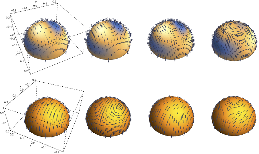
Figure 6: The direction of the perturbed magnetic field, plotted along a series of hemispherical shells beginning near the centre and ending near the surface. From left to right, the shells represent $r/R_{*}=0.2,0.4,0.6,0.8$ respectively. The upper row of plots shows the unit poloidal vector and the lower row the unit toroidal vector. Since arrows into and out of contours are hard to distinguish, we use colour coding for the strength of the radial field component: blue represents a region of field lines pointing towards the centre of the star, whilst white indicates outward-pointing field lines. This only applies to the poloidal-field plots, as toroidal fields are by definition non-radial, and so their arrows are all tangential to the hemispherical shells. Each poloidal/toroidal plot is viewed from the same $(x,y)$ position as in figure 5, but from above – i.e. for a $z>0$ position, unlike the $z<0$ vantage points of figure 5. To save space the axes and bounding box are only drawn for the left-hand plots. Finally, we take $\chi=\pi/16$ for all plots, though there is little variation of the field’s direction with inclination angle.

Having found solutions for $U_{l}$ and $W_{l}$, we may now insert these into equation (172) to find $\delta{\bf B}$. The resulting field configuration is complicated, and we have found it clearest to separate it into its poloidal and toroidal components. First, in figure 5 we plot the magnitudes of these components. Broadly speaking, the perturbed magnetic field is strongest towards the centre, and the toroidal component is about double the strength of the poloidal one. For most values of the inclination angle the $m=1$ component dominates over $m=2$, so the near-aligned ($\chi=\pi/16$) and near-orthogonal ($\chi=7\pi/16$) results are visibly similar. For $\chi=\pi/2$, when the magnetic and rotation axes are orthogonal, there is only an $m=2$ component. However, this situation is actually stationary (and therefore does not correspond to precession); from equation (7) we see that $\omega=0$ for $\chi=\pi/2$, and consequently (by equation (201)), $\partial(Y_{l}^{m}(\theta,\lambda))/\partial t=0$.

Next, we show the direction of the magnetic field, in figure 6. The clearest visualisation we could find was to plot the poloidal and toroidal unit vectors over a nested sequence of constant-radius shells with $r/R_{*}=0.2,0.4,0.6$ and $0.8$. Comparing the field across consecutive shells should, hopefully, allow the reader to visualise the full 3-dimensional field-line structure. The toroidal component is clearer, since (by definition) its field lines run along constant-$r$ shells. For the poloidal component, note that the blue and white patches are in roughly the same position on each contour, meaning that a given field line moves towards the centre of the star through the blue regions, then bends back and comes out through a neighbouring white region to its ‘starting’ location, thus forming a closed loop (as dictated by the requirement that $\nabla\cdot\delta{\bf B}=0$).

7.4 $\mn@boldsymbol{\xi}$-motions

\psfrag{chi=1/16}{$\chi=\displaystyle{\frac{\pi}{16}}$}\psfrag{chi=7/16}{$\chi=\displaystyle{\frac{7\pi}{16}}$}\psfrag{chi=1/2}{$\chi=\displaystyle{\frac{\pi}{2}}$}\psfrag{Bpol}{$|\delta{\bf B}_{\textrm{pol}}|$}\psfrag{Btor}{$|\delta{\bf B}_{\textrm{tor}}|$}\includegraphics[width=433.62pt]{paper_figs/xi_cont.eps}

Figure 7: 3-dimensional contour plots showing the magnitude of $\dot{\mn@boldsymbol{\xi}}$, for $\chi=\pi/16$ (left) and $\chi=7\pi/16$ (right). The details are the same as for figure 5, except that each contour represents a value $\sqrt{2}$ times that of the last, meaning that the innermost contour has twice the value of the outermost.

At last we come to the $\mn@boldsymbol{\xi}$-motions: the non-rigid velocity field present in a precessing fluid star, and the original goal of this paper. We recall that these may now be calculated from our solutions $\bar{U}_{l},X_{l}$ using equations (219)-(221). As for $\delta{\bf B}$, we separate the information about $\dot{\mn@boldsymbol{\xi}}$ into two figures, one showing the magnitude of $\dot{\mn@boldsymbol{\xi}}$ and the other its direction. The contours of $\dot{\mn@boldsymbol{\xi}}$, shown in figure 7, represent smaller differences than those used above for $\delta{\bf B}$ – the speed $|\dot{\mn@boldsymbol{\xi}}|$ only differs by a factor of $\sqrt{2}$ between neighbouring contours, and therefore only varies by a factor of two across most of the stellar interior. Like the perturbed toroidal field from the lower panels in figure 5, the speed is greatest in a torus centred on the origin and aligned along the $x=0$ plane. For the near-aligned case ($\chi=\pi/16$) $\dot{\mn@boldsymbol{\xi}}$ is approximately reflection symmetric about the $x=0$ plane, but as the inclination angle is increased the speed lowers more quickly in the $x<0$ region ($\chi=7\pi/16$ plot). Finally, as mentioned in the previous subsection, $\dot{\mn@boldsymbol{\xi}}={\bf 0}$ for the limiting case of $\chi=\pi/2$.

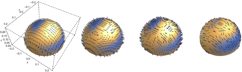
Figure 8: The direction of the $\dot{\mn@boldsymbol{\xi}}$ vector field on constant-radius shells of $r/R_{*}=0.2,0.4,0.6$ and $0.8$ (left to right), for $\chi=\pi/16$. See the caption of figure 6 for details.

The direction of $\dot{\mn@boldsymbol{\xi}}$ is shown in figure 8. Close to the centre and to the outer boundary, the velocity is roughly tangential to constant-$r$ shells, but in between it has a large radial component. As for the poloidal-field direction plots, the blue and white patches are in the same location for each of the four shells in figure 8, meaning that there is a meridional circulation of fluid, with streamlines moving towards the centre of the star through the blue regions and back out through the white regions. Unlike the magnetic-field case, however, these streamlines do not need to close, since $\nabla\cdot\dot{\mn@boldsymbol{\xi}}\neq 0$ (i.e. the flow is compressible). Not restricting to incompressible flow was, in fact, the place at which our approach first diverged from that of Mestel & Takhar (1972); recall the discussion of section 2. For this reason, it is logical to close this section by looking at the behaviour of $\nabla\cdot\dot{\mn@boldsymbol{\xi}}$ itself.

\psfrag{divxi}{$\displaystyle{\frac{r\nabla\cdot\dot{\mn@boldsymbol{\xi}}}{|\dot{\mn@boldsymbol{\xi}}|}}$}\psfrag{r}{$\hat{r}$}\psfrag{th=pi8}{$\theta=\pi/8$}\psfrag{th=pi4}{$\theta=\pi/4$}\psfrag{th=3pi8}{$\theta=3\pi/8$}\includegraphics[width=433.62pt]{paper_figs/divxi.eps}

Figure 9: Divergence of $\dot{\mn@boldsymbol{\xi}}$, normalised by the speed $|\dot{\mn@boldsymbol{\xi}}|$ divided by the radius, to make a dimensionless quantity. We show the behaviour of this quantity for $\lambda=\pi/2$ and three values of $\theta$, as labelled. This plot demonstates that for barotropic stellar models, the higher-order motions in a precessing fluid star are in fact highly compressible. It also gives an idea of how strong buoyancy forces would need to be in order to produce the incompressible motions discussed in Mestel & Takhar (1972).

In figure 9 we plot the divergence of $\nabla\cdot\dot{\mn@boldsymbol{\xi}}$, normalised by $|\dot{\mn@boldsymbol{\xi}}|/r$ to give a dimensionless quantity. In a barotropic star one cannot assume incompressible motions, and indeed we see that $\nabla\cdot\dot{\mn@boldsymbol{\xi}}$ deviates greatly from zero, especially in the outer regions. Thermal- or composition-gradient stratification in real stars would provide some additional buoyancy force to suppress compressible motions, but for a given model one still needs to account for such a buoyancy force consistently, and to verify it is sufficiently strong to impose $\nabla\cdot\dot{\mn@boldsymbol{\xi}}=0$. Figure 9 gives an idea of how and where such forces would have to act to ensure $\nabla\cdot\dot{\mn@boldsymbol{\xi}}=0$.

8 Discussion

This paper has been concerned with a detailed description of the dynamics of a rotating magnetised star, in the general ‘oblique rotator’ case when the magnetic and rotational axes are misaligned by some angle $0<\chi<\pi/2$. The star’s bulk motion is that of free precession, but sustaining this in a fluid star requires additional dynamics in the interior: time-dependent velocity and magnetic fields. The concept of non-rigid precession was first described by Mestel & Takhar (1972), who produced simplified models of the perturbed field $\dot{\mn@boldsymbol{\xi}}$ using first-order perturbation equations. A new calculation of $\dot{\mn@boldsymbol{\xi}}$ was presented in Mestel et al. (1981), who also used this, in turn, to calculate magnetic field perturbations, given a poloidal background field. Nittmann & Wood (1981) performed the same analysis for a toroidal background field.

In this paper we argue that a consistent solution for both $\dot{\mn@boldsymbol{\xi}}$ and $\delta{\bf B}$ can only come from solving a higher-order set of equations than those previously considered. A large part of the work presented here involves a detailed formalism to describe these perturbations (section 3), algebraic manipulation to reduce them to a set of differential equations in radial functions (section 5), and then solving these (section 7 and appendix B).

In order to make the problem tractable, we have had to make a number of assumptions, and now need to consider how these affect the validity of our model when applied to different classes of star. Nonetheless, we emphasise that our model contains the minimum essential physics for non-rigid precession, and so everything that follows concerns additional effects. Even when our assumptions are unjustifiable, then, the work presented here can be regarded as a ‘background’ model upon which to build.

The most major simplification we have made is assuming a toroidal background magnetic field. Purely toroidal fields, like purely poloidal fields, suffer rapidly-growing dynamical instabilities – and so cannot be realistic models of stellar magnetic fields (Tayler, 1973), which must instead feature both poloidal and toroidal components. However, in the absence of an additional stabilising mechanism, there are indications that even mixed poloidal-toroidal fields are generically unstable (Lander & Jones, 2012; Mitchell et al., 2015). On the other hand, toroidal-dominated stable equilibria have been found for stellar models with an additional thermal-buoyancy force (Braithwaite, 2009). The issue of stable magnetic equilibria is not fully settled, but if the toroidal component is generically the dominant one in stars, our results may indeed be a reasonable first approximation to their precessional dynamics.

For a stellar model with a purely poloidal field, we believe an analogous analysis to ours could be carried out. However, whilst a toroidal field has a component only in the direction of one spherical-polar coordinate (the azimuthal one, $\lambda$), a poloidal field’s depends on the other two ($r$ and $\theta$), suggesting that spherical-polar coordinates will not be appropriate for studying this problem. Instead, one can work in a coordinate system fitted to poloidal-field lines (Bernstein et al., 1958), in which case all the steps of our toroidal-field calculation should be tractable for a poloidal field too. There is, however, no coordinate system in which a mixed poloidal-toroidal field becomes similarly simple (see, e.g., Tayler (1980)); for a stellar model with such a background field, it seems inevitable that a fully numerical approach would be required.

Neutron stars: most of the assumptions made in this paper are typical ones in the context of neutron-star modelling. This is certainly not equivalent to saying that they are all justifiable on physical grounds, however, so each needs further attention. The $\gamma=2$ polytrope we adopt is quite suitable for a single-fluid model of a neutron star, but the cores of mature neutron stars are better described by a two-fluid equation of state in which the neutrons are superfluid; simple magnetic equilibrium models for mature neutron-star cores may be found in which each fluid component obeys its own polytropic relation (Lander, Andersson & Glampedakis, 2012; Glampedakis, Andersson & Lander, 2012). The neutron superfluid will decouple from the precessional dynamics we consider in this paper, and so only the charged component is relevant. This component is, however, better described by a polytropic index $\gamma\approx 3/2$.

It is reasonable to assume that no additional buoyancy forces enter the precessional dynamics of a mature neutron star. A neutron star in equilibrium has a density-dependent fraction of neutrons to protons. When the neutrons are not superfluid, displacing a fluid element results in chemical reactions which convert between neutrons and protons to restore the equilibrium fraction of protons and neutrons, and this represents a buoyancy force associated with the composition-gradient stratification (Reisenegger & Goldreich, 1992). However, these reactions are strongly suppressed (along with the associated buoyancy) when the neutrons are superfluid. In addition, neutron stars become isothermal very early on in their life, so there is negligible thermal-gradient stratification. Finally, we have already argued (in section 5.7) that crustal elasticity and the matching between crust and core could seriously modify our solutions in the outermost region, $0.9R_{*}\leq r\leq R_{*}$, and so we considered it wisest to exclude this region altogether, and place the outer boundary for our solutions at a radius of $0.9R_{*}$.

The most significant neutron-star physics we have failed to account for is the superconducting nature of the stellar core. Since most of this region is believed to form a type-II superconductor, however, the magnetic field will still penetrate the core and produce a macroscopically uniform magnetic force (Baym, Pethick & Pines, 1969). The conceptual picture should thus remain intact: the magnetic field lends rigidity to the fluid, inducing bulk precession but at the expense of requiring additional internal motions and magnetic-field perturbations. Quantitatively, however, the nature of these perturbations will undoubtedly be different – and qualitatively we would expect them to scale with the superconducting magnetic force $\propto H_{c1}B\sim 10^{15}B$ instead of the normal Lorentz force $\propto B^{2}$ (Easson & Pethick, 1977; Wasserman, 2003).

The velocity field $\dot{\mn@boldsymbol{\xi}}$ represents a ‘macroscopic’ coupling between the star’s rotation and magnetic field. In a neutron-star core with type-II superconducting protons and superfluid neutrons, however, there is a competing ‘microscopic’ coupling mechanism: the interaction of rotational neutron vortices with magnetic proton fluxtubes (Ruderman, Zhu & Chen, 1998; Link, 2003). Ascertaining the relative importance of these two mechanisms would be an important step towards a quantitative picture of non-rigid neutron-star precession.

White dwarfs: unlike neutron stars, white dwarfs form a broad class of stars, with differences in chemical composition and the physics governing their different regions. The major subdivision of white dwarfs of relevance to this paper is between the magnetic and non-magnetic white dwarfs. Like neutron stars, magnetic white dwarfs have field strengths spanning several orders of magnitude, but with an upper limit of $\lesssim 10^{9}$ G. Many of these strongly magnetised objects have, like magnetars, long rotation periods, although there are some rapidly-rotating and highly-magnetised white dwarfs (Ferrario, de Martino & Gänsicke, 2015) – the ideal combination for relatively short precession periods.

The equation of state for a white dwarf is a degenerate Fermi gas. In the high-density limit this reduces to a $\gamma=4/3$ polytrope, and in the low-density limit to a $\gamma=5/3$ polytrope (Nauenberg, 1972). For lower densities then, the $\gamma=2$ relation adopted here is probably not an egregious approximation to white-dwarf matter. Imposing an outer boundary below the surface is also justifiable, since the degenerate core of white dwarfs gives way abruptly to a low-mass nondegenerate envelope region – although the envelope is only $\sim 30$km (Althaus et al., 2010), meaning that a more appropriate radius to impose the outer boundary at would be $\sim 0.997R_{*}$ (taking care that the perturbative scheme is still applicable at this radius; see section 5.6).

In this work we have assumed a fluid region which extends to the stellar centre, which is not always the case for white dwarfs: as they become older and colder, white dwarfs begin to form solid cores (Van Horn, 1968), with the crystallisation proceeding from the centre outwards and solidifying the whole star over a timescale of $\sim 10^{9}$ yr (Iben & Tutukov, 1984). Elasticity will then affect the induced velocity and magnetic-field perturbations in the solid core; for a sufficiently rigid core lattice these perturbations would become negligible, and the core’s motion would then be well described by standard rigid-body free precession. Finally, more detailed modelling of white-dwarf precession should account for the fact that these stars are non-barotropic, with stratification due to both composition and thermal gradients.

Nondegenerate (main-sequence) stars: with some caveats, our analysis applies to objects along the upper part of the main sequence of nondegenerate stars. Upper-main-sequence stars have higher masses and more simple field topologies than other nondegenerate stars, and since their envelopes appear to be in radiative equilibrium (rather than convective), dynamo action seems unlikely. The conclusion is that the magnetic fields in these envelopes are likely to be in dynamically stable equilibrium states. Of these stars, the most highly magnetised are the chemically peculiar A and B-type stars, with field strengths up to $\sim 10^{4}$ G. Upper-main-sequence stars with strong magnetic fields tend to rotate far more slowly than their weakly-magnetised counterparts, such as the normal A and B stars (Donati & Landstreet, 2009).

In the radiative envelopes of main-sequence stars our analysis is broadly applicable, but as for white dwarfs should be modified by the inclusion of a thermal buoyancy force. This will constrain the form of $\dot{\mn@boldsymbol{\xi}}$ and $\delta{\bf B}$, but in a way which can only be confirmed by including thermal effects in a self-consistent matter in the whole analysis. As for partially-crystallised white dwarfs, our analysis will not be valid all the way to the centre of main-sequence stars. In this case the reason is the presence of an inner core region where vigorous convection disrupts and regenerates the magnetic field – and so our assumption of a large-scale stable background magnetic field becomes invalid here. Moving to the outer boundary, there is no distinct outer region of the radiative zone where one would expect the $\mn@boldsymbol{\xi}$-motions to stop. Our approach requires us to cut off the solution before reaching the stellar surface $R_{*}$ (see section 5.6), but as long as we choose an outer boundary close to $R_{*}$ we will only be neglecting a small, low-density region of the star.

For all classes of star, the internal velocity and magnetic fields solved for in this paper may have significant effects on their evolution and dynamics. In particular, since they couple the star’s rotation and magnetic fields, the dissipation of these motions could cause the evolution of the inclination angle (Spitzer, 1958). For toroidal fields, the case considered here, the dissipation will tend to cause the star to become an orthogonal rotator, $\chi\to\pi/2$; for poloidal fields $\chi\to 0$ (Mestel & Takhar, 1972). For the more realistic case of mixed poloidal-toroidal fields the evolution of $\chi$ will be dictated by the dominant field component, and so observations of this evolution could allow one to infer details of the star’s internal magnetic field. Although we do not intend to tackle a fully self-consistent evolution of dissipative processes, a qualitative discussion of this and applications to astrophysics will be presented in a follow-up paper.

9 Summary

We have presented a formalism and solution method for models of rotating magnetic stars with misaligned rotation and magnetic axes – sometimes known as oblique rotators. We began with arguably the simplest necessary pieces of physics to describe this problem: a rigid primary rotation of the star, and a large-scale $m=0$ dipolar toroidal magnetic field. Despite this simplicity, we have found that the dynamics of such stars involve internal velocity and magnetic-field perturbations with highly complex geometries. The perturbed velocity and magnetic field are both stronger towards the centre of the star, and the toroidal perturbed field is a factor of two more intense than the poloidal. There are indications that whilst the perturbed toroidal field is dominated by its dipole ($l=1$) piece, the poloidal component of the magnetic-field perturbation may have significant contributions from many higher multipoles – and in fact its $l=4$ component is stronger than its lowest-order multipole, a quadrupole ($l=2$) piece. The velocity field has significant azimuthal and meridional components, and deviates strongly from being solenoidal – i.e., the internal motions are highly compressible. The secular dissipation of these perturbations will cause the star to evolve over time into either an aligned or orthogonal rotator, and so the distribution of inclination angles in stars is likely to be connected with their internal magnetic fields.

Appendix A Spherical-harmonic decompositions of source terms

Since we solve equations for a given $m$, we need the source terms decomposed into $Y_{l}^{m}$ pieces too. We use the following relations between trigonometric functions and spherical harmonics $Y_{l}^{m}(\theta,\lambda)$:

$$\sin(\theta)\sin\lambda =i\sqrt{\frac{2\pi}{3}}(Y_{1}^{1}+Y_{1}^{-1}),$$ (232)

$$\sin^{2}\theta\sin(2\theta)\cos\lambda =\frac{8}{21}\sqrt{\frac{\pi}{5}}(Y_{4}^{1}-Y_{4}^{-1})-\frac{8}{7}\sqrt{\frac{2\pi}{15}}(Y_{2}^{1}-Y_{2}^{-1}),$$ (233)

$$\sin^{4}\theta\cos(2\lambda) =-\frac{4}{21}\sqrt{\frac{2\pi}{5}}(Y_{4}^{2}+Y_{4}^{-2})+\frac{4}{7}\sqrt{\frac{6\pi}{5}}(Y_{2}^{2}+Y_{2}^{-2}),$$ (234)

together with those given in equations (76), (77), (118) and (119). These allow us to decompose the scalar functions $\Upsilon_{\delta\mathcal{L}}$ and $\Psi_{\delta\mathcal{L}}$ from equations (132) and (133), which enter as source terms in our final system of equations:

$$\Upsilon_{\delta\mathcal{L}}=\frac{i\alpha^{2}\Lambda^{2}r}{16G}\sqrt{\frac{\pi}{6}}\left\{\sin(2\chi)\left[j_{2}({\textstyle{\frac{\pi r}{R_{*}}}})-16k_{B}\right](Y_{1}^{1}+Y_{1}^{-1})+\frac{1}{3\sqrt{7}}j_{2}({\textstyle{\frac{\pi r}{R_{*}}}})\left[\sqrt{2}\sin(2\chi)(Y_{3}^{1}+Y_{3}^{-1})-\sqrt{5}\sin^{2}\chi(Y_{3}^{2}-Y_{3}^{-2})\right]\right\}$$ (235)

and

$$\Psi_{\delta\mathcal{L}}=\frac{\alpha^{2}\Lambda^{2}}{336G}\sqrt{\frac{5\pi}{6}} \bigg{\{}-\sin(2\chi)\left[{\textstyle{\frac{\pi r}{R_{*}}}}j_{1}({\textstyle{\frac{\pi r}{R_{*}}}})+11j_{2}({\textstyle{\frac{\pi r}{R_{*}}}})+12{\textstyle{\frac{\pi r}{R_{*}}}}\cot({\textstyle{\frac{\pi r}{R_{*}}}})j_{2}({\textstyle{\frac{\pi r}{R_{*}}}})\right](Y_{2}^{1}-Y_{2}^{-1})$$

$$\ \ \ \ +\sin^{2}\chi\left[-2{\textstyle{\frac{\pi r}{R_{*}}}}j_{1}({\textstyle{\frac{\pi r}{R_{*}}}})+20j_{2}({\textstyle{\frac{\pi r}{R_{*}}}})+18{\textstyle{\frac{\pi r}{R_{*}}}}\cot({\textstyle{\frac{\pi r}{R_{*}}}})j_{2}({\textstyle{\frac{\pi r}{R_{*}}}})\right](Y_{2}^{2}+Y_{2}^{-2})$$

$$\ \ \ \ +\sqrt{6}\sin(2\chi)\left[-{\textstyle{\frac{\pi r}{R_{*}}}}j_{1}({\textstyle{\frac{\pi r}{R_{*}}}})+3j_{2}({\textstyle{\frac{\pi r}{R_{*}}}})+2{\textstyle{\frac{\pi r}{R_{*}}}}\cot({\textstyle{\frac{\pi r}{R_{*}}}})j_{2}\right](Y_{4}^{1}-Y_{4}^{-1})$$

$$\ \ \ \ -\sqrt{3}\sin^{2}\chi\left[-{\textstyle{\frac{\pi r}{R_{*}}}}j_{1}({\textstyle{\frac{\pi r}{R_{*}}}})+3j_{2}({\textstyle{\frac{\pi r}{R_{*}}}})+2{\textstyle{\frac{\pi r}{R_{*}}}}\cot({\textstyle{\frac{\pi r}{R_{*}}}})j_{2}\right](Y_{4}^{2}+Y_{4}^{-2})\bigg{\}}.$$ (236)

Appendix B Numerical solution and error estimation

We use the NDSolve command in the software package Mathematica in order to solve our system of equations. NDSolve is not capable of solving differential-algebraic equations as boundary-value problems, as we would need, so we instead convert our original equations into a system of ODEs by working with equation (164) and equation (174). We implement the boundary conditions as summarised in table 2. The full solution to our precession problem should be an infinite sum of harmonics, but we terminate at a value of $l_{\textrm{max}}=4$, as we have failed to find a successful method of solving the equations for arbitrary truncation values; implementation of the techniques of section 5.4 to $l_{\textrm{max}}>4$ typically results in a solution which does not satisfy the the highest-$l$ equation to acceptable accuracy. Finally, we non-dimensionalise the variables in our equations by suitable combinations of $G,\rho_{c}$ and $R_{*}$ (these three quantities contain instances of mass, length and time, so together they may be used to non-dimensionalise any other quantity). This allows us to work with quantities whose magnitude does not deviate excessively from unity, unlike the unwieldy physical parameters for stellar models. It also allows one to scale results easily to parameters appropriate for models of main-sequence stars, white dwarfs and neutron stars.

The problems discussed up to this point have been mathematical in origin, but the numerical solution has also required some care. We have found that the numerical algorithm typically requires 25-digit precision or higher for success. Finally, Mathematica returns zero-divided-by-zero errors with the equations in their original form. To avoid these, certain quantities need to be evaluated at a point slightly displaced from the centre. To minimise the introduced error, and to prevent it from affecting conditions at the outer boundary (the crust-core boundary), we define the function

$$\mathcal{D}(r)\equiv\mathfrak{d}(r-R_{\textrm{out}}),$$ (237)

where $\mathfrak{d}$ is some small constant, and in the equations in the Mathematica notebook we make the replacement $r\mapsto r+\mathcal{D}(r)$ in the quantities $rU^{\prime}_{l}(r),\Upsilon^{\prime}_{l}(r),(r\rho^{\prime}_{0}/\rho_{0})^{\prime}$. At the end of this section, we verify that the introduced error is small, and converges to zero as $\mathfrak{d}\to 0$.

B.1 Verification of DAE solution method

In section 5.4, we presented a method to solve the system of DAEs (164) and (165). We differentiated the second of these DAEs in order to get a system of ODEs, (164) and (174); however, the set of solutions to these ODEs is larger than the set of solutions to the original DAEs, and so a typical solution to the ODEs would differ from a solution to the DAEs by some ‘integration constant’ factor. The method of section 5.4 was designed to pick out the correct integration constant, so let us now check that our solutions do indeed satisfy the original DAEs.

Table 3: An example set of superficially sensible boundary conditions on the ODE system (164) and (174), which are nonetheless not acceptable, as they do not ensure the resulting solution is also a solution of the original DAEs (164) and (165).

$m$	centre	crust-core boundary
	$\bar{U}^{\prime}_{2}(0)=0$	$R_{\textrm{out}}\bar{U}^{\prime}_{2}(R_{\textrm{out}})+4\bar{U}_{2}(R_{\textrm{out}})=0$
1	$\bar{U}_{4}^{\prime}(0)=0$	$R_{\textrm{out}}\bar{U}^{\prime}_{4}(R_{\textrm{out}})+6\bar{U}_{4}(R_{\textrm{out}})=0$
		$X_{1}(R_{\textrm{out}})=0$
		$X_{3}(R_{\textrm{out}})=0$
	$\bar{U}^{\prime}_{2}(0)=0$	$R_{\textrm{out}}\bar{U}^{\prime}_{2}(R_{\textrm{out}})+4\bar{U}_{2}(R_{\textrm{out}})=0$
2	$\bar{U}_{4}^{\prime}(0)=0$	$R_{\textrm{out}}\bar{U}^{\prime}_{4}(R_{\textrm{out}})+6\bar{U}_{4}(R_{\textrm{out}})=0$
		–
		$X_{3}(R_{\textrm{out}})=0$

We substitute our numerical solution $\mathcal{S}\equiv\{X_{l},\bar{U}_{l}\}$ back into equations (164) and (165). To produce a normalised error estimate, we recall that the $X_{l}$ functions are only non-zero for odd $l$, and the $\bar{U}_{l}$ functions are non-zero for even $l$. Since we solve (165) (in differentiated form) for odd $l$ and (164) for even $l$, this means that for a particular value of $l$, we can associate one equation with one particular function, e.g. equation (165) for $l=1$ may be associated with $X_{1}$. We produce normalised errors $\mathfrak{e}_{l}(r)$ using this observation:

$$\mathfrak{e}_{l}(r)\equiv\begin{cases}\displaystyle{\frac{\textrm{$\mathcal{S}$ substituted into equation \eqref{DAE1}}}{\max{(\bar{U}_{l})}}\textrm{ (for even $l$)}},\\ \displaystyle{\frac{\textrm{$\mathcal{S}$ substituted into equation \eqref{DAE2}}}{\max{(X_{l})}}\textrm{ (for odd $l$)}}.\end{cases}$$ (238)

In figure 10 we show the resulting errors, whose small size indicate we have successfully obtained a solution to the DAE system. For comparison, we also perform a consistency check by substituting the solution back into the ODEs (164) and (174); since these were the equations actually solved by Mathematica, the resulting error is very small.

\psfrag{Mathematica error}{Inherent Mathematica error}\psfrag{integration-const error}{\ \ \ Boundary conditions from table \ref{wrongBCs}}\psfrag{error removed}{\ \ \ Boundary conditions from table \ref{BCs}}\psfrag{e1}{$\mathfrak{e}_{1}$}\psfrag{e2}{$\mathfrak{e}_{2}$}\psfrag{e3}{$\mathfrak{e}_{3}$}\psfrag{e4}{$\mathfrak{e}_{4}$}\psfrag{r}{$\hat{r}$}\includegraphics[width=433.62pt]{paper_figs/error-plots.eps}

Figure 10: Comparison of errors $\mathfrak{e}_{l}$ (see equation (238)) for different boundary conditions. We convert our original differential-algebraic equations (164) and (165) into ODEs which Mathematica is capable of solving by differentiating the latter equation, giving equation (174). The left-hand plots show the result of subsituting the obtained solution back into (164) and (174); this is merely a consistency check of Mathematica’s algorithm, and the resulting error is predictably small (regardless of which set of boundary conditions we use). We then solve (164) and (174) together with a naïve set of boundary conditions, table 3, which do not contain information about the original DAEs. We substitute the solution obtained with these boundary conditions back into the original DAEs, (164) and (165), and show the resulting error in the central plots. For the lower of these plots, corresponding to the equation which was differentiated, a large, constant error can be seen. This reflects the fact that a solution to (174) will typically differ by some integration constant from a solution of the original equation (165). To fix this constant at the correct value (of zero), we need to use the more careful boundary conditions of table 2. With these, as shown in the right-hand plots, the error becomes small.

If we had not worried about fixing the integration constant correctly, we might instead have adopted a set of boundary conditions like those of table 3, which are natural-looking ones to use to ensure that solutions are well-behaved at the centre and do not give rise to a current sheet at the outer boundary. Figure 10 clearly shows that the resulting solutions fail to satisfy the original DAE system.

B.2 Convergence

To prevent numerical errors at the centre, we evaluated some quantities at a small radial distance – given by equation (237) – from their correct location. Our final check is to make sure the introduced error is small, and converges to zero in the limit $\mathfrak{d}\to 0$; we do this in figure 11. Here we have used the correct boundary conditions, from table 2; note that the large ‘integration constant’ error resulting from using the boundary conditions of table 3 does not converge away as $\mathfrak{d}\to 0$.

\psfrag{frakd-3}{$\mathfrak{d}=10^{-3}$}\psfrag{frakd-4}{$\mathfrak{d}=10^{-4}$}\psfrag{frakd-5}{$\mathfrak{d}=10^{-5}$}\psfrag{e1}{$\mathfrak{e}_{1}$}\psfrag{e2}{$\mathfrak{e}_{2}$}\psfrag{e3}{$\mathfrak{e}_{3}$}\psfrag{e4}{$\mathfrak{e}_{4}$}\psfrag{r}{$\hat{r}$}\includegraphics[width=433.62pt]{paper_figs/frakd-conv.eps}

Figure 11: Convergence of the error in solutions as $\mathfrak{d}\to 0$. For $\mathfrak{d}=10^{-5}$, the noisy inherent error present from Mathematica’s solution becomes visible; i.e. the error introduced from evaluating quantities slightly away from the origin reduces to the level of intrinsic error from Mathematica’s solution method. Note that the actual physical results for $\bar{U}_{l},X_{l}$ for these three values of $\mathfrak{d}$ are indistinguishable.

References

- Althaus et al. (2010) Althaus L.G., Córsico A.H., Isern J., García-Berro E., 2010, Astron. Astrophys. Rev., 18, 471
- Arfken & Weber (2005) Arfken G.B., Weber H.J., 2005, Mathematical Methods for Physicists, Elsevier Academic Press, Oxford
- Backus (1986) Backus G., 1986, Rev. Geophys., 24, 75
- Baym, Pethick & Pines (1969) Baym G., Pethick C., Pines D., 1969, Nature, 224, 673
- Bernstein et al. (1958) Bernstein I.B., Frieman E.A., Kruskal M.D., Kulsrud R.M., 1958, Proc. Royal Soc. London, 244, 17
- Braithwaite (2009) Braithwaite J., 2009, MNRAS, 397, 763
- Chandrasekhar (1939) Chandrasekhar S., 1939, An Introduction to the Study of Stellar Structure, University of Chicago Press, Chicago
- Chandrasekhar & Fermi (1953) Chandrasekhar S., Fermi E., 1953, ApJ, 118, 116
- Chandrasekhar & Prendergast (1956) Chandrasekhar S., Prendergast K.H., 1956, PNAS, 42, 5
- Ciolfi et al. (2009) Ciolfi R., Ferrari V., Gualtieri L., Pons J.A., 2009, MNRAS, 397, 913
- Dall’Osso, Shore & Stella (2009) Dall’Osso S., Shore S.N., Stella L., 2009, MNRAS, 398, 1869
- Donati et al. (2002) Donati J.-F., Babel J., Harries T.J., Howarth I.D., Petit P., Semel M., 2002, MNRAS, 333, 55
- Donati & Landstreet (2009) Donati J.-F., Landstreet J.D., 2009, Annu. Rev. Astron. Astrophys., 47, 333
- Easson & Pethick (1977) Easson I., Pethick C.J., 1977, PRD, 16, 275