Rapidly convergent quasi-periodic Green functions for scattering by arrays of cylinders—including Wood anomalies

Abstract

This paper presents a full-spectrum Green function methodology (which is valid, in particular, at and around Wood-anomaly frequencies) for evaluation of scattering by periodic arrays of cylinders of arbitrary cross section—with application to wire gratings, particle arrays and reflectarrays and, indeed, general arrays of conducting or dielectric bounded obstacles under both TE and TM polarized illumination. The proposed method, which, for definiteness is demonstrated here for arrays of perfectly conducting particles under TE polarization, is based on use of the shifted Green-function method introduced in the recent contribution (Bruno and Delourme, Jour. Computat. Phys. pp. 262–290 (2014)). A certain infinite term arises at Wood anomalies for the cylinder-array problems considered here that is not present in the previous rough-surface case. As shown in this paper, these infinite terms can be treated via an application of ideas related to the Woodbury-Sherman-Morrison formulae. The resulting approach, which is applicable to general arrays of obstacles even at and around Wood-anomaly frequencies, exhibits fast convergence and high accuracies. For example, a few hundreds of milliseconds suffice for the proposed approach to evaluate solutions throughout the resonance region (wavelengths comparable to the period and cylinder sizes) with full single-precision accuracy.

1 Introduction

We consider the problem of scattering of a monochromatic plane wave by a periodic array of cylinders of general cross section. We approach this problem by means of the methodology introduced in [7] which, based on use of a certain shifted Green function, provides a solver for problems of scattering by periodic surfaces which is valid and accurate throughout the spectrum—including Wood frequencies [30, 33], at which the classical quasi-periodic Green function ceases to exist

A variety of approaches have been used to tackle this important problem including, notably, methods based on use of integral equations; cf. [2, 3, 7, 8, 9] and references therein. The success of the integral-equation approach results from its inherent dimensionality reduction (only the boundary of the domain needs to be discretized) and associated automatic enforcement of radiation conditions.

For the sake of simplicity the methodology presented in this article assumes perfectly conducting obstacles under TE polarization. The method can be easily extended to TM polarization and dielectric cylinders: the dielectric case does not give rise to additional difficulties, and the hyper-singular operators that arise in the TM case of polarization can be handled by means of existing regularization techniques (see e.g. [6] and references therein). The main strategy developed in the present paper can thus be applied in those contexts without significant modifications.

As is well known, classical expansions for quasi-periodic Green functions converge extremely slowly, and they of course completely fail to converge at Wood anomalies. A number of methods have been introduced to tackle the slow-convergence difficulty, including the well known Ewald summation method for two and three dimensional problems [1, 12, 19, 20] and many other contributions [13, 14, 16, 22, 24, 25, 26]. Unfortunately, however, none of these methods resolve the difficulties posed by Wood anomalies. Recently, a new quasi-periodic Green function was introduced [7] for the problem of scattering by periodic surfaces which, relying on use of certain linear combinations of shifted free-space Green functions (which amount to discrete finite-differencing of the Green functions) can be used to produce arbitrary (user-prescribed) algebraic convergence order for frequencies throughout the spectrum, including Wood frequencies [30, 33].

A straightforward application of this procedure leads to an operator equation that contains denominators which tend to zero as a Wood anomaly is approached. To remedy this situation a strategy based on use of the Woodbury-Sherman-Morrison formulae is introduced which completely regularizes the problem and provides a limiting solution as Wood frequencies are approached. To our knowledge, this is the first approach ever presented that is applicable to problems of scattering by periodic arrays of bounded obstacles at Wood anomalies on the basis of quasi-periodic Green functions. It is worth mentioning that an alternative method, not based on the use of quasi-periodic Green functions and which is also applicable at Wood anomalies, was proposed in [2, 3]. In that approach, whose generalization to corresponding three-dimensional problems at Wood anomalies has not been provided, the quasi-periodicity is enforced through use of auxiliary layer potentials on the boundaries of the periodic cell. As suggested by the treatment [5] for the problem of scattering by bi-periodic surfaces in three-dimensions, the shifted Green function approach can be extended to three-dimensional problems without difficulty.

In order to demonstrate the character of the new approach we present numerical methods based on use of a combination of three main elements: the half-space quasi-periodic Green function, the smooth windowing methodology [5, 7, 23] (which gives rise to super-algebraically fast convergence away from Wood anomalies) and high-order quadratures for singular integrals [15, 17, 21, 32]. As shown by means of a variety of numerical results, highly accurate solvers result from this strategy—even at and around Wood anomalies. As can be seen in Section 6 the present approach can solve the complete scattering problem for scatterers of arbitrary shape even at anomalous configurations, in fast computing times.

The remainder of this article is organized as follows. Section 2 presents necessary background on the problem of scattering by periodic media. Section 3 summarizes the convergence properties of the shifted quasi-periodic Green function approximation introduced in [7], and Section 4 then presents an associated integral-equation formulation for the solution of the problem of wave scattering by a periodic array of bounded obstacles at all frequencies. The actual numerical implementation we propose, which relies, in addition, on the aforementioned smooth windowing methodology, is presented in Section 5 (the super-algebraic convergence of the smooth windowing methodology at non-anomalous configurations has been established in [5] for bi-periodic structures in three dimensional space; the same ideas can be applied to establish the result for a linear periodic array in two-dimensional case). Section 6, finally, presents a variety of numerical results demonstrating the properties of the overall approach.

2 Preliminaries

2.1 Scattering by a periodic array of bounded obstacles

We consider problems of scattering by a one-dimensional perfectly-conducting diffraction grating of period $L$ ($L>0$) in two-dimensional space under TE polarization. The scatterer is assumed to equal a union of the form

$$D=\bigcup_{n=-\infty}^{\infty}D_{n}$$ (1)

of mutually disjoint closed sets $D_{n}$, where $D_{0}$ equals a union of a finite number of non-overlapping connected bounded components, and where $D_{n}=D_{0}+nL\hat{x}$, ($\hat{x}=(1,0)$, $n\in\mathbb{Z}$); see Figure 1. We assume the grating is illuminated by a plane-wave of spatial frequency $k>0$ and incidence angle $\theta$ (measured from the $y$-axis). The scattered wave $u^{\mathrm{s}}$ satisfies the PDE

$$\Delta u^{\mathrm{s}}+k^{2}u^{\mathrm{s}}=0\qquad\mathrm{in}\quad\Omega=\mathbb{R}^{2}\setminus D$$ (2)

along with the condition of radiation at infinity (see Remark 1) and a Dirichlet-type boundary condition:

$$u^{\mathrm{s}}=-u^{\mathrm{inc}}_{k}\quad\mbox{on}\quad\partial D$$ (3)

where, letting $\alpha=k\sin(\theta)$ and $\beta=k\cos(\theta)$ we have set

$$u^{\mathrm{inc}}_{k}(x,y)=e^{i\alpha x-i\beta y}.$$

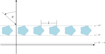
Figure 1: The physical problem: a plane wave with angle of incidence $\theta$ is scattered by an array of cylindrical obstacles distributed periodically in the $x$-direction. The particular star-shaped cylinder cross-section depicted here is given by the parametrization $C(t)=r(t)(\cos(t),\sin(t))\quad\mbox{where}\quad r(t)=1+0.1\cos(5t)+0.01\cos(10t)$.

As is well known, the incoming and scattered waves $u^{\mathrm{inc}}_{k}$ and $u^{\mathrm{s}}$ are $\alpha$ quasi-periodic functions, that is, they satisfy the identities

$$u^{\mathrm{inc}}_{k}(x+nL,y)=e^{i\alpha nL}u_{\mathrm{inc},}(x,y)\quad\mbox{and}\quad u^{\mathrm{s}}(x+nL,y)=e^{i\alpha nL}u^{\mathrm{s}}(x,y).$$

It follows that, assuming

$$D\subset\mathbb{R}\times(M^{-},M^{+})$$ (4)

(see Figure 1) and letting $\alpha_{n}=\alpha+\frac{2\pi}{L}n$, $\beta_{n}^{2}=k^{2}-\alpha_{n}^{2}$, ($\mathrm{Im}(\beta_{n})\geq 0$), the solution $u^{\mathrm{s}}$ admits Rayleigh expansions [28] of the form

$$u^{\mathrm{s}}(x,y)=\sum\limits_{n\in\mathbb{Z}}A_{n}^{\pm}e^{i\alpha_{n}x+i\beta_{n}y}+B_{n}^{\pm}e^{i\alpha_{n}x-i\beta_{n}y}.$$ (5)

Remark 1.

The scattered field consists of a superposition of plane waves that propagate away from $D$ and which remain bounded in the far field; a scattered solution having this property is called radiating. In the present context we impose such a radiation condition by requiring that [28]

$$u^{\mathrm{s}}(x,y)=\sum\limits_{n\in\mathbb{Z}}C_{n}^{+}e^{i\alpha_{n}x+i\beta_{n}y},\quad y>M^{+},\quad\mbox{and}$$ (6)

$$u^{\mathrm{s}}(x,y)=\sum\limits_{n\in\mathbb{Z}}C_{n}^{-}e^{i\alpha_{n}x-i\beta_{n}y},\quad y<M^{-}.$$ (7)

Remark 2.

Throughout this paper $\mathcal{N}$ denotes the finite subset of integers for which $k^{2}-\alpha_{n}^{2}>0$. For $n\in\mathcal{N}$ the functions $e^{i\alpha_{n}x+i\beta_{n}y}$ and $e^{i\alpha_{n}x-i\beta_{n}y}$ are outwardly propagating waves (above and below $D$, respectively). If $k^{2}-\alpha_{n}^{2}<0$, the modes $e^{i\alpha_{n}x+i\beta_{n}y}$ (resp. $e^{i\alpha_{n}x-i\beta_{n}y}$) are evanescent waves, i.e., they decrease exponentially as $y\to+\infty$ (resp. $y\to-\infty$). A scattering setup for which $k^{2}=\alpha_{n_{0}}^{2}$ for some $n_{0}\in\mathbb{Z}$ is called a Wood anomaly configuration and the wavenumber $k$ will be referred as a Wood frequency or Wood anomaly frequency; note that, in such cases the plane wave $e^{i\alpha_{n_{0}}x\pm i\beta_{n_{0}}y}$ travels in directions parallel to the obstacle array. For fixed $L$ and $\theta$ we will consider the set

$$\mathcal{K}_{\mathrm{wa}}=\mathcal{K}_{\mathrm{wa}}(L,\theta)=\{k>0:\,\exists\,n\in\mathbb{Z}\text{ such that }k^{2}=\alpha_{n}^{2}\}$$ (8)

of all Wood frequencies for a given period $L$ and incidence angle $\theta$. Clearly, for each $k_{0}\in\mathcal{K}_{\mathrm{wa}}$ the set

$$\mathcal{N}_{\mathrm{wa}}(k_{0})=\left\{n\in\mathbb{Z}:\beta_{n}(k_{0})=0\right\}$$ (9)

has at least one and at most two elements: either $\mathcal{N}_{\mathrm{wa}}=\{n_{1}\}$ or $\mathcal{N}_{\mathrm{wa}}=\{n_{1},n_{2}\}$. For conciseness, throughout this paper we will write $\mathcal{N}_{\mathrm{wa}}=\{n_{1},\dots,n_{r}\}$ with $r=1$ or $r=2$, as appropriate, with corresponding expressions such as $\sum_{j=1}^{r}$, etc.—in spite of the fact that the set and the sum, etc., can only have one or two elements.

The energy balance relation for the type of geometrical arrangement under consideration, which follows easily from consideration of Green’s identities (cf. [28]), is given by

$$\mathrm{Re}(C_{0}^{-})+\sum_{n\in\mathcal{N}}e_{n}^{+}+e_{n}^{-}=0.$$ (10)

where

$$e_{n}^{\pm}=\left|C_{n}^{\pm}\right|^{2}\frac{\beta_{n}}{\beta}\quad n\in\mathcal{N}.$$ (11)

2.2 Classical quasi-periodic Green function

Given $k\not\in\mathcal{K}_{\mathrm{wa}}$, the classical quasi-periodic Green function is defined by

$$G^{q}_{0,k}(X,Y)=\sum\limits_{n\in\mathbb{Z}}e^{-i\alpha nL}G_{0,k}(X+nL,Y)$$ (12)

where $G_{0,k}$ denotes the free space Green function for the Helmholtz equation

$$G_{0,k}(X,Y)=\frac{i}{4}H_{0}^{(1)}(k\sqrt{X^{2}+Y^{2}})$$ (13)

and $H_{0}^{(1)}$ is the zero-order Hankel function of the first kind. (The subindex “0” in $G_{0,k}$ and $G^{q}_{0,k}$ indicates that the number of “shifts” used is zero; cf. Section 3 below.) This infinite sum converges at all points $(X,Y)\neq(md,0)$, $m\in\mathbb{Z}$ and, moreover, the truncated series

$$\sum\limits_{n\in\mathbb{Z},\left|n\right|\geq 2}e^{-i\alpha nL}G_{0,k}(X+nL,Y)$$

converges uniformly over compact subsets of the plane not containing singularities of $G^{q}_{0,k}$ [11].

The lack of convergence of the classical quasi-periodic Green function (12) at Wood anomalies has historically presented some of the most significant challenges in the solution of periodic scattering problems. The following section introduces a modified quasi-periodic Green function, namely the shifted quasi-periodic Green function, which does not suffer from this difficulty.

3 Shifted quasi-periodic Green function

In order to solve scattering problems at all frequencies we make use of the shifted quasi-periodic Green function introduced in [7] which converges even at and around Wood-anomaly frequencies. In this method, convergence at Wood anomalies (and, indeed, fast convergence even away from Wood anomalies) is achieved via addition of a number $j$ of new Green function poles positioned outside the physical propagation domain, along a certain given direction (e.g. vertically underneath the true pole) and at distances $h$, $2h$, $\dots jh$ from the true Green function pole. For example, taking $j=1$ the respective shifted Green function is given by

$$G_{1,k}(X,Y)=G_{0,k}(X,Y)-G_{0,k}(X,Y+h).$$ (14)

In order to appreciate the advantages that result from use of this Green function we use the mean value theorem together with the relation $(H_{0}^{(1)})^{\prime}=-H_{1}^{(1)}$ and obtain

$$G_{1,k}(X,Y)=\frac{i}{4}\frac{hk(Y+\xi)}{\sqrt{X^{2}+(Y+\xi)^{2}}}H_{1}^{(1)}\left(k\sqrt{X^{2}+(Y+\xi)^{2}}\right)$$ (15)

for some $\xi\in(0,h)$. In view of the asymptotic expression

$$H_{n}^{(1)}(t)=\sqrt{\frac{2}{\pi t}}e^{i\left(t-n\frac{\pi}{2}-\frac{\pi}{4}\right)}\left\{1+O\left(\frac{1}{t}\right)\right\},\quad t\in\mathbb{R},\quad n\in\mathbb{N}_{0},$$ (16)

it follows that there exists $C>0$ such that for large values of $\left|X\right|$ and bounded $\left|Y\right|$ we obtain the enhanced decay

$$\left|G_{1,k}(X,Y)\right|\leq\frac{C}{\left|X\right|^{3/2}}.$$ (17)

As shown in [7], Green functions with arbitrary algebraic decay can be obtained by generalizing this idea: given $h>0$ and $j\in\mathbb{N}$ the half-space shifted Green function $G_{j,k}$ containing $j$ shifts is defined by “finite-differencing” Green functions associated with various poles:

$$G_{j,k}(X,Y)=\frac{i}{4}\sum\limits_{\ell=0}^{j}(-1)^{\ell}{j\choose\ell}H_{0}^{(1)}\left(k\sqrt{X^{2}+(Y+\ell h)^{2}}\right)$$ (18)

for $(X,Y)\in\mathbb{R}^{2}$, $(X,Y)\neq(0,\ell h),\,\ell=0\dots j$. (Note the $j$-th order finite-difference coefficients $(-1)^{l}{j\choose\ell}$ in equation (18)). The fast decay of this function is established by the following lemma whose proof can be found in [7].

Lemma 1.

Let $j\in\mathbb{N}$, $h>0$, $\ell=0$ or $\ell=1$, $m=1$ or $m=2$ and $k>0$ be given. Then, for each $M>0$ there exists a positive constant $C_{M}$ (that also depends on $j,k$ and $h$) such that for all $y\in(-M,M)$ and for all real numbers $X$ with $\left|X\right|>1$ we have

$$\left|\partial_{m}^{\ell}G_{j,k}(X,Y)\right|\leq\begin{cases}{C_{M}\left|X\right|^{-\frac{j+1}{2}}}&j\text{ is even}\\ {C_{M}\left|X\right|^{-\frac{j}{2}-1}}&j\text{ is odd}\end{cases}$$ (19)

where $\partial_{m}^{\ell}$ denotes differentiation of order $\ell$ in the $m$-th coordinate direction.

The corresponding shifted quasi-periodic Green function is thus defined by

$$G_{j,k}^{q}(X,Y)=\sum\limits_{n\in\mathbb{Z}}e^{-i\alpha nL}G_{j,k}\left(X+nL,Y\right).$$ (20)

The fast convergence of such series, which follows from the previous lemma, is laid out in the following theorem.

Theorem 1.

Let $j\in\mathbb{N}$, $h>0$, $\ell=0$ or $\ell=1$, $m=1$ or $m=2$ and $k_{0}>0$ be given. Then, for each $M>0$ and $\delta>0$, there exists a constant $D_{M,\delta}>0$ (that also depends on $j,k_{0}$ and $h$) such that, for all $X,Y$ satisfying $-L\leq X\leq L$ and $-M<Y<M$, for all frequencies $k>0$ such that $\left|k-k_{0}\right|<\delta$, and for all integers $N>1$, we have

$$\left|\sum\limits_{n\in\mathbb{Z}:\left|n\right|\geq N}e^{-i\alpha nL}\partial_{m}^{\ell}G_{j,k}(X+nL,Y)\right|\leq\begin{cases}{D_{M,\delta}\left|N\right|^{-\frac{j-1}{2}}}&j\text{ is even}\\ {D_{M,\delta}\left|N\right|^{-\frac{j}{2}}}&j\text{ is odd}\end{cases}.$$ (21)

It follows that for $\ell=0$ and $\ell=1$ with $m=1$ or $m=2$:

1. The finite sums $\sum\limits_{\left|n\right|\leq N}e^{-i\alpha nL}\partial_{m}^{\ell}G_{j,k}(X+nL,Y)$ converge as $N\to\infty$ to the corresponding quantities $\partial_{m}^{\ell}G^{q}_{j,k}$.

2. The corresponding approximation errors decrease at least as fast as $\left|N\right|^{-\frac{j-1}{2}}$ if $j$ is even and as fast as $\left|N\right|^{-\frac{j}{2}}$ if $j$ is odd.

Proof.

This result, which is equivalent to Theorem 4.4 in [7], emphasizes the fact that the constant $D_{M,\delta}$ can be taken to be independent of the wavenumber $k$ for all $k$ in a neighborhood of a given wavenumber $k_{0}$. The proof of the present version of the result can be obtained by inspection of the corresponding proof in [7]. ∎

4 Periodic array scattering at and around Wood anomalies

4.1 Strategy

As is well known [11, 19, 20], the classical quasi-periodic Green function displayed in equation (12) can alternatively be expressed in the spectral form

$$G^{q}_{0,k}(X,Y)=\frac{i}{2L}\sum\limits_{n\in\mathbb{Z}}\frac{e^{i\alpha_{n}X+i\beta_{n}\left|Y\right|}}{\beta_{n}}$$ (22)

which, of course, is only valid provided $\beta_{n}\neq 0$ for all $n\in\mathbb{Z}$. In other words, equation (22) is only meaningful away from Wood anomalies (see Remark 2). Accordingly, the “spatial” series (12) fails to converge at Wood-anomaly frequencies, and its convergence slows down significantly as a Wood anomaly is approached. In the context of equation (22) this difficulty clearly arises from those terms in equation (22) whose denominator tends to zero as a Wood anomaly is approached: if such “Wood” terms are excluded then the infinite sum (22) converges and, in fact, it yields an analytic function with respect to $k$ for each $(X,Y)\neq(mL,0)$, $m\in\mathbb{Z}$. The solution strategy described in the present Section 4, which is based on detailed analysis around the individual Wood terms, can be briefly summarized as follows:

1. Integral equations for array-scattering based on the classical Green function (12) are obtained;

2. The resulting integral operator is re-expressed as an integral operator defined in terms of the shifted Green function (which is defined for every frequency, including Wood anomalies), plus a certain “Rayleigh series operator”;

3. For a given Wood-anomaly frequency $k_{0}\in\mathcal{K}_{\mathrm{wa}}$, the Rayleigh series operator mentioned in point 2 includes a finite-rank operator which encapsulates the singular character of the Wood-anomaly problem. Solutions for the resulting linear operator equation can then be obtained at and around $k_{0}$ by resorting to ideas closely related to the Woodbury-Sherman-Morrison formulae.

Points 1. and 2. are considered in Section 4.2 while point 3. is addressed in Section 4.3.

4.2 Hybrid “Rayleigh-Expansion/Integral-Equation” formulation

Given $k\not\in\mathcal{K}_{\mathrm{wa}}$ the potential

$$u^{\mathrm{s}}_{k}(r)=\int\limits_{\partial D_{0}}\left(\frac{\partial{G_{0,k}^{q}}}{\partial{\nu(r^{\prime})}}-i\gamma G_{0,k}^{q}\right)(r-r^{\prime})\psi(r^{\prime})dS(r^{\prime})$$ (23)

is a quasi-periodic, radiating solution of the Helmholtz equation in $\Omega=\mathbb{R}^{2}\setminus D$. Note that, in view of the quasi-periodicity of $u^{\mathrm{s}}$ and $u^{\mathrm{inc}}$, $u^{\mathrm{s}}$ satisfies the boundary conditions (3) if and only if it satisfies the boundary conditions

$$u^{\mathrm{s}}=-u^{\mathrm{inc}}_{k}\quad\mbox{on}\quad\partial D_{0}$$ (24)

where $\partial D_{0}$ is the portion of the scattering boundary contained the unit-cell. Using the well known jump relations of the single and double layer potentials [31, 32] it follows that $u^{\mathrm{s}}_{k}$ is a solution to equations (2) and (3) if and only if $\psi\in C(\partial D_{0})$ satisfies the integral equation

$$\frac{1}{2}\psi(r)+\int\limits_{\partial D_{0}}\left(\frac{\partial{G_{0,k}^{q}}}{\partial{\nu(r^{\prime})}}-i\gamma G_{0,k}^{q}\right)(r-r^{\prime})\psi(r^{\prime})dS(r^{\prime})=-u^{\mathrm{inc}}_{k}(r),\quad r\in\partial D_{0}.$$ (25)

Here $\gamma$ is a non-negative real number and the linear combination of single and double layer potentials in equation (23) is used to ensure invertibility of the integral-equations formulation at wavenumbers that equal eigenvalues of the Laplace operator within $D_{0}$; see e.g. [31] as well as the related literature [4, 18, 27, 32].

An alternative operator equation can be obtained by noting that

$$G^{q}_{0,k}(X,Y)=G^{q}_{j,k}(X,Y)-\sum\limits_{\ell=1}^{j}(-1)^{\ell}{j\choose\ell}G_{0,k}^{q}(X,Y+\ell h)$$ (26)

and that, using (22), for $Y>-h$ the rightmost sum in the above equation can be expressed in the form

$$\frac{i}{2L}\sum\limits_{\ell=1}^{j}(-1)^{\ell}{j\choose\ell}G_{0,k}^{q}(X,Y+\ell h)=\sum\limits_{n\in\mathbb{Z}}\frac{\sigma_{n}(k)}{\beta_{n}(k)}e^{i\alpha_{n}(k)X+i\beta_{n}(k)Y}$$ (27)

where $\sigma_{n}(k)=(1-e^{i\beta_{n}(k)h})^{j}-1$. Thus, selecting a sufficiently large shift spacing,

$$h>\max\{\left|y-y^{\prime}\right|:(x,y),(x^{\prime},y^{\prime})\in\partial D_{0}\mbox{ for some }x,x^{\prime}\},$$ (28)

the integral operator in equation (25) equals

$$\int\limits_{\partial D_{0}}\left(\frac{\partial{G_{j,k}^{q}}}{\partial{\nu(r^{\prime})}}-i\gamma G_{j,k}^{q}\right)(r-r^{\prime})\psi(r^{\prime})dS(r^{\prime})-\frac{i}{2L}\sum\limits_{n\in\mathbb{Z}}\sigma_{n}(k)\frac{I_{n,k}^{+}\left[\psi\right]}{\beta_{n}(k)}e^{i\alpha_{n}(k)x+i\beta_{n}(k)y}$$ (29)

where

$$I_{n,k}^{+}\left[\psi\right]=\int\limits_{\partial D_{0}}\left(\frac{\partial{}}{\partial{\nu(r^{\prime})}}\left(e^{-i\alpha_{n}(k)x^{\prime}-i\beta_{n}(k)y^{\prime}}\right)-i\gamma e^{-i\alpha_{n}(k)x^{\prime}-i\beta_{n}(k)y^{\prime}}\right)\psi(r^{\prime})dS(r^{\prime}).$$ (30)

It follows that, letting $(x,y)=r\in\partial D_{0}$ denote the Cartesian coordinates of $r$, equation (25) is equivalent to

$$\frac{1}{2}\psi(r)+\int\limits_{\partial D_{0}}\left(\frac{\partial{G_{j,k}^{q}}}{\partial{\nu(r^{\prime})}}-i\gamma G_{j,k}^{q}\right)(r-r^{\prime})\psi(r^{\prime})dS(r^{\prime})-\frac{i}{2L}\sum\limits_{n\in\mathbb{Z}}\sigma_{n}(k)\frac{I_{n,k}^{+}\left[\psi\right]}{\beta_{n}(k)}e^{i\alpha_{n}(k)x+i\beta_{n}(k)y}=-u^{\mathrm{inc}}_{k}(r).$$ (31)

The corresponding expression for the potential (23) in terms of the shifted Green function $G_{j,k}^{q}$ is given by the expression

$$u^{\mathrm{s}}_{k}(r)=\int\limits_{\partial D_{0}}\left(\frac{\partial{G_{j,k}^{q}}}{\partial{\nu(r^{\prime})}}-i\gamma G_{j,k}^{q}\right)(r-r^{\prime})\psi(r^{\prime})dS(r^{\prime})-\frac{i}{2L}\sum\limits_{n\in\mathbb{Z}}\sigma_{n}(k)\frac{I_{n,k}^{+}\left[\psi\right]}{\beta_{n}(k)}e^{i\alpha_{n}(k)x+i\beta_{n}(k)y},$$ (32)

which is valid in the region $\Omega^{+}=\{y\geq M^{-}-h\}$ (see Figure 1). For points in $\Omega^{-}=\{y<M^{-}-h\}$, the potential is represented by the Rayleigh series

$$u^{\mathrm{s}}_{k}(r)=\frac{i}{2L}\sum\limits_{n\in\mathbb{Z}}\frac{I_{n,k}^{-}\left[\psi\right]}{\beta_{n}(k)}e^{i\alpha_{n}(k)x-i\beta_{n}(k)y}$$ (33)

where we have set

$$I_{n,k}^{-}[\psi]=\int\limits_{\partial D_{0}}\left(\frac{\partial{}}{\partial{\nu(r^{\prime})}}\left(e^{-i\alpha_{n}(k)x^{\prime}+i\beta_{n}(k)y^{\prime}}\right)-i\gamma e^{-i\alpha_{n}(k)x^{\prime}+i\beta_{n}(k)y^{\prime}}\right)\psi(r^{\prime})dS(r^{\prime}).$$ (34)

Away from Wood anomalies, the integral equation formulation (25) or, equivalently, the hybrid integral equation/Rayleigh series operator formulation (31) are well posed: the same arguments used in the proof of the invertibility of the combined field formulation for a single bounded obstacle can be applied to the periodic problem provided that we assume uniqueness of solutions for the periodic PDE problem. Once these operator equations are solved, the representation formulas (23) or (32) and (33) can be used to obtain scattering solutions.

However, at and around Wood anomalies further work is needed. As mentioned previously, the classical quasi-periodic Green function ceases to exist at Wood frequencies and therefore the integral equation (25) cannot be used. Even though the shifted Green function does exist at Wood anomalies (and, therefore, integral operators that have it as kernel are well-defined) the hybrid formulation (31) cannot be used directly at this singular case. Indeed, at Wood anomalies the infinite sum in equation (31) contains some vanishing denominators. The merit of equation (31), however, is that it makes explicit the singular behaviour at Wood anomalies in the form of a finite rank operator (the finite sum of those terms whose denominator are close to zero) while the remainder of the hybrid integral/Rayleigh series operator in the left hand side of equation (31) is well defined. Thus, the strategy to solve the problem relies on being able to invert equations of the general form

$$(A+R)\psi=f$$ (35)

where $A$ is assumed to be an invertible operator and $R$ a finite-rank operator containing vanishing denominators. The next section introduces a general linear algebra result (which can be seen as a slight re-interpretation of the Woodbury-Sherman-Morrison formulae) and then applies it to equation (31).

4.3 Solution at and around Wood-anomaly frequencies

Let $k_{0}\in\mathcal{K}_{\mathrm{wa}}$ be a Wood frequency and consider the set of integers $\mathcal{N}_{\mathrm{wa}}=\{n\in\mathbb{Z}:\beta_{n}(k_{0})=0\}$ which, in view of Remark 2, has at most two elements. For a frequency $k$ in a neighbourhood of $k_{0}$ we define the finite-rank operators

$$R_{k}(\psi)(x,y) =-\frac{i}{2L}\sum\limits_{n\in\mathcal{N}_{\mathrm{wa}}}\sigma_{n}(k)\frac{I_{n,k}^{+}\left[\psi\right]}{\beta_{n}(k)}e^{i\alpha_{n}(k)x+i\beta_{n}(k)y}$$ (36)

$$\widetilde{R}_{k}(\psi)(x,y) =-\frac{i}{2L}\sum\limits_{n\in\mathcal{N}_{\mathrm{wa}}}\sigma_{n}(k)I_{n,k}^{+}\left[\psi\right]e^{i\alpha_{n}(k)x+i\beta_{n}(k)y}$$ (37)

where $(x,y)$ are the Cartesian coordinates of a point in $\partial D_{0}$. The operator $R_{k}$ isolates the finitely many terms in the infinite sum in equation (31) that contain denominators that vanish as $k_{0}$ is approached. The operator $\tilde{R}_{k}$ is a re-scaled version of $R_{k}$ that does not contain vanishing denominators, and which will play a major role in the application of the inversion formula (43) to the scattering problem under consideration. Equation (31) can then be re-expressed in the form

$$\left(A_{k}+R_{k}\right)\psi=-u^{\mathrm{inc}}_{k}$$ (38)

where

$$A_{k}\psi(r)=\frac{1}{2}\psi(r)+\int\limits_{\partial D_{0}}\left(\frac{\partial{G_{j,k}^{q}}}{\partial{\nu(r^{\prime})}}-i\gamma G_{j,k}^{q}\right)(r-r^{\prime})\psi(r^{\prime})dS(r^{\prime})-\frac{i}{2L}\sum\limits_{n\not\in\mathcal{N}_{\mathrm{wa}}}\sigma_{n}(k)\frac{I_{n,k}^{+}\left[\psi\right]}{\beta_{n}(k)}e^{i\alpha_{n}(k)x+i\beta_{n}(k)y}.$$ (39)

The proposed strategy to solve equation (31) (or, equivalently, (38)) at and around Wood anomalies relies strongly on an operator formula, related to the Woodbury and Sherman-Morrison relations [29, Sects. 2.7.1 and 2.7.3], which is presented in the following lemma.

Remark 3.

The notation and hypotheses used in the lemma are as follows: $X$ denotes a general vector space over $\mathbb{C}$, $\mathcal{L}(X)$ denotes the set of linear (not necessarily continuous) operators from $X$ to $X$, $A\in\mathcal{L}(X)$ is an invertible operator and $R_{\boldsymbol{b}}\in\mathcal{L}(X)$ denotes a finite rank operator which for $f\in X$ takes the value

$$R_{\boldsymbol{b}}[f]=\sum\limits_{j=1}^{r}\frac{\ell_{j}[f]}{b_{j}}w_{j},$$ (40)

where $b_{j}$ denote nonzero complex numbers, $\ell_{j}$ denote linear functionals defined on $X$, and where $w_{1},\dots,w_{r}$ form a linearly independent set of elements of $X$. Additionally, we consider the re-scaled finite-rank operator

$$R_{\boldsymbol{1}}[f]=\sum\limits_{j=1}^{r}\ell_{j}[f]w_{j}.$$ (41)

Setting $\mathcal{W}=\{w_{1},\dots,w_{r}\}$ and $S=\mathrm{span}\left(\mathcal{W}\right)\subseteq X$ we see that both $R_{\boldsymbol{b}}A^{-1}$ and $R_{\boldsymbol{1}}A^{-1}$ map all of $X$ into $S$ and, in particular, they map $S$ into itself. We thus consider the restrictions of $R_{\boldsymbol{b}}A^{-1}$ and $R_{\boldsymbol{1}}A^{-1}$ to the subspace $S$ and denote them by $T_{\boldsymbol{b}}$ and $T_{\boldsymbol{1}}$ respectively. Letting, further, $D_{\boldsymbol{b}}:S\to S$ denote the diagonal operator defined by

$$D_{\boldsymbol{b}}w_{j}=b_{j}w_{j},$$ (42)

we obtain $R_{\boldsymbol{b}}=D_{\boldsymbol{b}}^{-1}R_{\boldsymbol{1}}$ throughout $X$ and thus, in particular, $T_{\boldsymbol{b}}=D_{\boldsymbol{b}}^{-1}T_{\boldsymbol{1}}$.

Lemma 2.

Using the notations and hypotheses as in Remark 3, assume that the operator $(D_{\boldsymbol{b}}+T_{\boldsymbol{1}}):S\to S$ is invertible. Then the operator $(A+R_{\boldsymbol{b}})$ is also invertible, and its inverse is given by

$$(A+R_{\boldsymbol{b}})^{-1}=A^{-1}\left(\mathbb{I}-(D_{\boldsymbol{b}}+T_{\boldsymbol{1}})^{-1}R_{\boldsymbol{1}}A^{-1}\right),$$ (43)

where $\mathbb{I}$ denotes the identity operator.

Proof.

In view of the hypotheses of the lemma the operator on the right-hand side of equation (43) is well-defined. The lemma follows by direct verification (via multiplication) that the right hand side operator in (43) is both a left and right inverse of $A+R_{\boldsymbol{b}}$. (The expression (43) for an operator $(A+R_{\boldsymbol{b}})$ in a normed space can be derived by writing $(A+zR_{\boldsymbol{b}})^{-1}=A^{-1}(\mathbb{I}+zR_{\boldsymbol{b}}A^{-1})^{-1}$, expressing the inverse operator $(\mathbb{I}+zR_{\boldsymbol{b}}A^{-1})^{-1}$ by means of a Neumann series which is convergent for $z$ sufficiently small, and performing some simple manipulations. The resulting formula holds for any value of $z$, and in particular for $z=1$.) ∎

The solutions of equation (31), for frequencies around Wood anomalies, are obtained inverting the operator (39); the following Lemma 3 establishes a few regularity properties of this operator which are necessary to establish Theorem 2. In what follows $C(\partial D_{0})$ denotes the Banach space of complex-valued continuous functions along $\partial D_{0}$, endowed with the maximum norm.

Lemma 3.

Let $k_{0}\in\mathcal{K}_{\mathrm{wa}}$. Then there exists $\delta>0$ such that, for $k\in(k_{0}-\delta,k_{0}+\delta)$, the operator $A_{k}$ maps $C(\partial D_{0})$ into $C(\partial D_{0})$ and the mapping $k\to A_{k}$ is continuous.

Proof.

Let $\delta>0$, $\rho>0$ be such that $\left|\beta_{n}(k)\right|>\rho$ for all $n\not\in\mathcal{N}_{\mathrm{wa}}(k_{0})$ and all $k$ satisfying $\left|k-k_{0}\right|<\delta$. (The existence of such $\delta$ and $\rho$ values is easily checked from the definition of $\beta_{n}(k)$ in Section 2.1.) Thus, for $\left|k-k_{0}\right|<\delta$ all the denominators in the series in equation (39) are bounded away from zero. To study the mapping properties of $A_{k}$ we consider the integral operator and the “Rayleigh-series” operator in equation (39) separately.

The kernel of the integral operator can be viewed as the sum of a weakly singular kernel and a continuous kernel. The weakly singular kernel is the portion of the term $n=0$ in the infinite sum (20) which results by using $\ell=0$ in the corresponding finite sum $G_{j,k}$ given in equation (18); the continuous kernel, in turn, equals the sum of all of the remaining terms in (20). Clearly the weakly singular kernel equals a combination of the Hankel function $H_{0}^{(1)}\left(k|r|\right)$ ($|r|=\sqrt{X^{2}+Y^{2}}$) and its normal derivative.

In view of [31, Thm 2.6] it follows that the integral operator in equation (39) maps continuous densities $\psi$ into continuous functions on $\partial D_{0}$. Further, since the singular kernel can be expressed in the form $F_{1}\left(k|r|\right)\log\left(k|r|\right)+F_{2}\left(k|r|\right)$ with smooth functions $F_{1}$ and $F_{2}$, it is easy to check that the singular-term portion of the integral operator varies continuously with respect to $k$ (since $\log\left(k|r|\right)=\log\left(k\right)+\log\left(|r|\right)$ and since all other integrands in the singular-term operator vary smoothly with $k$). The continuity of the remaining terms of the integral operator in (39) as a function of $k$ follows easily from the uniform convergence, established in Theorem 1, of the series that defines the shifted quasi-periodic Green function. Therefore, the whole integral operator is a continuous function of $k$ with values in the space $C(\partial D_{0})$.

The mapping properties of the “Rayleigh-series” operator, in turn, follow from the uniform convergence of the series (38)—whose terms, as shown in what follows, decay at a uniform exponential rate as soon as $n$ is sufficiently large that $\beta_{n}=i\left|\beta_{n}\right|$. In detail, given $\psi\in C(\partial D_{0})$ and $n$ sufficiently large, for an arbitrary point $(x,y)\in\partial D_{0}$ we obtain the following estimate

$$\left|\sigma_{n}(k)\frac{I_{n,k}^{+}[\psi]}{\beta_{n}(k)}e^{i\alpha_{n}(k)x+i\beta_{n}(k)y}\right|\leq\frac{(k+\gamma)}{\rho}\left\lVert\psi\right\rVert\sum\limits_{\ell=1}^{j}{j\choose\ell}\int\limits_{\partial D_{0}}\left|e^{-\left|\beta_{n}(k)\right|(y-y^{\prime}+\ell h)}\right|dS(r^{\prime})$$ (44)

which, in view of the assumption (28) on the shift parameter $h$, clearly exhibits the claimed uniform exponential decay. Since each one of the terms in the infinite series is a continuous function of both the spatial variable along $\partial D_{0}$ as well as the frequency $k$, it follows that the infinite series operator in (39) defines a continuous function along $\partial D_{0}$ which varies continuously with $k$ in the space $C(\partial D_{0})$. This completes the proof of the Lemma.

∎

Theorem 2 below, whose proof relies on Lemmas 2 and 3, produces (unique) solutions of equation (31) for non-Wood frequencies arbitrarily close to a Wood frequency, it shows that those solutions admit a limit as the frequency tends to the Wood anomaly, and it provides an explicit expression for the limit solution which does not require use of a limiting process.

Theorem 2.

Let $k_{0}\in\mathcal{K}_{\mathrm{wa}}$ and let $S=\mathrm{span}\{w_{1},\dots,w_{r}\}$ ($r=1$ or $r=2$) be the (finite-dimensional) subspace of $C(\partial D_{0})$ spanned by the elements $w_{j}=\exp(i\alpha_{n_{j}}(k)x+i\beta_{n_{j}}(k)y)$, with $n_{j}$ ($j=1,\dots,r$) defined as in Remark 2. If the operator $A_{k_{0}}:C(\partial D_{0})\to C(\partial D_{0})$ (equation (39) with $k=k_{0}$) is invertible, then there exists $\delta>0$ such that for $\left|k-k_{0}\right|<\delta$ we have:

1. The operator $A_{k}$ is invertible and the inverse $A_{k}^{-1}$ is a continuous function of $k$ for $\left|k-k_{0}\right|<\delta$.

2. The restriction $\tilde{T}_{k}=\left.\tilde{R}_{k}A_{k}^{-1}\right|_{S}$ of the composite operator $\tilde{R}_{k}A_{k}^{-1}$ to the subspace $S$ maps $S$ into itself bijectively and bicontinuously, and the inverse $\tilde{T}_{k}^{-1}$ is a continuous function of $k$ for $\left|k-k_{0}\right|<\delta$.

3. Let $\boldsymbol{\beta(k)}=(\beta_{n_{1}}(k),\dots,\beta_{n_{r}}(k))$ and let $0<\left|k-k_{0}\right|<\delta$. Then, the solution $\psi$ of equation (31) (or, equivalently, (38)) is given by $\psi=\psi_{k}$, where

   $$\psi_{k}=-A_{k}^{-1}\left(\mathbb{I}-(D_{\boldsymbol{\beta(k)}}+\tilde{T}_{k})^{-1}\tilde{R}_{k}A_{k}^{-1}\right)u^{\mathrm{inc}}_{k}.$$ (45)

   Here the operator $D_{\boldsymbol{\beta(k)}}:S\to S$ is defined by

   $$D_{\boldsymbol{\beta(k)}}w_{j}=\beta_{n_{j}}w_{j}.$$ (46)

Finally, the operator on the right hand side of equation (45), and therefore $\psi_{k}$ itself, are well defined for $\left|k-k_{0}\right|<\delta$, and, in particular, at $k=k_{0}$. The correspondence $k\to\psi_{k}$ maps $k\in(k_{0}-\delta,k_{0}+\delta)$ continuously into $C(\partial D_{0})$. In particular, the solutions (45) tend uniformly to $\psi_{k_{0}}$ as $k\to k_{0}$.

Proof.

The existence of a certain $\delta_{1}>0$ such that $A_{k}$ admits an inverse $A_{k}^{-1}$ for $|k-k_{0}|<\delta_{1}$, as well as the continuity of $A_{k}^{-1}$ for $0<|k-k_{0}|<\delta_{1}$, follows easily from the invertibility of $A_{k_{0}}$—by means of a simple perturbative argument based on use of a Neumann series and the continuity of $A_{k}$ with respect to $k$ (Lemma 3). Noting that the finite rank operators $\tilde{R}_{k}$ vary continuously, further, a similar perturbative argument allows one to deduce the invertibility of $\tilde{R}_{k}A_{k}^{-1}$ and the continuity of its inverse for $|k-k_{0}|<\delta_{1}$ (perhaps reducing the value of $\delta_{1}$, if necessary) from the invertibility of $\tilde{R}_{k_{0}}A_{k_{0}}^{-1}$–which is itself established in Appendix B under the hypothesis of the present theorem. We have thus established that, for some $\delta_{1}>0$, Points 1 and 2 hold for all $k$ satisfying $|k-k_{0}|<\delta_{1}$.

Point 3, in turn, follows by relating the inversion formula (43) to equation (38). Indeed, the invertibility of $\tilde{T}_{k}=\tilde{R}_{k}A_{k}^{-1}$ (Point 2) implies the invertibility of $D_{\boldsymbol{\beta}(k)}+\tilde{T}_{k}$ provided $\left|\beta_{n_{j}}\right|$ is sufficiently small for all $j$—which is certainly guaranteed provided $\left|k-k_{0}\right|<\delta_{2}$ for a sufficiently small value of $\delta_{2}>0$. Thus, identifying $D_{\boldsymbol{b}}$ and $T_{\boldsymbol{1}}$ (in Lemma 2) with $D_{\boldsymbol{\beta}(k)}$ and $\tilde{T}_{k}$ respectively, the $(D_{\boldsymbol{b}}+T_{\boldsymbol{1}})$ invertibility assumption in Lemma 2 is satisfied for $\left|k-k_{0}\right|<\delta_{2}$, and, therefore, equation (45) is obtained from equation (43), as desired.

To complete the proof of the theorem we note that since $\tilde{T}_{k_{0}}=\tilde{R}_{k_{0}}A_{k_{0}}^{-1}:S\to S$ is invertible (Appendix B), since the image of $\tilde{R}_{k_{0}}A_{k_{0}}^{-1}$ is contained in $S$, and since for $k=k_{0}$ we have $D_{\boldsymbol{\beta}(k)}=0$ (and thus $D_{\boldsymbol{\beta}(k_{0})}+\tilde{T}_{k_{0}}=\tilde{T}_{k_{0}}$), it follows that the right hand side of equation (45) is also defined for $k=k_{0}$. The uniform convergence of $\psi_{k}$ to $\psi_{k_{0}}$ as $k\to k_{0}$ is established by relying on the $k$-continuity at $k=k_{0}$ (established in Points (1) and (2)) of the operators in equation (45) together with the smoothness of the incident field as a function of $k$. ∎

The previous theorem relies on the invertibility of the operator $A_{k_{0}}$. Unfortunately the study of solution uniqueness for the operator $A_{k_{0}}$ for $k_{0}\in\mathcal{K}_{\mathrm{wa}}$ presents difficulties: as pointed out in Remark 4 (Appendix A), the potential

$$v_{k_{0}}(r)=\int\limits_{\partial D_{0}}\left(\frac{\partial{G_{j,k_{0}}^{q}}}{\partial{\nu(r^{\prime})}}-i\gamma G_{j,k_{0}}^{q}\right)(r-r^{\prime})\psi(r^{\prime})dS(r^{\prime})-\frac{i}{2L}\sum\limits_{n\not\in\mathcal{N}_{\mathrm{wa}}}\sigma_{n}(k_{0})\frac{I_{n,k_{0}}^{+}\left[\psi\right]}{\beta_{n}(k_{0})}e^{i\alpha_{n}(k_{0})x+i\beta_{n}(k_{0})y}$$ (47)

associated with $A_{k_{0}}$ is not necessarily a radiating solution and, therefore, classical arguments based on uniqueness of radiating solution for the associated PDE problem are not immediately applicable in this context. A detailed consideration of this problem is out of the scope of the present paper and is left for future work. Throughout this article, however, it is assumed that, as verified numerically (Section 6.1), the operator $A_{k_{0}}$ is indeed invertible and, therefore, the conclusions of Theorem 2 hold.

4.4 Solutions to the PDE problem (2)–(3) at and around Wood frequencies

This section provides a brief discussion of equation (45), and it uses the solutions to that equation (which, from Theorem 2, are well defined for $k$ in the neighborhood $U_{\mathrm{wa}}=\{k\in\mathbb{R}:|k-k_{0}|<\delta\}$ of a given Wood frequency $k_{0}\in\mathcal{K}_{\mathrm{wa}}$) to construct solutions of the PDE (2) for frequencies $k\in U_{\mathrm{wa}}$— including, in particular, the Wood frequency $k=k_{0}$.

To do this we first note that the quantity $\psi_{k}$ in equation (45) is the sum of the two terms

$$\psi_{k}^{(1)}=-A_{k}^{-1}u^{\mathrm{inc}}_{k}\quad\mbox{and}\quad\psi_{k}^{(2)}=A_{k}^{-1}\left(D_{\boldsymbol{\beta}(k)}+\tilde{T}_{k}\right)^{-1}\tilde{R}_{k}A^{-1}_{k}u^{\mathrm{inc}}_{k},$$ (48)

both of which involve the inverse $A_{k}^{-1}$ of the operator $A_{k}$. (A theoretical discussion concerning the invertibility of the operator $A_{k}$ is given at the end of Section 4.3, while practical matters concerning actual inversion of $A_{k}$ are discussed in Section 5.)

The term $\psi_{k}^{(1)}$ is obtained by a direct application of the inverse operator $A_{k}^{-1}$. The evaluation of $\psi_{k}^{(2)}$ can be viewed as a three-step process: (i) Evaluation of $R_{k}A_{k}^{-1}u_{k}^{\mathrm{inc}}$, (ii) Application of the inverse $(D_{\boldsymbol{\beta}(k)}+\tilde{T}_{k})^{-1}$, and, finally, (iii) Application of $A_{k}^{-1}$. In view of equation (37) for point (i) we have

$$\tilde{R}_{k}A^{-1}_{k}u^{\mathrm{inc}}_{k}=\sum\limits_{j=1}^{r}c_{j}w_{j}=\sum\limits_{j=1}^{r}c_{j}e^{i\alpha_{n_{j}}(k)x+i\beta_{n_{j}}(k)y},$$ (49)

where $c_{j}=c_{j}(k)=-\frac{i}{2L}\sigma_{n_{j}}(k)I_{n_{j},k}^{+}\left[A_{k}^{-1}u^{\mathrm{inc}}_{k}\right]$. The inverse of the finite-dimensional operator $D_{\boldsymbol{\beta}(k)}+\tilde{T}$ mentioned in point (ii), on the other hand, can easily be applied to $\tilde{R}_{k}A^{-1}_{k}u^{\mathrm{inc}}_{k}$ by first obtaining the matrices $\mathcal{D}_{\boldsymbol{\beta}(k)}$ and $\mathcal{T}$ of the operators $\mathcal{D}_{i,j}$ and $\mathcal{T}_{i,j}$ in the basis $\left\{w_{j}=e^{i\alpha_{n_{j}}(k)x+i\beta_{n_{j}}(k)y}:j=1,\dots,r\right\}$ of the space $S$. We obtain

$$\mathcal{D}_{i,j}=\delta_{i}^{j}\beta_{n_{j}}\quad\mbox{and}\quad\mathcal{T}_{i,j}=-\frac{i}{2L}\sigma_{n_{i}}(k)I_{n_{i},k}^{+}\left[A_{k}^{-1}w_{j}\right]\quad i,j=1,\dots,r.$$ (50)

Thus, letting $c(k)=(c_{1}(k),\dots,c_{r}(k))^{t}\in\mathbb{C}^{r}$ and calling $d(k)=(d_{1}(k),\dots,d_{r}(k))^{t}\in\mathbb{C}^{r}$ the solution of the linear system

$$(\mathcal{D}_{\boldsymbol{\beta}(k)}+\mathcal{T})d(k)=c(k),$$ (51)

a straightforward linear algebra argument yields

$$\left(D_{\boldsymbol{\beta}(k)}+\tilde{T}_{k}\right)^{-1}R_{k}A_{k}^{-1}u_{k}^{\mathrm{inc}}=\sum\limits_{j=1}^{r}d_{j}(k)w_{j}=\sum\limits_{j=1}^{r}d_{j}e^{i\alpha_{n_{j}}(k)x+i\beta_{n_{j}}(k)y}.$$ (52)

(Note that for each $k$ a unique solution $d(k)$ of (51) indeed exists and varies continuously with $k$ for $|k-k_{0}|$ sufficiently small, since, as indicated in Theorem 2, $D_{\boldsymbol{\beta}(k)}+\tilde{T}_{k}$ is invertible in a neighborhood of the Wood frequency $k_{0}$.) Upon application of $A^{-1}_{k}$ (point (iii)) we thus obtain the relation

$$\psi_{k}=-A_{k}^{-1}\left(u^{\mathrm{inc}}_{k}\right)+\sum\limits_{j=1}^{r}d_{j}(k)A_{k}^{-1}w_{j}.$$ (53)

In other words, for $k\in U_{\mathrm{wa}}$ the density $\psi_{k}$ can be viewed as the solution of an operator equation involving the operator $A_{k}$ which is then corrected by addition of finitely many terms which involve the Rayleigh modes $w_{j}=e^{i\alpha_{n_{j}}(k)x+i\beta_{n_{j}}(k)y}$.

Once $\psi_{k}$ has been obtained as indicated above, the corresponding radiating solution $u^{\mathrm{s}}_{k}$ of the PDE problem (2)–(3) can be produced for $k\in U_{\mathrm{wa}}$. While for $k\in U_{\mathrm{wa}}\setminus\{k_{0}\}$ (and, indeed, for all $k\not\in\mathcal{K}_{\mathrm{wa}}$) a direct substitution $\psi=\psi_{k}$ in equations (32) and (33) yields the desired PDE solution $u^{\mathrm{s}}_{k}$, for all $k\in U_{\mathrm{wa}}$ we proceed differently: as shown in what follows, for such $k$ values the singular (or nearly singular) quotients

$$\frac{I_{n_{j},k}^{\pm}[\psi_{k}]}{\beta_{n_{j}}(k)}\quad(n_{j}\in\mathcal{N}_{\mathrm{wa}}(k_{0}))$$ (54)

in those two equations are re-expressed in terms of quantities that are well-behaved at and around $k_{0}$, namely, the coefficients $d_{j}(k)$ in equation (51) and the functionals $\tilde{I}_{n,k}$ defined in equation (59) below.

To do this let us consider the “plus” quotients first. Noting that $\psi_{k}$ is a solution of (38) we obtain the expression

$$R_{k}\psi_{k}=-u^{\mathrm{inc}}_{k}-A_{k}\psi_{k}$$ (55)

which, using equation (53), becomes

$$R_{k}\psi_{k}=\sum\limits_{j=1}^{r}d_{j}(k)e^{i\alpha_{n_{j}}(k)x+i\beta_{n_{j}}(k)y}.$$ (56)

In view of (36) it follows that for all $k\in U_{\mathrm{wa}}$ the “plus” singular quotient in (54) can be expressed in the form

$$-\frac{i}{2L}\sigma_{n}(k)\frac{I_{n_{j},k}^{+}\left[\psi_{k}\right]}{\beta_{n_{j}}(k)}=d_{j}(k),\quad j=1,\dots,r$$ (57)

in terms of the “regular” quantities $d_{j}=d_{j}(k)$.

The “minus” quotients, in turn, can be expressed in terms of the “plus” quotients. Indeed, subtracting (34) from (30) we obtain

$$I_{n,k}^{+}[\psi]-I_{n,k}^{-}[\psi]=-2i\beta_{n}(k)\tilde{I}_{n,k}[\psi]$$ (58)

where

$$\tilde{I}_{n,k}[\psi]=\int\limits_{\partial D_{0}}\left(\frac{\partial{}}{\partial{\nu(r^{\prime})}}\left(e^{-i\alpha_{n}(k)x^{\prime}}y^{\prime}\mbox{sinc}(\beta_{n}(k)y^{\prime})\right)-i\gamma e^{-i\alpha_{n}(k)x^{\prime}}y^{\prime}\mbox{sinc}(\beta_{n}(k)y^{\prime})\right)\psi(r^{\prime})dS(r^{\prime}),$$ (59)

and where $\mbox{sinc}(t)=\frac{\sin(t)}{t}$. Thus, in view of (57) we obtain the expression

$$\frac{i}{2L}\frac{I_{n_{j},k}^{-}[\psi_{k}]}{\beta_{n_{j}}(k)}=-\frac{d_{j}(k)}{\sigma_{n_{j}}(k)}-\frac{1}{L}\tilde{I}_{n_{j},k_{0}}[\psi_{k_{0}}],\quad j=1,\dots,r$$ (60)

for the “minus” quotients in terms of regular quantities.

The scattered-field functions (32) and (33) can now be evaluated in terms of the regular expressions (57) and (60). Indeed, using the solution $d_{j}(k)$ of equation (51) and the integers $n_{j}$ ($j=1,\dots,r$) introduced in Remark 2 we obtain

$$\begin{split}u^{\mathrm{s}}_{k}(r)=\int\limits_{\partial D_{0}}\left(\frac{\partial{G_{j,k}^{q}}}{\partial{\nu(r^{\prime})}}-i\gamma G_{j,k}^{q}\right)(r-r^{\prime})\psi_{k}(r^{\prime})dS(r^{\prime})&-\frac{i}{2L}\sum\limits_{n\not\in\mathcal{N}_{\mathrm{wa}}}\sigma_{n}(k)\frac{I_{n,k}^{+}\left[\psi_{k}\right]}{\beta_{n}(k)}e^{i\alpha_{n}(k)x+i\beta_{n}(k)y}\\ &+\sum\limits_{j=1}^{r}d_{j}(k)e^{i\alpha_{n_{j}}(k)x+i\beta_{n_{j}}(k)y}\end{split}$$ (61)

in $\Omega^{+}=\{y\geq M^{-}-h\}\setminus D$ (see Figure 1); and

$$u^{\mathrm{s}}_{k}(r)=\frac{i}{2L}\sum\limits_{n\not\in\mathcal{N}_{\mathrm{wa}}}\frac{I_{n,k}^{-}\left[\psi_{k}\right]}{\beta_{n}(k)}e^{i\alpha_{n}(k)x-i\beta_{n}(k)y}+\sum\limits_{j=1}^{r}\left(d_{j}(k)-\frac{1}{L}\tilde{I}_{n_{j},k}[\psi_{k}]\right)e^{i\alpha_{n_{j}}(k)x-i\beta_{n_{j}}(k)y}$$ (62)

in $\Omega^{-}=\{y<M^{-}-h\}$. Note that (61) and (62) are defined for all values of $k\in U_{\mathrm{wa}}$—including $k=k_{0}$.

To conclude this Section we establish that, as claimed, the Wood-anomaly potential $u^{\mathrm{s}}_{k_{0}}$ given by equations (61) and (62) is a radiating solution of the problem (2)–(3). To do this it suffices to show that

1. $u^{\mathrm{s}}_{k_{0}}$ is a solution of the Helmholtz equation in the interior of the regions $\Omega^{+}$ and $\Omega^{-}$;

2. The right-hand expressions in (61) and (62) agree in the region $M^{-}-h<y<M^{-}$;

3. $u^{\mathrm{s}}_{k_{0}}$ satisfies the condition of radiation at infinity in both $\Omega^{+}$ and $\Omega^{-}$ (see Remark 1);

4. $u^{\mathrm{s}}_{k_{0}}$ verifies the boundary condition (3) or, equivalently, the boundary condition (24).

The validity of point 1 follows directly by inspection of equations (61) and (62). To establish point 2, in turn, we show that, in the region $M^{-}-h<y<M^{-}$ the Rayleigh expansion of the right-hand in (61) coincides with the Rayleigh series (62). To produce the Rayleigh series of (61) we use equation (47) with $\psi=\psi_{k_{0}}$, which results in an expression of the form

$$u^{\mathrm{s}}_{k_{0}}(x,y)=v_{k_{0}}(x,y)+\sum\limits_{j=1}^{r}d_{j}(k_{0})e^{i\alpha_{n_{j}}(k_{0})x};$$ (63)

Point 2 now follows directly by considering the Rayleigh expansion of $v_{k_{0}}$ (equation (71) in Appendix A). Point 3 follows directly by inspection of equations (62) and (63), using, for the latter, the appendix equation (70). Point 4, finally, results by evaluation of the potential $u^{\mathrm{s}}_{k_{0}}$ in (63) for points $(x,y)\in\partial D_{0}$ (cf. equation (24) and associated text). The boundary values of the potential $v_{k_{0}}$ in equation (63) can be obtained by evaluating (47) (with $\psi=\psi_{k_{0}}$) on $\partial D_{0}$; the result is (39) (with $\psi=\psi_{k_{0}}$) or, in other words $v_{k_{0}}\big{|}_{\partial D_{0}}=A_{k_{0}}\psi_{k_{0}}$. But this quantity can be obtained from Theorem 2 applied at $k=k_{0}$ or, equivalently, from equation (53). But, then, equation (63) tells us that $u^{\mathrm{s}}_{k_{0}}$ verifies the boundary condition (3), as desired. Having established that points 1 through 4 hold, it follows that $u^{\mathrm{s}}_{k_{0}}$ is a radiating solution of the PDE problem posed by equations (2) and (3) at the Wood frequency $k_{0}$, as desired.

5 Numerical algorithm

Section 4 presents an integral-equation framework for evaluation of scattering solutions of the PDE problem (2)–(3) for wavenumbers $k$ at and around a given Wood wavenumber $k_{0}$. For values of $k$ away from all Wood wavenumbers, in turn, the proposed algorithm resorts to use of the windowed Green function approach introduced in [5, 7, 23]. In fact, following these references, our algorithm applies the windowing approach in conjunction with the shifted Green function method at all wavenumbers. This section presents a numerical discretization of the resulting continuous formulations. We consider the near Wood anomaly case first and we then succinctly describe the modifications that are necessary to obtain an algorithm valid for all frequencies.

For values of $k$ at and around a given Wood frequency $k_{0}\in\mathcal{K}_{\mathrm{wa}}$, the proposed algorithm for evaluation of the density $\psi_{k}$ (that is used in equation (61)–(62)) results as a discrete analog of the strategy embodied in equation (45)—or, equivalently (but in a form more closely related to the actual implementation) equation (53). The numerical integrations mentioned in what follows can be effected by means of any numerical integration method applicable to the kinds of smooth and logarithmic-singular integrands associated with the problems under consideration. The integration algorithms used in our implementation were derived in a direct manner from the high-order pointwise-discretization (Nyström) methods described in [32, Sec. 3.5]; in particular, this presentation assumes a discretization of the boundary of the scatterer $D_{0}$ by means of a given Nyström mesh such as those considered in [32]. Naturally, only one period of the scattering scattering boundaries needs to be discretized; we assume a number $n_{i}$ of Nyström nodes are used to discretize the boundaries contained in the reference unit period. Finally, the exponentially convergent infinite sum in equation (39) is truncated by including all propagating modes as well as a number $N_{ev}$ of evanescent modes to the right (resp. to the left) of the largest (resp. smallest) element of the set $\mathcal{N}$, excepting all Wood frequency modes.

Away from Wood frequencies the evaluation of the shifted quasi-periodic Green function $G^{q}_{j,k}$ needed to produce the operator $A_{k}$ and its inverse, which is required in (53) (see equation (39)), can be additionally accelerated by means of the windowing methodology introduced in [5, 7]—which smoothly truncates the infinite sum (20) in such a way that $G^{q}_{j,k}$ is approximated by the finite sum

$$G^{A}_{j,k}(x,y)=\sum\limits_{n\in\mathbb{Z}}e^{-i\alpha nL}G_{j,k}\left(ku(x+nL,y)\right)W\left(\frac{x+nL}{A}\right),$$ (64)

where $A$ is a positive real number, and where $W:\mathbb{R}\to\mathbb{R}$ (see Figure 2) is the smooth cut-off function given by

$$W(t)=\left\{\begin{array}[]{ll}1&\mathrm{if}\,\left|t\right|\leq c\\ \exp(\frac{2e^{-1/\left|t\right|}}{\left|t\right|-1})&\mathrm{if}\,c\leq\left|t\right|\leq 1\\ 0&\mathrm{if}\,\left|t\right|\geq 1\end{array}\right.$$ (65)

with $0<c<1$.

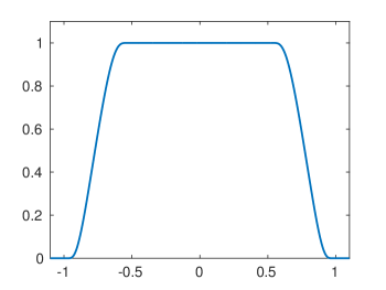
Figure 2: Windowing function $W$ for $c=0.5$.

As shown in [5] the smooth-windowing methodology converges super-algebraically fast away from Wood anomalies as $A\to\infty$, and thus this approach improves upon the shifted Green function convergence—at least away from Wood frequencies. Reference [5] establishes super-algebraic convergence to the corresponding quasi-periodic Green function in the context of the problem of scattering by bi-periodic structures in three-dimensional space. Similar ideas can be applied in the two-dimensional problem under consideration. In fact the proof is simpler in the present case—which does not require summation of doubly-infinite sums.

We can now consider the problem of evaluation of the operator $A_{k}$, whose inverse appears on the right-hand side of (53). Clearly, using (39) and the values of a given continuous function $\psi$ on the Nyström mesh, we can obtain the numerical values of $A_{k}\psi$ on the same Nyström mesh by numerical integration of the integral terms containing the Green function as well as those associated with the functionals $I^{+}_{n,k}$, followed by summation of the infinite sum over $n\not\in\mathcal{N}_{\mathrm{wa}}$ (whose general term decays exponentially, in accordance with (44)). Clearly, such an algorithm can be implemented in terms of a matrix-vector product for the vector which contains the discrete values of the function $\psi$. The inverse of the corresponding matrix provides the necessary discrete approximation of the operator $A_{k}^{-1}$. (In practice the action of the numerical inverse on a given vector can be obtained either by means of an iterative linear-algebra solver or, as in the approach followed in the present two-dimensional context, directly by means of Gaussian elimination.)

In order to complete the evaluation of the solution $\psi_{k}$ in (53) it is necessary to produce the the coefficients $d_{j}(k)$. But these values can be obtained by solving the $r\times r$ linear system (51) (cf. Remark 2). The necessary elements in this matrix equation can be produced as follows: the diagonal matrix $\mathcal{D}_{\boldsymbol{\beta}(k)}$ results from simple algebra, and the matrix $\mathcal{T}$ (equation (50)) and right-hand side $c(k)$ (right below equation (49)) can be produced through respective applications of the aforementioned matrix form of the operator $A_{k}^{-1}$ followed by numerical integration and simple algebra.

The case in which $k$ is away from Wood anomalies, finally, can be treated by means of a slightly modified version of the “Wood and near-Wood” strategy described above—since, as it is readily checked, the operator $A_{k}$ in equation (39) and the mixed integral/Rayleigh-series operator in equation (31) differ only by the finite sum of terms with $n\in\mathcal{N}_{\mathrm{wa}}$. Thus, for a configuration away from Wood anomalies it is only necessary to incorporate those terms which were excluded to obtain $A_{k}$ in the near Wood-anomaly case. (Note, however, that, away from Wood frequencies on may select $j=0$ in (31), in which case the sum on the left-hand side of this equation vanishes, and a classical formulation is recovered.) In any case, the resulting discrete formulations can be inverted by means of an iterative solver or, for sufficiently small discretizations, by means of Gaussian elimination.

6 Numerical results

This section presents numerical tests and examples that demonstrate the character of the scattering solvers introduced in the previous section, with an emphasis on the impact of the Wood-anomaly methods described in Section 4.3. Detailed numerical results presented in what follows concern, in particular, the invertibility of the operator $A_{k}$ around Wood frequencies (see Theorem 2 and discussion immediately thereafter), as well as the conditioning, accuracy and computing costs associated with the proposed methodology for ranges of frequencies which, once again, include Wood anomalies. All solutions presented in this section were produced by means of a Fortran implementation of the algorithms described in Section 5, together with the LAPACK Gaussian elimination routines, on a single core of an Intel i7-4600M processor.

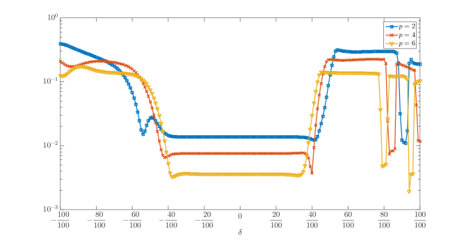
Figure 3: Smallest singular values of the discrete approximation $\tilde{A}_{k}$ of the operator $A_{k}$, for the scattering structure described in the text, as a function of $\delta$ ($k=k_{0}+\delta^{8}$), around the Wood frequencies $k_{0}=p\frac{2\pi}{L(1+\sin(\theta))}$ with $p=2,4,6$. (For reference, the maximum condition numbers $\kappa=\sigma_{\mathrm{max}}/\sigma_{\mathrm{min}}$ for the cases $p=2$, $4$ and $6$ are approximately $280$, $1508$ and $2401$, respectively.) Note that, in particular, the smallest singular values for $\delta^{8}=10^{-16}$ and $\delta=0$ ($k_{0}\in\mathcal{K}_{\mathrm{wa}}$) are included in this graph.

6.1 Invertibility and conditioning at and around Wood frequencies

In order to provide numerical evidence of the invertibility of the operator $A_{k}$ (equation (39)) for $k$ in a neighborhood of $k_{0}\in\mathcal{K}_{\mathrm{wa}}$ we consider the maximum and minimum singular values for a discretization of the operator $A_{k}$ based on $n_{i}=64$ Nyström nodes (see Section 5), with varying values of both, the window-size parameter $A$ and the number $j$ of shifts, and with $N_{ev}=20$ (see Section 5). We have found that, in all cases the maximum singular values of $A_{k}$ do not grow as $k$ approaches $k_{0}$, and that the minimum singular values are all bounded away from zero. For definiteness we present examples for the fairly generic test geometry depicted in Figure 1 with $L=4$ and $\theta=0$; similar results were obtained for periodic arrays of cylinders of various cross sections and for other numbers $n_{i}$ of discretization points.

Figure 3 displays the smallest singular values of the discrete approximation $\tilde{A}_{k}$ of the operator $A_{k}$ in equation (39) obtained using $A=1600\cdot L$ together with a $64$-point discretization of the scatterer $D_{0}$ depicted in Figure 1. In order to provide close refinements near several Wood anomalies we use the parameters $\delta$ defined by $k=k_{0}+\mathrm{sign}(\delta)\cdot\delta^{8}$ for $k_{0}=p\frac{2\pi}{L(1+\sin(\theta))}\in\mathcal{K}_{\mathrm{wa}}$ with $p=2,4,6$. (The $\delta$ parametrization of the frequency domain is used to achieve a fine resolution near the Wood anomaly values corresponding to $\delta=0$ for each one of the integers $p=2,4,6$.) Visually indistinguishable curves for both smallest and largest singular values are obtained using a 128-point discretization of $D_{0}$ (while fixing the value $A=1600L$), which suggests that the approximate singular values provide close approximations of the corresponding smallest and largest singular values of the continuous operator $A_{k}$. Clearly, the smallest singular value $\sigma_{\mathrm{min}}$ remains bounded in the limit as $\delta\to 0$.

Figure 4 presents the energy balance errors (given by the the left-hand side of equation (10) for efficiencies values $e^{\pm}_{n}$ computed numerically with $n_{i}=64$) as a function of $\delta$, with window-size $A=LN_{per}$ and for two values of the shift-parameter $j$ (equations (18) and (20)); a shifted Green function with a number $j=5$ of shifts and spacing $h=3.5$ was used in all cases. Studies based on use of finer integration meshes and larger window sizes suggest that the actual solution errors are well described by the energy-balance curves presented in this figure. This figure demonstrates clearly the beneficial effect induced by the presence of the Green-function shifts.

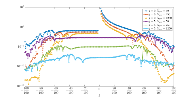
Figure 4: Energy balance error, as a function of $\delta$ ($k=k_{0}+\delta^{8}$ with $k_{0}=\frac{2\pi}{L(1+\sin(\theta))}$), resulting from use of the methodology introduced in Section 4.3 with $j=0$ (un-shifted Windowed Green function) and $j=5$ (five-shift Windowed Green function) for a configuration with $L=4$ and $\theta=0$ (normal incidence). The beneficial effect induced by the use of the shifted Green-function and Sherman-Morrison inversion (cf. Theorem 2) can be clearly appreciated.

6.2 Computing cost

The Green-function representations and solvers presented in this paper give rise to fast numerical algorithms: like the rough-surface solvers [7], the present methods for periodic arrays of scatterers enable evaluation of highly-accurate scattering solutions, with frequencies away, at and around Wood anomalies, in computing times of the order of hundreds of milliseconds. In particular, the approach is highly competitive with other available solvers even for configurations away from Wood anomalies [2, 8]. The method can be additionally accelerated by means of FFT-based approaches [10, 5]; use of such acceleration methods in conjunction with shifted Green functions will be described elsewhere.

Sections 6.2.1, 6.2.2 and 6.2.3 present computing times required by the present solver for problems of scattering by periodic arrays (period $L=2\pi$) of circular cylinders. Examples for arrays of cylinders of radii $R=0.05L$, $R=0.1L$ and $R=0.25L$, and configurations far from Wood anomalies, at Wood anomalies and around Wood anomalies are considered. Incidence angles in Littrow mount of order $\ell=-1$ (for which the scattered plane-wave of order $\ell=-1$ propagates in the backscattering direction) were used; such a configuration is obtained provided the triplet $(k,L,\theta)$ verifies the relation $kL\sin(\theta)=\pi$. As noted in the previous section, Wood frequencies can be obtained by enforcing the relation $k_{0}=\frac{2\pi}{L(1+\sin(\theta))}n$ for some positive integer $n$; it can be easily checked that under the Littrow-mount assumption, the Wood-frequency condition reduces to $k_{0}L=(2n-1)\pi$ for some positive integer $n$. In what follows we consider the particular case $n=2$, which yields the Wood frequency $k_{0}=1.5\cdot\frac{2\pi}{L}$ (for which $\mathcal{N}_{\mathrm{wa}}=\{1,-2\}$; see Remark 2). In particular, $k=1\cdot\frac{2\pi}{L}$ is not a Wood frequency while the frequency $k=1.49\cdot\frac{2\pi}{L}$ is close to the Wood frequency $k_{0}$.

Throughout this section the computing times cited sufficed to produce full scattering solutions with an energy balance error of the order of $10^{-8}$.

6.2.1 Computing cost I: wave-numbers away from Wood anomalies

Tables 1, 2 and 3 present the computing times required by the proposed algorithm to evaluate the scattered field with an energy-balance error of the order of $10^{-8}$ for the wavenumber $k=1\cdot L$ (away from Wood anomalies).

Table 1: Cylinders of radius $R=0.05L$ at the frequency $k=1\cdot\frac{2\pi}{L}$.

$j$	0	1	2	3	4
$n_{i}$	18	16	18	18	18
$N_{per}$	100	30	45	24	22
$N_{ev}$	0	18	18	16	16
Time (s)	0.06	0.04	0.08	0.08	0.07

Table 2: Cylinders of radius $R=0.1L$ at the frequency $k=1\cdot\frac{2\pi}{L}$.

$j$	0	1	2	3	4
$n_{i}$	18	16	16	16	18
$N_{per}$	125	38	38	37	36
$N_{ev}$	0	20	20	20	20
Time (s)	0.1	0.07	0.07	0.08	0.09

Table 3: Cylinders of radius $R=0.25L$ at the frequency $k=1\cdot\frac{2\pi}{L}$.

$j$	0	1	2	3	4
$n_{i}$	20	14	14	14	16
$N_{per}$	125	66	75	73	58
$N_{ev}$	0	10	10	10	10
Time (s)	0.13	0.06	0.09	0.11	0.13

6.2.2 Computing cost II: a Wood anomaly frequency

Tables 6, 5 and 6 present results for the structures considered in the previous section except for the frequency, which is here taken to equal the Wood frequency $k=1.5\cdot L$. The best computing costs are now $0.14$, $0.6$ and $2.6$ seconds. These times are thus somewhat higher than the corresponding $0.04$, $0.07$ and $0.06$ times required for the non-Wood frequency $k=1\cdot L$.

Table 4: Cylinders of radius $R=0.05L$ at the Wood frequency $k=1.5\cdot\frac{2\pi}{L}$.

$j$	1	2	3	4	5	6
$n_{i}$	18	20	16	18	18	18
$N_{per}$	450	600	100	100	50	30
$N_{ev}$	20	20	20	20	20	20
Time (s)	0.62	0.8	0.25	0.31	0.19	0.14

Table 5: Cylinders of radius $R=0.1L$ at the Wood frequency $k=1.5\cdot\frac{2\pi}{L}$.

$j$	1	2	3	4	5	6
$n_{i}$	18	18	16	18	18	18
$N_{per}$	3500	5500	500	400	200	200
$N_{ev}$	20	20	20	20	20	20
Time (s)	2.35	3.96	0.7	0.6	0.7	0.8

Table 6: Cylinders of radius $R=0.25L$ at the Wood frequency $k=1.5\cdot\frac{2\pi}{L}$.

$j$	1	2	3	4	5	6
$n_{i}$	20	20	20	20	20	20
$N_{per}$	38500	42000	2500	2000	1000	750
$N_{ev}$	20	20	20	20	20	20
Time (s)	32.1	35.5	4.5	4.5	2.6	2.6

6.2.3 Computing cost III: frequencies near Wood anomalies

Tables 7, 8 and 9 present results for the structures considered in the previous two sections, but now for the near-Wood frequency $k=1.49\cdot L$. The computing times are comparable to Wood-frequency times presented in the previous section.

Table 7: Cylinders of radius $R=0.05L$ at the frequency $k=1.49\frac{2\pi}{L}$.

$j$	0	1	2	3	4	5	6
$n_{i}$	18	16	16	16	16	18	18
$N_{per}$	3700	850	650	200	200	100	75
$N_{ev}$	0	20	20	20	20	20	20
Time (s)	3.2	0.59	0.5	0.36	0.4	0.37	0.32

Table 8: Cylinders of radius $R=0.1L$ at the frequency $k=1.49\frac{2\pi}{L}$.

$j$	0	1	2	3	4	5	6
$n_{i}$	18	18	18	18	18	18	18
$N_{per}$	3700	900	1000	350	320	175	100
$N_{ev}$	0	20	20	20	20	20	20
Time (s)	3.2	0.76	0.91	0.46	0.49	0.47	0.4

Table 9: Cylinders of radius $R=0.25L$ at the frequency $k=1.49\frac{2\pi}{L}$.

$j$	0	1	2	3	4	5	6
$n_{i}$	20	20	20	20	20	20	20
$N_{per}$	3700	1200	1000	600	600	400	380
$N_{ev}$	0	10	10	20	20	20	20
Time (s)	3.2	1.21	1.14	1.05	0.99	1.07	1.56

7 Conclusions

This paper introduced a new methodology for solutions of problems of scattering by periodic arrays of cylinders with applicability throughout the spectrum—even at and around Wood frequencies. To the best of our knowledge, this is the first particle-array periodic-Green-function method that remains applicable around Wood frequencies. The algorithm yields fast solutions for frequencies in the resonance region, where wavelengths are comparable to the structural period. High-frequency problems are also amenable to efficient treatment by these methods in conjunction FFT-based acceleration approaches [10, 5]; the development of such accelerated methods, however, is left for future work.

Appendix A Rayleigh expansion of $v_{k_{0}}$ for $k_{0}\in\mathcal{K}_{\mathrm{wa}}$

The Rayleigh expansion of $v_{k_{0}}$ can be obtained by substituting the Rayleigh series of the shifted Green function $G_{j,k_{0}}^{q}$ for $k_{0}\in\mathcal{K}_{\mathrm{wa}}$ in equation (47). In the case $j\geq 2$ we have [7, eqs. (54), (56)]

$$G_{j,k_{0}}^{q}(X,Y)=\frac{i}{2L}\sum\limits_{n\not\in\mathcal{N}_{\mathrm{wa}}}\frac{(1-e^{i\beta_{n}(k_{0})})^{j}}{\beta_{n}(k_{0})}e^{i\alpha_{n}(k)X+i\beta_{n}(k)Y}$$ (66)

for $Y>0$, while, for $-h<Y<0$, the corresponding modified version of equation [7, eq. (54)] yields

$$G_{j,k_{0}}^{q}(X,Y)=\frac{i}{2L}\sum\limits_{n\not\in\mathcal{N}_{\mathrm{wa}}}\frac{e^{i\alpha_{n}(k)X-i\beta_{n}(k)Y}}{\beta_{n}(k_{0})}+\frac{(1-e^{i\beta_{n}(k_{0})})^{j}-1}{\beta_{n}(k_{0})}e^{i\alpha_{n}(k)X+i\beta_{n}(k)Y}+\frac{1}{L}\sum\limits_{n\in\mathcal{N}_{\mathrm{wa}}}Ye^{i\alpha_{n}(k_{0})X}.$$ (67)

The analogous expressions for $j=1$ are

$$G_{j,k_{0}}^{q}(X,Y)=\frac{i}{2L}\sum\limits_{n\not\in\mathcal{N}_{\mathrm{wa}}}\frac{(1-e^{i\beta_{n}(k_{0})})^{j}}{\beta_{n}(k_{0})}e^{i\alpha_{n}(k)X+i\beta_{n}(k)Y}+\frac{h}{2L}\sum\limits_{n\in\mathcal{N}_{\mathrm{wa}}}e^{i\alpha_{n}(k_{0})X}$$ (68)

for $Y>0$ and

$$G_{j,k_{0}}^{q}(X,Y)=\frac{i}{2L}\sum\limits_{n\not\in\mathcal{N}_{\mathrm{wa}}}\frac{e^{i\alpha_{n}(k)X-i\beta_{n}(k)Y}}{\beta_{n}(k_{0})}+\frac{(1-e^{i\beta_{n}(k_{0})})^{j}-1}{\beta_{n}(k_{0})}e^{i\alpha_{n}(k)X+i\beta_{n}(k)Y}+\frac{1}{L}\sum\limits_{n\in\mathcal{N}_{\mathrm{wa}}}(\frac{h}{2}+Y)e^{i\alpha_{n}(k_{0})X}$$ (69)

for $-h<Y<0$. For $j\geq 2$ we thus obtain

$$v_{k_{0}}(x,y)=\frac{i}{2L}\sum\limits_{n\not\in\mathcal{N}_{\mathrm{wa}}}\frac{I_{n,k_{0}}^{+}[\psi]}{\beta_{n}(k)}e^{i\alpha_{n}(k)x+i\beta_{n}(k)y}$$ (70)

in the region $\{y>M^{+}\}$ and

$$v_{k_{0}}(x,y)=\frac{i}{2L}\sum\limits_{n\not\in\mathcal{N}_{\mathrm{wa}}}\frac{I_{n,k_{0}}^{-}[\psi]}{\beta_{n}(k_{0})}e^{i\alpha_{n}(k_{0})x-i\beta_{n}(k_{0})y}+\frac{1}{L}\sum\limits_{n\in\mathcal{N}_{\mathrm{wa}}}I_{n,k_{0}}^{+}[\psi]ye^{i\alpha_{n}(k_{0})x}-\tilde{I}_{n,k_{0}}[\psi]e^{i\alpha_{n}(k_{0})x}$$ (71)

in the region $\{y<M^{-}\}$ (see Figure 1). Here, the functional $\tilde{I}_{n,k_{0}}$ is defined in equation (59); note, further, that for $n\in\mathcal{N}_{\mathrm{wa}}$ we have $I^{+}_{n,k_{0}}=I^{-}_{n,k_{0}}$.

In the case $j=1$, finally, we obtain

$$v_{k_{0}}(x,y)=\frac{i}{2L}\sum\limits_{n\not\in\mathcal{N}_{\mathrm{wa}}}\frac{I_{n,k_{0}}^{+}[\psi]}{\beta_{n}(k)}e^{i\alpha_{n}(k)x+i\beta_{n}(k)y}+\frac{h}{2L}\sum\limits_{n\in\mathcal{N}_{\mathrm{wa}}}I^{+}_{n,k_{0}}[\psi]e^{i\alpha_{n}(k_{0})x}$$ (72)

in the region $\{y>M^{+}\}$ and

$$v_{k_{0}}(x,y)=\frac{i}{2L}\sum\limits_{n\not\in\mathcal{N}_{\mathrm{wa}}}\frac{I_{n,k_{0}}^{-}[\psi]}{\beta_{n}(k_{0})}e^{i\alpha_{n}(k_{0})x-i\beta_{n}(k_{0})y}+\frac{1}{L}\sum\limits_{n\in\mathcal{N}_{\mathrm{wa}}}I_{n,k_{0}}^{+}[\psi]ye^{i\alpha_{n}(k_{0})x}+\left(\frac{h}{2}I_{n,k_{0}}^{+}[\psi]-\tilde{I}_{n,k_{0}}[\psi]\right)e^{i\alpha_{n}(k_{0})x}$$ (73)

in the region $\{y<M^{-}\}$ (see Figure 1).

Remark 4.

From equations (71) and (73) we see that that the potential $v_{k_{0}}$ could in principle contain unbounded modes (that grow linearly with $y$) in the region $\{y<M^{-}\}$—and, thus, the solution $v_{k_{0}}$ could in principle fail to satisfy the radiation condition put forth in Remark 1. The unbounded modes are not present in the expansions (71) and (73) provided the density $\psi$ satisfies the conditions $I_{n,k_{0}}^{+}[\psi]=0$ for all $n\in\mathcal{N}_{\mathrm{wa}}$. But, in view of equation (51) and the parenthetical comment that follows (52), equation (57) tells us that $I_{n_{j},k}^{+}$ ($j=1,\dots,r$) vanishes for $k=k_{0}$—since so does the denominator on the left hand side of that equation. Since $n_{j}$ ($j=1,\dots,r$) is an enumeration of $\mathcal{N}_{\mathrm{wa}}$ we see that the density $\psi_{k_{0}}$ obtained at a Wood anomaly in Theorem 2 indeed satisfies the condition $I_{n,k_{0}}^{+}[\psi]=0$ for all $n\in\mathcal{N}_{\mathrm{wa}}$. It follows that the corresponding potential $v_{k_{0}}$ (defined in terms of $\psi_{k_{0}}$) is a radiating potential both above and below the obstacles.

Remark 5.

In connection with the previous remark we note that the functionals $I_{n,k_{0}}^{+}[\psi]$ ($n\in\mathcal{N}_{\mathrm{wa}}$) do not identically vanish: e.g., setting $\psi=e^{i\alpha_{n}x}$ in (30) yields a non-zero value, since the integral involving the normal derivative does vanish. It follows that, for a given (arbitrary) density $\psi$, the potential $v_{k_{0}}$ does not generally satisfy the radiation condition and, therefore, as indicated in Section 4.3, classical arguments based on uniqueness of radiating solution for the associated PDE problem are not immediately applicable to the study of uniqueness of the operator $A_{k_{0}}$ with $k_{0}\in\mathcal{K}_{\mathrm{wa}}$.

Appendix B Invertibility of $\tilde{R}_{k_{0}}A_{k_{0}}^{-1}$

Using the representations (70) and (71) (in the case $j\geq 2$) or (72) and (73) (in the case $j=1$) we can now deduce the invertibility of the restriction of the operator $\tilde{R}_{k_{0}}A_{k_{0}}^{-1}$ to the finite-dimensional space $S$ (see Theorem 2) provided uniqueness of solution of the problem (2)–(3) holds for $k=k_{0}$. Indeed, for $f\in S$ such that $\tilde{R}_{k_{0}}A_{k_{0}}^{-1}f=0$, in view of equation (37) we must have $I_{n,k_{0}}^{+}[A_{k_{0}}^{-1}f]=0$ for all $n\in\mathcal{N}_{\mathrm{wa}}$. In view of Remark 4, then, the potential $v_{k_{0}}$ defined in (47) with $\psi=A_{k_{0}}^{-1}f$ is a radiating solution of the Helmholtz equation. Moreover, using the jump-relations of the single and double layer potentials it follows that $v_{k_{0}}$ equals $f$ along the boundary of $D_{0}$. But, since $f\in S$,

$$f=\sum\limits_{n\in\mathcal{N}_{\mathrm{wa}}}C_{n}e^{i\alpha_{n}(k)x},$$ (74)

it follows (assuming the uniqueness of radiating solutions for the PDE problem for $k=k_{0}$) that

$$v_{k}(x,y)=\sum\limits_{n\in\mathcal{N}_{\mathrm{wa}}}C_{n}e^{i\alpha_{n}(k)x}$$ (75)

in the complete exterior domain $\Omega=\mathbb{R}^{2}\setminus D$. Since $I_{n,k_{0}}^{+}[\psi]=0$, $n\in\mathcal{N}_{\mathrm{wa}}$ then $v_{k}$ does not contain the Wood modes in the region $y>M^{+}$ (see equations (70) or (72) in the respective cases $j\geq 2$ and $j=1$) and therefore $C_{n}=0$ for all $n\in\mathcal{N}_{\mathrm{wa}}$. In other words, the operator $\tilde{R}_{k_{0}}A_{k_{0}}^{-1}:S\to S$ in finite-dimensional vector space $S$ has trivial null space, and it must therefore be invertible, as desired.

References

- [1] Tilo Arens, Kai Sandfort, Susanne Schmitt, and Armin Lechleiter. Analysing Ewald’s method for the evaluation of Green’s functions for periodic media. IMA Journal of Applied Mathematics, 78(3):405–431, 2013.
- [2] Alex Barnett and Leslie Greengard. A New integral Representation for Quasi-periodic Fields and Its Application to Two-dimensional Band Structure Calculations. J. Comput. Phys., 229(19):6898–6914, September 2010.
- [3] Alex Barnett and Leslie Greengard. A new integral representation for quasi-periodic scattering problems in two dimensions. BIT Numerical Mathematics, 51(1):67–90, 2011.
- [4] Helmut Brakhage and Peter Werner. Über das Dirichletsche Außenraumproblem für die Helmholtzsche Schwingungsgleichung. Archiv der Mathematik, 16(1):325–329, 1965.
- [5] O. P. Bruno, S. P. Shipman, C. Turc, and S. Venakides. Efficient Evaluation of Doubly Periodic Green Functions in 3d Scattering, Including Wood Anomaly Frequencies. Available at https://arxiv.org/abs/1307.1176v1, July 2013.
- [6] Oscar Bruno, Tim Elling, and Catalin Turc. Regularized integral equations and fast high-order solvers for sound-hard acoustic scattering problems. International Journal for Numerical Methods in Engineering, 91(10):1045–1072, 2012.
- [7] Oscar P. Bruno and Bérangère Delourme. Rapidly convergent two-dimensional quasi-periodic Green function throughout the spectrum - including Wood anomalies. J. Comput. Physics, 262:262–290, 2014.
- [8] Oscar P. Bruno and Michael C. Haslam. Efficient high-order evaluation of scattering by periodic surfaces: deep gratings, high frequencies, and glancing incidences. J. Opt. Soc. Am. A, 26(3):658–668, Mar 2009.
- [9] Oscar P. Bruno and Michael C. Haslam. Efficient high-order evaluation of scattering by periodic surfaces: vector-parametric gratings and geometric singularities. Waves in Random and Complex Media, 20(4):530–550, 2010.
- [10] Oscar P Bruno and Leonid A Kunyansky. A fast, high-order algorithm for the solution of surface scattering problems: basic implementation, tests, and applications. Journal of Computational Physics, 169(1):80–110, 2001.
- [11] Oscar P. Bruno and Fernando Reitich. Solution of a boundary value problem for the Helmholtz equation via variation of the boundary into the complex domain. Proceedings of the Royal Society of Edinburgh: Section A Mathematics, 122:317–340, 1 1992.
- [12] F. Capolino, D.R. Wilton, and W.A. Johnson. Efficient computation of the 3d Green’s function for the Helmholtz operator for a linear array of point sources using the Ewald method. Journal of Computational Physics, 223(1):250 – 261, 2007.
- [13] S.N. Chandler-Wilde and D.C. Hothersall. Efficient calculation of the green function for acoustic propagation above a homogeneous impedance plane. Journal of Sound and Vibration, 180(5):705 – 724, 1995.
- [14] Andrew Dienstfrey, Fengbo Hang, and Jingfang Huang. Lattice sums and the two-dimensional, periodic Green’s function for the Helmholtz equation. Proceedings of the Royal Society of London A: Mathematical, Physical and Engineering Sciences, 457(2005):67–85, 2001.
- [15] R. Kress. Linear integral equations. Springer-Verlag, 1999.
- [16] Harun Kurkcu and Fernando Reitich. Stable and efficient evaluation of periodized Green’s functions for the Helmholtz equation at high frequencies. Journal of Computational Physics, 228(1):75–95, 2009.
- [17] R. Kussmaul. Ein numerisches Verfahren zur Lösung des Neumannschen Ausssenraumproblems für die Helmholtzsche Schwingungsgleichung. Computing, 4(3):246–273, 1969.
- [18] Rolf Leis. Zur Dirichletschen Randwertaufgabe des Aussenraumes der Schwingungsgleichung. Mathematische Zeitschrift, 90(3):205–211, 1965.
- [19] C. M. Linton. Lattice sums for the Helmholtz equation. SIAM Review, page 2010.
- [20] C.M. Linton. The Green’s Function for the Two-Dimensional Helmholtz Equation in Periodic Domains. Journal of Engineering Mathematics, 33(4):377–401, 1998.
- [21] Erich Martensen. Über eine Methode zum räumlichen Neumannschen Problem mit einer Anwendung für torusartige Berandungen. Acta Mathematica, 109(1):75–135, 1963.
- [22] Andrew W Mathis and Andrew F Peterson. A comparison of acceleration procedures for the two-dimensional periodic Green’s function. Antennas and Propagation, IEEE Transactions on, 44(4):567–571, 1996.
- [23] John A. Monro. A super-algebraically convergent, Windowing-based approach to the evaluation of scattering from periodic rough surfaces. PhD thesis, 2007.
- [24] Alexander Moroz. Exponentially convergent lattice sums. Optics letters, 26(15):1119–1121, 2001.
- [25] NA Nicorovici and RC McPhedran. Lattice sums for off-axis electromagnetic scattering by gratings. Physical Review E, 50(4):3143, 1994.
- [26] NA Nicorovici, RC McPhedran, and R Petit. Efficient calculation of the green’s function for electromagnetic scattering by gratings. Physical Review E, 49(5):4563, 1994.
- [27] O.I. Panich. On the question of the solvability of the exterior boundary-value problems for the wave equation and Maxwell’s equations. Russian Math. Surveys, 20:221–226, 1965.
- [28] R. Petit. Electromagnetic theory of gratings. Springer-Verlag, 1980.
- [29] William H Press. FORTRAN Numerical Recipes: Numerical recipes in FORTRAN 90. Cambridge University Press, 1996.
- [30] Lord Rayleigh O.M. P.R.S. Note on the remarkable case of diffraction spectra described by Prof. Wood. Philosophical Magazine Series 6, 14(79):60–65, 1907.
- [31] D. Colton R. Kress. Integral equation methods in Scattering theory. Wiley and Sons, 1983.
- [32] D. Colton R. Kress. Inverse acoustic and electromagnetic Scattering Theory. Springer-Verlag New York, 2013.
- [33] R W Wood. On a Remarkable Case of Uneven Distribution of Light in a Diffraction Grating Spectrum. Proceedings of the Physical Society of London, 18(1):269, 1902.