On the probability of positive-definiteness in the gGUE via semi-classical Laguerre polynomials

Abstract

In this paper, we compute the probability that an $N\times N$ matrix from the generalised Gaussian Unitary Ensemble (gGUE) is positive definite, extending a previous result of Dean and Majumdar [17]. For this purpose, we work out the large degree asymptotics of semi-classical Laguerre polynomials and their recurrence coefficients, using the steepest descent analysis of the corresponding Riemann–Hilbert problem.

1 Introduction and main results

The Gaussian Unitary Ensemble (GUE) is the most classical and studied example of a unitarily invariant Hermitian random matrix ensemble. Given the set of $N\times N$ Hermitian matrices $\mathcal{H}_{N}$, one defines a probability measure

$$dP(M_{N})=\frac{1}{\mathcal{Z}_{N}}e^{-N\,\mathrm{Tr}V(M_{N})}dM_{N},$$ (1.1)

where $dM_{N}$ is the Lebesgue measure on the independent entries of $M_{N}$, and $\mathcal{Z}_{N}$ is the partition function:

$$\mathcal{Z}_{N}=\int_{\mathcal{H}_{N}}e^{-N\,\mathrm{Tr}V(M_{N})}dM_{N}.$$ (1.2)

The potential $V$ is a smooth function with sufficient growth at infinity, so that (1.2) is well defined, and the GUE corresponds to the quadratic case $V(x)=x^{2}$, see references [3, 25, 30] for relevant background.

In this paper we are interested in the probability that matrices drawn at random from (1.1) are positive definite, denoted here by $\mathbb{P}(M_{N}>0)$. As well as being a natural question within random matrix theory, in several situations in the physics literature $M_{N}$ is used to model the Hessian matrix of random high-dimensional energy surfaces, see e.g. [1, 12, 17, 26] and references therein. In such contexts $\mathbb{P}(M_{N}>0)$ provides important information on the stability (maxima and minima) of such energy surfaces. Outside physics, this question turns out to appear explicitly in certain number theoretical problems [5].

In the GUE case, the earliest investigations of this probability appeared in the string theory and cosmology literature [1], where it was argued that $\mathbb{P}(M_{N}>0)$ decays exponentially in $N^{2}$ (at least implicitly, this already followed from the large deviations principle of Ben Arous and Guionnet [4]). However, the multiplicative constant in these asymptotics remained unknown until the work of Dean and Majumdar [17], who showed using Coulomb gas techniques that

$$\log\mathbb{P}(M_{N}>0)=-c_{1}N^{2}+o(N^{2})$$ (1.3)

where

$$c_{1}=\frac{\log 3}{2}.$$ (1.4)

Then in subsequent work [10], further terms in the asymptotic expansion of (1.3) were computed using the technique of loop equations, where it was shown that

$$\log\mathbb{P}(M_{N}>0)=-c_{1}N^{2}+c_{2}\log(N)+c_{3}+o(1)$$ (1.5)

where

$$c_{2}=-\frac{1}{12},\qquad c_{3}=\frac{\log 3}{8}-\frac{\log 2}{6}+\zeta^{\prime}(-1),$$ (1.6)

and $\zeta(s)$ is the Riemann zeta function. Under certain technical assumptions, Borot and Guionnet [8] later developed a rigorous mathematical basis for the application of the loop equations, so that (1.5) can be said to constitute a rigorously established result. Our aim will be to give a simple, unified proof of (1.5) using the methods of orthogonal polynomials. Our results also apply to the generalised GUE, leading to a 1-parameter extension of the asymptotics (1.5), which as far as we are aware have not appeared in either the mathematics or physics literature.

Like the ordinary GUE, the generalised GUE is defined on the set of $N\times N$ Hermitian matrices, but now the probability measure has the form

$$dP(M_{N})=\frac{|\det(M_{N})|^{\lambda}}{\mathcal{Z}^{\mathrm{gGUE}}_{N}}\,\mathrm{exp}\left(-N\,\mathrm{Tr}(M_{N}^{2})\right)dM_{N},$$ (1.7)

where we assume $\lambda>-1$ to ensure finiteness of the normalizing constant $\mathcal{Z}^{\mathrm{gGUE}}_{N}$:

$$\mathcal{Z}^{\mathrm{gGUE}}_{N}=\int_{\mathcal{H}_{N}}|\det(M_{N})|^{\lambda}\,\mathrm{exp}\left(-N\,\mathrm{Tr}(M_{N}^{2})\right)dM_{N}.$$ (1.8)

This partition function depends implicitly on $\lambda$, although for simplicity of notation we do not emphasize it. Ensembles of the form (1.7), with extra algebraic terms in the density, were studied extensively in the literature on matrix models under the name Gauss-Penner model, see [20, 2] for details and applications.

The main purpose of this paper is to prove the following

Theorem 1.1.

Let $\mathbb{P}(M^{(\lambda)}_{N}>0)$ denote the probability that a random matrix from ensemble (1.7) is positive definite. Then for any fixed $\lambda>-1$, we have the asymptotic expansion as $N\to\infty$,

$$\begin{split}&\log\mathbb{P}(M^{(\lambda)}_{N}>0)=-c_{1}N^{2}-\frac{\lambda\log(3)}{2}N+\left(c_{2}+\frac{\lambda^{2}}{4}\right)\log(N)+c_{3}\\ &+\frac{3\lambda^{2}}{4}\log(2)-\frac{\lambda^{2}}{2}\log(3)-\log\frac{G(\tfrac{3}{2})G(\tfrac{1}{2})G(\lambda+1)}{G(\tfrac{\lambda+3}{2})G(\tfrac{\lambda+1}{2})G(1)}+\mathcal{O}(N^{-1}),\end{split}$$ (1.9)

where $c_{1},c_{2}$ and $c_{3}$ are the explicit constants defined above and $G(z)$ is the Barnes G function [33, §5.17].

We note that in the case $\lambda=0$ we immediately recover the result (1.5) of [10] as a special case. We also mention the work [11] where the dependence of the leading term $c_{1}$ on growing $\lambda\sim N$ is investigated.

Figure 1 illustrates the accuracy of the asymptotic expansion (1.9) for increasing $N$ and several values of $\lambda$. The comparison has been made with respect to brute force calculation of the Hankel determinant expression for the partition functions, see Appendix A, which is quite time consuming and needs a large number of digits in Maple.

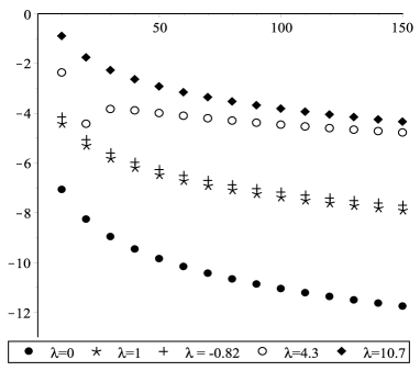
Figure 1: Absolute errors (in $\log_{10}$ scale) as a function of $N$ and for different values of $\lambda$, taking all the terms in (1.9) up to order $\mathcal{O}(1)$ (included).

To prove Theorem 1.1 we will study the partition function:

$$Z_{N}(s)=\int_{0}^{\infty}\ldots\int_{0}^{\infty}\prod_{j=1}^{N}w(x_{j};\lambda,s)\,\prod_{1\leq j<k\leq N}(x_{k}-x_{j})^{2}\,dx_{1}\ldots dx_{N}$$ (1.10)

where

$$w(x;\lambda,s)=x^{\lambda}e^{-N(x+s(x^{2}-x))}.$$ (1.11)

Note that this deformed weight interpolates between the classical Laguerre weight if $s=0$ and the generalized GUE if $s=1$. Diagonalizing $M_{N}$ in (1.7) and integrating out the eigenvectors (see e.g. [3, 25, 30]) we see that

$$\begin{split}\log\mathbb{P}(M^{(\lambda)}_{N}>0)&=\log\left(\frac{Z_{N}(1)}{Z_{N}^{\mathrm{gGUE}}}\right)\\ &=\int_{0}^{1}\frac{Z_{N}^{\prime}(s)}{Z_{N}(s)}\,ds+\log Z_{N}(0)-\log Z^{\mathrm{gGUE}}_{N}.\end{split}$$ (1.12)

As the quantities $Z_{N}(0)=Z^{\textrm{LUE}}_{N}$ and $Z_{N}^{\mathrm{gGUE}}$ turn out to have explicit evaluations in terms of Gamma functions (see Lemmas A.1 and A.2), our main task is to compute the integrand in (1.12).

1. We write $Z^{\prime}_{N}(s)/Z_{N}(s)$ in terms of the recurrence coefficients of a suitable family of semiclassical Laguerre polynomials, orthogonal with respect to $w(x;\lambda,s)$ on $x\in[0,\infty)$.

2. We compute the first terms in the asymptotic expansion of these recurrence coefficients as $N\to\infty$, using the corresponding Riemann–Hilbert problem and the Deift–Zhou method of steepest descent.

3. We show that such asymptotic expansions are uniform in $s\in[0,1]$ and we integrate term by term in (1.12).

2 Proof of Theorem 1.1

Semi-classical Laguerre orthogonal polynomials (OPs): $\pi_{n,N}(x)=\pi_{n,N}(x;\lambda,s)$ are defined by the orthogonality

$$\int_{0}^{\infty}\pi_{n,N}(x)x^{k}w(x;\lambda,s)dx=0,\qquad k=0,1,2,\ldots,n-1$$ (2.1)

and the normalization

$$\int_{0}^{\infty}\pi^{2}_{n,N}(x)w(x;\lambda,s)dx=h_{n,N}(\lambda,s)\neq 0,\qquad n\geq 0,$$ (2.2)

where we write the weight function (1.11) as

$$w(x;\lambda,s)=x^{\lambda}e^{-NV(x;s)},\qquad\lambda>-1$$ (2.3)

and $N>0$ is a real parameter. Here the potential is

$$V(x;s)=x+s(x^{2}-x),$$ (2.4)

constructed in such a way that $V(x;0)=V(x)=x$ corresponds to the classical Laguerre OPs, while $V(x;1)=x^{2}$ is the potential that we are interested in.

Remark 2.1.

The deformation (2.4) follows a similar idea as the construction by Bleher and Its in [9]. The quantities considered here were also recently investigated in the complementary regime of fixed $N$ and large parameters by Clarkson and Jordaan [14]. Part of this interest stems from the fact that the recurrence coefficients for semi-classical Laguerre polynomials, with weight $w(x;\lambda,t)=x^{\lambda}\exp(-x^{2}+tx)$, satisfy deformation equations (in $t$) that are closely related to the Painlevé IV differential equation [7, 22, 14]. Different aspects of this relationship were also studied in [21, 38].

Since the weight function (1.11) is positive and integrable on $[0,\infty)$ for $s\in[0,1]$, it follows from general theory [13, 27], that the orthogonal polynomials $\pi_{n,N}(x)$ exist uniquely for all $n\geq 0$ and $s\in[0,1]$, and they satisfy $\deg\pi_{n,N}=n$. Furthermore, they are solutions of a three term recurrence relation (written in monic form):

$$x\pi_{n,N}(x)=\pi_{n+1,N}(x)+\alpha_{n,N}\pi_{n,N}(x)+\beta_{n,N}\pi_{n-1,N}(x),$$ (2.5)

with initial data $\pi_{-1,N}(x)=0$, $\pi_{0,N}(x)=1$, and with recurrence coefficients $\alpha_{n,N}=\alpha_{n,N}(\lambda,s)$ and $\beta_{n,N}=\beta_{n,N}(\lambda,s)$.

Remark 2.2.

For brevity, in the sequel, we will write $\alpha_{n}$ and $\beta_{n}$ instead of $\alpha_{n,N}$ and $\beta_{n,N}$, if no confusion arises, and similarly $h_{n}$ instead of $h_{n,N}$ in (2.2). We will also use $\pi_{n}(x)$ instead of $\pi_{n,N}(x)$ for the $N$-dependent orthogonal polynomials and $w(x)$ instead of $w(x;\lambda,s)$ for the weight function (1.11).

Next, we write $Z^{\prime}_{N}(s)/Z_{N}(s)$, where the derivative is taken with respect to $s$, in terms of these recurrence coefficients.

Lemma 2.3.

We have the following deformation equation

$$\frac{Z^{\prime}_{N}(s)}{Z_{N}(s)}=\beta_{N}c_{N,\lambda}(s)-N^{2}\left[(1-3s)E_{N}+2sF_{N}\right],$$ (2.6)

where

$$c_{N,\lambda}(s) :=N^{2}(3-s)+\lambda N$$ (2.7)

$$E_{N} :=\beta_{N}(\alpha_{N}+\alpha_{N-1})$$ (2.8)

$$F_{N} :=\beta_{N}(\beta_{N+1}+\beta_{N}+\beta_{N-1}+\alpha_{N}^{2}+\alpha_{N}\alpha_{N-1}+\alpha_{N-1}^{2})$$ (2.9)

Proof.

Differentiating (1.10) shows that

$$\frac{Z^{\prime}_{N}(s)}{Z_{N}(s)}=-N\mathbb{E}_{V}\left[\sum_{j=1}^{N}(x_{j}^{2}-x_{j})\right]$$ (2.10)

where $\mathbb{E}_{V}$ denotes expectation with respect to the joint probability density function proportional to

$$\prod_{j=1}^{N}x_{j}^{\lambda}e^{-NV(x_{j},\lambda,s)}\prod_{1\leq j<k\leq N}(x_{k}-x_{j})^{2}$$ (2.11)

and $x_{j}\in[0,\infty)$, $j=1,\ldots,N$. The latter expectation can be written

$$-N\mathbb{E}_{V}\left[\sum_{j=1}^{N}(x_{j}^{2}-x_{j})\right]=-N\int_{0}^{\infty}(x^{2}-x)\rho_{N}(x)\,dx$$ (2.12)

where $\rho_{N}(x)$ is the so-called ‘one-point correlation function’ or ‘eigenvalue density’ corresponding to (2.11), see e.g. [3, 30] for definitions and basic properties of this quantity. The equality (2.12) appears frequently in random matrix theory, appropriate references include [34, Eqn. 1.1.20 and Eqn. 1.1.41], see also [39, Eqn. 1.8] where it was used for a similar purpose. In particular it is known that $\rho_{N}(x)$ can be computed explicitly by means of the Christoffel-Darboux formula:

$$\rho_{N}(x)=w(x)\,\frac{\pi_{N}^{\prime}(x)\pi_{N-1}(x)-\pi_{N}(x)\pi_{N-1}^{\prime}(x)}{h_{N-1}}$$ (2.13)

Inserting (2.13) into (2.12) yields four different contributions which can all be written in terms of the recurrence coefficients $\alpha_{N}$ and $\beta_{N}$. One term vanishes due to

$$\int_{0}^{\infty}x\pi_{N-1}^{\prime}(x)\pi_{N}(x)w(x)\,dx=0,$$ (2.14)

a consequence of orthogonality. So (2.12) can be decomposed as $I=I_{1}+I_{2}+I_{3}$, where

$$I_{1} :=\frac{N}{h_{N-1}}\int_{0}^{\infty}x^{2}\pi_{N-1}^{\prime}(x)\pi_{N}(x)w(x)\,dx$$ (2.15)

$$I_{2} :=-\frac{N}{h_{N-1}}\int_{0}^{\infty}x^{2}\pi_{N}^{\prime}(x)\pi_{N-1}(x)w(x)\,dx$$ (2.16)

$$I_{3} :=\frac{N}{h_{N-1}}\int_{0}^{\infty}x\pi_{N}^{\prime}(x)\pi_{N-1}(x)w(x)\,dx$$ (2.17)

First observe that $I_{1}=N(N-1)\beta_{N}$ (as a consequence of $h_{N}/h_{N-1}=\beta_{N}$). An exercise in integration by parts shows that

$$I_{2} =N(N+1+\lambda)\beta_{N}-N^{2}(1-s)E_{N}-2sN^{2}F_{N}$$ (2.18)

$$I_{3} =(1-s)N^{2}\beta_{N}+N^{2}2sE_{N}$$ (2.19)

where

$$E_{N} :=\frac{1}{h_{N-1}}\int_{0}^{\infty}\pi_{N}(x)\pi_{N-1}(x)x^{2}w(x)\,dx$$ (2.20)

$$F_{N} :=\frac{1}{h_{N-1}}\int_{0}^{\infty}\pi_{N}(x)\pi_{N-1}(x)x^{3}w(x)\,dx$$ (2.21)

Combining all these terms yields (2.6). Finally the identities (2.8) and (2.9) follow from the three term recurrence relation (2.5). ∎

The recurrence coefficients in Lemma 2.3 can be computed by solving the following coupled system of recurrence relations in the limit $N\to\infty$.

Proposition 2.4 (String equations).

Let $n/N=q$ and $s\in[0,1]$, then the recurrence coefficients $\alpha_{n}$ and $\beta_{n}$ in (2.5) (omitting $N$ for brevity) satisfy

$$2s(\beta_{n+1}+\beta_{n}+\alpha_{n}^{2})+(1-s)\alpha_{n} =2q+\frac{\lambda+1}{N},$$ (2.22)

$$\beta_{n}\left(2s\alpha_{n}+1-s\right)\left(2s\alpha_{n-1}+1-s\right) =(2s\beta_{n}-q)\left(2s\beta_{n}-q-\frac{\lambda}{N}\right),$$

with the values at $s=0$ corresponding to the (scaled with $N$) Laguerre polynomials:

$$\alpha_{n}(0)=2q+\frac{\lambda+1}{N},\qquad\beta_{n}(0)=q\left(q+\frac{\lambda}{N}\right).$$

Proof.

The string equations are known from [7, Theorem 1.1], [22] adapting the potential $V(x;s)=x^{2}-sx$ to the present one. ∎

We remark in passing that Boelen and Van Assche [7] have shown that (2.22) can be obtained from an asymmetric discrete Painlevé IV equation by a limiting process.

To solve this system of equations asymptotically as $N\to\infty$, we exploit the following fact, the proof of which is postponed to the next section.

Proposition 2.5.

Let $n/N=q$. For any $\lambda>-1$, the recurrence coefficients $\alpha_{n}$ and $\beta_{n}$ in (2.5) (omitting $N$ for brevity) have asymptotic expansions in inverse powers of $N$, as $N\to\infty$:

$$\alpha_{n} =\alpha_{n}(q,\lambda,s)\sim\sum_{k=0}^{\infty}f_{k}(q,\lambda,s)N^{-k},$$ (2.23)

$$\beta_{n} =\beta_{n}(q,\lambda,s)\sim\sum_{k=0}^{\infty}g_{k}(q,\lambda,s)N^{-k}.$$

The coefficients $f_{k}(q,\lambda,s)$ and $g_{k}(q,\lambda,s)$ are real analytic functions of $s\in[0,1]$, and these expansions hold uniformly for $s$ in this interval.

With these ingredients in hand, we can now prove Theorem 1.1. We insert the expansions (2.23) into the recurrence (2.22) and equate terms with equal powers of $N$. At leading order the solution consistent with the values at $s=0$ is

$$f_{0}=\frac{s-1+\Delta}{6s},\qquad g_{0}=\frac{(\Delta+s-1)\Delta}{72s^{2}},$$ (2.24)

where $\Delta=\Delta(q,s)=\sqrt{s^{2}+24qs-2s+1}$. Next, we have

$$f_{1}=\frac{\lambda+1}{\Delta},\qquad g_{1}=\frac{(\Delta+s-1)\lambda}{12\Delta s}.$$ (2.25)

Higher order corrections can be computed systematically in Maple, but become quite cumbersome. If we substitute the terms up to order $\mathcal{O}(N^{-2})$ (included), with $n=N$ (so $q=1$) into the right hand side of (2.6), we get

$$\frac{Z^{\prime}_{N}(s)}{Z_{N}(s)}=A(s)N^{2}+B(s)N+C(s)+\mathcal{O}(N^{-1}),\qquad N\to\infty,$$ (2.26)

where

$$A(s) =\frac{\Delta^{3}(s+1)+s^{4}+34s^{3}-216s^{2}-34s-1}{432s^{3}},$$ (2.27)

$$B(s) =\frac{\lambda(s^{2}-12s-1+(s+1)\Delta)}{24s^{2}},$$ (2.28)

$$C(s) =\frac{\lambda^{2}(s+1)[s^{2}+6s+1+(s-1)\Delta]}{4s(s^{2}-10s+1)\Delta}$$ (2.29)

$$-\frac{(s+1)^{3}\Delta+(s^{2}-1)(s^{2}+14s+1)}{12s(s^{2}-10s+1)\Delta^{2}},$$ (2.30)

Now integrating from $s=0$ to $s=1$, we get

$$\int_{0}^{1}\frac{Z^{\prime}_{N}(s)}{Z_{N}(s)}ds =N^{2}\int_{0}^{1}A(s)ds+N\int_{0}^{1}B(s)ds+\int_{0}^{1}C(s)ds+\mathcal{O}(N^{-1})$$ (2.31)

$$=N^{2}\left(\frac{3}{4}-\frac{\log 6}{2}\right)+N\left(\frac{1}{2}-\frac{\log 6}{2}\right)\lambda$$

$$+\frac{\lambda^{2}\log(2/3)}{2}+\frac{\log 3}{8}-\frac{\log 2}{6}+\mathcal{O}(N^{-1}).$$

The integrals in (2.31) are easily calculated in any computer algebra package. Combining (2.31) with the known asymptotics for $\log Z_{N}(0)$ and $\log Z^{\mathrm{gGUE}}_{N}$ (see Lemmas A.1 and A.2 respectively) in (1.12) completes the proof of Theorem 1.1. In the next section we prove Proposition 2.5.

3 $1/N$ expansion for the recurrence coefficients

The main purpose of this section is to justify the Ansatz (2.23) which we inserted into the string equations. This is based on the fact that the recurrence coefficients can be computed in terms of the solution of an appropriate Riemann-Hilbert problem (RHP). Then their asymptotics can be analysed very precisely using the Deift–Zhou method of steepest descent.

3.1 Equilibrium measure

In the steepest descent analysis, a key role is played by the equilibrium measure $d\mu_{V}$, which minimizes the logarithmic energy

$$E(\nu)=\iint\log\frac{1}{|x-y|}d\nu(x)d\nu(y)+\int V(x;s)d\nu(x),$$ (3.1)

over all probability measures supported on $[0,\infty)$, where the external field $V(x;s)$ is given by (2.4). Such a problem has a unique solution, say $d\mu_{V}(x;s)$, since $w(x;\lambda,s)=x^{\lambda}e^{-NV(x;s)}$ is an admissible weight function in the sense of Saff and Totik [35, Def. 1.1]. Moreover, we have the variational equations

$$-g_{+}(x;s)-g_{-}(x;s)+V(x;s) =\ell,\qquad x\in\textrm{supp}\,\mu_{V}(x;s),$$ (3.2)

$$-g_{+}(x;s)-g_{-}(x;s)+V(x;s) \geq\ell,\qquad x\,\,\textrm{a.e. in}\,[0,\infty),$$

where $g(z;s)=\int\log(z-x)d\mu_{V}(x;s)$ is analytic for $z\in\mathbb{C}\setminus\mathbb{R}$, and $g_{\pm}(x;s)$ indicate the boundary values

$$g_{\pm}(x;s)=\lim_{\varepsilon\to 0^{+}}g(x\pm i\varepsilon;s),\qquad x\in\mathbb{R}.$$

In our case, the support and density of the equilibrium measure can be worked out explicitly:

Lemma 3.1.

Let $s\in[0,1]$, the equilibrium measure corresponding to the weight function $w(x;\lambda,s)=x^{\lambda}e^{-NV(x;s)}$, with $V(x;s)$ given by (2.4), is supported on the interval $(0,c)$, where

$$c=\frac{s-1+\sqrt{s^{2}+22s+1}}{3s}.$$ (3.3)

If we write $d\mu_{V}(x;s)=\psi_{V}(x;s)dx$, the density is given by

$$\psi_{V}(x;s)=-\frac{1}{\pi}(ax+b)\sqrt{\frac{c-x}{x}},$$ (3.4)

with

$$a=-s,\qquad b=\frac{2s-2-\sqrt{s^{2}+22s+1}}{6}.$$ (3.5)

Proof.

The potential $V(x;s)=x+s(x^{2}-x)$ is convex for any $s\in[0,1]$, hence following the general theory, see for instance the monograph of Saff and Totik [35, Chapter IV, Theorem 1.11], the equilibrium measure is supported on a single interval, say $[0,c]$. If such equilibrium measure is $d\mu_{V}(x;s)=\psi_{V}(x;s)dx$, the function

$$\omega(z;s)=\int_{0}^{c}\frac{\psi_{V}(x;s)}{z-x}dx$$

satisfies

$$\omega(z;s) =\frac{1}{z}+\mathcal{O}(z^{-2}),\qquad z\to\infty,$$ (3.6)

$$\omega_{+}(x;s)+\omega_{-}(x;s) =V^{\prime}(x;s),\qquad x\in(0,c),$$

the second identity being a consequence of the variational equations (3.2).

Consequently, we look for $\omega(z;s)$ of the form

$$\omega(z;s)=\frac{V^{\prime}(z;s)}{2}+(az+b)(z-c)^{1/2},$$

with a branch cut on $[0,c]$. The first equation in (3.6) gives the coefficients $a$, $b$ and $c$ in (3.3) and (3.5). ∎

We observe that the form of the equilibrium measure is uniform in $s\in[0,1]$. A straightforward calculation from (3.3) shows that $c=c(s)$ is a decreasing function for $s\in[0,1]$, and $c\in[\tfrac{2}{3}\sqrt{6},4]$. Similarly, the extra zero of the density is $-b/a$, where $a$ and $b$ are given in (3.5), and it increasing with $s$ from $-\infty$ to $-\tfrac{2}{3}\sqrt{6}$. Since this extra zero is bounded away from the support of the equilibrium measure when $s\in[0,1]$, no critical transitions take place. This fact will be crucial in the calculation of the asymptotic expansions below.

3.2 RH problem

Following the original idea of Fokas, Its and Kitaev [24] in this context, the (monic) semiclassical Laguerre polynomials $\pi_{n}(x)$ are the $(1,1)$ entry of a $2\times 2$ matrix $Y(z)=Y_{n}(z;\lambda,s):\mathbb{C}\setminus[0,\infty)\mapsto\mathbb{C}^{2\times 2}$ that satisfies the following RH problem:

1. $Y(z)$ is analytic in $\mathbb{C}\setminus[0,\infty)$.

2. On $(0,\infty)$, oriented from left to right, the boundary values of $Y$ satisfy

   $$Y_{+}(x)=Y_{-}(x)\begin{pmatrix}1&x^{\lambda}e^{-NV(x;s)}\\ 0&1\end{pmatrix},$$

   where $Y_{\pm}(x)=\lim_{\varepsilon\to 0^{+}}Y(x\pm i\varepsilon)$, taken entrywise, indicates the boundary values from above and below the real axis respectively.

3. As $z\to\infty$, we have

   $$Y(z)=\left(I+\frac{Y_{1}}{z}+\frac{Y_{2}}{z^{2}}+\mathcal{O}\left(\frac{1}{z^{3}}\right)\right)\begin{pmatrix}z^{n}&0\\ 0&z^{-n}\end{pmatrix}$$ (3.7)

4. As $z\to 0$, we have

   $$Y(z)=\begin{cases}\begin{pmatrix}\mathcal{O}(1)&\mathcal{O}(z^{\lambda})\\ \mathcal{O}(1)&\mathcal{O}(z^{\lambda})\end{pmatrix},&\qquad\lambda<0,\\ \begin{pmatrix}\mathcal{O}(1)&\mathcal{O}(\log z)\\ \mathcal{O}(1)&\mathcal{O}(\log z)\end{pmatrix},&\qquad\lambda=0,\\ \begin{pmatrix}\mathcal{O}(1)&\mathcal{O}(1)\\ \mathcal{O}(1)&\mathcal{O}(1)\end{pmatrix},&\qquad\lambda>0.\end{cases}$$ (3.8)

It is known [18] that the recurrence coefficients in (2.5) can be written as follows:

$$\alpha_{n,N}=\frac{(Y_{2})_{12}}{(Y_{1})_{12}}-(Y_{1})_{22},\qquad\beta_{n,N}=(Y_{1})_{12}(Y_{1})_{21}$$ (3.9)

where $Y_{1}$ and $Y_{2}$ are the matrices that appear in the asymptotic expansion (3.7), see [6, §3.2] or [18].

3.3 Steepest descent

The steepest descent method of Deift and Zhou consists of a series of transformations that lead to a final RH problem that can be solved asymptotically as $N\to\infty$, uniformly in $z$ in the complex plane. Since we are only using the steepest descent method in order to prove existence of an asymptotic expansion in powers of $1/N$ for the recurrence coefficients, and not to obtain the details of the coefficients therein, the presentation will be quite brief. We refer the reader to the work of Vanlessen [37], or Zhao et al. [39] for a more detailed explanation in a similar setting.

The basic steps in this case are the following:

$$Y\mapsto T\mapsto S\mapsto R.$$ (3.10)

The first step $Y\mapsto T$ is a normalization at infinity:

$$T(z)=\begin{pmatrix}e^{-N\ell/2}&0\\ 0&e^{N\ell/2}\end{pmatrix}Y(z)\begin{pmatrix}e^{-N(g(z;s)-\ell/2)}&0\\ 0&e^{N(g(z;s)-\ell/2)}\end{pmatrix},$$ (3.11)

where $\ell$ is a constant in $N$ (Lagrange multiplier of the equilibrium problem), and $g$ is the logarithmic transform of the equilibrium measure:

$$g(z;s)=\int_{0}^{c}\log(z-x)d\mu_{V}(x;s),$$ (3.12)

which is analytic in $\mathbb{C}\setminus(-\infty,c]$, with $c$ given by (3.3), and as $z\to\infty$ satisfies

$$g(z;s)=\log z-\frac{\mu_{1}(s)}{z}-\frac{\mu_{2}(s)}{2z^{2}}+\mathcal{O}(z^{-3}),$$ (3.13)

where $\mu_{k}(s)=\int_{0}^{c}x^{k}d\mu_{V}(x;s)$, $k\geq 1$, are the moments of the measure $d\mu_{V}$, that can be computed explicitly. As a consequence, we have the expansion

$$e^{Ng(z;s)\sigma_{3}} =\begin{pmatrix}e^{Ng(z;s)}&0\\ 0&e^{-Ng(z;s)}\end{pmatrix}$$ (3.14)

$$=\begin{pmatrix}z^{N}&0\\ 0&z^{-N}\end{pmatrix}\left(I+\frac{G_{1}}{z}+\frac{G_{2}}{z}+\mathcal{O}(z^{-3})\right),$$

as $z\to\infty$, where $G_{1}$ and $G_{2}$ are diagonal matrices (and dependent of $s$ and $N$).

The second step $T(z)\mapsto S(z)$ deforms the jump contours by opening a lens around the interval $[0,c]$. This step does not make any change away from a small neighbourhood of $[0,c]$, and since we will be using information as $z\to\infty$ for the recurrence coefficients, see (3.9), we can replace $T(z)=S(z)$.

The final step, $S(z)\mapsto R(z)$ involves both a global unimodular parametrix $P^{(\infty)}(z)$, away from the endpoints $z=0$ and $z=c$, and two unimodular local parametrices, $P_{\textrm{Airy}}(z)$ and $P_{\textrm{Bessel}}(z)$ built out of Airy functions in a neighbourhood of $z=c$ and Bessel functions in a neighbourhood of $z=0$. Then we construct

$$R(z)=\begin{cases}S(z)[P^{(\infty)}]^{-1}(z),&\qquad z\in\mathbb{C}\setminus\overline{D_{\delta}(0)}\cup\overline{D_{\delta}(c)},\\ S(z)[P_{\textrm{Airy}}]^{-1}(z),&\qquad z\in D_{\delta}(c),\\ S(z)[P_{\textrm{Bessel}}]^{-1}(z),&\qquad z\in D_{\delta}(0),\\ \end{cases}$$

where $D_{\delta}(0)$ and $D_{\delta}(c)$ are discs of fixed radius $\delta>0$ around $z=0$ and $z=c$ respectively. The RH problem for $R(z)$ can be solved iteratively, since $R$ is normalized at infinity and all jumps are close to the identity, see [6, §11] or [18]. The consequence is an asymptotic expansion of the form:

$$R(z)\sim\sum_{m=0}^{\infty}\frac{R^{(m)}(z)}{N^{m}},\qquad N\to\infty,$$ (3.15)

uniformly in $z$ away from a contour $\Sigma_{R}$ around the interval $[0,c]$, see [18, Chapter 7] or [39]. It is at this stage that the uniform form of the equilibrium measure with respect to $s$ is fundamentally important, since the parametrices depend on $s$ but they have the same structure for $s\in[0,1]$, i.e. (3.15) holds uniformly with respect to $s\in[0,1]$.

In addition, $R$ has an asymptotic expansion as $z\to\infty$, that we write

$$R(z)\sim I+\sum_{k=1}^{\infty}\frac{R_{k}}{z^{m}},$$ (3.16)

and combining (3.16) with (3.15), each coefficient $R_{k}$ can be expanded asymptotically in inverse powers of $N$.

Away from the interval $[0,c]$, we write $T(z)=S(z)=R(z)P^{(\infty)}(z)$ and replace this in (3.11):

$$Y(z)=\begin{pmatrix}e^{N\ell/2}&0\\ 0&e^{-N\ell/2}\end{pmatrix}R(z)P^{(\infty)}(z)\begin{pmatrix}e^{N(g(z;s)-\ell/2)}&0\\ 0&e^{-N(g(z;s)-\ell/2)}\end{pmatrix}.$$ (3.17)

The global parametrix $P^{(\infty)}$ satisfies a RH problem analogous to the one presented in [37, Section 3.5], but on $[0,c]$ instead of $[0,1]$. Making the corresponding changes, we have

$$P^{(\infty)}(z)=I+\frac{P_{1}^{(\infty)}}{z}+\frac{P_{2}^{(\infty)}}{z^{2}}+\mathcal{O}(z^{-3}),$$ (3.18)

as $z\to\infty$, with some matrices $P_{1}^{(\infty)}$ and $P_{2}^{(\infty)}$ that can be computed explicitly, but whose precise form is not relevant in the present discussion. Using (3.16) in (3.17) and identifying terms, we obtain

$$Y_{1} =e^{\frac{N\ell\sigma_{3}}{2}}(P_{1}^{(\infty)}+G_{1}+R_{1})e^{-\frac{N\ell\sigma_{3}}{2}}$$ (3.19)

$$Y_{2} =e^{\frac{N\ell\sigma_{3}}{2}}(P_{2}^{(\infty)}+G_{2}+R_{2}+R_{1}P_{1}^{(\infty)}+(P_{1}^{(\infty)}+R_{1})G_{1})e^{-\frac{N\ell\sigma_{3}}{2}}$$

From this, we can obtain an expression for the recurrence coefficients in terms of all the matrices involved. The terms in the expansion of $P^{(\infty)}$ are independent of $N$, and the $G_{k}$ coefficients in (3.14) contain only integer powers of $N$. This result, together with (3.19), gives asymptotic expansions in powers of $1/N$ for the recurrence coefficients $\alpha_{N,N}$ and $\beta_{N,N}$, as desired.

Finally, we note that this result also applies to $\alpha_{n,N}$ and $\beta_{n,N}$ with $n/N=q$, which is needed in the string equations (2.22). We can rewrite

$$NV(x;s)=n\frac{V(x;s)}{q},\qquad q=\frac{n}{N},$$

and work with the potential $V(x;s)/q$ throughout. Since $q$ will be close to $1$ when both $n$ and $N$ are large, and all quantities depend analytically on $q$ (in particular the equilibrium measure in Lemma 3.1), we get the same kind of asymptotic expansions in the steepest descent method.

Appendix A Asymptotic expansions for LUE and gGUE partition functions

Lemma A.1.

The partition function of the Laguerre Unitary Ensemble:

$$Z^{\mathrm{LUE}}_{N}=\int_{0}^{\infty}\cdots\int_{0}^{\infty}\prod_{j=1}^{N}x_{j}^{\lambda}e^{-Nx_{j}}\prod_{1\leq j<k\leq N}(x_{k}-x_{j})^{2}\,dx_{1}\ldots dx_{N},$$ (A.1)

with $\lambda>-1$, can be written as

$$Z^{\mathrm{LUE}}_{N}=N^{-N(N+\lambda)}\prod_{j=1}^{N}\Gamma(j+1)\Gamma(j+\lambda),$$ (A.2)

and as $N\to\infty$ we have

$$\log Z^{\mathrm{LUE}}_{N} =-\frac{3}{2}N^{2}+N\log N+\left(\log(2\pi)-1-\lambda\right)N+\frac{3\lambda^{2}+2}{6}\log N$$ (A.3)

$$+\frac{1+3(\lambda+1)\log(2\pi)}{6}-2\log A-\log G(\lambda+1)$$

$$+\frac{2\lambda^{3}-\lambda+1}{12N}+\mathcal{O}(N^{-2}),$$

where $G$ is the Barnes $G$-function, see [33, §5.17], and

$$A=\exp\left(\frac{1}{12}-\zeta^{\prime}(-1)\right)$$ (A.4)

is the Glaisher–Kinkelin constant, $A=1.28242 71291 \ldots$

Proof.

The explicit formula (A.2) is a consequence of the fact that (A.1) can be written as a Selberg integral. See [3, Theorem 2.5.8, Corollary 2.5.9], and also [39] and the monograph by Mehta [30]. Alternatively, one can use the fact, see [6, §18], that

$$Z^{\mathrm{LUE}}_{N}=N!\prod_{j=0}^{N-1}h^{\textrm{L}}_{j}=N!\prod_{j=0}^{N-1}N^{-2j-\lambda-1}\Gamma(j+1)\Gamma(j+\lambda+1),$$

in terms of the normalizing constants of (scaled and monic) Laguerre polynomials.

Next, we rewrite (A.2) as follows:

$$Z^{\mathrm{LUE}}_{N}=N^{-N(N+\lambda)}\frac{G(N+2)G(N+\lambda+1)}{G(2)G(\lambda+1)}$$ (A.5)

again in terms of the Barnes $G$-function. This function has a known asymptotic expansion:

$$\log G\left(z+1\right) \sim\tfrac{1}{4}z^{2}+z\log\Gamma(z+1)-\left(\tfrac{1}{2}z(z+1)+\tfrac{1}{12}\right)\log z$$ (A.6)

$$-\log A+\sum_{k=1}^{\infty}\frac{B_{2k+2}}{2k(2k+1)(2k+2)z^{2k}},$$

as $z\to\infty$ with $|\textrm{arg}\,z|<\pi$, see for example [33, 5.17.5]. Here $B_{2k+2}$ are Bernoulli numbers. Replacing this asymptotic expansion in (A.5) and using Maple, we obtain (A.3). ∎

Next, we consider the generalised GUE partition function:

$$Z_{N}^{\mathrm{gGUE}}:=\int_{\mathbb{R}^{N}}\prod_{j=1}^{N}|x_{j}|^{\lambda}e^{-Nx_{j}^{2}}\prod_{1\leq k<j\leq N}(x_{k}-x_{j})^{2}\,dx_{1}\ldots dx_{N}$$ (A.7)

Lemma A.2.

For fixed $\lambda>-1$, the partition function (A.7) can be written as

$$Z^{\mathrm{gGUE}}_{N} =(2N)^{-N^{2}/2}(2\pi)^{N/2}N^{-\lambda N/2}\prod_{j=1}^{N}\frac{\Gamma(\tfrac{\lambda+1}{2}+\lfloor\tfrac{j}{2}\rfloor)}{\Gamma(\tfrac{1}{2}+\lfloor\tfrac{j}{2}\rfloor)}j!$$

$$=(2N)^{-N^{2}/2}(2\pi)^{N/2}N^{-\lambda N/2}\frac{G(\tfrac{3}{2})G(\tfrac{1}{2})}{G(\tfrac{\lambda+3}{2})G(\tfrac{\lambda+1}{2})}$$

$$\times\frac{G(N+2)G(\tfrac{\lambda+N+3}{2})G(\tfrac{\lambda+N+1}{2})}{G(\tfrac{N+3}{2})G(\tfrac{N+1}{2})}$$ (A.8)

where $G$ is the Barnes $G$-function. Here $\lfloor j/2\rfloor$ denotes the largest integer less than or equal to $j/2$, and we assumed that $N$ is even for simplicity. As $N\to\infty$, we have

$$\log Z^{\mathrm{gGUE}}_{N} =\left(-\frac{3}{4}-\frac{\log 2}{2}\right)N^{2}+N\log(N)$$ (A.9)

$$+\left(\log(2\pi)-\frac{\lambda(1+\log(2))+2}{2}\right)N$$

$$+\frac{3\lambda^{2}+5}{12}\log(N)+c_{0}+\frac{c_{1}}{N}+\mathcal{O}(N^{-2}),$$

where $c_{0}$ and $c_{1}$ are explicit constants

$$c_{0} =\frac{1-3\lambda^{2}\log(2)-12\log A+6(\lambda+1)\log(2\pi)}{12}+\log\frac{G(\tfrac{3}{2})G(\tfrac{1}{2})}{G(\tfrac{\lambda+3}{2})G(\tfrac{\lambda+1}{2})}$$

$$c_{1} =\frac{\lambda^{3}+\lambda+1}{12}.$$ (A.10)

Remark A.3.

We point out that the partition function (A.7) admits a natural generalization involving a fixed number of spectral singularities (of Fisher-Hartwig type) in the integrand. The relevant asymptotics in that case were calculated in [28].

Proof.

The first equality in (A.2) was obtained by Mehta and Normand in [31]. For completeness we reproduce their derivation here. The Heine identity

$$Z_{N}(\lambda)=N!\,D_{N}(\lambda),\qquad D_{N}(\lambda)=\det\left[\mu_{j+k}\right]_{j,k=0}^{N-1},$$ (A.11)

allows us to write the partition function in terms of the Hankel determinant, which is constructed with the moments of the weight function:

$$\mu_{k}=\mu_{k}(\lambda)=\int_{0}^{\infty}x^{k}x^{\lambda}e^{-x^{2}}\,dx,\qquad k\geq 0.$$ (A.12)

Thus, the partition function (A.7) can be written as

$$\begin{split}Z^{\mathrm{gGUE}}_{N}&=c^{(\lambda)}_{N}\,\det\bigg{\{}\int_{\mathbb{R}}\,x^{i+j}|x|^{\lambda}e^{-x^{2}}\,dx\bigg{\}}_{i,j=0}^{N-1}=c^{(\lambda)}_{N}\,\det\bigg{\{}\Phi_{i,j}\bigg{\}}_{i,j=0}^{N-1}\end{split}$$ (A.13)

where $c^{(\lambda)}_{N}=N^{-N(N+\lambda)/2}N!$ and $\Phi_{i,j}=\Gamma((\lambda+1+i+j)/2)$ if $i+j$ is even and $\Phi_{i,j}=0$ if $i+j$ is odd. This determinant has a ‘checkerboard structure’ of zeros and by elementary row and column manipulations, it can be arranged so that all $\Phi_{i,j}$ with purely even indices appear in the top-left block and $\Phi_{i,j}$ with odd indices in the bottom-right. This allows us to write (A.13) as a product

$$Z^{\mathrm{gGUE}}_{N}=c^{(\lambda)}_{N}\,\det\{\Phi_{2i,2j}\}_{i,j=0}^{\lfloor(N-1)/2\rfloor}\det\{\Phi_{2i+1,2j+1}\}_{i,j=0}^{\lfloor(N-2)/2\rfloor}.$$ (A.14)

The latter determinants can be computed from the simple fact that for generic $z\in\mathbb{C}$ we have

$$\det\{\Gamma(z+i+j)\}_{i,j=0}^{M}=\prod_{j=0}^{M}j!\Gamma(z+j)$$ (A.15)

which is a simple exercise to prove from, say the classical Laplace expansion of the determinant. Applying (A.15) to (A.14) shows that

$$\frac{Z^{\mathrm{gGUE}}_{N}}{Z^{\mathrm{GUE}}_{N}}=N^{-\lambda N/2}\prod_{j=1}^{N}\frac{\Gamma(\tfrac{\lambda+1}{2}+\lfloor\tfrac{j}{2}\rfloor)}{\Gamma(\tfrac{1}{2}+\lfloor\tfrac{j}{2}\rfloor)}$$ (A.16)

where we used that the left-hand side must equal $1$ when $\lambda=0$. The first equality in (A.2) now follows from (A.16) and the well-known formula for $Z^{\mathrm{GUE}}_{N}:=Z^{\mathrm{gGUE}}_{N}|_{\lambda=0}$ (see e.g. [30]). The second equality in (A.2) and the asymptotics follow from the general properties and corresponding asymptotic expansion (A.6) of the Barnes $G$-function.

∎

References

- [1] A. Aazami, R. Easther. Cosmology from random multifield potentials. J. Cosmol. Astropart. Phys. 3 (2006), 013, 17.
- [2] G. Álvarez, L. Martínez Alonso, E. Medina. Partition functions and the continuum limit in Penner matrix models. J. Phys. A 47, 31 (2014), 315205, 29.
- [3] G. W. Anderson, A. Guionnet, O. Zeitouni. An Introduction to Random Matrices. Cambridge University Press, 2011.
- [4] G. Ben Arous, A. Guionnet. Large deviations for Wigner’s law and Voiculescu’s non-commutative entropy. Probab. Theory Related Fields, 108, 4 (1997), 517–542.
- [5] M. Bhargava, J. E. Cremona, T. A. Fisher, N. G. Jones, J. P. Keating. What is the probability that a random integral quadratic form in variables has an integral zero? Int. Math. Res. Not. IMRN 12 (2016), 3828–3848.
- [6] P. M. Bleher. Lectures on Random Matrix Models. The Riemann-Hilbert Approach. In “Random Matrices, Random Processes and Integrable Systems”, CRM Series in Mathematical Physics (John Harnad, ed.), 251-349. Springer, 2011.
- [7] L. Boelen, W. van Assche. Discrete Painlevé equations for recurrence coefficients of semiclassical Laguerre polynomials. Proc. Amer. Math. Soc. 138 (2010), 1317–1331.
- [8] G. Borot, A. Guionnet. Asymptotic expansion of matrix models in the one-cut regime. Commun. Math. Phys., 317, 2, (2013) 447–483.
- [9] P. M. Bleher, A. R. Its. Asymptotics of the partition function of a random matrix model. Ann. Inst. Fourier (Grenoble), 55, no. 6, (2005) 1943–2000.
- [10] G. Borot, B. Eynard, S. N. Majumdar, C. Nadal. Large deviations of the maximal eigenvalue of random matrices. J. Stat. Mech. Theory Exp. 11 (2011), P11024, 56.
- [11] M. Bouali. Density of Positive Eigenvalues of the Generalized Gaussian Unitary Ensemble. https://arxiv.org/abs/1409.0103
- [12] A. Cavagna, J. P. Garrahan, I. Giardina. Index Distribution of Random Matrices with an Application to Disordered Systems. Phys. Rev. B, 61 (2000), 3690.
- [13] T. S. Chihara. An Introduction to Orthogonal Polynomials. Dover Publications, 2011.
- [14] P. A. Clarkson, K. Jordaan. The relationship between semi-classical Laguerre polynomials and the fourth Painlevé equation. Const. Approx. 39, 1 (2014), 223–254.
- [15] T. Claeys, A. B. J. Kuijlaars. Universality in random matrix ensembles when the soft edge meets the hard edge. Contemporary Mathematics, 458 (2006), 265–280.
- [16] T. Claeys, A. B. J. Kuijlaars, M. Vanlessen. Multi-critical unitary random matrix ensembles and the general Painlevé II equation. Ann. Math. 167 (2008), 601–642.
- [17] D. S. Dean, S. N. Majumdar. Extreme Value Statistics of Eigenvalues of Gaussian Random Matrices. Phys. Rev. E, 77, 041108 (2008).
- [18] P. Deift. Orthogonal polynomials and Random Matrices. The Riemann–Hilbert Approach. Volume 3 of Courant Institute of Mathematical Sciences Lecture Notes. American Mathematical Society, 2000.
- [19] P. Deift, T. Kriecherbauer, K.T-R McLaughlin, S. Venakides, X. Zhou. Uniform asymptotics for polynomials orthogonal with respect to varying exponential weights and applications to universality questions in random matrix theory. Commun. Pure Appl. Math. 52, no. 11, (1999), 1335–1425.
- [20] N. Deo. Glassy random matrix models. Phys. Rev. E (3), 65, 5 (2002), 056115, 10.
- [21] P. J. Forrester and N. S. Witte. Application of the -function Theory of Painlevé Equations to Random Matrices: PIV, PII and the GUE. Commun. Math. Phys. 219, 2 (2001), 357-398.
- [22] G. Filipuk, W. Van Assche, L. Zhang. The recurrence coefficients of semi-classical Laguerre polynomials and the fourth Painlevé equation. J. Phys. A 45, 20 (2012), 205201, 13.
- [23] A. Fokas, A. R. Its, A. A. Kapaev, V. Yu. Novokshenov. Painlevé Transcendents. The Riemann–Hilbert Approach. AMS, 2006.
- [24] A. S. Fokas, A. R. Its, A. V. Kitaev. The isomonodromy approach to matrix models in 2D quantum gravity. Comm. Math. Phys. 147, 2 (1992), 396–430.
- [25] P. Forrester. Log-Gases and Random Matrices. Volume 34 of The London Mathematical Society Monographs Series. Princeton University Press, 2010.
- [26] Y. V. Fyodorov. Complexity of Random Energy Landscapes, Glass Transition and Absolute Value of Spectral Determinant of Random Matrices. Phys. Rev. Lett. 92, 240601 (2004).
- [27] M. E. H. Ismail. Classical and Quantum Orthogonal Polynomials in One Variable. Cambridge University Press, 2009.
- [28] I. Krasovsky. Correlations of the characteristic polynomial in the Gaussian unitary ensemble or a singular Hankel determinant. Duke Math. J. 139 (2007) 581-619.
- [29] A. B. J. Kuijlaars, K. T.-R. McLaughlin, W. van Assche, M. Vanlessen. The Riemann-Hilbert approach to strong asymptotics for orthogonal polynomials on . Adv. Math. 188 (2004), 337–398.
- [30] M. L. Mehta. Random Matrices. Academic Press, 2004.
- [31] M. L. Mehta, J-M. Normand. Probability density of the determinant of a random Hermitian matrix. J. Phys. A: Math. Gen. 31 (1998) 5377-5391.
- [32] NIST Digital Library of Mathematical Functions. http://dlmf.nist.gov/, Release 1.0.6 of 2013-05-06. Online companion to [33]
- [33] F. W. J. Olver, D. W. Lozier, R. F. Boisvert, C. W. Clark, eds. NIST Handbook of Mathematical Functions. Cambridge University Press, New York, NY, 2010. Print companion to [32].
- [34] L. Pastur and M. Shcherbina. Eigenvalue distribution of large random matrices. American Mathematical Society, Providence, RI, 2011
- [35] E. B. Saff, V. Totik. Logarithmic Potentials with External Fields. Springer, 2010.
- [36] G. Szegő. Orthogonal Polynomials. American Mathematical Society, 1974.
- [37] M. Vanlessen. Strong Asymptotics of Laguerre-Type Orthogonal Polynomials and Applications in Random Matrix Theory. Const. Approx. 25, 2 (2007), 125–175.
- [38] N. S. Witte and P. J. Forrester. On the variance of the index for the Gaussian unitary ensemble. Random Matrices: Theory Appl. 01, 1250010 (2012).
- [39] Y. Zhao, L.H. Cao, D. Dai. Asymptotics of the partition function of a Laguerre-type random matrix model. J. Approx. Theory 178 (2014), 64–90.