Iterated Gilbert Mosaics
and Poisson Tropical Plane Curves

Abstract.

We propose an iterated version of the Gilbert model, which results in a sequence of random mosaics of the plane. We prove that under appropriate scaling, this sequence of mosaics converges to that obtained by a classical Poisson line process with explicit cylindrical measure. Our model arises from considerations on tropical plane curves, which are zeros of random tropical polynomials in two variables. In particular, the iterated Gilbert model convergence allows one to derive a scaling limit for Poisson tropical plane curves. Our work raises a number of open questions at the intersection of stochastic and tropical geometry.

1. Introduction

The Gilbert model is a random mosaic of the plane obtained by letting line segments (cracks) grow from a homogeneous Poisson point process at constant speed, with the rule that a crack stops growing the instance it hits another crack. In the computer vision literature, this is known as the motorcycle graph, in reference to the 1982 Disney movie Tron [9]. Efficient computations of the motorcycle graph starting from a fixed set of points and directions are important for generating quadrilateral meshes in computer graphics. A closely related model is the lilypond model, where the entire growth, rather than just the directional growth, is blocked upon collision with another object [11]. The lilypond has attracted much attention in stochastic geometry and percolation theory [5, 12, 14, 7, 4, 6].

Geometric functionals of the Gilbert model are notoriously difficult to obtain exactly. The expected length of a typical line segment, for instance, is only known in a few special cases [3]. Another approach is to look for fluctuations in a large window of functionals of the summation kind. As the window size increases, one may expect law of large numbers and central limit theorems to hold. Schreiber and Soja [17] proved such results for a large class of geometric functionals using stabilization theory. This is, to our knowledge, one of the few scaling limit results for the Gilbert model.

In this work, we iterate the Gilbert construction to obtain a family of random mosaics $\mathcal{G}^{k}$ for $k\in\mathbb{N}$, where the classical Gilbert mosaic is the case $k=1$. Roughly speaking, we allow a line to collide with $k$ other lines before it stops growing. As $k$ increases, the intensity of intersections also increases, leading to shorter line segments and smaller facets. Our main result, Theorem 10, states that appropriately scaled, this sequence of random mosaics converges in the vague topology to a classical Poisson line process with explicit law.

The second part of our paper presents an application of the iterated Gilbert model to tropical geometry. We use Theorem 10 to obtain a scaling limit for random tropical plane curves, as well as the asymptotic growth rates of various functionals. Tropical geometry is the study of tropical varieties, which are are limits of classical algebraic varieties under the logarithm map [15]. They are also zeros of polynomials in the tropical (min-plus) semi-ring. As sets, they are piecewise-linear, formed by intersections of affine hyperplanes. Thus, they form natural intermediates between classical algebraic varieties and affine structures, and provide an attractive extensions to classical affine models studied in stochastic geometry.

Our setting here can be seen as a continuation of the work [2], where we studied the asymptotic number of zeros for one random tropical polynomial in one variable, of degree $n$, and with i.i.d. coefficients, when $n$ tends to infinity. The iterated Gilbert model presented here is motivated by the analysis of the common zeros of an infinite and scale invariant random system of tropical polynomials in two variables, obtained from an i.i.d. sequence of polynomials and a Poisson point process.

The paper is organized as follows. In Section 2 we define the iterated Gilbert mosaic and prove some of its basic properties. In Section 3, we state and prove the main result, Theorem 10, and its generalization, Theorem 23. The heart of the proof is an induction argument, broken up into a series of lemmas. In Section 4, we gather basic facts from tropical geometry, and motivate the definition of the translation invariant process of tropical plane curves associated with the polynomial ensemble alluded to above. We apply Theorem 23 to obtain a scaling limit for the tropical plane curves process in Theorem 27. We then focus on the case of the tropical line process, giving various statistics such as the relative densities of tropical polytopes of various types. Section 5 concludes with open problems of interest to both stochastic and tropical algebraic geometers.

Notation

For a subset $W\subset\mathbb{R}^{2}$, let $|W|$ denote its area under Lebesgue measure. For a finite set $Q$, let $|Q|$ denote its cardinality. Write $\overrightarrow{\phi}$ for the unit vector in direction $\phi$. Let $\mathbf{1}$ be the all-one vector.

2. The iterated Gilbert mosaic

Definition 1 (Iterated Gilbert model).

Let $\mathcal{P}$ be a compound Poisson point process $\mathbb{R}^{2}$ with intensity $\lambda$ and multiplicity measure $\mathcal{M}$ supported on a subset of $\{1,2,\ldots,M\}$ for $3\leq M<~{}\infty$. Let $A$ be a set of $M$ angles in $[0,2\pi)$. Write $\mathcal{A}=(\mathcal{A}^{1},\mathcal{A}^{2},\ldots,\mathcal{A}^{M})$, where $\mathcal{A}^{m}$ is a distribution on the product set $A^{m}$ such that no two coordinates are equal. For $k\geq 1$, the $k$-th order Gilbert model $\mathcal{G}^{k}(\mathcal{P},\mathcal{A})$ is the random closed set (RACS) resulting from the following construction (the fact that $\mathcal{G}^{k}({\mathcal{P}},\mathcal{A})$ is a RACS is proven below). At time $t=0$, independently at each site $p\in\mathcal{P}$ with multiplicity $m(p)=m\in\{1,2,\ldots,M\}$, pick $m$ directions $\phi_{1},\ldots,\phi_{m}$ jointly according to the distribution $\mathcal{A}^{m}$. Put $m$ motorcycles at $p$, one for each travel direction. As time $t$ increases, each motorcycle then travels at velocity $1$ in its prescribed direction, leaving behind a poisonous line. Each motorcycle initially has $k$ lives. At time $t>0$, if a motorcycle $b$ touches the line of another motorcycle $b^{\prime}$, it loses one life. The instance the motorcycle has zero lives, it vanishes. Let $\mathcal{G}^{k,t}(\mathcal{P},\mathcal{A})$ denote the union of the lines that have appeared up until time $t$. If almost surely, for each compact window $W\subset\mathbb{R}^{2}$, $\mathcal{G}^{k,t}(\mathcal{P},\mathcal{A})\cap W$ is equal to a fixed set after finite time, define

$$\mathcal{G}^{k}(\mathcal{P},\mathcal{A}):=\lim_{t\to\infty}\mathcal{G}^{k,t}(\mathcal{P},\mathcal{A}),$$

in the sense that for each compact $W\subset\mathbb{R}^{2}$,

$$\mathcal{G}^{k}(\mathcal{P},\mathcal{A})\cap W=\lim_{t\to\infty}\mathcal{G}^{k,t}(\mathcal{P},\mathcal{A})\cap W.$$

For $m\in\{1,2,\ldots,M\}$, let $\pi_{m}$ be the probability that a site $p$ in $\mathcal{P}$ has multiplicity $m(p)=m$. One can view $\mathcal{P}$ as the superposition of $2^{M}-1$ independent Poisson point processes $\{\mathcal{P}_{Q},Q\subseteq A\}$ on $\mathbb{R}^{2}$, where $\mathcal{P}_{Q}$ is the set of sites with angles $Q$, which is a Poisson point process with intensity

$$\mu_{Q}:=\lambda\pi_{|Q|}\mathcal{A}^{|Q|}(Q).$$

We shall refer to a motorcycle as a marked point $\bar{b}:=(b,\phi)$, consisting of its origin $b\in\mathbb{R}^{2}$ and travel direction $\phi\in[0,2\pi)$. Write $\overline{\mathcal{P}}$ for the set of marked points generated at the beginning of time. If $p\in\mathbb{R}^{2}$ is a point on the path of $\bar{b}$, define the age of $\bar{b}$ at $p$ to be the time at which it reaches $p$. When $\bar{b}$ loses one life due to another motorcycle $\bar{b}^{\prime}$ at location $p\in\mathbb{R}^{2}$, we say that $\bar{b}^{\prime}$ kills $\bar{b}$ at $p$, or that $\bar{b}^{\prime}$ is a killer of $\bar{b}$ at $p$. The location where $\bar{b}$ vanishes is called its grave. The classical Gilbert corresponds to $k=1$. When no confusion can arise, we write $\mathcal{G}^{k}$ for $\mathcal{G}^{k}(\mathcal{P},\mathcal{A})$.

Example 2 (Non-monotonicity of the iterated Gilbert sets).

It is important to note that the sequence of random closed sets $\{\mathcal{G}^{k}(\mathbb{P},\mathcal{A}):k\geq 1\}$ may not be a.s. monotone increasing with $k$, as shown in the example of Figure 11.

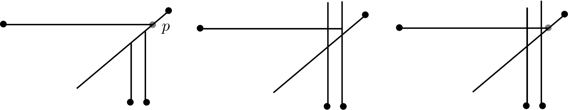
Figure 1. Black points are points of $\mathcal{P}$. From left to right: an iterated Gilbert process of order $k=1,2$ and $3$, respectively. Note that $p\in\mathcal{G}^{1}$ and $p\in\mathcal{G}^{3}$ but $p\notin\mathcal{G}^{2}$.

Below we will always make the no-parallel-line assumption: there exist at least two angles $\phi,\psi\in A$, $\phi\neq-\psi$, such that with positive probability, there are motorcycles that travel in this direction. This assumption is meant to rule out the trivial case where all motorcycles travel in parallel to each other, and then clearly their paths are of infinite lengths.

Proposition 3.

Under the no-parallel-line assumption, for all $k\geq 1$, $\mathcal{G}^{k}(\mathcal{P},\mathcal{A})$ is a well-defined random closed set.

Proof.

For a motorcycle $\bar{a}=(a,\phi)$, let $L^{k}(\bar{a})$ denote the length of its path from its origin to its grave in $\mathcal{G}^{k}(\mathcal{P},\mathcal{A})$. Let $\bar{\mathcal{P}}$ denote the marked point process consisting of ground points $\mathcal{P}$ and independent marks defined by $\mathcal{A}$. The goal is to show that $L^{k}$ is an exponentially stabilizing functional of $\bar{\mathcal{P}}$. That is, for each $\bar{a}$, there exists an a.s. finite random variable $R(\bar{a},\bar{\mathcal{P}})\in\mathbb{R}_{\geq 0}$ such that $L^{k}(\bar{a})$ is a finite random variable only depending on the points of $\bar{\mathcal{P}}$ which are inside a ball centered at $a$ and with radius $R(\bar{a},\bar{\mathcal{P}})$. In addition, the tail of the random variable $R(\bar{a},\bar{\mathcal{P}})$ is exponential. This in turn implies that the union of the edges in $\mathcal{G}^{k}$ is a well-defined random closed set in $\mathbb{R}^{2}$ in view of the fact that the support of $\mathcal{P}$ has no finite accumulation points.

Schreiber and Soja [17] proved this statement for the classical Gilbert process [17, Theorem 4]. Their proof only requires a small modification to adapt to this general setting. Indeed, consider a marked point $\bar{a}$. The crux of the proof for $k=1$ is to show that there exists a positive probability $\epsilon>0$ such that the motorcycle has its grave in the unit ball $B(a,1)$, or equivalently $\mathbb{P}(L^{1}(\bar{a})>1)\leq(1-\epsilon)$. Inside $B(a,1)$, choose a region $D$ such that, regardless of the configuration of points outside $B(a,1)$,

• for each $b\in D$, there exists a positive probability $\epsilon_{1}>0$ such that the motorcycle $\bar{b}=(b,\psi)$ whose random direction $\psi$ is sampled according to $\mathcal{A}$ kills $a$ in the event $E$ that disregarding multiplicity, $a,b$ are the only two points of $\mathcal{P}$ in $B(a,1)$, and

• $D$ has positive area, so with probability $\epsilon_{2}>0$, event $E$ holds.

Since the set of angles $A$ is finite, the angles at different points are chosen independently, and by the assumption which rules out parallel lines, the desired region $D$ exists. Then, with probability $\epsilon=\epsilon_{1}\epsilon_{2}>0$, the motorcycle $\bar{a}$ is killed by some motorcycle $\bar{b}$ with $b\in D$ and appropriate travel angle. Consider now non-overlapping and contiguous balls of radius 1 along the half line of apex $a$ and direction $\phi$. Define $N$ to be the first integer such that the ball $B(x+2N,1)$ contains a single marked point $\bar{b}$ in $D+2N$ with an appropriate angle such that $\bar{b}$ would kill $\bar{a}$ if latter is still alive by the time they are supposed to meet. Set our stabilizing radius $R(\bar{x},\bar{\mathcal{P}})=2N+1$. By the independence property of $\mathcal{P}$, one has $\mathbb{P}(R>n)\leq(1-\epsilon)^{n}$, and this supplies the finiteness and the exponential decaying behavior needed.

Now consider the case $k>1$. Let $N$ now denote the smallest integer such that there are $k$ ball with the appropriate single point property in the sequence of balls $B(x+2N,1)$. Clearly $2N+1$ is a stabilizing radius with an exponential tail. $\Box$

We have sacrificed generality for readability in Definition 1. Indeed, one can do away with several of our initial assumptions on $\mathcal{P},\mathcal{A}$ and $\mathcal{M}$, and Proposition 3 still holds by the same proof. In Section 3.2, we explore a non-trivial extension where at time $t=0$, there are obstacles in $\mathbb{R}^{2}$.

2.1. Iterated Gilbert Mosaic

In this paper, we shall focus on models where $\mathcal{G}^{k}(\mathcal{P},\mathcal{A})$ is a random mosaic. This is a countable system of compact, convex polygons that covers $\mathbb{R}^{2}$, with mutually no common interior points. Such a random mosaic can be identified with a tuple of point processes consisting of the centroids of its facets, edges and vertices. Applications of Campbell’s formula and Euler’s formula allow one to do computations on the statistics of random mosaics, see [16, §10].

Proposition 4.

Consider an iterated Gilbert model $\mathcal{G}^{k}=\mathcal{G}^{k}({\mathcal{P}},\mathcal{A})$ that satisfy the no-parallel-line assumption, and furthermore,

• (no isolated sites): $\mathcal{A}^{1}$ has total measure 0;

• (convex sites): for a supported value $2\leq m\leq M$, the joint angle distribution $\mathcal{A}^{m}$ is such that the absolute value of an angle formed between adjacent lines is less than or equal to $\pi$.

Then for $k\geq 1$, $\mathcal{G}^{k}$ is a random mosaic of the plane.

Proof.

By Proposition 3, $\mathcal{G}^{k}$ is a well-defined random closed set of $\mathbb{R}^{2}$. We say that two points of $\mathbb{R}^{2}\setminus\mathcal{G}^{k}$ are connected if there is a finite continuous path between them that does not intersect $\mathcal{G}^{k}$. This is an equivalence relation on $\mathbb{R}^{2}\setminus\mathcal{G}^{k}$. The equivalence classes are open sets which we will call cells. We need to show that cells are a.s. relatively compact and convex, and that their closures cover $\mathbb{R}^{2}$. As a random closed set, $\mathcal{G}^{k}$ consists of a.s. finite line segments. As there are no accumulation points in $\mathcal{P}$, only finitely many segments intersect any given compact set. So the closures of the cells of $\mathcal{G}^{k}$ cover $\mathbb{R}^{2}$, and furthermore, locally at each vertex, the cell is a polygon. We now prove convexity. Suppose for contradiction that there exists a cell of $\mathcal{G}^{k}$ that is not convex. As it is locally a polygon, it has a vertex with interior angle greater than $\pi$. We claim that a.s. no such vertices exist in $\mathcal{G}^{k}$. Indeed, a point of $\mathcal{G}^{k}$ is a vertex of some cell if and only if it is a point of $\mathcal{P}$, or it is a location where some motorcycle hits the line of another. In the former case, by the (no isolated sites) and (convex sites) assumptions, the interior angle is at most $\pi$. In the later case, since $\mathcal{P}$ is in general position, at least one motorcycle must continue after the collision, thus the point lies in the relative interior of at least one of the two lines. So the interior angle is also at most $\pi$. This proves the claim. Therefore, all facets of $\mathcal{G}^{k}$ are a.s. convex. Finally, we prove compactness. Let $F$ be a facet of $\mathcal{G}^{k}$. Let $F^{\prime}$ be the polygon obtained by removing all vertices of $F$ with flat interior angles. The edges of $F^{\prime}$ must be parallel to one of the angles in $A$. Since $F^{\prime}$ is a convex polygon, it can contain at most two edges with the same angle. But there are $M$ different angles, thus $F^{\prime}$ has at most $2M$ edges. Since the points of $\mathcal{P}$ are in general position, each edge of $F^{\prime}$ is a.s. generated by one motorcycle. Thus, the length of an edge in $F^{\prime}$ is at most the distance that this motorcycle travels in $\mathcal{G}^{k}$ before dying. The later is a.s. finite by Proposition 3. So $F^{\prime}$ is a.s. compact. Thus, $F$ is a.s. compact. $\Box$

A mosaic is said to be face-to-face if the facets form a cell complex, that is, the boundaries of facets have mutually no common interior points. Our iterated Gilbert model above is not face-to-face: an edge may terminate at an interior point of another edge. This issue is simple to resolve: one simply counts such interior points as vertices of the new edge, and define an edge as the line segment between two vertices, as before. This allows vertices with flat (180 degree) angles, and consecutive edges which are parallel to each other. This operation is called a face-to-face refinement. We can now define the central object of our study, the iterated Gilbert mosaic.

Definition 5.

An iterated Gilbert mosaic is the face-to-face refinement of an iterated Gilbert model $\mathcal{G}^{k}=\mathcal{G}^{k}({\mathcal{P}},\mathcal{A})$ that satisfies the assumptions of Proposition 4.

Definition 6.

For $k\geq 1$, say that a vertex $v$ of $\mathcal{G}^{k}$ is a site if $v\in\mathcal{P}$, and an intersection if $v$ is the intersection of a line with another line.

Proposition 7.

Let $\mathcal{G}^{k}=\mathcal{G}^{k}({\mathcal{P}},\mathcal{A})$ be an iterated Gilbert mosaic. Let $\mathbb{E}\mathcal{M}$ denote the mean multiplicity at a point in $\mathbb{P}$. For all $k\geq 1$, let $\lambda^{k}_{0},\lambda^{k}_{1},\lambda^{k}_{2}$ denote the (possibly infinite) intensities of the vertex, edge and facet processes of $\mathcal{G}^{k}$. Then

$$\lambda^{k}_{0} =(1+k)(\mathbb{E}\mathcal{M})\lambda,$$

$$\lambda^{k}_{1} =\frac{(\mathbb{E}\mathcal{M})+4k-1}{2}(\mathbb{E}\mathcal{M})\lambda,$$

$$\lambda^{k}_{2} =\frac{(\mathbb{E}\mathcal{M})+2k-3}{2}(\mathbb{E}\mathcal{M})\lambda.$$

In particular, $\mathcal{G}^{k}$ has all its facet sub-processes with finite intensity.

Proof.

First consider $k=1$. Vertices of $\mathcal{G}^{1}$ are either sites or intersections. The intensity of sites is $\lambda(\mathbb{E}\mathcal{M})$. Each intersection corresponds to precisely one death event of a motorcycle. Since each motorcycle dies exactly once, the intensity of intersections is also $\lambda(\mathbb{E}\mathcal{M})$. Thus $\lambda^{1}_{0}=2(\mathbb{E}\mathcal{M})\lambda$. Now consider the edge process of $\mathcal{G}^{1}$. For this, we use a mass transport argument. Construct a directed graph $G$ as follows: the vertices of this graph are the vertices of $\mathcal{G}^{1}$ and the centroids of the edges of $\mathcal{G}^{1}$. From each edge centroid, put a directed edge to each of the two vertices of this edge. Note that $G$ is a bipartite graph, from the set of edges of $\mathcal{G}^{1}$ to the set of vertices of $\mathcal{G}^{1}$. As each edge of $\mathcal{G}^{1}$ generates precisely two directed edges, the mean out-degree $\delta_{out}$ of $G$ is

$$\delta_{out}=2\lambda_{1}^{1}.$$

Now consider the mean in-degree of $G$. Each site in $\mathcal{G}^{1}$ contributes a mean in-degree of $(\mathbb{E}\mathcal{M})$. Each intersection contributes an in-degree of 3, by general positioning of the points in ${\mathcal{P}}$. Therefore, the mean in-degree $\delta_{in}$ of the graph $G$ is

$$\delta_{in}=(\mathbb{E}\mathcal{M})(\mathbb{E}\mathcal{M})\lambda+3(\mathbb{E}\mathcal{M})\lambda=(3+(\mathbb{E}\mathcal{M}))(\mathbb{E}\mathcal{M})\lambda.$$

The mass transport principle says that $\delta_{in}=\delta_{out}$. Hence $\lambda_{1}^{1}=\frac{3+(\mathbb{E}\mathcal{M})}{2}(\mathbb{E}\mathcal{M})\lambda$ as claimed. We use the same argument to derive the formula for $\lambda_{2}^{1}$. Construct a directed graph $G^{\prime}$ as follows: the vertices of this graph are the vertices of $\mathcal{G}^{1}$ and the centroids of the facets of $\mathcal{G}^{1}$. From each facet centroid, put a directed edge to each of the vertices of this facet. Note that $G^{\prime}$ is a bipartite graph, from the set of edges of $\mathcal{G}^{1}$ to the set of vertices of $\mathcal{G}^{1}$. The mean in-degree of $G^{\prime}$ is

$$\delta_{in}=\delta\lambda_{2}^{1}$$

for some constant $\delta>0$, interpreted as the mean number of vertices per face of $\mathcal{G}^{1}$. Now consider the mean out-degree $\delta_{out}$ of $G^{\prime}$. For a vertex of $\mathcal{G}^{1}$, the number of faces with this vertex equals the number of edges at this vertex. So the mean in-degree of $G^{\prime}$ equals to the mean in-degree of $G$, which is

$$\delta_{in}=(3+(\mathbb{E}\mathcal{M}))(\mathbb{E}\mathcal{M})\lambda.$$

By the mass transport principle,

$$(3+(\mathbb{E}\mathcal{M}))(\mathbb{E}\mathcal{M})\lambda=\delta\lambda_{2}^{1}.$$

Since $(\mathbb{E}\mathcal{M}),\lambda<\infty$, the quantities on the right-hand side must also be finite. This implies that $\mathcal{G}^{k}$ is a random mosaic with finite intensity. By the Euler characteristic formula [16, Equation 14.63],

$$\lambda_{2}^{1}=\lambda_{1}^{1}-\lambda_{0}^{1}.$$

Rearranging gives the formula for $\lambda_{2}^{1}$. The case of general $k$ is similar. Here a motorcycle dies precisely $k$ times, hence $\lambda_{0}^{k}=(k+1)(\mathbb{E}\mathcal{M})\lambda$. Note that each motorcycle has one final death event, which corresponds precisely to one intersection of degree 3. For all other collisions, the two motorcycles involved will continue, creating vertices of intersection of degree 4. Thus, each motorcycle creates $k-1$ vertices with multiplicity 4, and $1$ vertex with multiplicity $3$. This implies the equation

$$2\lambda_{1}^{k}=(\mathbb{E}\mathcal{M})(\mathbb{E}\mathcal{M})\lambda+4(k-1)(\mathbb{E}\mathcal{M})\lambda+3(\mathbb{E}\mathcal{M})\lambda=(4k-1+(\mathbb{E}\mathcal{M}))(\mathbb{E}\mathcal{M})\lambda.$$

Finally, for the facets, by the Euler characteristic formula,

$$\lambda_{2}^{k}=\lambda_{1}^{k}-\lambda_{0}^{k}=\frac{(\mathbb{E}\mathcal{M})+2k-3}{2}(\mathbb{E}\mathcal{M})\lambda.$$

$\Box$

Corollary 8.

Let $\mathcal{G}^{k}=\mathcal{G}^{k}({\mathcal{P}},\mathcal{A})$ be an iterated Gilbert mosaic. Let $\mathbb{E}\mathcal{M}$ denote the mean multiplicity at a point in $\mathcal{P}$. Then the mean number of vertices per face of $\mathcal{G}^{k}$ is $2\lambda(\mathbb{E}\mathcal{M})\frac{(\mathbb{E}\mathcal{M})+4k-1}{(\mathbb{E}\mathcal{M})+2k-3}$.

3. Scaling limits of iterated Gilbert mosaics

Let $\mathcal{G}^{k}$ be an iterated Gilbert mosaic. We want to know if there exists a sequence $f(k)$ such that when taking for the intensity of $\mathcal{P}$ $\frac{\lambda}{f(k)}$ rather than $\lambda$, $\mathcal{G}^{k}$ converges (in some sense) to a non-trivial limiting random mosaic. Proposition 7 suggests that one should take $f(k)=k$ to see non-trivial limits. Our main result, Theorem 10, states that at this scaling, the limit in the vague topology is a Poisson line process with a particular measure. To state this limiting measure, we first need some definitions.

For $w=\{w_{\phi}\in\mathbb{R}_{\geq 0}:\phi\in A\}$, view $w$ as a vector in $\mathbb{R}^{M}$ with non-decreasing coordinates, that is, $w_{1}\leq\ldots\leq w_{M}$. For a pair $\phi,\varphi\in A$, let $T^{w_{\phi},w_{\varphi}}_{\phi\varphi}\subset\mathbb{R}^{2}$ be the polygon with vertex set

$$\mathsf{vertex}(T^{w_{\phi},w_{\varphi}}_{\phi\varphi})=\left\{\begin{array}[]{cc}\{(0,0),-w_{\varphi}\cdot\overrightarrow{\varphi},-w_{\phi}\cdot\overrightarrow{\phi},(w_{\varphi}-w_{\phi})\cdot\overrightarrow{\phi}-w_{\varphi}\cdot\overrightarrow{\varphi}\}&\mbox{ if }w_{\varphi}<w_{\phi},\\ \{(0,0),-w_{\phi}\cdot\overrightarrow{\varphi},-w_{\phi}\cdot\overrightarrow{\phi}\}&\mbox{ else.}\end{array}\right.$$

That is, $T^{w_{\phi},w_{\varphi}}_{\phi\varphi}$ is a triangle with side lengths $w_{\phi}$ if $w_{\varphi}\geq w_{\phi}$, and otherwise, it is the trapezium obtained by truncating a piece off the triangle with side lengths $w_{\varphi}$. Note that $T^{w_{\phi},w_{\varphi}}_{\phi\varphi}\neq T^{w_{\varphi},w_{\phi}}_{\varphi\phi}$ unless if $w_{\phi}=w_{\varphi}$. See Figure 2 for an illustration.

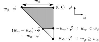
Figure 2. The polygon $T^{w_{\phi},w_{\varphi}}_{\phi\varphi}$ illustrated for the two directions $\vec{\varphi}=(0,1)$ and $\vec{\phi}=(1,0)$. If $w_{\varphi}<w_{\phi}$, then $T^{w_{\phi},w_{\varphi}}_{\phi\varphi}$ is the shaded trapezium. If $w_{\varphi}\geq w_{\phi}$, then $T^{w_{\phi},w_{\varphi}}_{\phi\varphi}$ is the entire triangle, that is, the trapezium union with the white small triangle at the bottom. For $\bar{b}=(b,\phi)$, $\tau_{b}\circ T^{w_{\phi},w_{\varphi}}_{\phi\varphi}$ is the polygon translated so that the vertex $-w_{\phi}\cdot\vec{\phi}$ is at $b$.

For all $\phi\in A$, define

$$\mathcal{E}(w,\phi)=\sum_{Q\subseteq A\setminus\{\phi\}}\sum_{\varphi\in Q}|T^{w_{\phi},w_{\varphi}}_{\phi\varphi}|(\mu_{\phi\cup Q}+\mu_{Q}),$$ (1)

where we recall that $\mu_{Q}$ denotes the intensity of sites in $\mathcal{P}$ with set of angles $Q$. Assume that each motorcycle $\bar{a}=(a,\varphi)$ travels a distance of exactly $w_{\varphi}$; then $\mathcal{E}(w,\phi)$ is the mean number of motorcycle trajectories that motorcycle $\bar{b}=(b,\phi)$ crosses on $[b,b+w_{\phi}\vec{\phi}]$ such that $\bar{b}$ does not come first at this intersection, see Figure 3. The two terms $\mu_{\phi\cup Q}$ and $\mu_{Q}$ take into account the fact that motorcycle $\bar{b}$ crosses trajectories stemming from sites with angle set containing $\phi$ as well as from sites not containing $\phi$.

In addition to (1), it is sometimes convenient to consider another formula for $\mathcal{E}(w,\phi)$. For each $S\subset A\setminus\{\phi\}$, define

$$T^{w}_{\phi S}:=\left(\bigcap_{\varphi\in S}T^{w_{\phi},w_{\varphi}}_{\phi\varphi}\right)\backslash\left(\bigcup_{{Q^{\prime}\supset S}\atop{Q^{\prime}\neq S}}\bigcap_{\varphi^{\prime}\in Q^{\prime}}T^{w_{\phi},w_{\varphi^{\prime}}}_{\phi\varphi^{\prime}}\right)\subset\mathbb{R}^{2}.$$ (2)

Then one can rewrite $\mathcal{E}(w,\phi)$ as

$$\mathcal{E}(w,\phi)=\sum_{Q\subseteq A\backslash\{\phi\}}(\mu_{\phi\cup Q}+\mu_{Q})\sum_{S\subseteq Q}|S||T^{w}_{\phi S}|.$$ (3)

The advantage of the last formulation is that by definition, the sets $T^{w}_{\phi S}$ are mutually disjoint. So $\mathcal{E}(w,\phi)$ is the expected value of the weighted sum of independent Poisson random variables

$$\sum_{Q\subseteq A\backslash\{\phi\}}\sum_{S\subseteq Q}|S|(\mathcal{P}_{\phi\cup Q}\left(T^{w}_{\phi S})+\mathcal{P}_{Q}(T^{w}_{\phi S})\right).$$

Figure 3. Illustration of Formula (1). Left: the set of angles depicted with the distances $w$. Right: the three associated regions. Here, $\mathcal{E}(w,\phi)$ is the average number of sites of $\mathcal{P}$ which contains a motorcycle $\bar{a}=(a,\varphi)$, $\varphi\neq\phi$, that comes first at their meeting with $\bar{b}=(b,\phi)$ on $[b,b+w_{\phi}\vec{\phi}]$. Note that points $T_{\phi\varphi_{1}}\cap T_{\phi\varphi_{2}}$ are counted twice in the sum. Regroup the sum by the mutually disjoint intersected regions, weighted by their multiplicities, gives (3).

Consider now the iterated Gilbert model and the distance a typical motorcycle $\bar{a}=(a,\varphi)$ can travel with $k$ lives. Assuming that this distance is concentrated around some mean value $w^{\ast}_{\varphi}\sqrt{k}$ for all $\varphi$, the vector $w^{\ast}\in\mathbb{R}^{M}$ should satisfy the relation

$$\mathcal{E}(w^{\ast}_{\phi}\sqrt{k},\phi)=k,\mbox{ for all }\phi\in A.$$ (4)

Lemma 9.

There exists a unique set of positive constants $w^{\ast}=\{w^{\ast}_{\phi}\in\mathbb{R}_{\geq 0}:\phi\in A\}$ that satisfies (4) for all $k>0$.

Proof.

Since $|T^{k\cdot w}_{\phi Q}|=k^{2}|T^{w}_{\phi Q}|$ for any $k>0$, for any set of constants $w=\{w_{\phi}\}$,

$$\frac{\mathcal{E}(w_{\phi}\sqrt{k},\phi)}{k}=\mathcal{E}(w_{\phi},\phi)\mbox{ for each }\phi\in A.$$

So one just needs to show that there exists a unique set of constants $w^{\ast}$ such that

$$\mathcal{E}(w^{\ast}_{\phi},\phi)=1\mbox{ for all }\phi\in A.$$

Consider the map $\mathbb{R}_{\geq 0}\to\mathbb{R}_{\geq 0}^{M}$, $c\mapsto(\mathcal{E}(c\cdot\mathbf{1},\phi),\phi\in A)$. This map is continuous, increasing and tends to infinity in each of its coordinates. Thus, there exists a unique constant $w^{\ast}_{1}\in\mathbb{R}_{\geq 0}$ such that

$$\max_{\phi\in A}\mathcal{E}(w^{\ast}_{1}\cdot\mathbf{1},\phi)=1.$$ (5)

Let $\phi_{1}\in A$ be an angle that achieves this maximum, that is,

$$\mathcal{E}(w^{\ast}_{1}\cdot\mathbf{1},\phi_{1})=1.$$

It follows from the definition of $\mathcal{E}$ (and more precisely the trapezium structure when $\varphi>\phi$ in the definition of $T^{w_{\phi},w_{\varphi}}_{\phi\varphi}$), that if $w=\{w_{\phi}\}$ is such that $w_{\phi_{1}}=w^{\ast}_{1}$, and $w_{\varphi}\geq w^{\ast}_{1}$ for all $\varphi\in A$, then

$$\mathcal{E}(w,\phi_{1})=1.$$

So now, let $\mathbf{1}^{(-1)}\in\mathbb{R}^{M}$ be the all-one vector, except in the coordinate corresponds to $\phi_{1}$, where it is $0$. For $c\geq 0$, the map $\mathbb{R}_{\geq 0}\to\mathbb{R}_{\geq 0}^{M}$, $c\mapsto(\mathcal{E}(w^{\ast}_{1}\cdot\mathbf{1}+c\cdot\mathbf{1}^{(-1)}\},\phi),\phi\in A)$ is constant in the coordinate corresponds to $\phi_{1}$, while in other coordinates, it is continuous, monotone increasing, with starting value at most 1. Thus, there exists a unique constant $w_{2}^{\ast}\geq w_{1}^{\ast}$ such that

$$\max_{\phi\in A\backslash\{\phi_{1}\}}\mathcal{E}(w^{\ast}_{1}\cdot\mathbf{1}+(w^{\ast}_{2}-w^{\ast}_{1})\cdot\mathbf{1}^{(-1)}\},\phi)=1,$$

and in particular, this maximum is achieved at some coordinate $\phi_{2}\in A\backslash\{\phi_{1}\}$. Repeat this argument, we obtain the unique $w^{\ast}$ needed. $\Box$

Let $\mathcal{G}^{k}\left(\frac{1}{k}\right)$ denote the the iterated Gilbert mosaic of order $k$ for the same angle distribution $\mathcal{A}$ as above, but for a Poisson point process with intensity multiplied by $\frac{1}{k}$. For all $R\subset\mathbb{R}^{2}$ and $u\in\mathbb{R}$, let $u\cdot R$ denote the set $\{ux,x\in R\}$. Note that since $\mathcal{P}$ is stationary, multiplying the intensity by $\frac{1}{k}$ is the same as rescaling space by $\sqrt{k}$ in the $x$ and $y$ axes. Hence $\mathcal{G}^{k}\left(\frac{1}{k}\right)$ is equal in distribution to $\sqrt{k}\cdot\mathcal{G}^{k}$, which will be used throughout in what follows.

Theorem 10.

Let $w^{\ast}$ be the unique set of constants in Lemma 9. Let $\mathcal{G}^{k}({\mathcal{P}},\mathcal{A})$ be an iterated Gilbert mosaic. As $k\to\infty$, for any compact window $W\subset\mathbb{R}^{2}$,

$$\mathcal{G}^{k}\left(\frac{1}{k}\right)\cap W\to\mathcal{G}^{\infty}\cap W\mbox{ in probability},$$

where $\mathcal{G}^{\infty}$ is a Poisson line process with cylindrical measure $\Lambda dr\times\Theta(d\theta)$, with $\Lambda$ the constant

$$\Lambda=\sum_{\phi\in A}w^{*}_{\phi}\sum_{Q\subset A,\phi\in Q}\mu_{Q}$$

and $\Theta$ the probability measure with mass

$$\frac{1}{\Lambda}w^{*}_{\phi}\sum_{Q\subset A,\phi\in Q}\mu_{Q}$$

at $\phi^{\perp}=\phi+\frac{\pi}{2}$ (recall that lines are parameterized by their point which is the closest to the origin, and that the angle of this point is $\phi^{\perp}$ if the line has angle $\phi$) for all $\phi\in A$, where $w^{\ast}$ is defined by (4).

Let us now explain qualitatively why the mosaics admit a scaling limit at a linear rate. As we saw in Proposition 7, the intersections of $\mathcal{G}^{k}$ densify at a linear rate with respect to $k$. Suppose we knew that the limit $\mathcal{G}^{k}\left(\frac{1}{k}\right)$ exists. Intuitively, the limiting process must be a classical Poisson line process. Then, the starting points of the motorcycles, which are points of $\mathcal{P}$, are getting further and further apart. A view of the process by a typical compact window $W$ consists of paths of the motorcycles, which are lines with directions in $A$. With high probability, these lines are independent, since they come from different, far-away starting points. Thus, the limiting process must be a classical Poisson line process. The difficulties are in working out the measure $\Theta$ precisely and in proving that the limit holds indeed.

We now state and prove the two auxiliary results, Propositions 11 and 12, used for the proof of Theorem 10. Fix $k\in\mathbb{N}$. For a motorcycle $\bar{b}=(b,\phi)$, recall that $L^{k}(\bar{b})$ is the length of the path from its origin to its grave in $\mathcal{G}^{k}$. Proposition 11 claims that for large $k$, $L^{k}(\bar{b})/\sqrt{k}$ concentrates around $w^{\ast}_{\phi}$, and this concentration holds simultaneously for all motorcycles whose starting points lie in some dilated compact set.

Proposition 11.

Fix a compact set $R\subset\mathbb{R}^{2}$. With probability $1-\epsilon(k,\phi)$ which approaches $1$ as $k\to\infty$,

$$\sup_{b\in\sqrt{k}\cdot R}\left|\frac{L^{k}((b,\phi))}{\sqrt{k}}-w^{\ast}_{\phi}\right|\leq o(1).$$

We defer the proof of Proposition 11 to the next section. The heart of the argument uses a Chernoff-type bound to control the supremum of a Poisson functional, and an induction on the sequence of angles of $A$, ordered such that the sequence of constants $w^{\ast}=(w^{\ast}_{\phi})$ is non-decreasing.

Now fix $\phi\in A$. Let $W\subset\mathbb{R}^{2}$ be a compact set. For $k\geq 1$, define $W_{k}:=\frac{1}{\sqrt{k}}\cdot W$. The second auxiliary result is Proposition 12 below, which claims that for large $k$, with overwhelming probability, motorcycles whose paths intersect $W_{k}$ in $\mathcal{G}^{k}$ must have their origins in a particular strip.

Proposition 12.

With probability $1-\epsilon^{\prime}(k,\phi)$ which approaches $1$ as $k\to\infty$, the path in $\mathcal{G}^{k}$ of a motorcycle $\bar{b}=(b,\phi)$ intersects $W_{k}$ if and only if

$$b\in R(\phi,k):=[\sqrt{k}w^{\ast}_{\phi}\cdot(-\overrightarrow{\phi}),(0,0)]\oplus W_{k},$$

where for all $C,D\subset\mathbb{R}^{M}$, $C\oplus D$ denotes the set $\{x+y,x\in C,y\in D\}$.

Proof.

Assume without loss of generality that $W$ is convex. Fix $k$. Let $\Pi_{\phi}W_{k}$, $\Pi_{\phi^{\perp}}W_{k}$ be the line segments obtained by projecting $W_{k}$ along $\phi$ and $\phi^{\perp}$, onto $\mathbb{R}\cdot\overrightarrow{\phi^{\perp}}$ and $\mathbb{R}\cdot\overrightarrow{\phi^{\perp}}$, respectively. Let $g_{k}$ and $d_{k}$ be the left-most and right-most points of $\Pi_{\phi^{\perp}}W_{k}$, that is,

$$g_{k} =\sup\{c\in\mathbb{R}:\langle w,\phi\rangle\geq c\mbox{ for all }w\in W_{k}\},$$

$$d_{k} =\inf\{c\in\mathbb{R}:\langle w,\phi\rangle\leq c\mbox{ for all }w\in W_{k}\}.$$

For $y>0$, let $R(y)$ be the translated segment $y\sqrt{k}\cdot(-\overrightarrow{\phi})+\Pi_{\phi}W_{k}-g_{k}$. Note that any $\bar{b}$ whose path intersects $W_{k}$ must have $b\in R(y)$ for some $y>g_{k}-d_{k}$. To prove the statement, it is sufficient to show that with high probability, the following events hold simultaneously (see Figure 4):

$$b\in R(y),0<y<w^{\ast}_{\phi}-o(1)\Rightarrow\mbox{ $\bar{b}$ hits $W_{k}$,}$$ (6)

$$b\in R(y),y>w^{\ast}_{\phi}+o(1)\Rightarrow\mbox{ $\bar{b}$ does not hit $W_{k}$,}$$ (7)

$$\mbox{ there are no motorcycles $b$ with $b\in R(y)$ for }w^{\ast}_{\phi}-o(1)\leq y\leq w^{\ast}_{\phi}+o(1)\mbox{ or }g_{k}-d_{k}\leq y\leq 0.$$ (8)

By Proposition 11, with probability at least $1-2\epsilon(k,\phi)$,

$$L^{k}(\bar{b}) >\sqrt{k}(w^{\ast}_{\phi}-o(1))\mbox{ for all }b\in R(w^{\ast}_{\phi}-o(1)),\mbox{ and }$$ (9)

$$L^{k}(\bar{b}) <\sqrt{k}(w^{\ast}_{\phi}+o(1))\mbox{ for all }b\in R(w^{\ast}_{\phi}+o(1)).$$ (10)

Now, consider shifting motorcycle $\bar{b}=(b,\phi)$ along $\overrightarrow{\phi}$ to a starting location $b^{\prime}$ closer to $W_{k}$, while keeping all other motorcycles the same. Clearly if $\bar{b}$ can hit $W_{k}$ from $b$, it also can hit $W_{k}$ from $b^{\prime}$. Thus, (9) implies (6). Similarly, if $b^{\prime}$ is further away from $W_{k}$, then if $\bar{b}$ cannot hit $W_{k}$ from $b$, it also cannot hit $W_{k}$ from $b^{\prime}$. Thus, (10) implies (7). Finally, as $W$ is compact, $|g_{k}-d_{k}|=O(k^{-1/2})$, so the last event (8) is contained in the event that there is no point of $\mathcal{P}$ in a region with area $o(1)$, so it happens with probability $1-\epsilon_{k}$ for $\epsilon_{k}\to 1$ as $k\to\infty$. So, with probability at least $1-2\epsilon(\phi,k)-\epsilon_{k}$, the desired events (6-8) hold. Choose $\epsilon^{\prime}(k,\phi)=2\epsilon(\phi,k)+\epsilon_{k}$, one obtains the desired result. $\Box$

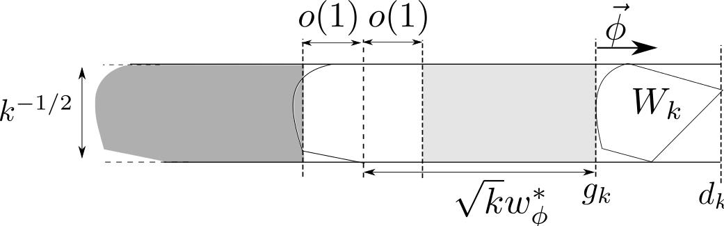
Figure 4. The cut-off phenomenon in Proposition 12 illustrated. With high probability, in $\mathcal{G}^{k}$, all points $\bar{b}=(b,\phi)$ with starting point $b$ in the light region will hit $W_{k}$, all those with $b$ in the dark region will not hit $W_{k}$, and there are no points in the white region.

Proof of Theorem 10.

Let $\{P_{\phi},\phi\in A\}$ be independent Poisson line processes, with $P_{\phi}$ consisting of lines parallel to $\overrightarrow{\phi}$, whose projection onto $\mathbb{R}\cdot\overrightarrow{\phi}^{\perp}$ form a Poisson point process with intensity $w^{*}_{\phi}\sum_{Q\subset A,\phi\in Q}\mu_{Q}$. Note that $\mathcal{G}^{\infty}=\bigcup_{\phi\in A}P_{\phi}$. By Proposition 12, as $k\to\infty$, the process of segments of $\mathcal{G}^{k}$ parallel to $\phi$ that intersect $\frac{1}{\sqrt{k}}W$ converges in probability to the process of lines of $P_{\phi}$ that intersect $W$. As $A$ is a finite set, by union bound over $A$, with high probability, the events in Proposition 12 hold simultaneously for all $\phi\in A$. Let

$$R^{\prime}(\phi,k)=R(\phi,k)\backslash\bigcup_{\varphi\in A,\varphi\neq\phi}\left(R(\phi,k)\cap R(\varphi,k)\right).$$

Since $W$ is compact, the pairwise intersections $R(\phi,k)\cap R(\varphi,k)$ has area of order $O(k^{-1/2})$, while $R(\phi,k)$ has area of order $O(1)$. So with high probability, $\mathcal{P}\cap R(\phi,k)=\mathcal{P}\cap R^{\prime}(\phi,k)$ for all $\phi\in A$. Since the regions $R^{\prime}(\phi,k)$ are pairwise disjoint, the lines intersecting $\frac{1}{\sqrt{k}}W$ in $\mathcal{G}^{k}$ converges in probability to the intersection of $W$ and $\mathcal{G}^{\infty}$. That is,

$$\lim_{k\to\infty}\mathcal{G}^{k}\cap\frac{1}{\sqrt{k}}W\stackrel{{\scriptstyle P}}{{\to}}\mathcal{G}^{\infty}\cap W.$$

As $\mathcal{G}^{k}$ is stationary, this implies

$$\lim_{k\to\infty}\mathcal{G}^{k}\left(\frac{1}{k}\right)\cap W\stackrel{{\scriptstyle P}}{{\to}}\mathcal{G}^{\infty}\cap W,$$

and this concludes the proof of Theorem 10. $\Box$

3.1. Proof of Proposition 11

The proof is organized in a series of lemmas. We start with a concentration result on Poisson point processes to be used in the proofs.

Lemma 13.

Let $\mathcal{P}_{k}$ be a PPP with rate $k\lambda$. Let $R,S\subset\mathbb{R}^{2}$ be compact sets. Assume that $S$ has finite boundary, that is, $|S^{t}\backslash S|=O(t)$ as $t\to 0$, with $S^{t}=\{x\in\mathbb{R}^{2}:\|x-S\|_{\infty}\leq t\}$ where $\|y\|_{\infty}:=\max\{|y_{1}|,|y_{2}|\}$ is the $L_{\infty}$-norm in $\mathbb{R}^{2}$. For $a\in R$, let $N_{k}(a)=\mathcal{P}_{k}(S+a)$ be the number of points of $\mathcal{P}_{k}$ in the set $S+a$. For any fixed $\epsilon>0$, as $k\to\infty$, with high probability,

$$\sup_{a\in R}\left|N_{k}(a)-k\lambda|S|\right|\leq O(\lambda|S|k^{1/2+\epsilon}).$$

In other words, with high probability,

$$k\lambda|S|+O(\lambda|S|k^{1/2+\epsilon})\leq\inf_{a\in R}N_{k}(a)\leq\sup_{a\in R}N_{k}(a)\leq k\lambda|S|+O(\lambda|S|k^{1/2+\epsilon}).$$

Proof.

The proof is a union bound over a $\delta$-net. Let $X$ be a Poisson random variable with mean $k\mu$. By Chernoff’s bound for Poisson random variables, for $\epsilon>0$, there exists a constant $C>0$ such that

$$\mathbb{P}(|X-k\mu|\geq(k\mu)^{1/2+\epsilon})\leq\exp(-C(k\mu)^{2\epsilon}).$$

Set $X=N_{k}$ with $\mu=\lambda|S|$. Cover $R$ by a grid where each square has side length at most $\delta=k^{-2}$. Let $G$ be the set of center points of squares which have non-empty intersection with $R$. Associate to each point $a\in R$ the center $g(a)\in G$ of the square it belongs to (squares can be taken closed on the left/bottom and open on the right/top to avoid ties). Then, a.s.,

$$\sup_{a\in R}\left|N_{k}(a)-k\mu\right| \leq\sup_{a\in R}\left(\left|N_{k}(a)-N_{k}(g(a))\right|+\left|N_{k}(g(a))-k\mu\right|\right)$$

$$\leq\sup_{g\in G}\sup_{a:\|a-a_{G}\|_{\infty}<\delta/2}\left|N_{k}(a)-N_{k}(g)\right|+\left|N_{k}(g)-k\mu\right|.$$ (11)

Since $\|a-g\|_{\infty}<\delta/2$, we have $S^{\delta}+a_{G}\supseteq S+a$. Let $N_{k}^{\delta}(a_{G})=|\mathcal{P}_{k}\cap(S^{\delta}+a_{G})|$. Then

$$\sup_{a:\|a-a_{G}\|_{\infty}<\delta/2}\left|N_{k}(a)-N_{k}(a_{G})\right|\leq N_{k}^{\delta}(a_{G})-N_{k}(a_{G})=|\mathcal{P}_{k}\cap(S^{\delta}\backslash S+a_{G})|.$$

So $N_{k}^{\delta}(a_{G})-N_{k}(a_{G})$ is a Poisson random variable with mean at most $C^{\prime}k\lambda\delta$ for some constant $C^{\prime}>0$, thanks to the assumption on the boundary. The cardinality of $G$ is at most $2|R|\delta^{-2}$. So by the union bound,

$$\mathbb{P}(\sup_{a_{G}\in G}N_{k}^{\delta}(a_{G})-N_{k}(a_{G})>0)\leq 2|R|\delta^{-2}(1-\exp(-C^{\prime}k\lambda\delta))=O(k/\delta)=O(k^{-1}),$$

and

$$\mathbb{P}(\sup_{a_{G}\in G}\left|N_{k}(a_{G})-k\mu\right|\geq(k\mu)^{1/2+\epsilon})\leq 2|R|\delta^{-2}\exp(-C(k\mu)^{2\epsilon})=\exp(-O(k^{2\epsilon})+4\log k).$$

This together with the bound (11) imply that w.h.p.

$$\sup_{a\in R}\left|N_{k}(a)-k\mu\right|\leq\sup_{a_{G}\in G}(N_{k}^{\delta}(a_{G})-N_{k}(a_{G}))+\sup_{a_{G}\in G}\left|N_{k}(a_{G})-k\mu\right|\leq(k\mu)^{1/2+\epsilon}=O(k^{1/2+\epsilon}).$$

$\Box$

Below is another auxiliary result, which are bounds on the function $w\mapsto\mathcal{E}(w,\phi)$ under small perturbations. They follow from the geometry of the regions $T^{w}_{\phi Q}$.

Lemma 14.

Fix $i\in\{1,\ldots,M\}$. Fix a sequence of constants $0<\delta_{1}\leq\ldots\leq\delta_{i-1}<\delta_{i}\leq\delta_{i+1}\leq\ldots\leq\delta_{M}$. Define weight vectors $w,w^{\prime}\in\mathbb{R}^{M}$ with

$$w_{\ell}=w^{\ast}_{\ell}+k^{\delta_{\ell}}\mbox{ for }\ell=1,\ldots,i-1,\hskip 10.00002ptw_{\ell}=w^{\ast}_{i}-k^{\delta_{i}}\mbox{ for }\ell\geq i,$$

and

$$w^{\prime}_{\ell}=w^{\ast}_{\ell},\mbox{ for }\ell=1,\ldots,i-1,\hskip 10.00002ptw^{\prime}_{\ell}=w^{\ast}_{i},\mbox{ for }\ell\geq i.$$

Then for $j>i$,

$$\mathcal{E}(w,\phi_{j})=\mathcal{E}(w^{\prime},\phi_{j})+o(k^{\delta_{i}})-Ck^{\delta_{i}}$$

for some constant $C>0$. Similarly, if

$$w_{\ell}=w^{\ast}_{\ell}-k^{\delta_{\ell}}\mbox{ for }\ell=1,\ldots,i-1,\hskip 10.00002ptw_{\ell}=w^{\ast}_{i}+k^{\delta_{i}}\mbox{ for }\ell\geq i,$$

then for $j>i$,

$$\mathcal{E}(w,\phi_{j})=\mathcal{E}(w^{\prime},\phi_{j})-o(k^{\delta_{i}})+Ck^{\delta_{i}}$$

for some constant $C>0$.

Proof.

Consider the difference $|T^{w}_{\phi_{j}Q}|-|T^{w^{\prime}}_{\phi_{j}Q}|$ for each subset $Q\subseteq A\backslash\{\phi_{j}\}$. For coordinates $\ell<i$, $w_{\ell}-w^{\prime}_{\ell}=k^{\delta_{\ell}}=o(k^{\delta_{i}})$, and thus this contributes a positive term of order $o(k^{\delta_{i}})$ to this difference. Now consider coordinates $\ell\geq i$. Then $w_{\ell}-w^{\prime}_{\ell}=-k^{\delta_{i}}$, and thus this contributes a negative term of order $O(k^{\delta_{i}})$. Sum over all such subsets $Q$ and use (3) to obtain

$$\mathcal{E}(w,\phi_{j})-\mathcal{E}(w^{\prime},\phi_{j})=o(k^{\delta_{i}})-Ck^{\delta_{i}}$$

for some constant $C>0$. The second part follows similarly. $\Box$

Fix $k\in\mathbb{N}$, a motorcycle $\bar{b}=(b,\phi)$, with $b\in\sqrt{k}\cdot R$, some distance $y>0$, and angle $\varphi\in A,\varphi\neq\phi$. Write $K(\bar{b},y,\varphi,k)$ for the number of would-be killers of $\bar{b}$ on $b+[0,y\sqrt{k}\cdot\overrightarrow{\phi}]$ which travel in direction $\varphi\in A$. That is, these are motorcycles $\bar{a}=(a,\varphi)$ whose path in $\mathcal{G}^{k}$ would cross $b+[0,y\sqrt{k}\cdot\overrightarrow{\phi}]$, and $\bar{a}$ would have killed $\bar{b}$ if $\bar{b}$ had enough lives to meet it, which will happen for large enough $k$. Our goal is to give a tight bound of the kind

$$\underline{K}(\bar{b},y,\varphi,k)\leq K(\bar{b},y,\varphi,k)\leq\overline{K}(\bar{b},y,\varphi,k)\hskip 10.00002pt\mbox{for all $b\in\sqrt{k}\cdot R$, w.h.p.,}$$ (12)

for some appropriately defined $\underline{K}$ and $\overline{K}$. Summing over $\varphi\in A\backslash\{\phi\}$ and taking a union bound, one obtains upper and lower bounds for the number of would-be killers $K(\bar{b},y,k)$ of $b$ on $b+[0,y\sqrt{k}\cdot\overrightarrow{\phi}]$,

$$\underline{K}(\bar{b},y,k)\leq K(\bar{b},y,k)\leq\overline{K}(\bar{b},y,k)\hskip 10.00002pt\mbox{for all $b\in\sqrt{k}\cdot R$, w.h.p.},$$

where

$$\underline{K}(\bar{b},y,k) :=\sum_{\varphi\in A\backslash\{\phi\}}\underline{K}(\bar{b},y,\varphi,k)$$ (13)

$$K(\bar{b},y,k) :=\sum_{\varphi\in A\backslash\{\phi\}}K(\bar{b},y,\varphi,k),$$ (14)

$$\overline{K}(\bar{b},y,k) :=\sum_{\varphi\in A\backslash\{\phi\}}\overline{K}(\bar{b},y,\varphi,k).$$ (15)

The definitions of the quantities $\underline{K}(\bar{b},y,\varphi,k)$ and $\overline{K}(\bar{b},y,\phi,k)$ are given below, depending on whether $w^{\ast}_{\phi}$ or $w^{\ast}_{\varphi}$ is greater. Let us motivate these definitions. For $b\in\mathbb{R}^{2}$, let $\tau_{b}\circ T^{w_{\phi},w_{\varphi}}_{\phi\varphi}$ be the polygon $T^{w_{\phi},w_{\varphi}}_{\phi\varphi}$ translated so that the vertex $-w_{\phi}\cdot\overrightarrow{\phi}$ is now at $b$. Say that $\bar{a}=(a,\varphi)$ is a potential killer of $\bar{b}$ in direction $\varphi$ on $b+[0,y\sqrt{k}\cdot\overrightarrow{\phi}]$ if, provided that both have enough lives to progress of $y\sqrt{k}$, the path of $\bar{a}$ will intersect that of $\bar{b}$ on the line segment $b+[0,y\sqrt{k}\cdot\overrightarrow{\phi}]$, and at this intersection, $\bar{a}$ will kill $\bar{b}$. Potential killers should not to be confused with would-be killers - the latter pertain to properties of ${\mathcal{G}}^{k}$, whereas the former pertain to some geometric properties associated with $y>0$: $\bar{a}=(a,\varphi)$ is a potential killer of $\bar{b}=(b,\phi)$ if and only if $a\in\tau_{b}\circ T^{y\sqrt{k},y\sqrt{k}}_{\phi\varphi}$.

So the number of potential killers of $\bar{b}$ on $b+[0,y\sqrt{k}\cdot\overrightarrow{\phi}]$ in the direction $\varphi$ is

$$\tilde{K}(\bar{b},y,\varphi,k)=\sum_{Q\subseteq A\backslash\{\varphi\}}\mathcal{P}_{\varphi\cup Q}(\tau_{b}\circ T^{y\sqrt{k},y\sqrt{k}}_{\phi\varphi}),$$ (16)

whereas the total number of potential killers is

$$\tilde{K}(\bar{b},y,k) = \sum_{\varphi\in A\setminus\phi}\sum_{Q\subseteq A\backslash\{\varphi\}}\mathcal{P}_{\varphi\cup Q}(\tau_{b}\circ T^{y\sqrt{k},y\sqrt{k}}_{\phi\varphi})$$ (17)

$$= \sum_{Q\subseteq A\backslash\{\phi\}}\sum_{\varphi\in Q}(\mathcal{P}_{Q}+\mathcal{P}_{Q\cup\phi})(\tau_{b}\circ T^{\sqrt{k}y,\sqrt{k}y}_{\phi\varphi}).$$ (18)

Clearly for all $y>0$,

$$K(\bar{b},y,\varphi,k)\leq\tilde{K}(\bar{b},y,\varphi,k),\hskip 10.00002pt\mbox{ for all }b\in\sqrt{k}\cdot R,\ \varphi\in A\backslash\{\phi\}.$$ (19)

Fix a sequence of $\{\delta_{\phi},\phi\in A\}\subset(0,1/2)$ such that $w^{\ast}_{\phi}<w^{\ast}_{\varphi}$ if and only if $\delta_{\phi}<\delta_{\varphi}$ for all pairs $\phi,\varphi\in A$. As we shall see, $\delta_{\phi}$ acts as an error bound for $L^{k}((b,\phi))$. We are now in a position to define

$$\underline{K}(\bar{b},y,\varphi,k) := \begin{cases}\sum_{Q\subseteq A\backslash\{\varphi\}}\mathcal{P}_{\varphi\cup Q}(\tau_{b}\circ T^{y\sqrt{k},\min(y\sqrt{k},w^{\ast}_{\phi}\sqrt{k}-k^{\delta_{\phi}})}_{\phi\varphi})&\text{if $w^{\ast}_{\phi}\leq w^{\ast}_{\varphi}$},\\ \sum_{Q\subseteq A\backslash\{\varphi\}}\mathcal{P}_{\varphi\cup Q}(\tau_{b}\circ T^{y\sqrt{k},\min(y\sqrt{k},w^{\ast}_{\varphi}\sqrt{k}-k^{\delta_{\varphi}})}_{\phi\varphi})&\text{ if $w^{\ast}_{\phi}>w^{\ast}_{\varphi}$},\end{cases}$$ (20)

$$\overline{K}(\bar{b},y,\varphi,k) := \begin{cases}\sum_{Q\subseteq A\backslash\{\varphi\}}\mathcal{P}_{\varphi\cup Q}(\tau_{b}\circ T^{y\sqrt{k},\min(y\sqrt{k},w^{\ast}_{\phi}\sqrt{k}+k^{\delta_{\phi}})}_{\phi\varphi})&\text{ if $w^{\ast}_{\phi}\leq w^{\ast}_{\varphi}$},\\ \sum_{Q\subseteq A\backslash\{\varphi\}}\mathcal{P}_{\varphi\cup Q}(\tau_{b}\circ T^{y\sqrt{k},\min(y\sqrt{k},w^{\ast}_{\varphi}\sqrt{k}+k^{\delta_{\varphi}})}_{\phi\varphi})&\text{ if $w^{\ast}_{\phi}>w^{\ast}_{\varphi}$}.\end{cases}$$ (21)

These definitions are illustrated by Fig. 5. Note that all points counted in these two definitions are potential killers of $\bar{b}$ for distance $y$. We now show that these functions satisfy (12).

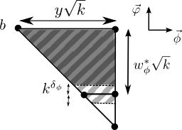
Figure 5. Definition (20) illustrated for $w^{\ast}_{\phi}\leq w^{\ast}_{\varphi}$. We claim that with high probability, in $\mathcal{G}^{k}$, all motorcycles $\bar{a}=(a,\varphi)$ with $a$ in the gray region will cross the line $b+[0,y\sqrt{k}]$, and all such motorcycles with $a$ in the white region will not. We define $\underline{K}(b,y,\varphi)$ to be the number of sites of the PPP in the gray region which spawn motorcycles that travel in direction $\varphi$, and $\overline{K}(b,y,\varphi)$ to be that number for the striped region. The case $w^{\ast}_{\phi}>w^{\ast}_{\varphi}$ is the same figure with $w^{\ast}_{\varphi}\sqrt{k}$ replacing $w^{\ast}_{\phi}\sqrt{k}$.

Lemma 15.

Fix $k\in\mathbb{N}$, a motorcycle $\bar{b}=(b,\phi)$ with $b\in\sqrt{k}\cdot R$, angle $\varphi\in A,\varphi\neq\phi$. For fixed sequences $\underline{y}=\underline{y}(k)=w^{\ast}_{\phi}+o(1)>w^{\ast}_{\phi}$, $\overline{y}=\overline{y}(k)=w^{\ast}_{\phi}-o(1)<w^{\ast}_{\phi}$, as $k\to\infty$,

$$\underline{K}(\bar{b},\underline{y},\varphi,k)\leq K(\bar{b},\underline{y},\varphi,k) b\in\sqrt{k}\cdot R$$ for all w.h.p., (22)

$$K(\bar{b},\overline{y},\varphi,k)\leq\overline{K}(\bar{b},\overline{y},\varphi,k) b\in\sqrt{k}\cdot R$$ for all w.h.p.. (23)

In particular, for $\underline{y}:=w_{\phi}^{\ast}+k^{\delta_{\phi}-1/2}$ and $\overline{y}=w_{\phi}^{\ast}-k^{\delta_{\phi}-1/2}$, then

$$\underline{K}(\bar{b},\underline{y},k)\geq k b\in\sqrt{k}\cdot R$$ for all , w.h.p., (24)

$$\overline{K}(\bar{b},\overline{y},k)\leq k b\in\sqrt{k}\cdot R$$ for all , w.h.p.. (25)

Order the angles in $A$ as $\phi_{1},\ldots,\phi_{M^{\prime}}$ such that the corresponding values $w^{\ast}_{\phi}$ are non-decreasing, that is, if $i<j$, then $w^{\ast}_{i}=w^{\ast}_{\phi_{i}}\leq w^{\ast}_{j}=w^{\ast}_{\phi_{j}}$. We shall prove Lemma 15 by an inductive argument along $i=1,\ldots,|A|$. Each step in the induction involves fixing $i$, and establishing (22) and (23) for pairs $(\phi,\varphi)=(\phi_{i},\phi_{j})$ and $(\phi,\varphi)=(\phi_{j},\phi_{i})$, for all $j=1,\ldots|A|$ such that $j>i$, and then use this and the induction hypothesis to prove (24) and (25) for $\phi=\phi_{i}$. For clarity, we restate each case of Lemma 15 in the induction proof as a lemma in itself.

Lemma 16.

For all $j>1$, Equations (22) and (23) hold for $\phi=\phi_{1}$ and $\varphi=\phi_{j}$.

Proof.

By definition, $w^{\ast}_{\phi}=w^{\ast}_{1}$ and $w^{\ast}_{\varphi}=w^{\ast}_{j}$. As $w^{\ast}_{1}\leq w^{\ast}_{j}$ and $\overline{y}\leq w^{\ast}_{1}$, by the definition of $\overline{K}$ in (21),

$$\overline{K}(\bar{b},\overline{y},\phi_{j},k)=\sum_{Q\subseteq A\backslash\{\phi_{j}\}}\mathcal{P}_{\phi_{j}\cup Q}(\tau_{b}\circ T^{\overline{y}\sqrt{k},\overline{y}\sqrt{k}}_{\phi_{1}\phi_{j}})=\tilde{K}(\bar{b},\overline{y},\phi_{j},k).$$

So $\overline{K}(\bar{b},\overline{y},\phi_{j},k)$ is trivially an upper-bound for $K(\bar{b},\overline{y},\varphi,k)$ by (19). This proves (23).

Now consider the lower bound (22). Since $\underline{y}\geq w^{\ast}_{1}$, by the definition of $\underline{K}$ in (20),

$$\underline{K}(\bar{b},\underline{y},\phi_{j},k)=\sum_{Q\subseteq A\backslash\{\phi_{j}\}}\mathcal{P}_{\phi_{j}\cup Q}(\tau_{b}\circ T^{\underline{y}\sqrt{k},w^{\ast}_{1}\sqrt{k}-k^{\delta_{1}}}_{\phi_{1}\phi_{j}}).$$

For all potential killers $\bar{a}=(a,\varphi)$ of $\bar{b}$ for $\underline{y}$, define $d(\bar{a},\bar{b})$ to be the positive real number such that $d(\bar{a},\bar{b})\sqrt{k}$ is the distance $\bar{a}$ has to travel to meet the path of $\bar{b}$. In order to prove (22), it is enough to show that all potential killers $\bar{a}=(a,\phi_{j})$ with $d(\bar{a},\bar{b})\sqrt{k}<w^{\ast}_{1}\sqrt{k}-k^{\delta_{1}}$ are would-be killers of $\bar{b}$ with high probability. Fix such a motorcycle $\bar{a}$. Until its supposed meeting with $\bar{b}$, $\bar{a}$ can only be killed at most $\tilde{K}(\bar{a},d(\bar{a},\bar{b}),k)$ times. So it is enough to show that

$$\sup_{b\in\sqrt{k}\cdot R}\sup_{a\in\tau_{b}\circ T^{\underline{y}\sqrt{k},w^{\ast}_{1}\sqrt{k}-k^{\delta_{1}}}_{\phi_{1}\phi_{j}}}\tilde{K}(\bar{a},d(\bar{a},\bar{b}),k)\leq k\hskip 10.00002pt\mbox{w.h.p.}$$ (26)

From (18), for all $z>0$,

$$\tilde{K}(\bar{a},z,k)=\sum_{Q\subseteq A\backslash\{\phi_{j}\}}\sum_{\psi\in Q}(\mathcal{P}_{Q}+\mathcal{P}_{Q\cup\phi_{j}})(\tau_{a}\circ T^{\sqrt{k}z,\sqrt{k}z}_{\phi_{j}\psi}).$$ (27)

Set $R_{k}^{\prime}:=\sqrt{k}\cdot R\oplus\tau_{0}\circ T^{\underline{y}\sqrt{k},w_{1}^{\ast}\sqrt{k}-k^{\delta_{1}}}_{\phi_{1}\phi_{j}},$ where $\oplus$ denotes the Minkowski sum. We have

$$\sup_{b\in\sqrt{k}\cdot R}\sup_{a\in\tau_{b}\circ T^{\underline{y}\sqrt{k},w_{1}^{\ast}\sqrt{k}-k^{\delta_{1}}}_{\phi_{1}\phi_{j}}}\tilde{K}(\bar{a},d(\bar{a},\bar{b}),k)$$

$$= \sup_{a\in R_{k}^{\prime}}\sum_{Q\subseteq A\backslash\{\phi_{j}\}}\sum_{\psi\in Q}(\mathcal{P}_{Q}+\mathcal{P}_{Q\cup\phi_{j}})(\tau_{a}\circ T^{d(\bar{a},\bar{b})\sqrt{k},d(\bar{a},\bar{b})\sqrt{k}}_{\phi_{j}\psi})$$ by (27)

$$< \sup_{a\in R_{k}^{\prime}}\sum_{Q\subseteq A\backslash\{\phi_{j}\}}\sum_{\psi\in Q}(\mathcal{P}_{Q}+\mathcal{P}_{Q\cup\phi_{j}})(\tau_{a}\circ T^{w^{\ast}_{1}\sqrt{k}-k^{\delta_{1}},w^{\ast}_{1}\sqrt{k}-k^{\delta_{1}}}_{\phi_{j}\psi}) \mbox{as }d(\bar{a},\bar{b})\sqrt{k}\leq w^{\ast}_{1}\sqrt{k}-k^{\delta_{1}}$$

$$\leq \sum_{Q\subseteq A\backslash\{\phi_{j}\}}\sum_{\psi\in Q}\sup_{a\in R_{k}^{\prime}}(\mathcal{P}_{Q}+\mathcal{P}_{Q\cup\phi_{j}})(\tau_{a}\circ T^{w^{\ast}_{1}\sqrt{k}-k^{\delta_{1}},w^{\ast}_{1}\sqrt{k}-k^{\delta_{1}}}_{\phi_{j}\psi})$$ (28)

Note that

$$\tau_{0}\circ T^{\underline{y}\sqrt{k},w_{1}^{\ast}\sqrt{k}-k^{\delta_{1}}}_{\phi_{1}\phi_{j}}\subset\tau_{0}\circ\sqrt{k}\cdot T^{\underline{y},\underline{y}}_{\phi_{1}\phi_{j}}\subset\tau_{0}\circ T^{2w^{\ast}_{1},2w^{\ast}_{1}}_{\phi_{1}\phi_{j}},$$

so $R_{k}^{\prime}\subset\sqrt{k}\cdot R^{\prime}\subset\mathbb{R}^{2}$ for the compact set $R^{\prime}:=R\oplus\tau_{0}\circ T^{2w^{\ast}_{1},2w^{\ast}_{1}}_{\phi_{1}\phi_{j}}\subset\mathbb{R}^{2}$, independent of $k$. Thus (28) is upper bounded by

$$\sum_{Q\subseteq A\backslash\{\phi_{j}\}}\sum_{\psi\in Q}\sup_{a\in\sqrt{k}\cdot R^{\prime}}(\mathcal{P}_{Q}+\mathcal{P}_{Q\cup\phi_{j}})(\tau_{a}\circ T^{w^{\ast}_{1}\sqrt{k}-k^{\delta_{1}},w^{\ast}_{1}\sqrt{k}-k^{\delta_{1}}}_{\phi_{j}\psi}).$$ (29)

As the compact set $R^{\prime}$ is independent of $k$, one can apply Lemma 13 to (29). Union bound over the summands tells us that the sum in (29) is not far from the mean, which is

$$\sum_{Q\subseteq A\backslash\{\phi_{j}\}}\sum_{\psi\in Q}\mathbb{E}(\mathcal{P}_{Q}+\mathcal{P}_{Q\cup\phi_{j}})(\tau_{a}\circ T^{w^{\ast}_{1}\sqrt{k}-k^{\delta_{1}},w^{\ast}_{1}\sqrt{k}-k^{\delta_{1}}}_{\phi_{j}\psi})=(w^{\ast}_{1}\sqrt{k}-k^{\delta_{1}})^{2}\mathcal{E}(\mathbf{1},\phi_{j}).$$

Explicitly, for each $Q\subseteq A\backslash\{\phi_{j}\}$, and each $\psi\in Q$, apply Lemma 13 with the sets $R=R^{\prime}$, $S=T^{w^{\ast}_{1}-k^{\delta_{1}-1/2},w^{\ast}_{1}-k^{\delta_{1}-1/2}}_{\phi_{j}\psi}$ and the Poisson point processes $k\cdot\mathcal{P}_{Q}$ and $k\cdot\mathcal{P}_{Q\cup\phi_{j}}$ to obtain

$$\sup_{a\in R^{\prime}}(\mathcal{P}_{Q}+\mathcal{P}_{Q\cap\phi_{j}})(\tau_{b}\circ T^{w^{\ast}_{1}\sqrt{k}-k^{\delta_{1}},w^{\ast}_{1}\sqrt{k}-k^{\delta_{1}}}_{\phi_{j}\psi})\leq k(\mu_{Q}+\mu_{Q\cap\phi_{j}})|S|+O(|S|k^{1/2+\epsilon})\mbox{ w.h.p.}$$

Note that $|S|=O((w^{\ast}_{1}-k^{{\delta_{1}}-1/2})^{2})\leq O((w^{\ast}_{1})^{2})=O(1),$ so $O(|S|k^{1/2+\epsilon})=O(k^{1/2+\epsilon})$. Fix $0<\epsilon<\delta_{\phi}$. Taking a union bound over all pairs $(Q,\psi)$, we get

$$\sum_{Q\subseteq A\backslash\{\phi_{j}\}}\sum_{\psi\in Q}\sup_{a\in\sqrt{k}\cdot R^{\prime}}(\mathcal{P}_{Q}+\mathcal{P}_{Q\cup\phi_{j}})(\tau_{a}\circ T^{w^{\ast}_{1}\sqrt{k}-k^{\delta_{1}},w^{\ast}_{1}\sqrt{k}-k^{\delta_{1}}}_{\phi_{j}\psi})=(w^{\ast}_{1}\sqrt{k}-k^{\delta_{1}})^{2}\mathcal{E}(\mathbf{1},\phi_{j})+O(k^{1/2+\epsilon}).$$

Finally, by (5), for some constant $C>0$, with high probability

$$(w^{\ast}_{1}\sqrt{k}-k^{\delta_{1}})^{2}\mathcal{E}(\mathbf{1},\phi_{j})+O(k^{1/2+\epsilon})\leq\left(\frac{w^{\ast}_{1}\sqrt{k}-k^{\delta_{1}}}{w^{\ast}_{1}}\right)^{2}+O(k^{1/2+\epsilon})\leq k-Ck^{1/2+{\delta_{1}}}\leq k,$$

for $k$ large enough. This establishes (22) for the case $\phi=\phi_{1}$, $\varphi=\phi_{j}$, $j>1$. $\Box$

Lemma 17.

Equations (24) and (25) hold for $\phi=\phi_{1}$.

Proof.

Define the weight vector $w=\bar{y}\sqrt{k}\cdot\mathbf{1}$. For each $Q\subseteq A\backslash\{\phi_{1}\}$, set $S=T^{w}_{\phi_{1}Q}$, and for each $\phi_{j}\in Q$, apply Lemma 13 with sets $R,S$, and the Poisson point process $\mathcal{P}_{\phi_{1}\phi_{j}}$. As before, note that in each case $S$, $|S|=O(1)$. By the union bound over all such sets $Q$ and such angles $\phi_{j}$,

$$\sup_{b\in\sqrt{k}\cdot R}\overline{K}(\bar{b},\overline{y},k) \leq\sum_{Q\subseteq A\backslash\{\phi_{1}\}}\sum_{\varphi\in Q}\sup_{b\in\sqrt{k}\cdot R}|(\mathcal{P}_{Q}+\mathcal{P}_{Q\cup\phi_{1}})\cap(\tau_{b}\circ T^{w}_{\phi_{1}Q})|$$ by (23)

$$\leq\mathcal{E}(w,\phi_{1})+O(|S|k^{1/2+\epsilon})$$ by Lemma 13

$$=\left(\frac{w_{1}^{\ast}\sqrt{k}-k^{\delta_{\phi_{1}}}}{w_{1}^{\ast}}\right)^{2}+O(k^{1/2+\epsilon}) \mbox{ by definition of }\bar{y}$$

$$\leq k-Ck^{1/2+{\delta_{\phi_{1}}}}\leq k$$ (30)

with high probability, for large enough $k$, and for some constant $C>0$. This proves (25) for $\phi=\phi_{1}$.

Similarly, define the weight vector $w$ with

$$w_{1}=\underline{y}=w^{\ast}_{1}+k^{\delta_{1}-1/2},\hskip 10.00002ptw_{j}=w^{\ast}_{1}-k^{\delta_{1}-1/2}\mbox{ for }j>1.$$

By the same argument as above, from (22) for $\phi=\phi_{1}$ and Lemma 13, we have

$$\inf_{b\in\sqrt{k}\cdot R}\underline{K}(\bar{b},\underline{y},k)\geq\mathcal{E}(\sqrt{k}\cdot w,\phi_{1})+O(k^{1/2+\epsilon}).$$

By the definition of $\mathcal{E}(\sqrt{k}\cdot w,\phi_{1})$ given in (1), and the geometry of the regions $T^{\sqrt{k}\cdot w}_{\phi Q}$, we have

$$\mathcal{E}(\sqrt{k}\cdot w,\phi_{1})=\mathcal{E}((w^{\ast}_{1}\sqrt{k}+k^{\delta_{1}})\cdot\mathbf{1},1)-O(k^{2\delta_{1}}).$$

Therefore, for some constant $C>0$,

$$\inf_{b\in\sqrt{k}\cdot R}\underline{K}(\bar{b},\underline{y},k)\geq\left(\frac{w_{1}^{\ast}\sqrt{k}+k^{\delta_{1}}}{w_{1}^{\ast}}\right)^{2}-O(k^{2\delta_{1}})+O(k^{1/2+\epsilon})=k+Ck^{1/2+\delta_{1}}\geq k$$

with high probability for large enough $k$. This proves (24) for $\phi=\phi_{1}$. $\Box$

Lemma 18.

For all $j>1$, Equations (22) and (23) hold for $\varphi=\phi_{1}$, $\phi=\phi_{j}$.

Proof.

If $w^{\ast}_{\phi}=w^{\ast}_{j}=w^{\ast}_{\varphi}=w^{\ast}_{1}$, then the previous argument applies. So we only need to consider $\phi=\phi_{j}$ such that $w^{\ast}_{j}>w^{\ast}_{1}$. In this case, for large enough $k$,

$$\underline{K}(\bar{b},\underline{y},\phi_{1},k)=\sum_{Q\subseteq A\backslash\{\phi_{1}\}}|\mathcal{P}_{\phi_{1}\cup Q}\cap(\tau_{b}\circ T^{\underline{y}\sqrt{k},w^{\ast}_{1}\sqrt{k}-k^{\delta_{1}}}_{\phi_{j}\phi_{1}})|$$

and

$$\overline{K}(\bar{b},\overline{y},\phi_{1},k)=\sum_{Q\subseteq A\backslash\{\phi_{1}\}}|\mathcal{P}_{\phi_{1}\cup Q}\cap(\tau_{b}\circ T^{\overline{y}\sqrt{k},w^{\ast}_{1}\sqrt{k}+k^{\delta_{1}}}_{\phi_{j}\phi_{1}})|,$$

where here $\overline{y}=w^{*}_{j}-o(1)$ and $\underline{y}=w^{*}_{j}+o(1)$. For the lower bound, we need to show that potential killers $\bar{a}=(a,\phi_{1})$ with $d(\bar{a},\bar{b})\sqrt{k}<w^{\ast}_{1}\sqrt{k}-k^{\delta_{1}}$ are would-be killers. Let $R^{\prime}:=R\oplus\tau_{0}\circ T^{\overline{y},w^{\ast}_{1}-k^{\delta_{1}-1/2}}_{\phi_{j}\phi_{1}}$. By (23) and (25) for the case $\bar{a}=(a,\phi_{1})$ proved in Lemmas 16 and 17, we have

$$\sup_{b\in\sqrt{k}\cdot R}\sup_{a\in\tau_{b}\circ T^{\overline{y}\sqrt{k},w^{\ast}_{1}\sqrt{k}-k^{\delta_{1}}}_{\phi_{j}\phi_{1}}}K(\bar{a},d(\bar{a},\bar{b}),k)\leq\sup_{a\in\sqrt{k}\cdot R^{\prime}}\overline{K}(\bar{a},w^{\ast}_{1}-k^{{\delta_{1}}-1/2},k)\leq k,$$

so this is the desired result. Similarly, for the upper bound, we need to show that potential killers with $d(\bar{a},\bar{b})\sqrt{k}>w^{\ast}_{1}\sqrt{k}+k^{\delta_{1}}$ cannot meet $\bar{b}$ in $\mathcal{G}^{k}$. Apply (22) and (24) for the case $\bar{a}=(a,\phi_{1})$ proved in Lemmas 16 and 17, we have

$$\inf_{b\in\sqrt{k}\cdot R}\inf_{a\in\tau_{b}\circ\left(T^{\underline{y}\sqrt{k},\underline{y}\sqrt{k}}_{\phi_{j}\phi_{1}}\backslash T^{\underline{y}\sqrt{k},w^{\ast}_{1}\sqrt{k}+k^{\delta_{1}}}_{\phi_{j}\phi_{1}}\right)}K(\bar{a},d(\bar{a},\bar{b}),k)\geq\inf_{a\in\sqrt{k}\cdot R^{\prime}}\underline{K}(\bar{a},w^{\ast}_{1}+k^{{\delta_{1}}-1/2},k)\geq k\hskip 10.00002pt\mbox{w.h.p.},$$

where $R^{\prime}=R+\tau_{0}\circ\left(T^{\underline{y},\underline{y}}_{\phi_{j}\phi_{1}}\backslash T^{\underline{y},w^{\ast}_{1}\sqrt{k}+k^{\delta_{1}}}_{\phi_{j}\phi_{1}}\right)$. This completes the proof. $\Box$

Suppose Lemma 15 holds for all $\phi_{1},\ldots,\phi_{i-1}$. This means we have proven that (24) and (25) hold for $\bar{b}=(b,\phi_{\ell})$ for all $\ell=1,\ldots,i-1$, and that (22) and (23) hold for pairs $(\phi,\varphi)=(\phi_{\ell},\phi_{j})$ and $(\phi,\varphi)=(\phi_{j},\phi_{\ell})$, for all $\ell=1,\ldots,i-1$, and $j>\ell$. Thus, we may assume that $w_{i-1}^{\ast}<w_{i}^{\ast}$. Lemmas 16, 17 and 18 establish the base case with $\phi=\phi_{1}$. We now prove the various induction statements for $\phi=\phi_{i}$.

Lemma 19.

Equations (22) and (23) hold for $\phi=\phi_{i}$, $\varphi=\phi_{j}$, $j\neq i$.

Proof.

The induction hypothesis already covers the case $j<i$. Consider the case $j>i$. Again, the upper bound is equal to $\tilde{K}(\bar{b},y,\phi_{j},k)$, so we only need to establish the lower bound. From the induction assumptions, by the same consideration as in Lemma 16, it is enough to show that

$$\sup_{b\in\sqrt{k}\cdot R}\sup_{a\in\tau_{b}\circ T^{y\sqrt{k},,w^{\ast}_{\phi_{i}}\sqrt{k}-k^{\delta_{\phi_{i}}}}_{\phi_{i}\phi_{j}}}\tilde{K}^{i,j}(\bar{a},d(\bar{a},\bar{b}),k)\leq k\hskip 10.00002ptw.h.p.,$$ (31)

where

$$\tilde{K}^{i,j}(\bar{a},z,k):=\sum_{\ell=1}^{i-1}\overline{K}(\bar{a},z,\phi_{\ell},k)+\sum_{\ell=i,\ell\neq j}^{|A|}\tilde{K}(\bar{a},z,\phi_{\ell},k).$$ (32)

With $R^{\prime}$ defined analogous to the base case, we have

$$\sup_{b\in\sqrt{k}\cdot R}\sup_{a\in\tau_{b}\circ T^{y\sqrt{k},w^{\ast}_{\phi_{i}}\sqrt{k}-k^{\delta_{\phi_{i}}}}_{\phi_{i}\phi_{j}}}\tilde{K}^{i,j}(\bar{a},d(\bar{a},\bar{b}),k)\leq\sup_{a\in\sqrt{k}\cdot R^{\prime}}\tilde{K}^{i,j}(\bar{a},w^{\ast}_{\phi_{i}}-k^{\delta_{\phi_{i}}-1/2},k)$$

$$\leq\sup_{a\in\sqrt{k}\cdot R^{\prime}}\sum_{\ell=1}^{i-1}\overline{K}(\bar{a},w^{\ast}_{\phi_{i}}-k^{\delta_{\phi_{i}}-1/2},\phi_{\ell},k)+\sup_{a\in\sqrt{k}\cdot R^{\prime}}\sum_{\ell=i,\ell\neq j}^{|A|}\tilde{K}(\bar{a},w^{\ast}_{\phi_{i}}-k^{\delta_{\phi_{i}}-1/2},\phi_{\ell},k)$$

$$\leq\sum_{\ell=1}^{i-1}\sum_{Q\subseteq A\backslash\{\phi_{\ell}\}}\mathbb{E}\mathcal{P}_{\phi_{\ell}\cup Q}(\tau_{a}\circ T^{w^{\ast}_{\phi_{i}}\sqrt{k}-k^{\delta_{\phi_{i}}},w^{\ast}_{\phi_{\ell}}\sqrt{k}+k^{\delta_{\phi_{\ell}}}}_{\phi_{j}\phi_{\ell}})$$

$$+\sum_{\ell=i,\ell\neq j}^{|A|}\sum_{Q\subseteq A\backslash\{\phi_{\ell}\}}\mathbb{E}\mathcal{P}_{\phi_{\ell}\cup Q}(\tau_{a}\circ T^{w^{\ast}_{\phi_{i}}\sqrt{k}-k^{\delta_{\phi_{i}}},w^{\ast}_{\phi_{i}}\sqrt{k}-k^{\delta_{\phi_{i}}}}_{\phi_{j}\phi_{\ell}})+O(k^{1/2+\epsilon})\hskip 30.00005pt\mbox{ by Lemma \ref{lem:sup.bound}},$$

where $\epsilon>0$ is an arbitrarily small constant. Define the weight vector $w\in\mathbb{R}^{M}$ with

$$w_{\ell}=w^{\ast}_{\ell}+k^{\delta_{\ell}-1/2}\mbox{ for }\ell=1,\ldots,i-1,\hskip 10.00002ptw_{\ell}=w^{\ast}_{i}-k^{\delta_{i}-1/2}\mbox{ for }\ell\geq i.$$

Then the sum of the expectations in the last expression is equal to $\mathcal{E}(\sqrt{k}\cdot w,\phi_{j})$. Define $w^{\prime}\in\mathbb{R}^{M}$ via

$$w^{\prime}_{\ell}=w^{\ast}_{\ell},\mbox{ for }\ell=1,\ldots,i-1,\hskip 10.00002ptw^{\prime}_{\ell}=w^{\ast}_{i},\mbox{ for }\ell\geq i.$$

By Lemma 14, we have

$$\mathcal{E}(\sqrt{k}\cdot w,\phi_{j})=\mathcal{E}(\sqrt{k}\cdot w^{\prime},\phi_{j})+o(k^{1/2+\delta_{i}})-Ck^{1/2+\delta_{i}}$$

for some constant $C>0$. Now, by definition of $w^{\ast}$,

$$\mathcal{E}(\sqrt{k}\cdot w^{\prime},\phi_{j})=k.$$

Therefore, the quantity we need is upper-bounded by

$$k+o(k^{1/2+\delta_{i}})-Ck^{1/2+\delta_{i}}+O(k^{1/2+\epsilon})=k-Ck^{1/2+\delta_{\phi_{i}}}\leq k$$

with high probability for large enough $k$. This proves (31), as needed. $\Box$

Lemma 20.

Equations (24) and (25) hold for $\phi=\phi_{i}$.

Proof.

Define the weight vector $w\in\mathbb{R}^{M}$ by

$$w_{\ell}=w_{\ell}^{\ast}+k^{\delta_{\ell}-1/2}\mbox{ if }\ell\leq i,\qquad w_{\ell}=\bar{y}=w_{i}^{\ast}-k^{\delta_{i}-1/2}\mbox{ if }\ell>i.$$

By the same argument as in Lemma 17, with high probability,

$$\sup_{b\in\sqrt{k}\cdot R}\overline{K}(\bar{b},\overline{y},k) \leq\sum_{Q\subseteq A\backslash\{\phi_{i}\}}\sum_{\varphi\in Q}\sup_{b\in\sqrt{k}\cdot R}(\mathcal{P}_{Q}+\mathcal{P}_{Q\cup\phi_{i}})(\tau_{b}\circ T^{\sqrt{k}\cdot w}_{\phi_{i}Q}) \phi=\phi_{i}$$ by (23) for

$$\leq\mathcal{E}(\sqrt{k}\cdot w,\phi)+O(k^{1/2+\epsilon}) \mbox{ by Lemma \ref{lem:sup.bound}}.$$ (33)

By the induction hypothesis, we have $\delta_{i}>\delta_{\ell}$ for $\ell<i$, $w_{i}^{\ast}>w_{i-1}^{\ast}$. By Lemma 14, we have

$$\mathcal{E}(\sqrt{k}\cdot w,\phi_{i})=k+o(k^{1/2+\delta_{i}})-Ck^{1/2+\delta_{i}}$$

for some constant $C>0$. As $\epsilon>0$ in (33) is an arbitrary constant,

$$\sup_{b\in\sqrt{k}\cdot R}\overline{K}(\bar{b},\overline{y},k)\leq k+o(k^{1/2+\delta_{i}})+O(k^{1/2+\epsilon})-Ck^{1/2+\delta_{i}}\leq k-\frac{C}{2}k^{1/2+\delta_{i}}\leq k$$

with high probability, large enough $k$. This proves (25) for $\phi=\phi_{i}$.

Similarly, define the weight vector $w\in\mathbb{R}^{M}$ with

$$w_{\ell}=w^{\ast}_{\ell}-k^{\delta_{\ell}-1/2}\mbox{ if }\ell<i,\hskip 10.00002ptw_{\ell}=w^{\ast}_{i}+k^{\delta_{i}-1/2}\mbox{ if }\ell\geq i.$$

By the same argument as above, with (22) for $\phi=\phi_{i}$ and Lemma 13, we have

$$\inf_{b\in\sqrt{k}\cdot R}\underline{K}(\bar{b},\underline{y})\geq\mathcal{E}(\sqrt{k}\cdot w,\phi_{i})+O(k^{1/2+\epsilon}).$$

By Lemma 14,

$$\mathcal{E}(\sqrt{k}\cdot w,\phi_{i})=k-o(k^{1/2+\delta_{i}})+Ck^{1/2+\delta_{i}}$$

for some constant $C>0$. As $\epsilon>0$ is an arbitrarily small constant,

$$\inf_{b\in\sqrt{k}\cdot R}\underline{K}(\bar{b},\underline{y})\geq k+Ck^{1/2+\delta_{i}}-o(k^{1/2+\delta_{i}})+O(k^{1/2+\epsilon})\geq k+\frac{C}{2}k^{1/2+\delta_{i}}\geq k$$

with high probability. This proves (24) for $\phi=\phi_{i}$. $\Box$

Lemma 21.

Equations (22) and (23) hold for $\varphi=\phi_{i}$, $\phi=\phi_{j}$, $j>i$.

Proof.

The proof is identical to that of Lemma 18. $\Box$

Proof of Proposition 11.

By (24) and (25)

$$\overline{y}\sqrt{k}=w^{\ast}_{\phi}\sqrt{k}-k^{\delta_{\phi}}\leq\sup_{b\in\sqrt{k}\cdot R}L^{k}((b,\phi))\leq\underline{y}=w^{\ast}_{\phi}\sqrt{k}+k^{\delta_{\phi}}\hskip 10.00002pt\mbox{ w.h.p.}$$

Rearranging gives

$$\sup_{b\in\sqrt{k}\cdot R}|\frac{L^{k}((b,\phi))}{\sqrt{k}}-w^{\ast}_{\phi}|\leq k^{\delta_{\phi}-1/2}=o(1),$$

as desired. $\Box$

Example 22.

Suppose $\mathcal{G}^{1}$ is the rectangular Gilbert tessellation studied in [3]. That is, each site of $\mathcal{P}$, there are four motorcycles that travel in directions the four directions north, south, east, west. Let $\mathcal{G}^{k}$ be the iterated Gilbert model. Then Theorem 10 states that $\mathcal{G}^{k}(\frac{1}{k})$ converges to the classical Poisson line process $\mathcal{G}^{\infty}$ with cylindrical measure $2\lambda\times(\delta_{-}\delta_{|})$, where $\delta_{-}$ and $\delta_{|}$ are the Dirac delta measures at the points $0$ and $\pi/2$ on the unit circle, respectively.

3.2. Iterated Gilbert with initial complex

We can generalize the iterated Gilbert model by replacing the initial sites $\mathcal{P}$ by a germ-and-grain model, where at each site in $\mathcal{P}$, one attaches an i.i.d. random polyhedral complex, which contains vertices at which the motorcycles start. Let $\mathcal{G}^{0}$ be the union of these initial polyhedral complexes, called the initial complex.

The general iterated Gilbert model $\mathcal{G}^{k}$ starting with $\mathcal{G}^{0}$ features, for each initial polyhedral complex, a collection of motorcycles starting at some points of the complex. It is assumed that, for each given polyhedral complex, an arm starting from this complex never crosses the complex in questions again, nor any other different arm of the polyhedral complex in question. Each such motorcycle starts with a capital of $k$ lives and looses one live when it crosses either another body of $\mathcal{G}^{0}$ or the path of a motorcycle emanating from another body of $\mathcal{G}^{0}$. For a compact set $V\subset\mathbb{R}^{2}$, define its radius to be the radius of the smallest ball containing $V$. If the radius of the polyhedral complex at each site is at most $r>0$ for some constant $r$, and has finitely many facets, edges and vertices, then one can show that for each $k=1,2,\ldots$, the general iterated Gilbert model $\mathcal{G}^{k}$ starting with $\mathcal{G}^{0}$ is still a random mosaic with finite intensity.

Note that in the presence of initial complexes, the situation where one multiplies the intensity of $\mathcal{P}$ by $\frac{1}{k}$ and that where one rescales space by $\sqrt{k}$ do not coincide anymore. In the former case, initial complexes are not scaled, whereas they are in the latter case. In what follows, we consider the former interpretation, namely that of a Poisson point process of centroids with intensity $\frac{\lambda}{k}$ and no rescaling of the initial complexes.

We claim that $\mathcal{G}^{0}$ does not affect the scaling limit. In particular, if the induced angle distributions on the motorcycles satisfy the hypotheses of Theorem 10, then Theorem 10 holds unchanged. To see this, first, note that as $k\to\infty$, for a compact set $W\subset\mathbb{R}^{2}$, $\mathcal{G}^{0}(\frac{1}{k})\cap W\to\emptyset$. Thus, points in $\mathcal{G}^{0}$ do not appear in the limit. Second, we claim that $\mathcal{G}^{0}$ does not affect the argument leading to Theorem 10 regarding the distance a motorcycle can travel with $k$ lives. Indeed, fix a motorcycle $\bar{b}=(b,\phi)$, and consider its number of would-be killers on $b+[0,y\sqrt{k}\cdot\overrightarrow{\phi}]$. On this interval, $\bar{b}$ can now hit lines in $\mathcal{G}^{0}$ and lose more lives. But such lines must come from polyhedral complexes whose centroids are within Euclidean distance $r$ of the line. The number of such centroid is Poisson with mean $O(\sqrt{k})$, with fluctuations of order $O(k^{1/4+\epsilon^{\prime}})$. This is well-below the fluctuations $O(k^{1/2+\epsilon})$ of the number of would-be killers of $\bar{b}$, and thus our argument for Theorem 10 essentially goes through unchanged.

Theorem 23.

Let $\mathcal{G}^{k}(\mathcal{P},\mathcal{A})$ be an iterated Gilbert mosaic with initial complex $\mathcal{G}^{0}$, whose polyhedral complex at each site of $\mathcal{P}$ has radius at most $r>0$. Then Theorem 10 applies. That is, as $k\to\infty$, for any compact window $W\subset\mathbb{R}^{2}$,

$$\mathcal{G}^{k}\left(\frac{1}{k}\right)\cap W\to\mathcal{G}^{\infty}\cap W\mbox{ in probability},$$

where $\mathcal{G}^{\infty}$ is a Poisson line process with cylindrical measure $\Lambda dr\times\Theta(d\theta)$, with

$$\Lambda=\sum_{\phi\in A}w^{*}_{\phi}\sum_{Q\subset A,\phi\in Q}\mu_{Q}$$

and $\Theta$ the probability measure with mass

$$\frac{1}{\Lambda}w^{*}_{\phi}\sum_{Q\subset A,\phi\in Q}\mu_{Q}$$

at $\phi^{\perp}$, for all $\phi\in A$, where $w^{\ast}$ is defined by (4).

4. Application: Poisson tropical plane curves

This section provides some background on tropical geometry, and discusses why the iterated Gilbert model is the right way to study a process of tropical plane curves from the view point of stochastic geometry.

4.1. Tropical polynomials

Consider the tropical min-plus algebra $(\bar{\mathbb{R}},\odot,\oplus)$, where $\bar{\mathbb{R}}=\mathbb{R}\cup\{+\infty\}$, $a\odot b=a+b$, $a\oplus b=\min(a,b)$. A tropical polynomial $f$ in two variables has the form

$$f(x,y)=\bigoplus_{i,j\in\mathbb{N}}c_{ij}\odot x^{\odot i}y^{\odot j}=\min_{i,j\in\mathbb{N}}(c_{ij}+ix+jy),$$ (34)

where the coefficients $c_{ij}\in\bar{\mathbb{R}}$. It is assumed that only finitely many $c_{ij}$’s are finite (recall that $+\infty$ is the zero of $\oplus$, so that this condition simply says that there are only finitely many non zero-monomials). As in classical algebra, the support of $f$ is

$$\text{supp}(f)=\{(i,j)\in\mathbb{N}^{2}:c_{ij}<\infty\}.$$

The convex hull of the support of $f$ is the Newton polygon of $f$. For each $c_{ij}<\infty$, the graph of each term $(x,y)\mapsto c_{ij}\odot x^{\odot i}y^{\odot j}$ is a plane in $\mathbb{R}^{3}$. Thus, the graph of $f$ is the minimum of finitely many planes, and is piecewise affine, see Figure 6. The tropical zeros, or tropical variety of $f$, denoted by $V_{f}$, is the set of points $(x,y)\in\mathbb{R}^{2}$ where the minimum in (34) is achieved at least twice, or in other words, points where $f$ is non-differentiable. This definition of zeros allows many classical theorems in algebra to carry over in the tropical setting. For example, the Fundamental Theorem of Algebra [15, §1] applies tropically, meaning that the tropical polynomials can be factorized into a product of affine terms based on its zeros. A deeper result is the Fundamental Theorem of Tropical Algebraic Geometry [15, §3], which gives a correspondence between the zeros of tropical polynomials and those of classical polynomials when the former are obtained through tropicalization of the latter over non-Archimedian fields.

For $d\in\mathbb{N}$, $0<d<\infty$, say that $f$ is standard with degree $d$ if its Newton polygon is the triangle with vertices $(0,0)$, $(0,d)$ and $(d,0)$. In this case, we say that $V_{f}$ is a standard tropical plane curve. Since the rest of the text is about such curves, for simplicity we will refer to them as tropical curves. The restriction to standard Newton polygons is fundamental to the results in this section, since it ensures that the unbounded segments (arms) of the tropical curve can only take on certain angles.

4.1.1. Tropical plane curves and duality

A tropical plane curve $V_{f}$ is a polyhedral complex. It is convenient to work with the dual of this complex. This is the regular subdivision of the negative of the Newton polygon of $f$ with lift given by the coefficients $c_{ij}$’s. This fact holds for tropical hypersurfaces of arbitrary dimensions [15, Proposition 3.1.6]. For simplicity we only state the definitions for the case of plane curves.

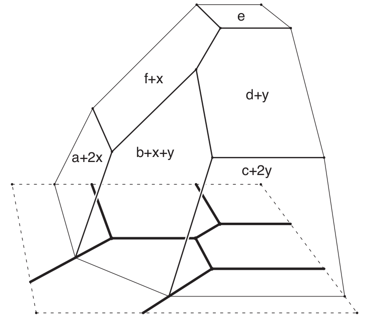
Figure 6. The graph and the tropical plane curve of degree $2$ defined by $f(x,y)=a\odot x^{\odot 2}\oplus b\odot x\odot y\oplus c\odot y^{\odot 2}\oplus d\odot y\oplus e\oplus f\odot x$. Figure taken from [15, Figure 1.3.2]. The graph is the three-dimensional structure. The tropical curve is the projection of the non-differentiable points of this three-dimensional structure on the plane.

We now define this regular subdivision, which is illustrated in Figure 7. For each integer point $(i,j)$ of the Newton polygon, one ‘lifts’ it up to height $c_{ij}$; one then takes the convex hull of the points $(i,j,c_{ij})\in\mathbb{R}^{3}$, reflects the figure about the origin in the $(i,j)$ plane, and finally projects the lower faces of this convex hull back down to the plane. This is the regular subdivision aforementioned.

To see its connection with $V_{f}$, define $g:=-f$, let $\hat{g}:\mathbb{R}^{2}\to\mathbb{R}$ be its Legendre transform

$$\hat{g}(u,v)=\sup_{(x,y)\in\mathbb{R}^{2}}(ux+vy-g(x,y)).$$

By a direct calculation, one finds that the graph of $\hat{g}$ is the lower convex hull of the set of points $\{(-(i,j),c_{ij}):(i,j)\in\text{supp}(f)\}\subset\mathbb{R}^{3}$. Its projection onto $\mathbb{R}^{2}$ hence forms the regular subdivision of $-\text{Newt}(f)$ with lift $c_{ij}$’s. By duality of the Legendre transform, one gets that $\hat{\hat{g}}=g$. By a definition chase, one finds that this implies that the polyhedral complex dual to the regular subdivision is precisely the tropical plane curve defined by $f$. Figure 8 gives a second illustration of this duality.

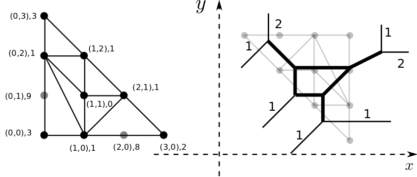
Figure 7. Here $f(x,y)=3\odot y^{\odot 3}\oplus 1\odot y^{\odot 2}\oplus 1\odot x\odot y^{\odot 2}\oplus 9\odot y\oplus x\odot y\oplus 1\odot x^{\odot 2}\odot y\oplus 3\oplus 1\odot x\oplus 8\odot x^{\odot 2}\oplus 2\odot x^{\odot 3},$ a standard tropical curve of degree $3$. Left: the Newton polygon $\text{Newt}(f)$ with the lift $c_{ij}$’s. The two lattice points $(0,1)$ and $(2,0)$ are not vertices of the lower convex hull of the lifted points, and hence not vertices of the regular subdivision. These two points are shown in gray. Right: the tropical plane curve with $-\text{Newt}(f)$ shown in gray. The body of the curve is shown in bold. The arms are shown in black, with numbers indicating their multiplicities.

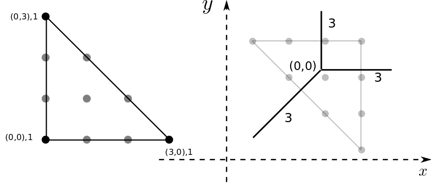
Figure 8. The Newton polygon (left) and the tropical plane curve (right) defined by the polynomial $f_{1}(x,y)=x^{\odot 3}\oplus y^{\odot 3}\oplus 0$. As a set, this curve equals the tropical line given by $f_{2}(x,y)=x\oplus y\oplus 0$. However, each arm of this curve has multiplicity $3$, while each arm of the tropical line only has multiplicity $1$.

Unlike in classical algebra, even up to trivial scaling of coefficients, a tropical polynomial is not uniquely determined by its set of zeros, or equivalently by its plane curve. Here is however an observation that will be used later. Let $g$ be a tropical polynomial with $ij$-th coefficient equal to $c_{ij}(g)$. Let $x^{*}$ and $y^{*}$ be real numbers. Let $f$ be the tropical polynomial with $ij$-th coefficient defined by

$$c_{ij}(f)=\left\{\begin{array}[]{ccc}c_{ij}(g)+ix^{*}+jy^{*}&\mbox{ if }&c_{ij}(g)<\infty\\ \infty&\mbox{ if }&c_{ij}(g)=\infty.\end{array}\right.$$

Any zero $(x,y)$ of $g$ can be mapped in a bijective way to a zero $(\widetilde{x},\widetilde{y})$ of $f$ through the tropical linear transformation $(x,y)=(x^{*}\odot\widetilde{x},y^{*}\odot\widetilde{y})$. Hence, the zeros of $g$ are tropically scaled versions of those of $f$, with the scaling coefficients determined by $(x^{*},y^{*})$.

4.1.2. Tropical plane curves as sets

Let $f$ be a standard tropical polynomial with finite degree $d$. Its corresponding tropical curve $V_{f}$ is a closed set, or more precisely, a polyhedral complex in $\mathbb{R}^{2}$. It is the union of unbounded half-lines called arms, denoted by $a(V_{f})$, and a connected of set of line segments. We call the union of the later set of line segments the body, denoted by $b(V_{f})$. Vertices, half-lines and line segments of $V_{f}$ are collectively called its polyhedral facets. The multiplicity $m(\sigma)$ of an arm or line segment $\sigma$ of $V_{f}$ is the lattice length of the edge of the regular subdivision of the Newton polygon of $f$ that is dual to $\sigma$. If $p\in\mathbb{R}^{2}$ is a common zero of the polynomials $f_{1}$ and $f_{2}$, formed by the intersection of polyhedral facets $\sigma_{1}\subset V_{f_{1}}$ and $\sigma_{2}\subset V_{f_{2}}$, then the multiplicity of $p$ is $m(p)=m(\sigma_{1})m(\sigma_{2})$. See [15, §3] for further details.

Say that an arm is horizontal (resp. vertical and diagonal) if it is parallel to the $(0,1)$ (resp. $(0,1)$ and $(1,1)$) direction, respectively. An important property of standard tropical plane curves of degree $d$ is that they have precisely $d$ arms of each of these three types. This is not necessarily true for non-standard tropical plane curves.

Lemma 24.

Let $V_{f}$ be a tropical curve of degree $d$. Then an arm of $V_{f}$ can only have slope parallel to the $(0,1),(1,0)$ or $(1,1)$ direction. Furthermore, counting multiplicities, $V_{f}$ has precisely $d$ arms of each type.

Proof.

Let $\sigma$ be an arm or line segment of $V_{f}$. Then $\sigma$ is an arm of $V_{f}$ if and only if it is dual to an edge on the boundary of the Newton polygon of $V_{f}$ in its regular subdivision. Thus, an arm of $V_{f}$ can only have slope perpendicular to the slopes of the boundary edges of the Newton polygon of $V_{f}$, which are $(0,1),(1,0)$ and $(1,-1)$. This proves the first statement. For the second, note that the total multiplicities of all horizontal arms equals the lattice length of the line segment $[(0,0),(0,d)]$, which is $d$. Thus, counting multiplicities, $V_{f}$ has $d$ horizontal arms. The vertical and diagonal cases are proven similarly. $\Box$

Definition 25 (Centroid function).

Let $\mathcal{C}$ be the set of compact sets in $\mathbb{R}^{2}$. A centroid function $c:\mathcal{C}\to\mathbb{R}^{2}$ is a measurable function such that

$$c(C+y)=y+c(C),\hskip 10.00002pty\in\mathbb{R}^{2},C\in\mathcal{C},$$

where $C+y$ is the translated set $\{x+y:x\in C\}$.

Examples of centroid functions include the center of mass of the set, or its left-most point. Since the body of a tropical curve is compact, we define the centroid of a tropical curve to be the centroid of its body. By Lemma 24, an arm of a tropical curve can therefore be represented as a mark $(a,\phi)\in\mathbb{R}^{2}\times\{0,\pi/2,5\pi/4\}$, where $\phi$ is the angle of its ray with respect to the $(1,0)$ vector, and $a$ is the coordinates of its apex with respect to the centroid of the curve. We can thus identify $V_{f}$ as a pair $(b(V_{f}),a(V_{f}))$, consisting of a compact set $b(V_{f})$, its body, and a set of marks $a(V_{f})$, representing its arms. Let $\mathcal{V}\subset\mathcal{C}\times\mathbb{R}^{2}\times\{0,\pi/2,5\pi/4\}$ denote the set of all such pairs of compact sets and marks which represent some tropical curve $f$.

4.2. A Poisson class of tropical polynomials in two variables

The aim of this subsection is to introduce the Poisson based ensemble of random tropical polynomials the common zeros of which are to be analyzed below. This ensemble can be viewed in two ways. The first view point is that of the collection of the zeros of all polynomials in the ensemble. These can be seen as a translation invariant collection of random sets of the Euclidean plane, where each such set is a piecewise-linear polyhedral complex. The second view is that of the collection of tropical polynomials themselves. As we show below, the latter can be seen as a collection of tropical polynomials which is invariant by all tropical scale changes. In this sense, this collection of tropical polynomials is a fractal. In both view points, the setting features $\mathcal{F}$, a distribution on standard polynomials, and $\mathcal{P}$, a homogeneous Poisson point process on ${\mathbb{R}}^{2}$ with points $T(p)=(x(p),y(p))$, numbered with respect to their distance to the origin.

For the first view point, we see tropical curves as compact sets with marks and the ensemble as an instance of the classical germ-and-grain model of stochastic geometry. Let $V_{\mathcal{F}}$ be the distribution induced by $\mathcal{F}$ on tropical curves. Let $\{V_{p}\}_{p\in\mathbb{N}}$ be an i.i.d. collection of grains sampled using $V_{\mathcal{F}}$, To each germ $T(p)=(x(p),y(p))$ and grain $V(p)\subset{\mathbb{R}}^{2}$, we associate

$$W(p):=V(p)+T(p),\ p\in\mathbb{N}.$$

This collection of curves, is hence a germ grain model, and is translation invariant by construction.

For the second view point, let $\{f_{p}\}_{p\in\mathbb{N}}$ be an i.i.d. collection of polynomials sampled according to $\mathcal{F}$. As explained above, if the tropical polynomial

$$f_{p}(x,y)=\min_{i,j\in\mathbb{N}}\left(c_{i,j}(p)+ix+jy\right)=\bigoplus_{i,j\in\mathbb{N}}c_{ij}(p)\odot x^{\odot i}y^{\odot j}$$

admits the plane curve $V(p)$, then the tropical polynomial $g_{p}$ defined by

$$g_{p}(x,y) = \min_{i,j\in\mathbb{N}}\left(c_{i,j}(p)+i(x-x(p))+j(y-y(p))\right)$$

$$= \bigoplus_{i,j\in\mathbb{N}}c_{ij}(p)\odot\left(x\odot x(p)^{\odot-1}\right)^{\odot i}\left(y\odot y(p)^{\odot-1}\right)^{\odot j}$$

$$= f_{p}(x\odot x(p)^{\odot-1},y\odot y(p)^{\odot-1}),$$

admits the plane curve $W(p)=T(p)+V(p)$. Here $\cdot^{\odot-1}$ denotes the inverse of tropical multiplication, namely $a^{\odot-1}=-a$. The polynomials $\{g_{p}\}$, which form our ensemble, are hence obtained from the i.i.d. polynomial $\{f_{p}\}$ by tropical rescaling of space, where the rescaling coefficients used for $f_{p}$ are $x(p)^{\odot-1}$ on the $x$ coordinate and $y(p)^{\odot-1}$ on the $y$ coordinate, with $(x(p),y(p))$ the coordinates of $T(p)$.

By the same argument as above, the fact that the germ-grain model $\{W(p)\}_{p\in\mathbb{N}}$ is translation invariant (has a distribution which is invariant by the translation by $t=(u,v)$ for all $t\in{\mathbb{R}}^{2}$) can be rephrased by saying that the family of tropical polynomials $\{g_{p}\}_{p\in\mathbb{N}}$ introduced above is scale invariant in the tropical sense, namely the ensemble of polynomials $\{g_{p}(x,y)\}_{p\in\mathbb{N}}$ has the same distribution as the ensemble $\{g_{p}(x\otimes u^{\odot-1},y\otimes v^{\odot-1})\}_{p\in\mathbb{N}}$ for all $(u,v)\in{\mathbb{R}}^{2}$.

4.3. Common zeros of the Poisson ensemble and iterated Gilbert mosaics

Consider the germ grain ensemble defined above. Since the germs are in general positions, any pair of plane curves $W(p)=T(p)+V_{f}(T(p)),W(q)=T-q+V_{f}(T(q))$ will a.s. intersect at finitely many points. These intersections, which are the common zeros to the corresponding pair of tropical polynomials, are of three types:

1. arm-arm: intersection of an arm of $W(p)$ and an arm of $W(q)$;

2. arm-body: intersection of an arm of $W(p)$ and the body of $W(q)$, or the symmetrical situation;

3. body-body: intersection of the body of $W(p)$ and that of $W(q)$.

As the initial curves are stationary, intersections of each type form stationary sets. The main of this subsection is to leverage the scaling law of the Gilbert model to study certain asymptotic properties of these sets in the regime where the intensity of $\mathcal{P}$ tends to 0 like $\frac{\lambda}{k}$ with $\lambda$ constant and $k$ tending to infinity. In this regime, we will discuss the scaling properties of the point process $\mathcal{I}_{k}$ of arm-arm intersections of order less than $k$, and those of the set $\mathcal{J}_{k}$ of arm-body intersections that a typical body has with arms of order less than $k$.

4.3.1. Arm-arm common zeros

In the classical (non-tropical) setting, the intersection process of Poisson lines in ${\mathbb{R}}^{2}$ is a point process with finite intensity. However, for plane curves of Poisson tropical polynomials (and even for those of tropical lines), the set $\mathcal{I}$ of arm-arm intersections is not the support of a point process (cf. Proposition 30 below). Hence the need for a refinement of common zeros through their order.

The iterated Gilbert model assigns to each common zero of a pair of tropical polynomials such an order, which generally indicates its proximity to the centroids. The variant used is that with initial complex as considered in Section 3.2. Vertices of the $k$-th mosaic $\mathcal{G}^{k}$ consist of all common zeros of order at most $k$, denoted by $\mathcal{I}_{k}$, and all vertices of $\mathcal{G}^{0}$. The sequence $\mathcal{I}_{k}$ is an increasing family of stationary sets which are supports of point processes, and which tend to $\mathcal{I}$ as $k$ tends to infinity.

To each marked point $(a,\phi)$ on $V_{f}(T)$, where $T$ is a point of $\mathcal{P}$, introduce a motorcycle $(a,\phi)$. Let

$$\mathcal{G}^{0}:=\bigcup_{T\in\mathcal{P}}b(V_{f}(T))$$

be the initial complex consisting of the bodies of the tropical plane curves. For $k=1,2,\ldots$, let $\mathcal{G}^{k}(\mathcal{F},\mathcal{P})$ denote the $k$-th order iterated Gilbert model starting from initial complex $\mathcal{G}^{0}$, with the given motorcycles.

Lemma 26.

Suppose $\mathcal{F}$ is a distribution on standard tropical polynomials, with expected degree $D<\infty$ and coefficient differences bounded by some absolute constant. Then $\mathcal{G}^{k}(\mathcal{F},\mathcal{P})$ is an iterated Gilbert mosaic.

Proof.

It is straight-forward to check that $\mathcal{G}^{k}(\mathcal{F},\mathcal{P})$ satisfies the assumptions listed in Proposition 4. $\Box$

It follows from Theorem 23 that the sequence of mosaics $\{\mathcal{G}^{k}\left(\frac{1}{k}\right),k=1,2,\ldots\}$ has a limit in probability, and the rescaled sequence of common zeros $\{\sqrt{k}\cdot\mathcal{I}_{k},k=1,2,\ldots\}$ converges in probability to the process of intersections of $\mathcal{G}^{\infty}$.

Theorem 27.

Let $\mathcal{F}$ be a distribution on standard tropical polynomials, with finite expected degree and coefficient differences bounded by some absolute constant. Let $D_{-},D_{|},D_{/}$ be the expected number of arms in the directions spanned by vectors $(0,1)$, $(1,0)$ and $(1,1)$, respectively. Let $\mathcal{P}$ be a homogeneous Poisson point process with intensity $\lambda$ on $\mathbb{R}^{2}$. Let $\mathcal{G}^{k}(\mathcal{F},\mathcal{P})$ be the $k$-th order tropical plane curves mosaic. Let $\delta_{-}$, $\delta_{/}$ and $\delta_{|}$ be the Dirac delta measures at the points $0$, $\pi/4$ and $\pi/2$ on the unit circle, respectively. Let $W$ be a compact set in $\mathbb{R}^{2}$. As $k\to\infty$,

$$\mathcal{G}^{k}\left(\frac{1}{k}\right)\cap W\stackrel{{\scriptstyle P}}{{\to}}\mathcal{G}^{\infty}\cap W,$$

where $\mathcal{G}^{\infty}$ is the classical Poisson line process with cylindrical measure $\lambda\times(D_{-}\mu_{-}\delta_{-}+D_{|}\mu_{|}\delta_{|}+D_{/}\mu_{/}\delta_{/})$, where $\mu_{-}=\mu_{|}=\frac{2^{3/4}}{\sqrt{1+\sqrt{2}}}$, and $\mu_{/}=\left(\frac{\sqrt{2}+3}{4}\right)\mu_{-}$.

Let $D$ be the expected degree of a tropical polynomial distributed as $\mathcal{F}$. By Lemma 24, $D_{-},D_{/},D_{|}\leq D$, and thus $D<\infty$ implies that the three constants $D_{-},D_{/},D_{|}$ are finite also. Note that we view the $k$-th mosaic $\mathcal{G}^{k}$ as a random closed set, that is, we do not take into account the multiplicities of the arms. One cannot read off the multiplicity of an intersection in the limiting process, since doing so would have required the knowledge about the initial complex that the arms came from. However, one can still speak of the average multiplicity. By Lemma 24, the average multiplicities of arms in directions $(0,1)$, $(1,0)$ and $(1,1)$ are $D/D_{-}$, $D/D_{|}$ and $D/D_{/}$, respectively. By the Tropical Bézout’s theorem [15] , in expectation, the intersections of type $-\cap|$, $|\cap\$ and $-\cap\$ intensify with order $k\frac{D^{2}}{D_{-}D_{|}}$, $k\frac{D^{2}}{D_{|}D_{\ }}$ and $k\frac{D^{2}}{D_{-}D_{\ }}$, respectively.

Proof.

When the polynomials all have degree 1, $D_{-}=D_{|}=D_{/}=1$ by Lemma 24, and this is an application Theorem 10 with $M=3$, $A=\{0,\pi/4,\pi/2\}$, and at each site of the Poisson point process, there are precisely three motorcycles, one in each direction in $A$. For the general case, the following lemma gives a bound on the radius of the body of $V_{f}$ based on the pairwise differences in the coefficients of $f$. The result then follows from Theorem 23. $\Box$

Lemma 28.

Let $f$ be a standard tropical polynomial of degree $d$ with coefficients $c_{ij}$. Suppose that the pairwise differences of the coefficients of $f$ are bounded by some constant $C$ independent of $d$, that is,

$$|c_{ij}-c_{kl}|\leq C,$$

for all coefficients $c_{ij},c_{kl}<\infty$ of $f$. Then there exists a constant $R(C)$ such that the radius of the smallest ball containing the body of $V_{f}$ is at most $R(C)$.

Proof.

We shall prove that the set of vertices of $V_{f}$ is contained in the triangle with defining inequalities

$$x \leq C$$ (35)

$$y \leq C$$ (36)

$$x-y \geq-C.$$ (37)

This would show that all line segments of the body of $V_{f}$ are also contained in this set, and thus proves the claim. Recall (cf. Section 4.1.1) that line segments and the arms of the tropical curves are normal to the edges of the Newton polygon of $f$. Consider $v_{1}=(0,1)$, and let $(x,y)$ be a vertex of the body of $V_{f}$ supported by the hyperplane orthogonal to $v_{1}$. Then $(x,y)$ is dual to a cell of $Newt(f)$ that contains an edge of the form $((0,i_{1}),(0,i_{2}))$, for $0\leq i_{1}<i_{2}\leq d$, $i_{1},i_{2}\in\mathbb{N}$. Thus,

$$c_{i_{1}0}+i_{1}x=c_{i_{2}0}+i_{2}x,\Rightarrow x=\frac{c_{i_{1}0}-c_{i_{2}0}}{i_{2}-i_{1}}.$$

Since $i_{2}-i_{1}\geq 1$,

$$|x|=\frac{|c_{i_{1}0}-c_{i_{2}0}|}{i_{2}-i_{1}}\leq C.$$

Thus, all points in the body of $V_{f}$ satisfy (35). A similar argument proves (36) and (37). $\Box$

4.3.2. Arm-body common zeros

The scaling results obtained on ${\mathcal{G}}_{k}$ also allow one to derive expressions for the asymptotic properties of the mean number of arm-body zeros of order $k$ per body.

The reference measure is now the Palm probability of $\mathcal{P}$, which according to Slinyak’s theorem, is the distribution of $\mathcal{P}$ considered above, with an extra point added at the origin. Equivalently, under the Palm setting, to the translation invariant set of plane curves considered above, one adds an independent plane curve centered at the origin. Condition on the fact that the body at the origin (or equivalently the typical body) has a total segment length $l_{-}$, $l_{/}$, $l_{|}$, and $l_{o^{1}},\ldots,l_{o^{i}}$, with the orientations $0$, $\pi/4$, $\pi/2$ and any other orientations $o^{1},\ldots,o^{i}$ respectively. For instance, for the example of Figure 7, there are two such directions, $o^{1}=-\frac{\pi}{4}$ and $o^{2}=\arccos(\frac{2}{\sqrt{5}})$. Then, when $\mathcal{P}$ has intensity $\frac{\lambda}{k}$, the mean number of intersections of arms of order $k$ converges to

$$M = \lambda\left(l_{-}\left(D_{|}\mu_{|}+\frac{1}{\sqrt{2}}D_{/}\mu_{/}\right)+l_{/}\left(\frac{1}{\sqrt{2}}D_{-}\mu_{-}+\frac{1}{\sqrt{2}}D_{|}\mu_{|}\right)+l_{|}\left(D_{-}\mu_{-}+\frac{1}{\sqrt{2}}D_{/}\mu_{/}\right)\right)$$ (38)

$$+\lambda\sum_{j=1}^{i}l_{o^{j}}\left(\left|\sin(o^{j}-\frac{\pi}{2})\right|D_{|}\mu_{|}+\left|\sin(o^{j})\right|D_{-}\mu_{-}+\left|\sin(o^{j}-\frac{\pi}{4})\right|D_{/}\mu_{/}\right)$$

when $k$ tends to infinity. This formula follows from two results. The first one is Theorem 27, which, together with Slivnyak’s theorem, implies that the process of arms of order $k$ that cross the finite observation window containing the body in question converge to a Poisson line process with the characteristics given in Theorem 27. The second is the classical formula for the mean number of intersection that a segment with a given orientation has with a translation invariant (and non necessarily isotropic) Poisson line process.

The final formula is obtained by unconditioning with respect to the distribution of the typical curve body.

4.4. Stationary point processes of tropical curves: lack of existence.

We now give the justification for studying the tropical plane curves process via the iterated Gilbert model, by showing that other ‘natural’ models fail to exist. Any mechanism for generating the coefficients $c_{ij}$’s in (34) randomly defines a distribution on tropical plane curves, which is a distribution on random closed sets in $\mathbb{R}^{2}$. Consider the goal of defining an appropriate ‘stationary collection of standard tropical curves’, whose set of common zeros (pairwise intersections) forms a stationary point process in $\mathbb{R}^{2}$. Here stationarity means invariance in law by classical translations, which translates to invariance in law by tropical scalings. In other words, we want to define a family of tropical polynomials whose set of roots form a tropical fractal: a set whose law is invariant under tropical scalings.

By analogy with what exists for classical line processes, there are two natural ways to represent a random collection of tropical curves. The first is to view random tropical curves as random points in $\mathcal{C}$, the set of closed sets on $\mathbb{R}^{2}$. The second is to consider the union of a collection of tropical curves with stationary centroids as one large random polyhedral complex, and study its properties from the viewpoint of random mosaics of $\mathbb{R}^{2}$. Unfortunately, the following propositions state that neither such objects exist.

Proposition 29.

There exists no stationary, non-degenerate point processes of tropical curves with positive intensity.

Proposition 30.

There exists no set of tropical curves such that the following properties are simultaneously satisfied:

• Its set of centroids form a stationary point process with positive intensity in $\mathbb{R}^{2}$.

• Its set of common zeros is the support of a point process in $\mathbb{R}^{2}$.

The appendix contains a review of stochastic geometry and proof of the above propositions.

4.5. The tropical lines process

Definition 31 (Tropical lines process).

Let $\mathcal{F}$ be the atomic measure on the tropical lines centered at the origin, that is, the tropical line

$$V_{f}:=\{x=0,y\geq 0\}\cup\{x\geq 0,y=0\}\cup\{x=y\leq 0\}$$

corresponds to the polynomial $f$ of degree one

$$f:\mathbb{R}^{2}\to\mathbb{R},f(x,y)=x\oplus y\oplus 0.$$

The $k$-th order iterated Gilbert model $\mathcal{G}^{k}(\mathcal{P},\mathcal{A})$, denoted $\mathcal{G}^{k}_{L}$, is called the $k$-th order tropical lines process of intensity $\lambda$.

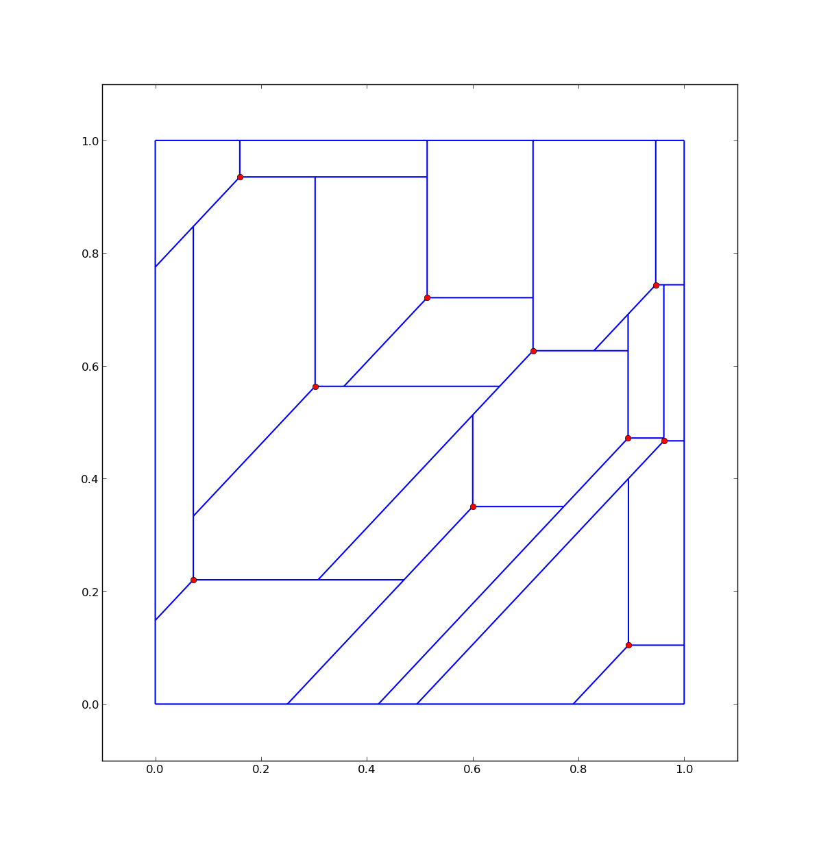
Figure 9. A simulation of the first order tropical lines process $\mathcal{G}^{1}_{L}$ with $\lambda=10$, restricted to the square $[0,1]^{2}$. The red points are the starting positions of the motorcycles, which form a Poisson point process in $\mathbb{R}^{2}$ with rate $\lambda$. The blue lines are the motorcycles’ trails.

The tropical lines process can be defined directly as an iterated Gilbert model as follows. Let $m=3$, $A$ be the set of angles $\{0,\pi/2,5\pi/4\}$ relative to $(1,0)$, called east, north and southwest directions, respectively. Let the measure $\mathcal{A}_{2}$ has mass 0, and $\mathcal{A}_{3}$ has mass 1 on the set $A$. In other words, at each point of the Poisson point process $\mathcal{P}$ with rate $\lambda>0$, put three motorcycles, one in each direction in $A$. Then $\mathcal{G}^{k}_{L}=\mathcal{G}^{k}(\mathcal{P},A)$. The exact and asymptotic intensities of the vertice, edge and face processes for the $k$-th order tropical line process $\mathcal{G}^{k}_{L}$ follow from Proposition 7.

Corollary 32.

For $k\geq 1$, let $\lambda_{0}^{k},\lambda_{1}^{k},\lambda_{2}^{k}$, be the intensities of the vertices, edges and cells of $\mathcal{G}^{k}_{L}$, respectively. Then

$$\lambda_{0}^{k} =(3k+1)\lambda,$$

$$\lambda_{1}^{k} =6k\lambda,$$

$$\lambda_{2}^{k} =(3k-1)\lambda.$$

In particular, the vertex, edge and face intensities of the scaled limit $\mathcal{G}^{\infty}_{L}$ are

$$\lambda_{0}^{\infty}=3\lambda,\hskip 5.0pt\lambda_{1}^{\infty}=2\lambda,\hskip 5.0pt\lambda_{2}^{\infty}=3\lambda.$$

Corollary 33.

Let $p_{-\cap|}$, $p_{-\cap/}$ and $p_{|\cap/}$ denote the intensities of the three types of intersections of $\mathcal{G}^{\infty}_{L}$. Then

$$p_{-\cap|}=\lambda\frac{2\sqrt{2}}{\sqrt{2}+1},\hskip 5.0ptp_{|\cap/}=p_{-\cap/}=\lambda\left(\frac{\sqrt{2}+3}{2}\right)\frac{1}{\sqrt{2}+1}.$$ (39)

Note that the intensity of intersections, $\lambda^{\infty}_{0}$, is

$$\lambda^{\infty}_{0}=\lambda\left(\frac{\sqrt{2}+3}{\sqrt{2}+1}+\frac{2\sqrt{2}}{\sqrt{2}+1}\right)=3\lambda,$$

which agrees with Corollary 32.

Proof.

By Theorem 27, $\mathcal{G}^{\infty}_{L}$ is the Poisson line process consisting of three types of lines with directions $(1,0)$, $(0,1)$ and $\frac{1}{\sqrt{2}}(-1,-1)$, with intensities $\mu_{-},\mu_{|}$ and $\mu_{/}$. We can fix different observation windows $W$ to calculate the intensity for each type of intersection. Let $\lambda=1$. For $-\cap|$, let $W$ be a square of sidelength 1. Thus,

$$p_{-\cap|}=\mu_{-}\mu_{|}=\frac{2\sqrt{2}}{\sqrt{2}+1}.$$

For $-\cap/$, let $W$ be the parallelogram formed by the vectors $(1,0)$ and $(-1,-1)$. There are $\mu_{-}$ many horizontal lines, and $\frac{1}{\sqrt{2}}\mu_{/}$ many diagonal lines crossing $W$. Thus

$$p_{-\cap/}=\frac{1}{\sqrt{2}}\mu_{-}\mu_{/}=\left(\frac{\sqrt{2}+3}{2}\right)\frac{1}{\sqrt{2}+1}.$$

The intensity of $|\cap/$ equals that of $-\cap/$ by symmetry. $\Box$

Now consider the faces of $\mathcal{G}^{k}_{L}$. The edge directions of each face are one of the three directions of $A$. One can check that each face is an ordinary and tropically convex set, that is, it is a polytrope [13]. Classifying polytropes by their combinatorial type is an interesting problem [13, 18]. Let us compute the intensities of various polytropes by their combinatorial types in $\mathcal{G}^{k}_{L}$.

Polytropes in $\mathbb{R}^{2}$ have $3,4,5$ or $6$ proper vertices. For $i=0,\ldots,3$, let $p^{k}_{i}$ denote the intensity of cells of $\mathcal{G}^{k}_{L}$ with $3+i$ vertices. Then

$$p^{k}_{0}+p^{k}_{1}+p^{k}_{2}+p^{k}_{3}=\lambda_{2}^{k}=(3k-1)\lambda.$$ (40)

Now, each point in $\Psi$ is the proper vertex of three faces, each intersection of order $3$ in $\mathcal{G}^{k}_{L}$ is the proper vertex of two faces, and each intersection of order $4$ in $\mathcal{G}^{k}_{L}$ is the proper vertex of four faces. Thus,

$$3p^{k}_{0}+4p^{k}_{1}+5p^{k}_{2}+6p^{k}_{3}=3\lambda+2\cdot 3\lambda+4\cdot 3(k-1)\lambda=(12k-3)\lambda.$$ (41)

For $p_{i}$ the intensity of cells of $\mathcal{G}^{\infty}_{L}$ with $3+i$ vertices for $i=0,1,2,3$, we have

$$p_{0}+p_{1}+p_{2}+p_{3} =3\lambda$$ (42)

$$3p_{0}+4p_{1}+5p_{2}+6p_{3} =12\lambda,$$ (43)

While (42) and 43) do not uniquely determine the intensities $p_{i}$, we can compute these numbers directly from the Poissonian description of $\mathcal{G}^{\infty}_{L}$.

Lemma 34.

Let $p_{i}$ be the intensity of cells of $\mathcal{G}^{\infty}_{L}$ with $3+i$ vertices for $i=0,1,2,3$, we have

$$p_{3} \approx 0.429367312053161, p_{4} \approx 2.22221756362048,$$

$$p_{5} \approx 0.267462936599565,\hskip 10.00002pt\mbox{ and } p_{6} \approx 0.0809521877267980.$$

Proof.

Fix a rectangle of width $x$, height $y$, with $x>y$. Let $N_{a}$, $N_{b}$ and $N_{c}$ be the number of diagonal lines crossing regions $A,B,C$ in Figure 10 below. Note that these are independent Poisson random variables, with means $a=\min(x,y)/\sqrt{2}$, $b=|y-x|/\sqrt{(}2)$ and $c=a$, respectively. Conditioned on the values of $N_{a}$, $N_{b}$ and $N_{c}$, we can count the number of triangles, quadilaterals, pentagons and hexagons generated. See Table 1.

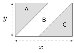
Figure 10. An $x\times y$ rectangle with $x>y$ is divided into three regions labelled $A,B$ and $C$ by two diagonal lines. Conditioned on the number of diagonal lines of $\mathcal{G}^{\infty}_{L}$ hitting each region, one can compute the intensities of faces of $\mathcal{G}^{\infty}_{L}$ by vertices.

$N_{a}$	$N_{b}$	$N_{c}$	$\triangle$	$\square$	⬠	⬡
0	0	0	0	1	0	0
1	0	0	1	0	1	0
0	0	1	1	0	1	0
$\geq 1$	0	$\geq 1$	2	$N_{a}+N_{c}-2$	0	1
0	$\geq 1$	0	0	$N_{b}+1$	0	0
1	$\geq 1$	0	1	$N_{b}$	0	0
0	$\geq 1$	1	1	$N_{b}$	0	0
$\geq 1$	$\geq 1$	$\geq 1$	2	$N_{a}+N_{b}+N_{c}-3$	2	0

Table 1. Number of polytropes of each type generated by a single rectangle, conditioned on the number of diagonal lines intersecting it.

Let $i$ be an index variable taking values in $\{3,4,5,6\}$. Using the previous table, for each fixed rectangle of size $x\times y$, we can compute $e_{i}(x,y)$, the expected number of polytropes with $i$ vertices. Now fix a large square $W$ of side length $s$. Consider the Manhattan line process with horizontal and vertical intensities $\mu_{-}$. There are $s^{2}\mu_{-}^{2}+o(s^{2})$ many rectangles in $W$. The side lengths of the rectangles are distributed as i.i.d. exponential with mean $1/\mu_{-}$. Then

$$s^{2}\int_{x,y}e_{i}(x,y)e^{-\mu_{-}(x+y)}\,dx\,dy+o(s^{2})$$

is the expected number of polytropes with $i$ vertices in $W$. Thus, as $s\to\infty$, the density of polytropes with $i$ vertices is precisely

$$p_{i}=\int_{x,y}e_{i}(x,y)e^{-\mu_{-}(x+y)}\,dx\,dy$$

for $i\in\{3,4,5,6\}$. Numerically evaluate these integrals yield the result. $\Box$

5. Discussions

Our work leaves a number of open questions for both algebraic and stochastic geometers. To be concrete, we list a few such problems:

1. Is there a distributional limit for the error term $d\left(\mathcal{G}^{k}\left(\frac{1}{k}\right)\cap W,\mathcal{G}^{\infty}\cap W\right)$, where $d$ is some distance between sets? For a classical Poisson line process, the fluctuations of such statistics around the limit are Gaussian. In this case, we have extra fluctuations from the Gilbert iterations. We suspect that the fluctuations are still Gaussian, but with higher variance.

2. What happens when the number of angles $A$ is not finite? For example, what is the limit of the iterated classical Gilbert tessellation with uniform angle distribution on $[0,\pi]$?

3. What happens when the underlying point process $\mathcal{P}$ is stationary but not Poisson? In particular, for what types of point processes beyon Poisson are the dilation scaling results obtained here still valid?

4. What happens to systems of tropical polynomials in higher variables? The intersections would now be segments of hyperplanes of various codimensions. These processes will also be dense, and thus one needs a way to enumerate the common zeros. However, it is not clear what is the effective analogue of the iterated Gilbert tessellation in higher dimensions.

5. Is the Poisson tropical plane curve process the tropicalization of some processes of classical varieties? Tropicalization is often studied in the field of Puiseux series, or the $p$-adics. There has been work by Evans [10] on systems of polynomials whose coefficients are $p$-adic Gaussians. However, their tropicalizations would result in discretely distributed coefficients, and thus the current result does not directly apply.

Appendix

In this section, we first review some basics of stochastic geometry, give the precise definitions of the terms and the proof of these propositions.

Background

We first review some terminologies in stochastic geometry, for reference see [16] and [8]. For a set $\{\cdot\}$, let $\text{Card}\{\cdot\}$ denote its cardinality. For $V\subset\mathbb{R}^{2}$ and $x\in\mathbb{R}^{2}$, let $x+V$ be the translated set $\{x+y:y\in V\}$. Let $\mathcal{C}$ denote the set of closed sets in $\mathbb{R}^{2}$. Let $\mathcal{C}^{1}\subset\mathcal{C}$ be the set of tropical curves with finite and positive degrees. Note that when we write $V_{f}\in\mathcal{C}^{1}$, we view the tropical curve $V_{f}$ as a closed set in $\mathbb{R}^{2}$. In contrast, when we write $V_{f}\in\mathcal{V}$, we view it as a compact set with marked points. For notational convenience, we will suppress the dependence on $f$ and write $V_{n}$ for $V_{f_{n}}$. Let $\mathcal{B}$ denote the Borel $\sigma$-algebra of the Fell topology on $\mathcal{C}$. A point process on $\mathcal{C}^{1}$ is a counting measure of the form

$$\Phi=\Phi(\omega)=\sum_{n\in\mathbb{N}}\delta_{V_{n}},$$ (44)

that satisfies the following $\sigma$-finiteness (or Radon) condition: for all compact sets $K\subset\mathbb{R}^{2}$,

$$\mbox{Card}\{n\mbox{ s.t. }V_{n}\cap K\neq\emptyset\}<\infty,\quad\mathbb{P}\mbox{-a.s.}.$$ (45)

Here $V_{n}$ are random variables taking values in $\mathcal{C}^{1}$, that is, they are random tropical curves. The intensity measure $\Lambda$ of $\Phi$ is the measure on $\mathcal{B}$ given by

$$\Lambda(A)=\mathbb{E}(\Phi(A))\mbox{ for }A\in\mathcal{B}.$$

Say that $\Phi$ is a non-degenerate point process of tropical plane curves if $\Lambda$ is supported on $\mathcal{C}^{1}$. Say that $\Phi$ is stationary if its distribution is invariant under actions by the group of translations of $\mathbb{R}^{2}$. Say that $\Phi$ has positive intensity if for all compact sets $K$ of $\mathbb{R}^{2}$ with positive Lebesgue measure,

$$\mathbb{E}\left(\mbox{Card}\{n\mbox{ s.t. }V_{n}\cap K\neq\emptyset\}\right)>0.$$

If $\Phi$ satisfies the last three properties, that is, it is a non-degenerate, stationary point process of tropical plane curves with positive intensity, then we say that $\Phi$ is a stationary point process of tropical plane curves.

For a centroid function $c$ on tropical curves, one can associate with $\Phi$ the point process of centroids

$$\Psi=\sum_{n\in\mathbb{N}}\delta_{C_{n}},$$ (46)

where each $C_{n}$ is a random variable in $\mathbb{R}^{2}$, $C_{n}(\omega)=c(V_{n}(\omega))$, the centroid of the tropical plane curve $V_{n}(\omega)$. We are now ready to prove Proposition 29.

Proof of Proposition 29..

The proof is by contradiction. Assume there exists

$$\Phi=\Phi(\omega)=\sum_{n}\delta_{V_{n}},$$

which is Radon and stationary in the sense defined above. Consider the map $c:\mathcal{C}^{1}\to\mathbb{R}^{2}$, where $c(V_{n})$ is the apex of the horizontal arm of $V_{n}$ whose apex has minimum $y$-coordinate. This function is well-defined, measurable and translation invariant, therefore it is a centroid function on $\mathcal{C}^{1}$. Let $\Psi$ be the centroid point process of $\Phi$ with centroid function $c$. Since $\Phi$ is stationary and has positive intensity, and each curve in $\Phi$ yields precisely one point in $\Psi$, $\Psi$ is a stationary point process in $\mathbb{R}^{2}$ with positive intensity.

We now claim that

$$\mathbb{P}(\Psi((-\infty,0]\times[0,1])=\infty)>0.$$ (47)

The projection on the abscissa axis of the restriction of $\Psi$ to the set $(-\infty,\infty)\times[0,1])$ forms a stationary point process on $\mathbb{R}$. If (47) is not true, then it follows from the last observation and from Property 1.1.2 in [1] that

$$\mathbb{P}(\Psi((-\infty,\infty)\times[0,1])=0)=1,$$

which in turns implies that

$$\mathbb{P}(\Psi((-\infty,\infty)\times[n,n+1])=0)=1,$$

for all $n\in\mathbb{Z}$, so that

$$\mathbb{P}(\Psi(\mathbb{R}^{2})=0)=1,$$

and this contradicts the fact that the intensity of $\Psi$ is positive. So (47) must holds.

Now, each tropical curve with centroid in $(-\infty,0]\times[0,1])$ has at least one arm extending in the $(1,0)$ direction starting from this centroid point. Therefore, this arm intersects the $[(0,0),(0,1)]$ segment of $\mathbb{R}^{2}$. Hence, with positive probability, there is an infinite number of different horizontal arms of tropical lines of $\Phi$ that intersect $[(0,0),(0,1)]$. This contradicts (45). $\Box$

The second view

Alternatively, one could start with a stationary point process $\Psi$ in $\mathbb{R}^{2}$ as given in (46), and to each point $C_{n}$ attach a random tropical plane curve, translated to have $C_{n}$ as the centroid. One could then consider the set

$$\Xi=\Xi(\omega)=\bigcup_{n}V_{n}(\omega),$$ (48)

where $V_{n}(\omega)$ has centroid $C_{n}(\omega)$. If it exists, $\Xi$ would be a random variable taking values in $\mathcal{C}$. As the following example shows, it is possible to have $\Xi$ to be a well defined stationary random closed set, whereas as we know from the last lemma that the associated process $\Phi=\sum_{n}\delta_{V_{n}}$ is not a point process on $\mathcal{C}$.

Example 35.

Choose the centroid function $c$ as in the proof of Proposition 29. The centroid of a tropical line of the form $a\odot x\oplus b\odot y\oplus c$ is just the only point on its body, which is $(c-a,c-b)$. In (48), take $n=(k,l)$ varying over $\mathbb{Z}^{2}$, and for $T_{k,l}$ with $k,l\in\mathbb{Z}$, take the tropical line with centroid $(k,l)+U$, where $U$ is a random variable which is uniformly distributed in the cube $[0,1]\times[0,1]$. The associated $\Xi$ is depicted in Figure 11.

Figure 11. An instance of $\Xi$

There is no contradiction with Proposition 29. A direct evaluation shows that the centroid point process $\Psi$ has intensity 1, and that with probability 1, the number of tropical lines that intersect the $[(0,0),(0,1)]$ segment of $\mathbb{R}^{2}$ is infinite. However, all vertical (resp. horizontal or diagonal) arms that intersect this segment do so at the same point. This is of course directly linked to this specificity of this example where each tropical line has a degenerate intersection with an infinite number of other tropical lines of $\Xi$.

To rule out pathological cases as that in Example 35, we shall consider tropical curves with non-degenerate intersections. Say that two tropical curves $V,V^{\prime}$ have non-degenerate intersections, if $V\cap V^{\prime}$ is a set of finitely many points in $\mathbb{R}^{2}$. In algebraic terms, this means the corresponding system of two polynomials in two variables is not singular. For a collection $\{V\}$ of tropical curves, the union of their pairwise intersections is called the set of common zeros of $\{V\}$. If $\{V\}$ is a $\mathbb{P}$-a.s. non-degenerate collection of tropical curves, the set of common zeros is a point process in $\mathbb{R}^{2}$. We call this the intersection process of $\{V\}$, denoted by $\mathcal{I}$.

In Example 35, the set of common zeros of the collection of lines of $\Xi$ is the random closed set $\Xi$ itself, which is not the support of a point process on $\mathbb{R}^{2}$, as it contains lines. Unfortunately, as claimed in Proposition 30, we cannot define $\Xi$ such that both the associated centroid process and the intersection process are stationary with positive intensities.

Proof of Proposition 30.

Consider the maps $c_{1},c_{2}:\mathcal{C}^{1}\to\mathbb{R}^{2}$, where $c_{1}(V)$ is the apex of the horizontal arm of $T$ with minimum $y$-coordinate, and $c_{2}(V)$ is the apex of the vertical arm of $T$ with minimum $x$-coordinate. As argued in the proof of Proposition 29, both of these are centroid functions of tropical curves.

Consider the set $\Xi$ defined in (48) via some stationary, positive intensity centroid point process $\Psi$. Let $\Psi_{1}$ be the centroid process of $\Xi$ associated with the function $c_{1}$, $\Psi_{2}$ be the centroid process of $\Xi$ associated with the function $c_{2}$. There is a bijection between points of $\Psi$, $\Psi_{1}$ and $\Psi_{2}$ via the tropical curves $T_{n}$. Since centroid functions are translation invariant, and since $\Psi$ is a stationary point process with positive intensity, it follows that $\Psi_{1}$ and $\Psi_{2}$ are also.

Now, either

$$\mathbb{P}(\exists m\neq n\mbox{ s.t. }V_{m}\mbox{ and }V_{n}\mbox{ have degenerate intersection})>0$$

in which case the set of common zeros contains a half line with positive probability, and the result follows. Or

$$\mathbb{P}(\exists m\neq n\mbox{ s.t. }V_{m}\mbox{ and }V_{n}\mbox{ have degenerate intersection})=0.$$

Consider this second case. Let

$$\tau_{1}=\{V_{n}:c_{1}(V_{n})\in(-\infty,0]\times[0,1]\},$$

and

$$\tau_{2}=\{V_{n}:c_{2}(V_{n})\in[-1,0]\times(-\infty,0]\}.$$

Apply the argument in Proposition 29 to $\Psi_{1}$, we get

$$\mathbb{P}(\mbox{Card}(\tau_{1})=\infty)>0.$$ (49)

Since $\Psi_{2}$ has positive intensity,

$$\mathbb{P}(\mbox{Card}(\tau_{2})>0)=1.$$ (50)

Each $V_{n}=V_{f_{n}}$ is dual to the subdivision of the triangle with vertices $(0,0),(0,d),(d,0)$, where $d$ is the degree of $f_{n}$. Therefore, by definition of $c_{1}$ and $c_{2}$, the $y$-coordinate of $c_{1}(V_{n})$ is at most the $y$-coordinate of $c_{2}(V_{n})$, and the $x$-coordinate of $c_{2}(V_{n})$ is at most the $x$-coordinate of $c_{1}(V_{n})$. Therefore, it is not possible for a tropical curve to be in both $\tau_{1}$ and $\tau_{2}$.

Let

$$I=\bigcup_{V_{n}\in\tau_{1},V_{m}\in\tau_{2}}V_{n}\cap V_{m}$$

be the subset of the set of common zeros which are intersections of pairs of tropical lines in $\tau_{1}$ and $\tau_{2}$. Since such intersections are a.s. non-degenerate, $I$ must be a collection of points in $[-1,0]\times[0,1]$. By definition of $c_{1}$, for each point in $c_{1}$, there is a tropical curve $V_{n}$ with a horizontal arm ($(1,0)$ direction) starting from this point. Similarly, for each point in $c_{2}$, there is a tropical curve $V_{m}$ with a vertical arm ($(0,1)$ direction) starting from this point. Thus, each set $V_{n}\cap T_{m}$ necessarily contains a point $p_{mn}\in[-1,0]\times[0,1]$ that is the intersection of this horizontal and vertical arms.

By the non-degenerate intersection assumption, $\mathbb{P}$-a.s. there are no two tropical plane curves with identical $c_{1}$-centroids or $c_{2}$-centroids. Therefore,$p_{mn}\neq p_{m^{\prime}n^{\prime}}$ whenever either $m\neq m^{\prime}$ or $n\neq n^{\prime}$. That is, all the intersections from different pairs are different.

Thus, by (49) and (50),

$$\mathbb{P}(\mbox{Card}(I)=\infty)>0.$$

Hence, the set of common zeros of $\Xi$ cannot be Radon in this case too. $\Box$

References

- [1] Francois Baccelli and Pierre Brémaud. Elements of queueing theory: Palm Martingale calculus and stochastic recurrences, volume 26. Springer Science & Business Media, 2013.
- [2] Francois Baccelli and Ngoc Mai Tran. Zeros of random tropical polynomials, random polygons and stick-breaking. Transactions of the American Mathematical Society, 368(10):7281–7303, 2016.
- [3] James Burridge, Richard Cowan, and Isaac Ma. Full-and half-Gilbert tessellations with rectangular cells. Advances in Applied Probability, 45(01):1–19, 2013.
- [4] Codina Cotar, Alexander E Holroyd, and David Revelle. A percolating hard sphere model. Random Structures & Algorithms, 34(2):285–299, 2009.
- [5] Codina Cotar and Stanislav Volkov. A note on the lilypond model. Advances in Applied Probability, 36(2):325–339, 2004.
- [6] Daryl Daley. Further results for the lilypond model. Spatial Point Process Modelling and Its Applications, 20:55, 2004.
- [7] Daryl Daley and Günter Last. Descending chains, the lilypond model, and mutual-nearest-neighbour matching. Advances in applied probability, pages 604–628, 2005.
- [8] Daryl Daley and David Vere-Jones. An introduction to the theory of point processes: volume II: general theory and structure. Springer Science & Business Media, 2007.
- [9] David Eppstein, Michael T Goodrich, Ethan Kim, and Rasmus Tamstorf. Motorcycle graphs: canonical quad mesh partitioning. In Computer Graphics Forum, volume 27, pages 1477–1486. Wiley Online Library, 2008.
- [10] Steven N Evans. The expected number of zeros of a random system of-adic polynomials. Electronic Communications in Probability [electronic only], 11:278–290, 2006.
- [11] Olle Häggström and Ronald Meester. Nearest neighbor and hard sphere models in continuum percolation. Random Structures & Algorithms, 9(3):295–315, 1996.
- [12] Matthias Heveling and Günter Last. Existence, uniqueness, and algorithmic computation of general lilypond systems. Random Structures & Algorithms, 29(3):338–350, 2006.
- [13] Michael Joswig and Katja Kulas. Tropical and ordinary convexity combined. Advances in geometry, 10(2):333–352, 2010.
- [14] Günter Last and Mathew D Penrose. Percolation and limit theory for the poisson lilypond model. Random Structures & Algorithms, 42(2):226–249, 2013.
- [15] Diane Maclagan and Bernd Sturmfels. Introduction to tropical geometry, volume 161. American Mathematical Soc., 2015.
- [16] Rolf Schneider and Wolfgang Weil. Stochastic and integral geometry. Springer Science & Business Media, 2008.
- [17] Tomasz Schreiber and Natalia Soja. Limit theory for planar gilbert tessellations. arXiv preprint arXiv:1005.0023, 2010.
- [18] Ngoc Mai Tran. Enumerating polytropes. arXiv preprint arXiv:1310.2012, 2013.