Charm Quark Mass with Calibrated Uncertainty

Abstract

We determine the charm quark mass $\hat{m}_{c}$ from QCD sum rules of moments of the vector current correlator calculated in perturbative QCD at ${\cal O}(\hat{\alpha}_{s}^{3})$. Only experimental data for the charm resonances below the continuum threshold are needed in our approach, while the continuum contribution is determined by requiring self-consistency between various sum rules. Existing data from the continuum region can then be used to bound the theoretic uncertainty. Our result is $\hat{m}_{c}(\hat{m}_{c})=1272\pm 8$ MeV for $\hat{\alpha}_{s}(M_{Z})=0.1182$.

MITP/16-087

1 Introduction

As a fundamental parameter of the Standard Model (SM) of particle physics that enters the calculation of many physical observables, it is important to determine the charm quark mass as accurately as possible and by using several different methods. Moreover, it is one of the central goals of future high-energy lepton colliders to measure the charm quark Yukawa coupling to sub-percent precision in order to test the mass-coupling relation, as predicted in the minimal SM with a single Higgs doublet. Thus, the precision in the charm quark mass should at least match and ideally surpass that in the charm Yukawa coupling.

Most recent determinations [1] of the $\overline{\rm MS}$ charm quark mass, $\hat{m}_{c}(\mu=\hat{m}_{c})$, including all of the most precise ones, rely on either lattice simulations or variants of QCD sum rules [2, 3, 4]. Both approaches are based on rigorous field theoretical principles and can be systematically improved. Nevertheless, the resulting uncertainties are dominated by theory errors which are notoriously difficult to estimate and often subject of vigorous debate.

The goal of this article is then to revisit the relativistic sum rule method with emphasis on the evaluation of the uncertainty and specifically to show that the overall error may also be constrained within our approach. To this end, we will adopt a strategy where the only exploited experimental information are the masses and electronic decay widths of the narrow resonances in the sub-continuum charm region, $J/\Psi$ and $\Psi(2S)$. Consistency between different QCD sum rules will be seen to suffice to constrain the continuum of charm pair production with good precision. For this procedure to work it is crucial to include alongside the first and higher moment sum rules also the zeroth moment, as the latter exhibits enhanced sensitivity to the continuum. Comparison with existing data on the $R$-ratio for hadronic relative to leptonic final states in $e^{+}e^{-}$ annihilation will then serve as a control, providing an independent error estimate which we interpret as the error on the method and add it as an additional error contribution. In this way, we can show that the overall precision in $\hat{m}_{c}$ from relativistic sum rules is at the sub-percent level.

Specifically, there are two sources of uncertainty which are particularly difficult to quantify, and therefore occasionally not even included in the error budget. One are condensate contributions within the operator product expansion (OPE) beyond the leading gluon condensate term. The other issue is quark-hadron duality: Formally, the sum rule is based on the optical theorem, where the real part of the correlator is evaluated theoretically with quark and gluon degrees of freedom, while the imaginary part involves as dual degrees of freedom the hadrons observed in experiments. While such a global change of variables is highly non-trivial, it is innocuous as long as one does not mix these descriptions on either side of the sum rule. As far as the evaluation of the imaginary part is concerned, one is forced, however, to switch at some specific point in the squared energy $s$ from experimental data to perturbative QCD since in practice data are necessarily constrained to a finite region while the upper integration limit is unbounded. In this way one has to rely on local quark-hadron duality which – at least as a matter of principle – is unjustified. Still, as long as $s$ is large enough, one introduces little additional uncertainty. Now, the largest value of $\sqrt{s}$ for which data of the total hadronic cross section in $e^{+}e^{-}$ annihilation are available (see the data points in Figure 5 in Section 3) is 5 GeV, and beyond $\sqrt{s}=4.6$ GeV data points are scarce and have very large errors. Around this energy there is still considerable fluctuations in the measured cross-section, shedding some doubt on the applicability of local quark-hadron duality even in practice. One of the features of our work is that it merely relies on quark-hadron duality in a finite region, namely between the $\psi(2S)$ resonance and the continuum threshold. While this is still not rigorously justified, it should largely mitigate the aforementioned problem. Furthermore, by using continuum data only as a calibration of the uncertainty, we control the error associated with the necessary deviation from strict global quark-hadron duality.

The paper is organized as follows. In the next section we review the formalism following Ref. [5] and describe how self-consistency between moments of the current correlator allows us to constrain the continuum region and determine a precise value of the charm quark mass. This section will already contain our main result, $\hat{m}_{c}(\hat{m}_{c})=1272\pm 8$ MeV for $\hat{\alpha}_{s}(M_{Z})=0.1182$. In Section 3 we add a detailed discussion of the influence of the continuum region using experimental data and confirm the validity of the result of Section 2. Section 4 offers details of a more general fit procedure where parameter uncertainties can be taken into account in a more systematic way, and we also include a comparison with earlier results. We summarize in Section 6.

2 Formalism and charm-mass determination

We consider the transverse part of the correlator $\hat{\Pi}_{q}(t)$ of two heavy-quark vector currents where the caret indicates $\overline{\rm MS}$ subtraction. $\hat{\Pi}_{q}(t)$ can be calculated in perturbative QCD (pQCD) order by order and obeys the subtracted dispersion relation [6]

$$12\pi^{2}\frac{\hat{\Pi}_{q}(0)-\hat{\Pi}_{q}(-t)}{t}=\int_{4\hat{m}_{q}^{2}}^{\infty}\frac{{\rm d}s}{s}\frac{R_{q}(s)}{s+t}\ ,$$ (1)

where $R_{q}(s)=12\pi\mbox{Im}\hat{\Pi}_{q}(s)$, and $\hat{m}_{q}=\hat{m}_{q}(\hat{m}_{q})$ is the mass of the heavy quark. In the limit $t\rightarrow 0$, Eq. (1) coincides with the first moment, ${\cal M}_{1}$, of $\hat{\Pi}_{q}(t)$. In general, there is a sum rule for each higher moment as well [2, 3, 4],

$${\cal M}_{n}:=\left.\frac{12\pi^{2}}{n!}\frac{d^{n}}{dt^{n}}\hat{\Pi}_{q}(t)\right|_{t=0}=\int_{4\hat{m}_{q}^{2}}^{\infty}\frac{{\rm d}s}{s^{n+1}}R_{q}(s).$$ (2)

Taking the opposite limit of Eq. (1), i.e. $t\rightarrow\infty$, multiplying with $t$ and properly regularizing, one can also define a sum rule for the $0^{th}$ moment [5]. ${\cal M}_{0}$ is then obtained from the dispersion relation for the difference $\hat{\Pi}_{q}(0)-\hat{\Pi}_{q}(-t)$ where the (unphysical) constant $\hat{\Pi}_{q}(0)$ is subtracted, tantamount to the definition of higher moments as derivatives of $\hat{\Pi}_{q}(-t)$. At a given order in pQCD, the required regularization can be obtained by subtracting the zero-mass limit of $R_{q}(s)$, which we write as $3Q_{q}^{2}\lambda_{1}^{q}(s)$ with $Q_{q}$ the quark charge. $\lambda_{1}^{q}(s)$ is known up to ${\cal O}(\hat{\alpha}_{s}^{4})$, but we will only need the third-order expression [7],

$$\lambda^{q}_{1}(s) = 1+\frac{\hat{\alpha}_{s}}{\pi}+\frac{\hat{\alpha}_{s}^{2}}{\pi^{2}}\left[\frac{365}{24}-11\zeta(3)+n_{q}\left(\frac{2}{3}\zeta(3)-\frac{11}{12}\right)\right]$$

$$+ \frac{\hat{\alpha}_{s}^{3}}{\pi^{3}}\left[\frac{87029}{288}-\frac{121}{8}\zeta(2)-\frac{1103}{4}\zeta(3)+\frac{275}{6}\zeta(5)\right.$$

$$+ \left.n_{q}\left(-\frac{7847}{216}+\frac{11}{6}\zeta(2)+\frac{262}{9}\zeta(3)-\frac{25}{9}\zeta(5)\right)+n_{q}^{2}\left(\frac{151}{162}-\frac{\zeta(2)}{18}-\frac{19}{27}\zeta(3)\right)\right],$$

where $\hat{\alpha}_{s}=\hat{\alpha}_{s}(\sqrt{s})$, $n_{q}=n_{l}+1$ and $n_{l}$ is the number of light flavors (taken as massless), i.e., quarks with masses below the heavy quark under consideration.

$R$	$M_{R}$ [GeV]	$\Gamma_{R}^{e}$ [keV]
$J/\Psi$	3.096916	5.55(14)
$\Psi(2S)$	3.686109	2.361(4)

Table 1: Resonance data [8] used in the analysis. The uncertainties from the resonance masses are negligible for our purpose.

By the optical theorem, $R_{q}(s)$ can be related to the measurable cross section for heavy-quark production in $e^{+}e^{-}$ annihilation. Below the threshold for continuum heavy-flavor production, the cross section is determined by a small number of narrow Breit-Wigner resonances [2], approximated by $\delta$-functions,

$$R_{q}^{\rm Res}(s)=\frac{9\pi}{\alpha_{\rm em}^{2}(M_{R})}M_{R}\Gamma_{R}^{e}\delta(s-M_{R}^{2}).$$ (4)

The masses $M_{R}$ and electronic widths $\Gamma^{e}_{R}$ of the resonances [8] needed for the determination of the charm mass are listed in Table 1 and $\alpha_{\rm em}(M_{R})$ is the running fine structure constant at the resonance.

We invoke global quark-hadron duality, and we assume that continuum production can be described on average by the simple ansatz [5],

$$R_{q}^{\rm cont}(s)=3Q^{2}_{q}\lambda^{q}_{1}(s)\sqrt{1-\frac{4\,\hat{m}_{q}^{2}(2M)}{s^{\prime}}}\left[1+\lambda^{q}_{3}\frac{2\,\hat{m}_{q}^{2}(2M)}{s^{\prime}}\right],$$ (5)

where $s^{\prime}:=s+4(\hat{m}_{q}^{2}(2M)-M^{2})$, and $M$ is taken as the mass of the lightest pseudoscalar charmed meson, i.e., $M=M_{D^{0}}=1864.84$ MeV [8]. $\lambda^{q}_{3}$ is a free parameter to be determined. $R_{q}^{\rm cont}(s)$ interpolates smoothly between the threshold and the onset of open heavy-quark pair production and coincides asymptotically with the prediction of pQCD for massless quarks.

$n$	$C_{n}^{(0)}$	$C_{n}^{(1)}$	$C_{n}^{(2)}$	$C_{n}^{(3)}$
$1$	$1.0667$	$2.5547$	$2.4967$	$-5.6404$
$2$	$0.4571$	$1.1096$	$2.7770$	$-3.4937$
$3$	$0.2709$	$0.5194$	$1.6388$	$-2.8395$
$4$	$0.1847$	$0.2031$	$0.7956$	$-3.722\pm 0.500$
$5$	$0.1364$	$0.0106$	$0.2781$	$-4.425\pm 1.200$

Table 2: The coefficients $C_{n}^{(i)}$ for the perturbative expansion of the QCD moments, Eq. (8, 9), as used in this work. The first line for $n=$1 is taken from Ref. [14], the coefficients for $n=2$, 3 from [17] and the last ones for $n=4$, 5 from Ref. [20].

Using the results of Refs. [10, 11] and $R_{q}(s)=\sum\limits_{\rm resonances}R_{q}^{\rm Res}(s)+R_{q}^{\rm cont}(s)$, the sum rule for ${\cal M}_{0}$ obtained from Eq. (1) in the limit $t\rightarrow\infty$ and dividing by $3Q_{q}^{2}$ reads explicitly,

$$\sum\limits_{\rm resonances}\frac{9\pi\Gamma^{e}_{R}}{3Q_{q}^{2}M_{R}\alpha_{em}^{2}(M_{R})}+\int\limits_{4M^{2}}^{\infty}\frac{{\rm d}s}{s}\left(\frac{R_{q}^{\rm cont}(s)}{3Q_{q}^{2}}-\lambda_{1}^{q}(s)\right)-\int\limits_{\hat{m}_{q}^{2}}^{4M^{2}}\frac{{\rm d}s}{s}\lambda^{q}_{1}(s)$$

$$=-\frac{5}{3}+\frac{\hat{\alpha}_{s}}{\pi}\left[4\zeta(3)-\frac{7}{2}\right]$$ (6)

$$\quad+\left(\frac{\hat{\alpha}_{s}}{\pi}\right)^{2}\left[\frac{2429}{48}\zeta(3)-\frac{25}{3}\zeta(5)-\frac{2543}{48}+n_{q}\left(\frac{677}{216}-\frac{19}{9}\zeta(3)\right)\right]+\left(\frac{\hat{\alpha}_{s}}{\pi}\right)^{3}A_{3}\ ,$$

$$=-1.667+1.308\,\frac{\hat{\alpha}_{s}}{\pi}+1.595\left(\frac{\hat{\alpha}_{s}}{\pi}\right)^{2}-8.427\left(\frac{\hat{\alpha}_{s}}{\pi}\right)^{3}\,,$$

where $\hat{\alpha}_{s}=\hat{\alpha}_{s}(\hat{m}_{q})$ and the third-order coefficient $A_{3}$ is available in numerical form [12, 13],

$$A_{3}=-9.863+0.399\,n_{q}-0.010\,n_{q}^{2}\ .$$ (7)

In the last line of Eq. (6) we show numerical values for the case of charm quarks, i.e. $n_{q}=4$, exhibiting a marked breakdown of convergence of the perturbative expansion. Notice that the continuum $R_{q}^{\rm cont}(s)$ contributes with the lower integration limit $4M^{2}$, while the subtraction term $\lambda_{1}^{q}(s)$ is integrated starting from $\hat{m}_{q}^{2}$. We reiterate that this definition of ${\cal M}_{0}$ does not involve the unphysical constant $\hat{\Pi}_{q}(0)$ separately, but only the difference $\hat{\Pi}_{q}(0)-\hat{\Pi}_{q}(-t)$.

$n$	$a_{n}$	$b_{n}$
$0$	$-\frac{2}{15}$	$\frac{605}{162}$
$1$	$-\frac{32}{105}$	$\frac{32099}{12960}$
$2$	$-\frac{32}{63}$	$\frac{59}{56}$
$3$	$-\frac{512}{693}$	$-\frac{20579}{42525}$
$4$	$-\frac{1280}{1287}$	$-\frac{100360567}{47628000}$
$5$	$-\frac{8192}{6435}$	$-\frac{459884251}{121080960}$

Table 3: The coefficients $a_{n}$ and $b_{n}$ needed to calculate the contribution from the dimension-4 gluon condensate to the QCD moments, Eq. (10). The numbers are taken from Refs. [21, 22, 23].

Eq. (6) contains two unknowns, the quark mass $\hat{m}_{q}(\hat{m}_{q})$ and the parameter $\lambda_{3}^{q}$ entering in our prescription for $R_{q}^{\rm cont}(s)$. The zeroth sum rule is the most sensitive to the continuum region and therefore to $\lambda_{3}^{q}$, while the other moments mostly determine the quark mass.

Theory predictions for the higher moments in perturbative QCD can be cast into the form

$${\cal M}_{n}^{\rm pQCD}=\frac{9}{4}Q_{q}^{2}\left(\frac{1}{2\hat{m}_{q}(\hat{m}_{q})}\right)^{2n}\hat{C}_{n}$$ (8)

with

$$\hat{C}_{n}=C_{n}^{(0)}+\left(\frac{\hat{\alpha}_{s}}{\pi}+\frac{3Q_{q}^{2}\alpha_{\rm em}}{4\pi}\right)C_{n}^{(1)}+\left(\frac{\hat{\alpha}_{s}}{\pi}\right)^{2}C_{n}^{(2)}+\left(\frac{\hat{\alpha}_{s}}{\pi}\right)^{3}C_{n}^{(3)}+{\cal O}(\hat{\alpha}_{s}^{4})\,.$$ (9)

The $C_{n}^{(i)}$ are known up to ${\cal O}(\hat{\alpha}_{s}^{3})$ for $n\leq 3$ [14, 15, 16, 17], and up to ${\cal O}(\hat{\alpha}_{s}^{2})$ for the rest [18, 19]. For the convenience of the reader we collect the numerical values of the coefficients $C_{n}^{(i)}$ required for our analysis in Table 2. Since we evaluate the moments up to ${\cal O}(\hat{\alpha}_{s}^{3})$ we use the predictions for $n>3$ provided in Ref. [20]. The QED contribution to the QCD moments proportional to $\alpha_{\rm em}/\pi$ is very small and it is sufficient to include the first-order term.

$n$	Resonances	Continuum	Total	Theory
0	1.231 (24)	$-3.229(+28)(43)(1)$	$-1.999(56)$	Input (11)
1	1.184 (24)	$0.966(+11)(17)(4)$	$2.150(33)$	2.169(16)
2	1.161 (25)	$0.336(+5)(8)(9)$	$1.497(28)$	Input (25)
3	1.157 (26)	$0.165(+3)(4)(16)$	$1.322(31)$	1.301(39)
4	1.167 (27)	$0.103(+2)(2)(26)$	$1.270(38)$	1.220(60)
5	1.188 (28)	$0.080(+1)(1)(38)$	$1.268(47)$	1.175(95)

Table 4: Results for the lowest moments, ${\cal M}_{n}$, defined in Eq. (6) for $n=0$ (multiplied by $3Q_{q}^{2}$) and Eq. (2) for $n\geq 1$ and including the contribution from the gluon condensate, Eq. (10) (multiplied by $10^{n}\,\mbox{GeV}^{2n}$). The first error for the continuum part is obtained from shifting the central value $\lambda_{3}^{c}=1.23$ (determined from the 0th and the 2nd moment) to $\lambda_{3}^{c,{\rm exp}}=1.34(17)$ (determined from fixing the 0th moment by experimental data, see next section). The second error is propagated from the experimental uncertainties of data in the threshold region, $\Delta\lambda_{3}^{c,{\rm exp}}=\pm 0.17$. The third error is due to the uncertainty of the gluon condensate. The errors for the sum of the resonance and continuum parts (denoted ’Total’ in column 4) combines all errors in quadrature. The last column shows the theoretical predictions using Eq. (8) for $\hat{m}_{c}(\hat{m}_{c})=1.272$ GeV and $\hat{\alpha}_{s}(M_{Z})=0.1182$ [25] with the truncation error determined from Eq. (12).

In general, vacuum expectation values of higher-dimensional operators in the OPE contribute to the moments of the current correlator as well. These condensates may be important for a high-precision determination of heavy-quark masses, in particular in the case of the charm quark. The leading term involves the dimension-4 gluon condensate [2],

$${\cal M}^{\rm cond}_{n}=\frac{12\pi^{2}Q_{q}^{2}}{(4\hat{m}_{q}^{2})^{n+2}}\left\langle\frac{\hat{\alpha}_{s}}{\pi}G^{2}\right\rangle\,a_{n}\left(1+\frac{\hat{\alpha}_{s}(\hat{m}_{q})}{\pi}b_{n}\right)\,.$$ (10)

The coefficients $a_{n}$ and $b_{n}$ can be found in Refs. [21, 22, 23] and are collected in Table 3. We will use $C_{G}^{\rm exp}:=\langle\frac{\hat{\alpha}_{s}}{\pi}G^{2}\rangle^{\rm exp}=0.005$ GeV⁴ as our central value and assume a 100% uncertainty, $\Delta_{G}=0.005$ GeV⁴, taken from the recent analysis [24].

$n$	$\frac{\Delta{\cal M}_{n}^{(2)}}{\left|{\cal M}_{n}^{(2)}\right|}$	$\frac{\Delta{\cal M}_{n}^{(3)}}{\left|{\cal M}_{n}^{(3)}\right|}$	$\frac{\Delta{\cal M}_{n}^{(4)}}{\left|{\cal M}_{n}^{(3)}\right|}$
0	1.88	3.03	1.11
1	2.14	2.84	1.04
2	1.92	4.58	1.67
3	3.25	5.63	2.06
4	6.70	4.30	1.57
5	19.18	3.62	1.32

Table 5: Ratios of the truncation errors $\Delta{\cal M}_{n}^{(k)}$ from Eq. (12) and the known contribution to the moments ${\cal M}_{n}^{(k)}$ at order $O(\hat{\alpha}_{s}^{k})$ (see Eq. (8)). In the last column, $\hat{m}_{c}(\hat{m}_{c})=1.272$ GeV has been used. The ratios are often much greater than unity, showing that our estimated truncation errors are conservative.

In the following we will use this formalism for a determination of the charm quark mass and specify the notation accordingly, using the index $c$ instead of $q$ where appropriate. One can use

$${\cal M}_{n}^{\rm pQCD}+{\cal M}^{\rm cond}_{n}=\int_{4\hat{m}_{c}^{2}}^{\infty}\frac{{\rm d}s}{s^{n+1}}R_{c}(s)=\int_{4\hat{m}_{c}^{2}}^{\infty}\frac{{\rm d}s}{s^{n+1}}[R_{c}^{\rm Res}(s)+R_{c}^{\rm cont}(s)]$$ (11)

for two different $n$ to determine values for the heavy quark mass $\hat{m}_{c}(\hat{m}_{c})$ and the constant $\lambda^{c}_{3}$. The other moments are then fixed and can be used to check the consistency of our approach. No experimental data other than the resonance parameters in Table 1 are necessary. Numerical results choosing $n=0$ and $n=2$ in Eq. (11) are shown in Table 4. We show separately the contributions from the narrow resonances (column 2) and from the continuum part (column 3), evaluated using $R_{c}^{\rm cont}(s)$ in Eq. (5), including the condensate contribution from Eq. (10). The sum of these two contributions (column 4) can be compared with the theory prediction (column 5) from Eq. (8). The second column in Table 4 accounts for the narrow vector resonances below the heavy-quark threshold, in the charm sector the first two charmonium resonances, $J/\Psi$ and $\Psi(2S)$. The higher resonances are included in the continuum. The errors for the resonance contributions shown in Table 4 are exclusively determined by the uncertainty of the electronic widths from Table 1, taken to be uncorrelated.

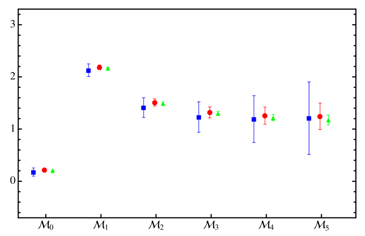
Figure 1: Theoretical moments, Eq. (8), (multiplied by $10^{n}\,\mbox{GeV}^{2n}$) for the charm quark using $\hat{m}_{c}(\hat{m}_{c})=1.272$ GeV at different orders of $\hat{\alpha}_{s}$. Blue squares show results of Eq. (8) up to ${\cal O}(\hat{\alpha}_{s})$, red circles up to ${\cal O}(\hat{\alpha}_{s}^{2})$, and green triangles up to ${\cal O}(\hat{\alpha}_{s}^{3})$. The error bars show the truncation errors given in Eq. (12) at the given order.

$\Delta\hat{m}_{c}(\hat{m}_{c})$	$({\cal M}_{0},{\cal M}_{1})$	$({\cal M}_{0},{\cal M}_{2})$	$({\cal M}_{0},{\cal M}_{3})$	$({\cal M}_{0},{\cal M}_{4})$	$({\cal M}_{0},{\cal M}_{5})$
$\hat{m}_{c}(\hat{m}_{c})$	1280.9	1272.4	1269.1	1265.8	1262.2
$\lambda_{3}^{c}$	1.154	1.230	1.262	1.291	1.323
$\lambda_{3}^{c,{\rm exp}}$	1.35(17)	1.34(17)	1.34(17)	1.33(17)	1.32(17)
Resonances	5.8	4.5	3.9	3.3	2.8
Truncation	6.3	5.9	7.2	8.9	10.5
$\lambda_{3}^{c}-\lambda_{3}^{c,{\rm exp}}$	+6.4	+1.5	+0.3	+0.1	+0.1
$\Delta\lambda_{3}^{c,{\rm exp}}$	4.7	1.7	0.7	0.3	0.2
$10^{3}\times\Delta_{G}$	$-0.25\Delta_{G}$	$-0.37\Delta_{G}$	$-0.54\Delta_{G}$	$-0.73\Delta_{G}$	$-0.88\Delta_{G}$
	$(-1.3)$	${\bf(-1.9)}$	$(-2.7)$	$(-3.7)$	$(-4.4)$
Total	$\pm 11.7$	$\pm 8.0$	$\pm 8.7$	$\pm 10.2$	$\pm 11.7$
$10^{3}\times\Delta\hat{\alpha}_{s}(M_{z})$	$+3.6\Delta\hat{\alpha}_{s}$	$+2.6\Delta\hat{\alpha}_{s}$	$+1.6\Delta\hat{\alpha}_{s}$	$+0.6\Delta\hat{\alpha}_{s}$	$-0.4\Delta\hat{\alpha}_{s}$
Electroweak fit	(+5.8)	(+4.2)	(+2.6)	(+1.0)	($-0.6$)
Lattice	(+4.3)	(+3.1)	(+1.9)	(+0.7)	($-0.5$)

Table 6: Values and breakdown of the uncertainties of $\hat{m}_{c}(\hat{m}_{c})$ (in MeV) and $\lambda_{3}^{c}$ determined from different pairs of moments. The line denoted ’Total’ gives the quadratic sum of the errors from $\lambda_{3}^{c}$, the resonances, the gluon condensate and the pQCD truncation. Numerical values for the uncertainties from $\hat{\alpha}_{s}$ and $C_{G}=\langle\frac{\hat{\alpha}_{s}}{\pi}G^{2}\rangle$ (in units of GeV⁴) are shown in separate lines. In the line labeled ’Electroweak fit’ we use $\Delta\hat{\alpha}_{s}(M_{z})=0.0016$ [25], in the last line denoted ’Lattice’, we use $\Delta\hat{\alpha}_{s}(M_{z})=0.0012$ [8]. See Figure 2 for a graphical representation.

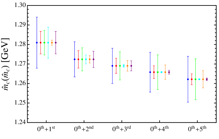
Figure 2: $\hat{m}_{c}(\hat{m}_{c})$ using different combinations of moments and the corresponding uncertianties. Blue represents the full error, red is the one from the resonance region, green from the truncation errors of the theoretical moments, cyan from the error in $\lambda_{3}^{c}$ (which is the symmetrized combination of the shift and the experimental error on $\lambda_{3}^{c}$), orange from the gluon condensate and purple from the uncertainty induced by $\Delta\hat{\alpha}_{s}(M_{Z})=0.0016$. Notice, that all determinations are mutually consistent within our error estimates.

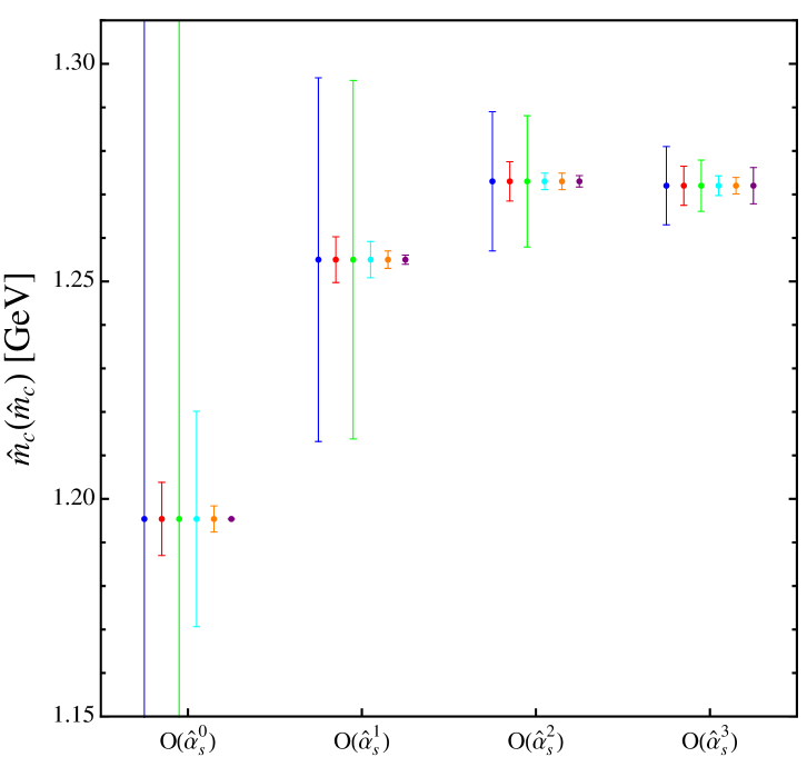
Figure 3: Error budget for $\hat{m}_{c}(\hat{m}_{c})$ determined from the combination of ${\cal M}_{0}$ and ${\cal M}_{2}$ at different orders in $\hat{\alpha}_{s}$. The color coding is as in Figure 2.

In order to determine an error for the continuum contributions (column 3) we proceed in the following way: we compare experimental data with the zeroth moment in the restricted energy range of the threshold region, $2M_{D^{0}}\leq\sqrt{s}\leq 4.8$ GeV, to obtain an experimental value for $\lambda_{3}^{c}$, denoted $\lambda_{3}^{c,{\rm exp}}$ (details will be described below in Section 3). Here we fix $\hat{m}_{c}(\hat{m}_{c})=1.272$ GeV. Then we can also determine an error, $\Delta\lambda_{3}^{c,{\rm exp}}$, from the experimental uncertainty of the data in this threshold region. The shift in the moments resulting from the different values for $\lambda_{3}^{c}$ (either from two moments combined with resonance data only, or from the comparison of the 0th moment with continuum data in the threshold region) turns out to be small. Strictly speaking this shift is a one-sided error, but to be conservative we include it as an additional error in the results of Table 4. Note that non-perturbative effects not included in our expressions for the moments, as for example omitted higher-dimensional condensates, would become visible in the comparison of the values of $\lambda_{3}^{c,{\rm exp}}$ determined from data with $\lambda_{3}^{c}$ obtained from moments. Since we include this difference as a contribution to the uncertainty budget of the charm mass, we do not include an additional uncertainty due to the truncation of the OPE. More details on our determination of $\lambda_{3}^{c,{\rm exp}}$ are given in the next section.

Finally, we assign a truncation error to the theory prediction of the moments. Following the method proposed in Ref. [5] we consider the largest group theoretical factor in the next uncalculated perturbative order as a way to estimate these errors,

$$\Delta{\cal M}_{n}^{(i)}=\pm Q_{q}^{2}N_{C}C_{F}C_{A}^{i-1}\,\left(\frac{\hat{\alpha}_{s}(\hat{m}_{q})}{\pi}\right)^{i}\left(\frac{1}{2\hat{m}_{q}(\hat{m}_{q})}\right)^{2n}\,,$$ (12)

($N_{C}=C_{A}=3$, $C_{F}=4/3$). At order ${\cal O}(\hat{\alpha}_{s}^{4})$, this corresponds to an uncertainty of $\pm 48(\hat{\alpha}_{s}/\pi)^{4}$ for $\hat{C}_{n}^{(4)}$ in Eq. (8). Applying this prescription to the known ${\cal O}(\hat{\alpha}_{s}^{3})$ terms, we observe that the resulting errors are quite conservative: the error estimate from this approach for $\hat{m}_{c}(\hat{m}_{c})$ is more conservative by a factor given in the last column of Table 5 compared to the alternative to base the error estimate on the last known term in the perturbative expansion. We have convinced ourselves that this carries over to the errors for the charm mass: the above prescription is more conservative than the often used alternative approach to vary the renormalization scale within a conventional factor of four.

For the moments with $n>3$ (which, however, will not enter into our final result) taken from Ref. [20] we have to include additional uncertainties specific to the method used to obtain predictions for ${\cal M}_{n}$. These errors are small, but included for completeness. An overview of our theory errors for the moments up to $n=5$ is shown in Figure 1.

The charm mass and the continuum parameter $\lambda_{3}^{c}$ can, in principle, be determined from any combination of two moments. The zeroth moment, however, provides the highest sensitivity. The results for combinations of the zeroth with one higher moment are summarized in Table 6, including the breakdown of the uncertainties due to their different sources. We include the difference between the two possibilities to determine $\lambda_{3}^{c}$ as described above as an estimate of the error due to the method, in particular the truncation of the OPE. In Figure 3 we also show the error budget at different orders of $\hat{\alpha}_{s}$ as obtained from the combination of the moments ${\cal M}_{0}$ and ${\cal M}_{2}$. It is remarkable that the parametric uncertainty due to the input value of $\hat{\alpha}_{s}(M_{Z})$ increases at the last step from $O(\hat{\alpha}_{s}^{2})$ to $O(\hat{\alpha}_{s}^{3})$ (see the last, purple error bars), while the central value for $\hat{m}_{c}(\hat{m}_{c})$ remains stable. A closer look at the underlying formulae reveals that this is due to the bad convergence of the right-hand side of Eq. (6). It is therefore unlikely that knowledge of the next terms in the perturbative series will lead to a reduction of the error on the charm mass. Our final result for the charm quark mass,

$$\hat{m}_{c}(\hat{m}_{c})=(1272+2616\Delta\hat{\alpha}_{s}\pm 8)~{}{\rm MeV},$$ (13)

is based on $({\cal M}_{0},{\cal M}_{2})$ where we explicitly exhibit its dependence on $\hat{\alpha}_{s}$ relative to our adopted central value, i.e., $\Delta\hat{\alpha}_{s}=\hat{\alpha}_{s}(M_{z})-0.1182$.

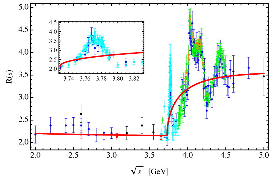
Figure 4: Data for the ratio $R(s)$ for $e^{+}e^{-}\rightarrow$ hadrons in the charm threshold region: Crystal Ball CB86 (green) [27]; BES00, 02, 06, 09 (black, blue, cyan, and red) [28, 29, 30, 31], and CLEO09 (orange) [32]. The full (red) curve is our parametrization of $R_{c}^{\rm cont}(s)$ with $\lambda_{3}^{c}=1.23$ and $\hat{m}_{c}(\hat{m}_{c})=1.272$ GeV. The inner plot is a zoom into the energy range $2M_{D^{0}}\leq\sqrt{s}\leq 3.83$ GeV.

3 Continuum data

Our final result for the charm quark mass given above in Eq. (13) is obtained from an analysis of sum rule moments without using experimental data from the continuum region. Instead, the continuum is described by the parameter $\lambda_{3}^{c}$, and determined simultaneously with $\hat{m}_{c}$ within our formalism. In this section we show that Eq. (5) indeed reproduces the experimental moments well (even though our ansatz must obviously fail to describe the underlying cross section data locally).

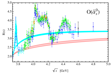
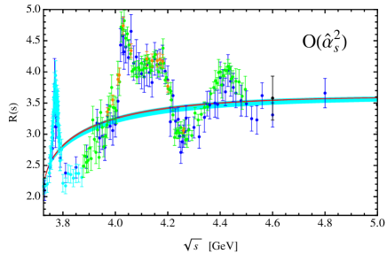
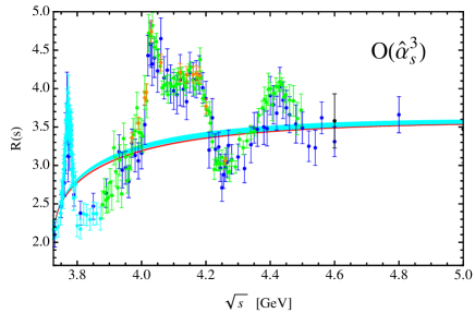
Figure 5: Same as Figure 4 at different orders of $\hat{\alpha}_{s}$. For the full (red) curve we have used $\lambda_{3}^{c}$ determined from the pair of moments ${\cal M}_{0}$ and ${\cal M}_{2}$ at the respective order indicated in the plots with errors as described in the text, while for the blue band we have used $\lambda_{3}^{c,{\rm exp}}$ determined from data and their uncertainties at each order in $\hat{\alpha}_{s}$.

In order to do so, we have to add the background from light-quark contributions [6, 33, 34, 22], $R_{\rm background}(s)=R_{\rm uds}(s)+R_{\rm uds(cb)}(s)+R_{\rm singlet}(s)+R_{\rm QED}(s)$ to our model for the charm continuum. The first part, $R_{\rm uds}(s)$, is given by Eq. (2) with $n_{q}=3$. Contributions from virtual or secondary heavy quarks, $R_{\rm uds(cb)}(s)$, appear first at ${\cal O}(\hat{\alpha}_{s}^{2})$ and are known up to ${\cal O}(\hat{\alpha}_{s}^{3})$ in approximate form [33]. In addition, at order ${\cal O}(\hat{\alpha}_{s}^{3})$ one has to take into account the singlet contribution $R_{\rm singlet}(s)$ [33] which is found to be numerically small, $-0.55(\hat{\alpha}_{s}/\pi)^{3}$ [22], but included for completeness. Finally, also corrections to QED have been taken into account through $R_{\rm QED}(s)$ [6].

In Figure 4 we show the resulting $R$ ratio, $R(s)=R_{c}^{\rm cont}(s)+R_{\rm background}(s)$, compared with experimental $e^{+}e^{-}$ annihilation data for final state hadrons. The data are compiled from Crystal Ball [27], BES [28, 29, 30, 31], and CLEO [32]. The inset zooms into the region above threshold in the energy range of the $\Psi(3770)$ resonance, $2M_{D^{0}}\leq\sqrt{s}\leq 3.83$ GeV, with data points from BES [29, 30]. The full red curve in this figure is obtained from our parametrization of $R_{c}^{\rm cont}(s)$ in Eq. (5), with $\lambda_{3}^{c}=1.23$ and $\hat{m}_{c}(\hat{m}_{c})$ in Eq. (13).

Collab.	$n$	[$2M_{D^{0}},3.872$]	$[3.872,3.97]$	$[3.97,4.26]$	$[4.26,4.496]$	$[4.496,4.8]$
CB86	$0$	—	0.0339(22)(24)	0.2456(25)(172)	0.1543(27)(108)	—
	$1$	—	0.0220(14)(15)	0.1459(16)(102)	0.0801(14)(56)	—
	$2$	—	0.0143(9)(10)	0.0868 (9)(61)	0.0416(7)(29)	—
BES02	$0$	0.0334(24)(17)	0.0362(29)(18)	0.2362(41)(118)	0.1399(38)(70)	0.1705(63)(85)
	$1$	0.0232(17)(12)	0.0235(19)(12)	0.1401(24)(70)	0.0726(20)(36)	0.0788(30)(39)
	$2$	0.0161(12)(8)	0.0152(13)(8)	0.0832(15)(42)	0.0378(10)(19)	0.0365(14)(18)
BES06	$0$	0.0311(16)(15)	—	—	—	—
	$1$	0.0217(11)(11)	—	—	—	—
	$2$	0.0151(8)(7)	—	—	—	—
CLEO09	$0$	—	—	0.2591(22)(52)	—	—
	$1$	—	—	0.1539(13)(31)	—	—
	$2$	—	—	0.0915(8)(18)	—	—
Total	$0$	0.0319(14)(11)	0.0350(18)(15)	0.2545(18)(46)	0.1448(27)(59)	0.1705(63)(85)
	$1$	0.0222(9)(8)	0.0227(12)(10)	0.1511(11)(27)	0.0752(14)(31)	0.0788(30)(39)
	$2$	0.0155(6)(6)	0.0147(8)(6)	0.0899(6)(16)	0.0391(7)(16)	0.0365(14)(18)

Table 7: Contributions to the charm moments ($\times 10^{n}\,\mbox{GeV}^{2n}$) from different energy intervals (given in GeV) and experimental collaborations (CB86 [27], BES02 [29], BES06 [30], CLEO09 [32]). The first errors are statistical and the second systematic. The last lines show the averaged results.

As described in the previous section, we can use data directly to obtain an experimental value $\lambda_{3}^{c,{\rm exp}}$. A comparison of our ansatz Eq. (5) using either this experimental parameter or the one determined via pairs of moments as explained above is shown in Figure 5. Here we compare the resulting parametrizations of the charm continuum with data based on a determination of either $\lambda_{3}^{c}$ or $\lambda_{3}^{c,{\rm exp}}$ performed at different orders of pQCD. The red bands in Figure 5 use $\lambda_{3}^{c}$ and $\hat{m}_{c}(\hat{m}_{c})$ obtained at each order in $\hat{\alpha}_{s}$ while the blue bands use the same value for $\hat{m}_{c}(\hat{m}_{c})$, but $\lambda_{3}^{c,{\rm exp}}$ instead, obtained using Eq. (16) at each order in $\hat{\alpha}_{s}$. We observe that the differences when going from $O(\hat{\alpha}_{s})$ to $O(\hat{\alpha}_{s}^{2})$ and from $O(\hat{\alpha}_{s}^{2})$ to $O(\hat{\alpha}_{s}^{3})$ are of very similar size. This can be traced back to the slow convergence of the coefficients in $\lambda_{1}^{c}(s)$ of Eq. (2). It is interesting to note that this does not lead to large changes in the values of $\hat{m}_{c}(\hat{m}_{c})$ as is evident from Figure 3. Note that we do not assign an extra error to $R_{\rm background}(s)$ since any uncertainty in this quantity is relegated to $\Delta\lambda_{3}^{c,{\rm exp}}$.

We now have a closer look at the determination of moments from data in the energy range $2M_{D^{0}}\leq\sqrt{s}\leq 4.8$ GeV. After light-quark background subtraction, we calculate the contributions to the moments in the considered energy range by numerical integration over the data. In Table 7 we show the results for the zeroth, first, and second moments with data taken from Refs. [27, 29, 30, 32]. We display the separate contributions from each individual collaboration split into five different energy intervals. These intervals have been chosen in such a way that none of the published data had to be split up into smaller segments than originally reported by the collaborations. The first errors are statistical and the second systematic. The statistical errors are uncorrelated. The systematic errors are taken uncorrelated among different collaborations, but completely correlated for data from the same collaboration. The last part in Table 7 (labelled ’Total’) shows the average of the contributions from the different collaborations in each energy interval. The averaging procedure follows Ref. [35]. This prescription takes the relative weights of statistical and systematic errors from each collaboration into account. The breakdown of the total error $\Delta_{\rm tot}$ into statistical ($\Delta_{\rm stat}$) and systematic ($\Delta_{\rm sys}$) contributions can then be calculated in terms of the statistical ($\Delta{\rm C}^{i}_{\rm stat}$) and systematic ($\Delta{\rm C}^{i}_{\rm sys}$) errors of collaboration $i$ contributing to the given interval as [35]

$$(\Delta_{\rm stat})^{2} = \sum_{i}(\Delta{\rm C}^{i}_{\rm stat})^{2}\left(\frac{\Delta_{\rm tot}}{\sqrt{(\Delta{\rm C}^{i}_{\rm stat})^{2}+(\Delta{\rm C}^{i}_{\rm sys})^{2}}}\right)^{4},$$ (14)

$$(\Delta_{\rm sys})^{2} = \sum_{i}(\Delta{\rm C}^{i}_{\rm sys})^{2}\left(\frac{\Delta_{\rm tot}}{\sqrt{(\Delta{\rm C}^{i}_{\rm stat})^{2}+(\Delta{\rm C}^{i}_{\rm sys})^{2}}}\right)^{4}.$$ (15)

$n$	Data	$\lambda^{c}_{3}=1.34(17)$	$\lambda^{c}_{3}=1.23$
0	0.6367(195)	0.6367(195)	0.6239
1	0.3500(102)	0.3509(111)	0.3436
2	0.1957(54)	0.1970(65)	0.1928
3	0.1111(29)	0.1127(38)	0.1102
4	0.0641(16)	0.0657(23)	0.0642
5	0.0375(9)	0.0389(14)	0.0380

Table 8: Contributions to the charm moments ($\times 10^{n}\,\mbox{GeV}^{2n}$) from the energy range $2M_{D^{0}}\leq\sqrt{s}\leq 4.8$ GeV. For the results in the column labeled ’Data’, light-quark contributions have been subtracted using the pQCD prediction at order ${\cal O}(\hat{\alpha}_{s}^{3})$. These entries are obtained from the data displayed in Table 7, taking into account the correlation of systematic errors within each experiment. The third column uses $\hat{m}_{c}=1.272\,{\rm GeV}$ and $\lambda_{3}^{c,{\rm exp}}$ determined by the zeroth experimental moment (see text for details). The last column shows the theoretical prediction for the moments using $\hat{m}_{c}=1.272\,{\rm GeV}$ and $\lambda^{c}_{3}=1.23$, not including condensates.

The final averaged result for the energy range between $2M_{D^{0}}$ and $\sqrt{s}=4.8$ GeV is given in Table 8 up to the fifth moment. The errors shown there are the combined statistical and systematic ones. The third column shows the theoretical moments, again restricted to the region $2M_{D^{0}}\leq\sqrt{s}\leq 4.8$ GeV, using $\hat{m}_{c}=1.272$ GeV as input, and choosing the parameter $\lambda_{3}^{c}$ to match the zeroth experimental moment,

$$\int_{(2M_{D^{0}})^{2}}^{(4.8{\rm\,GeV})^{2}}\frac{{\rm d}s}{s}R_{c}^{\rm cont}(s)\Big{|}_{\hat{m}_{c}=1.272\,{\rm GeV}}={\cal M}_{0}^{\rm Data}=0.6367(195)$$ (16)

which gives the value $\lambda_{3}^{c,{\rm exp}}=1.34(17)$. Finally, the fourth column shows the theoretical calculation of the moments in the threshold region for $\hat{m}_{c}=1.272$ GeV and using the previous value $\lambda_{3}^{c}=1.23$ found above. The agreement between these three columns is remarkable and shows that the data in this restricted energy range is well described by $R_{c}^{\rm cont}(s)$ in Eq. (5).

In the analysis of the previous section only the two narrow resonances below the heavy-quark threshold, i.e., the $J/\Psi$ and $\Psi(2S)$, have been treated separately, while the other charmonium states were included in the continuum. We now study the effect of treating also the $\Psi(3770)$ resonance separately and include it based on the narrow width approximation.

$n$	Data	$\Psi(3770)\big{|}_{\rm BW}$	$\lambda^{c}_{3}=1.23$
0	0.0268(14)	0.0291(20)	0.0339
1	0.0188(10)	0.0204(14)	0.0236
2	0.0132(7)	0.0143(10)	0.0165
3	0.0092(5)	0.0101(7)	0.0115
4	0.0065(3)	0.0071(5)	0.0080
5	0.0045(2)	0.0050(3)	0.0056

Table 9: Contributions to the charm moments ($\times 10^{n}\,\mbox{GeV}^{2n}$) from the energy range $2M_{D^{0}}\leq\sqrt{s}\leq 3.83$ GeV. For the results in the column labeled ’Data’, light-quark contributions have been subtracted using the pQCD prediction at order ${\cal O}(\hat{\alpha}_{s}^{3})$. ’BW’ refers to the Breit-Wigner expression in Eq. (17). The last column shows the theoretical prediction for the moment using $\hat{m}_{c}=1.272\,{\rm GeV}$ and $\lambda^{c}_{3}=1.23$, not including condensates.

Table 9 shows a comparison of charm moments in the closer vicinity of the $\Psi(3770)$ resonance. In the column labeled ’Data’, the moments have been calculated as above, i.e. directly from data, but now restricted to the energy range $2M_{D^{0}}\leq\sqrt{s}\leq 3.83$ GeV (see the inner plot of Figure 4) again after subtraction of the light-quark contribution. The upper limit of this energy interval is chosen to cover the $\Psi(3770)$ resonance completely. In the third column (labeled $\Psi(3770)$) we display results obtained assuming that the resonance is not narrow enough to justify using Eq. (4). Instead, we use the full Breit-Wigner form,

$$R^{\rm\Psi(3770)}_{\rm BW}=\frac{9\Gamma^{e}_{R}\Gamma_{R}}{\alpha_{\rm em}^{2}(M_{R}^{2})}\,\frac{M_{R}^{2}}{(s-M_{R}^{2})^{2}+\Gamma_{R}^{2}M_{R}^{2}}$$ (17)

with $M_{\Psi(3770)}=3.773$ GeV, $\Gamma_{\Psi(3770)}^{e}=0.262(18)$ keV, and $\Gamma_{R}=27.2\pm 1.0$ MeV for the total width of the $\Psi(3770)$ [8]. Even though one can not assume that the $\Psi(3770)$ resonance saturates the charm cross section in this narrow energy range, a Breit-Wigner description agrees with the prediction based on Eq. (5) when $R_{c}^{\rm cont}(s)$ is used with $\lambda_{3}^{c}=1.23$.

Another way to estimate the impact of the $\Psi(3770)$ region on the charm quark mass is to include the $\Psi(3770)$ into our parameterization for $R_{c}^{\rm Res}(s)$ as a $\delta$-function (4) and re-evaluate $\hat{m}_{c}(\hat{m}_{c})$ and $\lambda^{c}_{3}$ using the pair of moments $({\cal M}_{0},{\cal M}_{2})$. We find shifts of $\Delta\hat{m}_{c}(\hat{m}_{c})=-2.4$ MeV and $\Delta\lambda^{c}_{3}=-0.12$. This procedure adds more weight at lower $\sqrt{s}$; therefore the 2nd moment will increase relative to the 0th moment. As a compensation, the charm mass will decrease. The uncertainties associated with the $\Psi(3770)$ resonance parameters are negligible.

$n$	Data	$\lambda^{c}_{3}=1.15(16)$	$\lambda^{c}_{3}=1.23$
0	0.6149(189)	0.6149(189)	0.6239
1	0.3378(98)	0.3385(108)	0.3436
2	0.1886(52)	0.1898(63)	0.1928
3	0.1070(28)	0.1085(37)	0.1102
4	0.0616(16)	0.0631(22)	0.0642
5	0.0360(9)	0.0374(14)	0.0380

Table 10: Contributions to the charm moments ($\times 10^{n}\,\mbox{GeV}^{2n}$) from the energy range $2M_{D^{0}}\leq\sqrt{s}\leq 4.8$ GeV evaluated after taking into account a $2\,\%$ shift of the normalization of the pQCD prediction to fit the data, to be compared with Table 8. In this case we obtained $\hat{m}_{c}(\hat{m}_{c})=1.272$ GeV and $\lambda^{c}_{3}=1.15(16)$ after matching with the zeroth experimental moment.

One may also raise the question whether the specific prescription for the subtraction of the light-quark background in the charm sub-threshold region should be modified, or whether an additional error should be assigned to this prescription. To check the impact of this effect, we have fitted the pQCD prediction including a free normalization factor to the data between $\sqrt{s}=2$ GeV and $2M_{D}$. We found a normalization factor of $1.02\pm 0.01$ and the moments changed to the values given in Table 10. The charm mass is shifted by less than 1 MeV if this modified light-quark subtraction is used instead of the prescription described above.

4 Alternative fits

The approach described in Section 2 requires to make a choice of a pair of moments from which to determine a value for the charm mass. The results displayed in Table 6 (see the line labelled ’Total’) show that the pair $({\cal M}_{0},{\cal M}_{2})$ leads to the smallest error (not taking into account the uncertainty from $\hat{\alpha}_{s}$). A more careful examination reveals that different sources of the errors contribute with different weights. While the pair $({\cal M}_{0},{\cal M}_{1})$ is the least sensitive to the gluon condensate and most strongly affected by the uncertainty of the experimental data from the continuum region, the pair $({\cal M}_{0},{\cal M}_{3})$ has little sensitivity to the continuum data and is more strongly affected by the truncation of the OPE. In this section we investigate the possibility to perform a fit using also more than two moments. In addition, the approach that we discuss now will allow us to take into account uncertainties on the parameters entering the moments in a more systematic way. This will confirm the robustness of our main result in Eq. (13).

	Constraints	$({\cal M}_{0},{\cal M}_{1},{\cal M}_{2})_{\rho}$	${\cal M}_{0},~{}({\cal M}_{1},{\cal M}_{2})_{\rho}$	${\cal M}_{0},~{}({\cal M}_{1},{\cal M}_{2},{\cal M}_{3})_{\rho}$
$\rho$		$-0.06$	$-0.05$	0.32
$\hat{m}_{c}(\hat{m}_{c})$ [GeV]		$1.275(8)$	$1.275(8)$	$1.271(7)$
$\lambda_{3}^{c}$		$1.19(8)$	$1.19(8)$	$1.19(7)$
$\Gamma^{e}_{J/\Psi}$ [keV]	$5.55(14)$	$5.57(14)$	$5.57(14)$	$5.59(14)$
$\Gamma^{e}_{\Psi(2S)}$ [keV]	$2.36(4)$	$2.36(4)$	$2.36(4)$	$2.36(4)$
$C_{G}$ [GeV4]	$0.005(5)$	$0.005(5)$	$0.005(5)$	$0.004(5)$
$\hat{\alpha}_{s}(M_{z})$	$0.1182(16)$	$0.1178(15)$	$0.1178(15)$	$0.1173(15)$

Table 11: Fit results using the first three (four) moments with different scenarios for the correlation between the moments (see text).

We define a $\chi^{2}$-function by

$$\chi^{2}=\frac{1}{2}\sum_{n,m}\left({\cal M}_{n}-{\cal M}_{n}^{\rm pQCD}\right)\left({\cal C}^{-1}\right)^{nm}\left({\cal M}_{m}-{\cal M}_{m}^{\rm pQCD}\right)+\chi^{2}_{c}$$ (18)

where the ${\cal M}_{n}$ are the sum rule expressions for the moments defined in Eq. (2) for $n>0$, and Eq. (6) multiplyed by $3Q_{c}^{2}$ for $n=0$. The corresponding predictions from perturbative QCD, ${\cal M}_{n}^{\rm pQCD}$, were defined in Eq. (8). We will consider different fit scenarios where we include different sets of moments in the sum of Eq. (18). The coefficients $\left({\cal C}^{-1}\right)^{nm}$ are the elements of a correlation matrix which we choose as

$${\cal C}=\frac{1}{2}\sum_{n,m}\rho^{|n-m|}\Delta{\cal M}_{n}^{(3)}\Delta{\cal M}_{m}^{(3)}$$ (19)

with the truncation error $\Delta{\cal M}_{m}^{(3)}$ defined in Eq. (12). The factor $\rho^{|n-m|}$ serves as an ansatz to include correlations between different moments, where $\rho$ itself is a free parameter. In addition, we will also consider cases with vanishing correlations. In particular, the correlation between the zeroth and the other moments may be much smaller than the correlations between the higher moments (especially adjacent ones). The term $\chi^{2}_{c}$ in Eq. (18) imposes constraints on the variation of parameters like the electronic widths in Table 1, the strong coupling constant, $\hat{\alpha}_{s}(M_{z})^{\rm exp}=0.1182\pm 0.0016$ [8], and the gluon condensate, $C_{G}^{\rm exp}=0.005\pm 0.005$ GeV⁴ [24],

$$\chi^{2}_{c}=\left[\frac{\Gamma^{e}_{J/\Psi}-\Gamma^{e,{\rm exp}}_{J/\Psi}}{\Delta\Gamma^{e}_{J/\Psi}}\right]^{2}+\left[\frac{\Gamma^{e}_{\Psi(2S)}-\Gamma^{e,{\rm exp}}_{\Psi(2S)}}{\Delta\Gamma^{e}_{\Psi(2S)}}\right]^{2}+\left[\frac{\hat{\alpha}_{s}(M_{z})-\hat{\alpha}_{s}(M_{z})^{\rm exp}}{\Delta\hat{\alpha}_{s}(M_{z})}\right]^{2}+\left[\frac{C_{G}-C_{G}^{\rm exp}}{\Delta_{G}}\right]^{2}.$$

Thus, $\chi^{2}$ is a function of six parameters, $\hat{m}_{c}(\hat{m}_{c})$, $\lambda_{3}^{c}$ and $\hat{\alpha}_{s}$ for the continuum part of the moments, the electronic widths $\Gamma^{e}_{J/\Psi}$ and $\Gamma^{e}_{\Psi(2S)}$ for the resonance contributions, and $C_{G}$. In addition there is the correlation parameter $\rho$.

	${\cal M}_{0},~{}{\cal M}_{1}$	${\cal M}_{0},~{}{\cal M}_{2}$	${\cal M}_{0},~{}{\cal M}_{3}$
$\hat{m}_{c}(\hat{m}_{c})$ [GeV]	$1.281(9)$	$1.272(7)$	$1.269(5)$
$\lambda_{3}^{c}$	$1.15(5)$	$1.23(6)$	$1.26(8)$

Table 12: Fit results using pairs of moments without correlation.

We now determine all or a subset of the parameters by minimzing $\chi^{2}$. First, we observe that without correlations between the moments, the minimal $\chi^{2}$ is small. This is likely an indication that the theoretical moments are indeed correlated. Taking into account correlations as described above, we now determine the correlation parameter $\rho$ from the condition that $\chi^{2}_{\rm min}$ be equal to the number of degrees of freedom for each considered fit scenario. Then we determine the allowed parameter ranges by solving the equation $\chi^{2}=\chi^{2}_{\rm min}+1$.

In Table 11 we collect the results of three typical fit scenarios based on the first three (four) moments. Columns three, four and five are results of 6-parameter fits. In the first case (column 3) we assume that all three moments are correlated as described above. In the second case (column 4) we assume that only the first and the second moments are correlated. For the results in column 5 we have also included the moment ${\cal M}_{3}$. In this case the uncertainty is slightly smaller, but we have more confidence in lower moments which are less sensitive to the condensates. Moreover, in this scenario the correlation is larger. The errors are obtained by projecting the contour $\chi^{2}=\chi^{2}_{\rm min}+1$ onto each of the six parameters considered. We observe that the results for the charm mass as well as for the continuum parameter $\lambda_{3}^{c}$ are stable. The other four parameters are shifted away from their experimental values only slightly and stay well within their uncertainties. We have performed additional fits in modified scenarios, e.g., using the first three and four moments without correlations. We observe only small shifts in the fitted charm mass of not more than 4 MeV, which is well within our quoted uncertainty. Also fits with only two moments are stable and the results for $\hat{m}_{c}$ and $\lambda_{3}^{c}$ agree within errors. A few typical examples are shown in Table 12 where no correlation is assumed.

	$\Delta\hat{m}_{c}(\hat{m}_{c})[\mbox{MeV}]$	$\Delta\hat{m}_{c}(\hat{m}_{c})[\mbox{MeV}]$
Central value	1274.5	1272.4
$\Delta\Gamma^{e}_{J/\Psi}$	5.9	4.5
$\Delta\Gamma^{e}_{\Psi(2S)}$	1.4	0.4
Truncation	$-$	5.9
$\Delta\lambda_{3}^{c}$	3.0	2.3
Condensates	1.1	1.9
$\Delta\hat{\alpha}_{s}(M_{Z})$	5.4	4.2
Total	8.7	9.0

Table 13: Error budget for the fit scenario ${\cal M}_{0},~{}({\cal M}_{1},{\cal M}_{2})_{\rho}$ from one-parameter fits for the parameter displayed in each line and using the other parameters fixed at their values given in the last column of Table 11. The last column compares this with our main result determined from the pair $({\cal M}_{0},{\cal M}_{2})$ in Table 6.

Table 13 contains the error budget for the uncertainty of the charm mass in the fit scenario using the moments for $n=0$, 1, and 2 with a correlation between ${\cal M}_{1}$ and ${\cal M}_{2}$. The errors are from one-parameter fits with all other parameters fixed at their best fit values, given in the fourth column of Table 11.

5 Comparison with previous work

Our result agrees within errors with the previous analysis [5] where $\hat{m}_{c}(\hat{m}_{c})=1.289^{+0.040}_{-0.045}$ GeV was found. We traced the moderate numerical difference to the following individual shifts:

• The resonance parameters have been updated in recent years. In particular, the value of $\Gamma^{e}_{J/\Psi}$ changed from $5.26(37)$ keV to $5.55(14)$ keV. The larger electronic widths increase the resonance contribution to the higher moments more than to the zeroth moment. As a consequence of the new values of $\Gamma^{e}_{R}$ the charm quark mass is shifted by $-12$ MeV.

• Both the central value and the uncertainty of $\hat{\alpha}_{s}(M_{z})$ have changed. In Ref. [5], $\hat{\alpha}_{s}(M_{z})=0.1221$ was used, while in the current work we use $\hat{\alpha}_{s}(M_{z})=0.1182$. For $\hat{m}_{c}(\hat{m}_{c})$ this leads to a shift of $-10$ MeV.

• In the current work, we use a non-zero central value for the contribution from the gluon condensate. $C_{G}=0.005$ GeV⁴ with $\hat{\alpha}_{s}(M_{z})=0.1221$ induces a shift of the charm quark mass of $-2$ MeV.

• Terms proportional to $\pi^{2}$ (i.e., $\zeta(2)$) in the definition of $\lambda_{1}^{c}(s)$ in [5] are in fact not present. Correcting this leads to a shift of $+3$ MeV for $\hat{m}_{c}(\hat{m}_{c})$.

• Progress in theoretical calculations of higher-order terms allows us to include effects of ${\cal O}(\hat{\alpha}_{s}^{3})$ in the perturbative coefficients of the moments, in the definition of $\lambda_{1}^{c}(s)$, and in the running of $\hat{\alpha}_{s}$. The combined effect of all ${\cal O}(\hat{\alpha}_{s}^{3})$ terms induces a shift of $+4$ MeV.

• There are far more data for the cross section of $e^{+}e^{-}$ annihilation in the charm threshold region, as well as in the region below the charm threshold. These new data affect only the calibration of the uncertainty, however.

• The inclusion of the singlet piece in the light-quark background subtraction affects the charm mass only at the sub-MeV level.

• Shifts induced by possible variations in $\hat{m}_{b}(\hat{m}_{b})$ amount to at most a few hundred keV.

We summarize the various shifts in the charm quark mass in Table 14 where we also include the corresponding shifts in the continuum parameter $\lambda_{3}^{c}$.

	$\hat{m}_{c}(\hat{m}_{c})$	$\lambda_{3}^{c}$
Ref. [5]	$1289$ MeV	$1.97$
Resonances	$-12$ MeV	$-0.16$
$\hat{\alpha}_{s}(M_{z})$	$-10$ MeV	$-0.23$
Gluon condensate	$-2$ MeV	$+0.02$
No $\pi^{2}$ terms	$+3$ MeV	$-0.36$
${\cal O}(\hat{\alpha}_{s}^{3})$	$+4$ MeV	$-0.57$

Table 14: Comparison between Eq. (13) and the result of Ref. [5] where $\hat{\alpha}_{s}(M_{z})=0.1221$ was used and the breakdown of the different sources of errors. See the text for details.

We also find agreement within errors with other charm quark mass determinations in the literature. The result of Ref. [23], $\hat{m}_{c}(\hat{m}_{c})=1.279(13)$ GeV, obtained from the first moment and using $\hat{\alpha}_{s}(M_{z})=0.1189$ and $C_{G}=0.006(12)$ GeV⁴, agrees very well with the value we find from the pair $({\cal M}_{0},{\cal M}_{1})$ in Table 6. Ref. [37] used the second moment and a modification of the kernel of the sum rule in Eq. (1) to obtain $\hat{m}_{c}(\hat{m}_{c})=1.278(9)$ GeV using as input $\hat{\alpha}_{s}(M_{z})=0.1184(7)$ and $C_{G}=0.01(1)$ GeV⁴. Ref. [38] is based on higher moments extracting $C_{G}=(0.022\pm 0.004)$ GeV⁴ which then yields $\hat{m}_{c}(\hat{m}_{c})=1.261(16)$ GeV. While the charm production cross section is described by a set of six narrow-width resonances, combined with a continuum from perturbative QCD, the difference between Ref. [38] and our result can be explained to a large extent by the different values of the gluon condensate. A more recent analysis [39] extracted the charm quark mass from the first moment sum rule using experimental data from a previous analysis [40]. We can reproduce their final result, $\hat{m}_{c}(\hat{m}_{c})=1.288(20)$ GeV, if we use their input values, $\hat{\alpha}_{s}(M_{z})=0.1184(21)$ and $C_{G}=0.006(12)$ GeV⁴, and the electronic widths of the $\Psi(2S)$ resonance before its recent update. The authors of Ref. [40] have also discussed the $Z$-boson contribution to the QCD moments and found it to be very small. This contribution is neglected in our work.

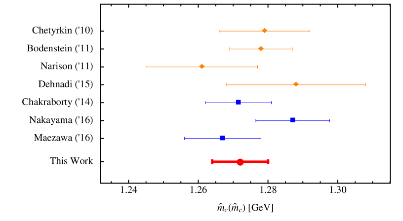
Figure 6: Recent charm quark mass determinations (see text for details and references).

Beyond the phenomenological charm quark mass determinations discussed so far, there are also precise lattice QCD calculations. Ref. [41] reports $\hat{m}_{c}(\hat{m}_{c})=1.2715(95)$ GeV with $\hat{\alpha}_{s}(M_{z})=0.11822(74)$ from a study of pseudoscalar-pseudoscalar correlators. Ref. [42], using Möbius domain-wall fermions to describe both light and charm quarks, obtained the value $\hat{m}_{c}(\hat{m}_{c})=1.2871(106)$ GeV for $\hat{\alpha}_{s}(M_{z})=0.1177(25)$. A value for the gluon condensate was also fitted and found to be compatible with zero. Finally, Ref. [43] used the Highly Improved Staggered Quark action and moments of the pseudsocalar-charmonium correlator, and found $\hat{m}_{c}(\hat{m}_{c})=1.267(11)$ GeV and $\hat{\alpha}_{s}(M_{z})=0.1162(75)$. These results are displayed in Figure 6.

6 Conclusions

We presented a determination of the charm quark mass from QCD sum rules with a careful determination of the uncertainty. We included the zeroth moment in our strategy and exploited the consistency between different moments. The usefulness of the zeroth moment is not its sensitivity to $\hat{m}_{c}$ itself (which is mild), but to the continuum contribution to which it is very sensitive. While the coefficient $A_{3}$ entering the zeroth moment through Eq. (6) is uncomfortably large, we fully account for this by our conservative error estimate in Eq. (12). It is interesting to note, however, that the dispersive calculation of the value of the electromagnetic coupling $\alpha_{\rm em}$ at the $Z$-pole (an essential input into the calculation of the $W$ boson mass, as well as for the electroweak program at LEP and any future $Z$ factory), effectively relies on precisely the zeroth moment. One usually neglects to make any reference to what value of $\hat{m}_{c}$ the charm quark contribution to $\alpha_{\rm em}(M_{Z})$ would correspond to and whether that value is compatible with other determinations. It is this relation that shows poor convergence. Our approach amounts to determining the error on $\hat{m}_{c}$ by demanding compatibility with some higher moment. Our value of $\hat{m}_{c}$ in Eq. (13) can then be used along the lines of Ref. [36], where perturbative QCD was used to directly compute $\alpha_{\rm em}(M_{Z})$ in the $\overline{\rm MS}$ scheme (with $\hat{m}_{c}$ as an external input).

Note, that at this level of accuracy a subtle issue arises: we have implicitly defined $\hat{m}_{c}(\hat{m}_{c})$ as the $\overline{\rm MS}$ mass w.r.t. both QCD and QED, as can be seen e.g. from Eq. (9). Alternatively adopting a hybrid definition, $\hat{m}_{c}(\hat{m}_{c})^{\rm(pole-QED)}$, which assumes the on-shell mass w.r.t. QED so that the QED treatment of quarks mirrors more closely that of leptons, one has,

$$\hat{m}_{c}(\hat{m}_{c})^{\rm(pole-QED)}=\hat{m}_{c}(\hat{m}_{c})\left[1+Q_{c}^{2}\frac{\alpha_{em}(m_{c})}{\pi}+{\cal O}(\alpha_{em}^{2})\right]=(1274+2616\Delta\hat{\alpha}_{s}\pm 8)~{}\mbox{MeV}.$$ (20)

The largest contribution to the total uncertainty in the charm quark mass is the truncation error. Since the coefficients of the perturbative expansion of the moments exhibit no compelling evidence for a convergent behaviour, we consider it unlikely that knowledge of the next terms in the perturbative series will lead to a reduction of the error on the charm mass.

In future work we will apply our approach also to the case of the bottom quark. We believe that we should be able to justify an error estimate for $\hat{m}_{b}(\hat{m}_{b})$ of about 15 MeV. This follows from the fact that our determination of the charm mass scales with the difference between half of the lowest-mass resonance, $M_{J/\Psi}/2$, and the quark mass $\hat{m}_{c}(\hat{m}_{c})$. Our uncertainty of $\Delta\hat{m}_{c}(\hat{m}_{c})=8$ MeV corresponds to $2.9\,\%$ of this difference. Translated to the case of the $b$ quark, using $M_{\Upsilon}=9.460$ GeV and $\hat{m}_{b}(\hat{m}_{b})\sim 4.200$ GeV, this would correspond to 15 MeV.

References

- [1] J. Erler, AIP Conf. Proc. 1701, 020009 (2016) [arXiv:1412.4435 [hep-ph]].
- [2] V. A. Novikov, L. B. Okun, M. A. Shifman, A. I. Vainshtein, M. B. Voloshin and V. I. Zakharov, Phys. Rept. 41, 1 (1978).
- [3] M. A. Shifman, A. I. Vainshtein and V. I. Zakharov, Nucl. Phys. B 147, 385 (1979).
- [4] M. A. Shifman, A. I. Vainshtein and V. I. Zakharov, Nucl. Phys. B 147, 448 (1979).
- [5] J. Erler and M. x. Luo, Phys. Lett. B 558, 125 (2003) [hep-ph/0207114].
- [6] K. G. Chetyrkin, J. H. Kuhn and A. Kwiatkowski, Phys. Rept. 277, 189 (1996) [hep-ph/9503396].
- [7] K. G. Chetyrkin, R. V. Harlander and J. H. Kuhn, Nucl. Phys. B 586, 56 (2000) Erratum: [Nucl. Phys. B 634, 413 (2002)] [hep-ph/0005139].
- [8] K. A. Olive et al. [Particle Data Group], Chin. Phys. C 38, 090001 (2014).
- [9] F. Jegerlehner, http://www-com.physik.hu-berlin.de/~fjeger/.
- [10] K. G. Chetyrkin, J. H. Kuhn and M. Steinhauser, Nucl. Phys. B 482, 213 (1996) [hep-ph/9606230].
- [11] K. G. Chetyrkin, B. A. Kniehl and M. Steinhauser, Nucl. Phys. B 510, 61 (1998) [hep-ph/9708255].
- [12] Y. Kiyo, A. Maier, P. Maierhofer and P. Marquard, Nucl. Phys. B 823, 269 (2009) [arXiv:0907.2120 [hep-ph]].
- [13] A. H. Hoang, V. Mateu and S. Mohammad Zebarjad, Nucl. Phys. B 813, 349 (2009) [arXiv:0807.4173 [hep-ph]].
- [14] K. G. Chetyrkin, J. H. Kuhn and C. Sturm, Eur. Phys. J. C 48, 107 (2006) [hep-ph/0604234].
- [15] R. Boughezal, M. Czakon and T. Schutzmeier, Phys. Rev. D 74, 074006 (2006) [hep-ph/0605023].
- [16] A. Maier, P. Maierhofer and P. Marquard, Phys. Lett. B 669, 88 (2008) [arXiv:0806.3405 [hep-ph]].
- [17] A. Maier, P. Maierhofer, P. Marquard and A. V. Smirnov, Nucl. Phys. B 824, 1 (2010) [arXiv:0907.2117 [hep-ph]].
- [18] K. G. Chetyrkin, J. H. Kuhn and M. Steinhauser, Nucl. Phys. B 505, 40 (1997) [hep-ph/9705254].
- [19] A. Maier, P. Maierhofer and P. Marquard, Nucl. Phys. B 797, 218 (2008) [arXiv:0711.2636 [hep-ph]].
- [20] D. Greynat, P. Masjuan and S. Peris, Phys. Rev. D 85, 054008 (2012) [arXiv:1104.3425 [hep-ph]].
- [21] D. J. Broadhurst, P. A. Baikov, V. A. Ilyin, J. Fleischer, O. V. Tarasov and V. A. Smirnov, Phys. Lett. B 329, 103 (1994) [hep-ph/9403274].
- [22] J. H. Kuhn, M. Steinhauser and C. Sturm, Nucl. Phys. B 778, 192 (2007) [hep-ph/0702103 [HEP-PH]].
- [23] K. Chetyrkin, J. H. Kuhn, A. Maier, P. Maierhofer, P. Marquard, M. Steinhauser and C. Sturm, Theor. Math. Phys. 170, 217 (2012) [arXiv:1010.6157 [hep-ph]].
- [24] C. A. Dominguez, L. A. Hernandez, K. Schilcher and H. Spiesberger, JHEP 1503, 053 (2015) [arXiv:1410.3779 [hep-ph]].
- [25] J. Erler and A. Freitas, Electroweak Model and Constraints on New Physics, in C. Patrignani et al. [Particle Data Group], Chin. Phys. C 40 (2016) 100001.
- [26] K. G. Chetyrkin, J. H. Kuhn and M. Steinhauser, Comput. Phys. Commun. 133, 43 (2000) [hep-ph/0004189].
- [27] A. Osterheld et al., Phys. Rev. D, 1986.
- [28] J. Z. Bai et al. [BES Collaboration], Phys. Rev. Lett. 84, 594 (2000) [hep-ex/9908046].
- [29] J. Z. Bai et al. [BES Collaboration], Phys. Rev. Lett. 88, 101802 (2002) [hep-ex/0102003].
- [30] M. Ablikim et al., Phys. Rev. Lett. 97, 262001 (2006) [hep-ex/0612054].
- [31] M. Ablikim et al. [BES Collaboration], Phys. Lett. B 677, 239 (2009) [arXiv:0903.0900 [hep-ex]].
- [32] D. Cronin-Hennessy et al. [CLEO Collaboration], Phys. Rev. D 80, 072001 (2009) [arXiv:0801.3418 [hep-ex]].
- [33] R. V. Harlander and M. Steinhauser, Comput. Phys. Commun. 153, 244 (2003) [hep-ph/0212294].
- [34] J. H. Kuhn and M. Steinhauser, Nucl. Phys. B 619, 588 (2001) Erratum: [Nucl. Phys. B 640, 415 (2002)] [hep-ph/0109084].
- [35] J. Erler, Eur. Phys. J. C 75, no. 9, 453 (2015) [arXiv:1507.08210 [physics.data-an]].
- [36] J. Erler, Phys. Rev. D 59, 054008 (1999) [hep-ph/9803453].
- [37] S. Bodenstein, J. Bordes, C. A. Dominguez, J. Penarrocha and K. Schilcher, Phys. Rev. D 83, 074014 (2011) [arXiv:1102.3835 [hep-ph]].
- [38] S. Narison, Phys. Lett. B 706, 412 (2012) [arXiv:1105.2922 [hep-ph]].
- [39] B. Dehnadi, A. H. Hoang and V. Mateu, JHEP 1508, 155 (2015) [arXiv:1504.07638 [hep-ph]].
- [40] B. Dehnadi, A. H. Hoang, V. Mateu and S. M. Zebarjad, JHEP 1309, 103 (2013) [arXiv:1102.2264 [hep-ph]].
- [41] B. Chakraborty et al., Phys. Rev. D 91, no. 5, 054508 (2015) [arXiv:1408.4169 [hep-lat]].
- [42] K. Nakayama, B. Fahy and S. Hashimoto, arXiv:1606.01002 [hep-lat].
- [43] Y. Maezawa and P. Petreczky, arXiv:1606.08798 [hep-lat].