Recurrent Switching Linear Dynamical Systems
Scott W. Linderman Andrew C. Miller Ryan P. Adams
Columbia University Harvard University Harvard University and Twitter
David M. Blei Liam Paninski Matthew J. Johnson
Columbia University Columbia University Harvard University
Abstract
Many natural systems, such as neurons firing in the brain or basketball teams traversing a court, give rise to time series data with complex, nonlinear dynamics. We can gain insight into these systems by decomposing the data into segments that are each explained by simpler dynamic units. Building on switching linear dynamical systems (SLDS), we present a new model class that not only discovers these dynamical units, but also explains how their switching behavior depends on observations or continuous latent states. These “recurrent” switching linear dynamical systems provide further insight by discovering the conditions under which each unit is deployed, something that traditional SLDS models fail to do. We leverage recent algorithmic advances in approximate inference to make Bayesian inference in these models easy, fast, and scalable.
1 Introduction
Complex dynamical behaviors can often be broken down into simpler units. A basketball player finds the right court position and starts a pick and roll play. A mouse senses a predator and decides to dart away and hide. A neuron’s voltage first fluctuates around a baseline until a threshold is exceeded; it spikes to peak depolarization, and then returns to baseline. In each of these cases, the switch to a new mode of behavior can depend on the continuous state of the system or on external factors. By discovering these behavioral units and their switching dependencies, we can gain insight into complex data-generating processes.
This paper proposes a class of recurrent state space models that captures these dependencies and a Bayesian inference and learning algorithm that is computationally tractable and scalable to large datasets. We extend switching linear-Gaussian dynamical systems (SLDS) (Ackerson and Fu, 1970; Chang and Athans, 1978; Hamilton, 1990; Ghahramani and Hinton, 1996; Murphy, 1998; Fox et al., 2009) by introducing a class of models in which the discrete switches can depend on the continuous latent state and exogenous inputs through a logistic regression. Previous models including this dependence, like the piecewise affine framework for hybrid dynamical systems (Sontag, 1981), abandon the conditional linear-Gaussian structure in the continuous states and thus greatly complicate inference (Paoletti et al., 2007; Juloski et al., 2005). Our main technical contribution is a new inference algorithm that leverages auxiliary variable methods (Polson, Scott, and Windle, 2013; Linderman, Johnson, and Adams, 2015) to make inference both fast and easy.
The class of models and the corresponding learning and inference algorithms we develop have several advantages for understanding rich time series data. First, these models decompose data into simple segments and attribute segment transitions to changes in latent state or environment; this provides interpretable representations of data dynamics. Second, we fit these models using fast, modular Bayesian inference algorithms; this makes it easy to handle missing data, multiple observation modalities, and hierarchical extensions. Finally, these models are interpretable, readily able to incorporate prior information, and generative; this lets us take advantage of a variety of tools for model validation and checking.
In the following section we provide background on the key models and inference techniques on which our method builds. Next, we introduce the class of recurrent switching state space models, and then explain the main algorithmic contribution that enables fast learning and inference. Finally, we illustrate the method on synthetic data experiments and an application to recordings of professional basketball players.
2 Background
Our model has two main components: switching linear dynamical systems and stick-breaking logistic regression. Here we review these components and fix the notation we will use throughout the paper.
2.1 Switching linear dynamical systems
Switching linear dynamical system models (SLDS) break down complex, nonlinear time series data into sequences of simpler, reused dynamical modes. By fitting an SLDS to data, we not only learn a flexible nonlinear generative model, but also learn to parse data sequences into coherent discrete units.
The generative model is as follows. At each time there is a discrete latent state that following Markovian dynamics,
| (1) |
where is the Markov transition matrix and is its th row. In addition, a continuous latent state follows conditionally linear (or affine) dynamics, where the discrete state determines the linear dynamical system used at time :
| (2) |
for matrices and vectors for . Finally, at each time a linear Gaussian observation is generated from the corresponding latent continuous state,
| (3) |
for , , and . The system parameters comprise the discrete Markov transition matrix and the library of linear dynamical system matrices, which we write as
For simplicity, we will require , , and to be shared among all discrete states in our experiments. In general, equations (2) and (3) can be extended to include linear dependence on exogenous inputs, , as well.
To learn an SLDS using Bayesian inference, we place conjugate Dirichlet priors on each row of the transition matrix and conjugate matrix normal inverse Wishart (MNIW) priors on the linear dynamical system parameters, writing
where , , and denote hyperparameters.
2.2 Stick-breaking logistic regression and Pólya-gamma augmentation
Another component of the recurrent SLDS is a stick-breaking logistic regression, and for efficient block inference updates we leverage a recent Pólya-gamma augmentation strategy (Linderman, Johnson, and Adams, 2015). This augmentation allows certain logistic regression evidence potentials to appear as conditionally Gaussian potentials in an augmented distribution, which enables our fast inference algorithms.
Consider a logistic regression model from regressors to a categorical distribution on the discrete variable , written as
| (4) |
where is a weight matrix and is a bias vector. Unlike the standard multiclass logistic regression, which uses a softmax link function, we instead use a stick-breaking link function , which maps a real vector to a normalized probability vector via the stick-breaking process
for and , where denotes the logistic function. The probability mass function is
where denotes an indicator function that takes value when its argument is true and otherwise.
If we use this regression model as a likelihood with a Gaussian prior density , the posterior density is non-Gaussian and does not admit easy Bayesian updating. However, Linderman, Johnson, and Adams (2015) show how to introduce Pólya-gamma auxiliary variables so that the conditional density becomes Gaussian. In particular, by choosing , we have,
where the mean vector and covariance matrix are determined by
| (5) |
Thus instantiating these auxiliary variables in a Gibbs sampler or variational mean field inference algorithm enables efficient block updates while preserving the same marginal posterior distribution .
3 Recurrent Switching State Space Models
The discrete states in the “classical” SLDS of Section 2.1 are generated via an open loop: the discrete state is a function only of the preceding discrete state , and is independent of the continuous state . That is, if a discrete switch should occur whenever the continuous state enters a particular region of state space, the SLDS will be unable to learn this dependence.
We introduce the recurrent switching linear dynamical system (rSLDS), an extension of the SLDS to model these dependencies directly. Rather than restricting the discrete states to open-loop Markovian dynamics as in Eq. (1), the rSLDS allows the discrete state transition probabilities to depend on additional covariates, and in particular on the preceding continuous latent state. That is, the discrete states of the rSLDS are generated as
| (6) |
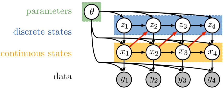
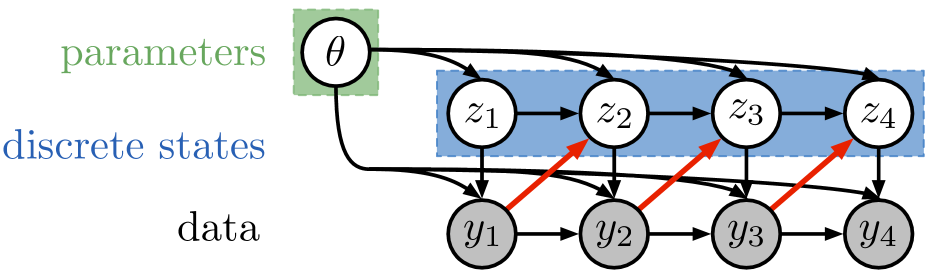
where is a weight matrix that specifies the recurrent dependencies and is a bias that captures the Markov dependence of on . The remainder of the rSLDS generative process follows that of the SLDS from Eqs. (2)-(3). See Figure 2(a) for a graphical model, where the edges representing the new dependencies of the discrete states on the continuous latent states are highlighted in red. As with the standard SLDS, both the discrete and continuous rSLDS dynamics could be extended with linear dependence on exogenous inputs, , as well.
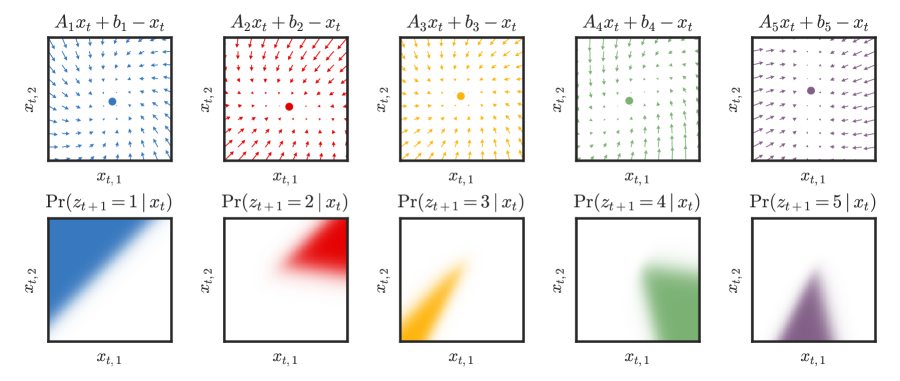
Figure 1 illustrates an rSLDS with discrete states and dimensional continuous states. Each discrete state corresponds to a set of linear dynamics defined by and , shown in the top row. The transition probability, , is a function of the previous states and . We show only the dependence on in the bottom row. Each panel shows the conditional probability, , as a colormap ranging from zero (white) to one (color). Due to the logistic stick breaking, the latent space is iteratively partitioned with linear hyperplanes.
There are several useful special cases of the rSLDS.
Recurrent ARHMM (rAR-HMM)
Just as the autoregressive HMM (AR-HMM) is a special case of the SLDS in which we observe the states directly, we can define an analogous rAR-HMM. See Figure 2(b) for a graphical model, where the edges representing the dependence of the discrete states on the continuous observations are highlighted in red.
Shared rSLDS (rSLDS(s))
Rather than having separate recurrence weights (and hence a separate partition) for each value of , we can share the recurrence weights as,
Recurrence-Only (rSLDS(ro))
There is no dependence on in this model. Instead,
While less flexible, this model is eminently interpretable, easy to visualize, and, as we show in experiments, works well for many dynamical systems. The example in Figure 1 corresponds to this special case.
Standard SLDS
We can recover the standard SLDS with .
Recurrent Sticky SLDS
Rather than allowing the continuous states to govern the entire distribution over next discrete states, may only affect whether or not to stay in the current state. That is,
| (7) |
where is a distribution on states other than the current state. The “stay-or-leave” variable, , depends on the current location.
4 Bayesian Inference
Adding the recurrent dependencies from the latent continuous states to the latent discrete states introduces new inference challenges. While block Gibbs sampling in the standard SLDS can be accomplished with message passing because is conditionally Gaussian given and , the dependence of on renders the recurrent SLDS non-conjugate. To develop a message-passing procedure for the rSLDS, we first review standard SLDS message passing, then show how to leverage a Pólya-gamma augmentation along with message passing to perform efficient Gibbs sampling in the rSLDS. We discuss stochastic variational inference (Hoffman et al., 2013) in the supplementary material.
4.1 Message Passing
First, consider the conditional density of the latent continuous state sequence given all other variables, which is proportional to
| (8) |
where denotes the potential from the conditionally linear-Gaussian dynamics and denotes the evidence potentials. The potentials arise from the new dependencies in the rSLDS and do not appear in the standard SLDS. This factorization corresponds to a chain-structured undirected graphical model with nodes for each time index.
We can sample from this conditional distribution using message passing. The message from time to time , denoted , is computed via
| (9) |
where denotes . If the potentials were all Gaussian, as is the case without the rSLDS potential , this integral could be computed analytically. We pass messages forward once, as in a Kalman filter, and then sample backward. This constructs a joint sample in time. A similar procedure can be used to jointly sample the discrete state sequence, , given the continuous states and parameters. However, this computational strategy for sampling the latent continuous states breaks down when including the non-Gaussian rSLDS potential .
Note that it is straightforward to handle missing data in this formulation; if the observation is omitted, we simply have one fewer potential in our graph.
4.2 Augmentation for non-Gaussian Factors
The challenge presented by the recurrent SLDS is that is not a linear Gaussian factor; rather, it is a categorical distribution whose parameter depends nonlinearly on . Thus, the integral in the message computation (9) is not available in closed form. There are a number of methods of approximating such integrals, like particle filtering (Doucet et al., 2000) or Laplace approximations (Tierney and Kadane, 1986), but here we take an alternative approach using the recently developed Pólya-gamma augmentation scheme (Polson et al., 2013), which renders the model conjugate by introducing an auxiliary variable in such a way that the resulting marginal leaves the original model intact.
According to the stick breaking transformation described in Section 2.2, the non-Gaussian factor is
where is the -th dimension of , as defined in (6). Recall that is linear in . Expanding the definition of the logistic function, we have,
| (10) |
The Pólya-gamma augmentation targets exactly such densities, leveraging the following integral identity:
| (11) |
where and is the density of the Pólya-gamma distribution, , which does not depend on .
Combining (10) and (11), we see that can be written as a marginal of a factor on the augmented space, , where is a vector of auxiliary variables. As a function of , we have
| (12) |
where . Hence,
| (13) |
with and . Again, recall that is a linear function of . Thus, after augmentation, the potential on is effectively Gaussian and the integrals required for message passing can be written analytically. Finally, the auxiliary variables are easily updated as well, since .
4.3 Updating Model Parameters
Given the latent states and observations, the model parameters benefit from simple conjugate updates. The dynamics parameters have conjugate MNIW priors, as do the emission parameters. The recurrence weights are also conjugate under a MNIW prior, given the auxiliary variables . We set the hyperparameters of these priors such that random draws of the dynamics are typically stable and have nearly unit spectral radius in expectation, and we set the mean of the recurrence bias such that states are equiprobable in expectation. We will discuss initialization in the following section.
4.4 Initialization
Given the complexity of these models, it is important to initialize the parameters and latent states with reasonable values. We used the following initialization procedure: (i) use probabilistic PCA or factor analysis to initialize the continuous latent states, , and the observation, , , and ; (ii) fit an AR-HMM to in order to initialize the discrete latent states, , and the dynamics models, ; and then (iii) greedily fit a decision list with logistic regressions at each node in order to determine a permutation of the latent states most amenable to stick breaking. In practice, the last step alleviates the undesirable dependence on ordering that arises from the stick breaking formulation. We discuss this and alternative approaches in more depth in the supplementary material.
With this initialization, the Gibbs sampler refines the parameter and state estimates and explores (at least a mode of) the posterior.
5 Experiments
We demonstrate the potential of recurrent dynamics in a variety of settings. First, we consider a case in which the underlying dynamics truly follow an rSLDS, which illustrates some of the nuances involved in fitting these rich systems. With this experience, we then apply these models to simulated data from a canonical nonlinear dynamical system – the Lorenz attractor – and find that its dynamics are well-approximated by an rSLDS. Moreover, by leveraging the Pólya-gamma augmentation, these nonlinear dynamics can even be recovered from discrete time series with large swaths of missing data, as we show with a Bernoulli-Lorenz model. Finally, we apply these recurrent models to real trajectories on basketball players and discover interpretable, location-dependent behavioral states.
5.1 Synthetic NASCAR®
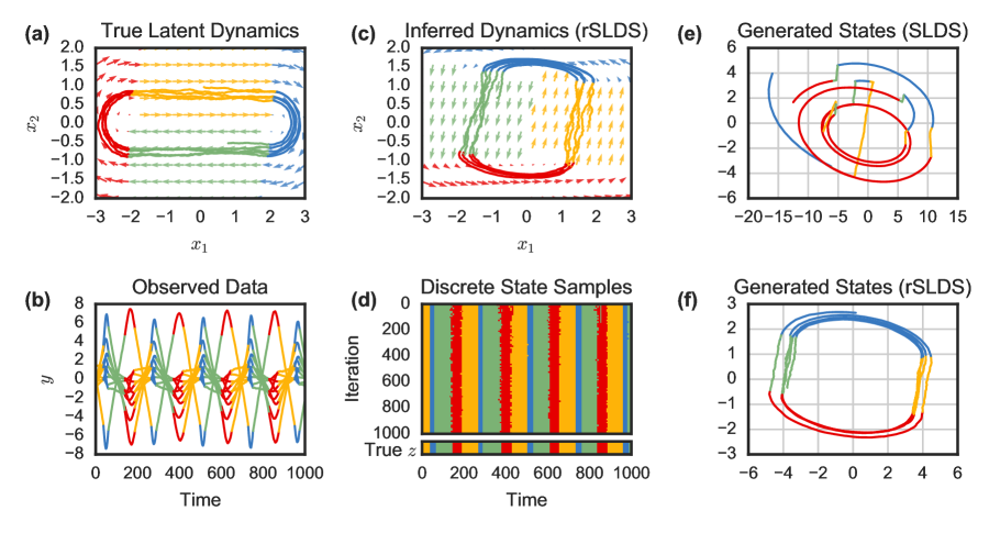
We begin with a toy example in which the true dynamics trace out ovals, like a stock car on a NASCAR® track.111Unlike real NASCAR drivers, these states turn right. There are four discrete states, , that govern the dynamics of a two dimensional continuous latent state, . Fig. 3a shows the dynamics of the most likely state for each point in latent space, along with a sampled trajectory from this system. The observations, are a linear projection of the latent state with additive Gaussian noise. The 10 dimensions of are superimposed in Fig. 3b. We simulated time-steps of data and fit an rSLDS to these data with iterations of Gibbs sampling.
Fig. 3c shows a sample of the inferred latent state and its dynamics. It recovers the four states and a rotated oval track, which is expected since the latent states are non-identifiable up to invertible transformation. Fig. 3d plots the samples of as a function of Gibbs iteration, illustrating the uncertainty near the change-points.
From a decoding perspective, both the SLDS and the rSLDS are capable of discovering the discrete latent states; however, the rSLDS is a much more effective generative model. Whereas the standard SLDS has only a Markov model for the discrete states, and hence generates the geometrically distributed state durations in Fig 3e, the rSLDS leverages the location of the latent state to govern the discrete dynamics and generates the much more realistic, periodic data in Fig. 3f.
5.2 Lorenz Attractor
Switching linear dynamical systems offer a tractable approximation to complicated nonlinear dynamical systems. Indeed, one of the principal motivations for these models is that once they have been fit, we can leverage decades of research on optimal filtering, smoothing, and control for linear systems. However, as we show in the case of the Lorenz attractor, the standard SLDS is often a poor generative model, and hence has difficulty interpolating over missing data. The recurrent SLDS remedies this by connecting discrete and continuous states.
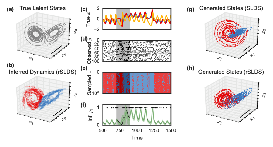
Fig. 4a shows the states of a Lorenz attractor, whose nonlinear dynamics are given by,
| (14) |
Though nonlinear and chaotic, we see that the Lorenz attractor roughly traces out ellipses in two opposing planes. Fig. 4c unrolls these dynamics over time, where the periodic nature and the discrete jumps become clear.
Rather than directly observing the Lorenz states, , we simulate dimensional discrete observations from a generalized linear model,
| (15) |
where is the logistic function. A window of observations is shown in Fig. 4d. Just as we leveraged the Pólya-gamma augmentation to render the continuous latent states conjugate with the multinomial discrete state samples, we again leverage the augmentation scheme to render them conjugate with Bernoulli observations. As a further challenge, we also hold out a slice of data for , identified by a gray mask in the center panels. We provide more details in the supplementary material.
Fitting an rSLDS via the same procedure described above, we find that the model separates these two planes into two distinct states, each with linear, rotational dynamics shown in Fig. 4b. Note that the latent states are only identifiable up to invertible transformation. Comparing Fig. 4e to panel c, we see that the rSLDS samples changes in discrete state at the points of large jumps in the data, but when the observations are masked, there is more uncertainty. This uncertainty in discrete state is propagated to uncertainty in the event probability, , which is shown for the first output dimension in Fig. 4f. The times are shown as dots, and the mean posterior probability is shown with standard deviations. Again, even in the absence of observations, the model is capable of intelligently interpolating, inferring when there should be a discrete change in dynamics.
Finally, as expected, data generated from a standard SLDS fit in the same manner is quite different from the real data. It switches from one state to another independent of the location, resulting in large divergences from the origin. In contrast, the rSLDS states are noisy yet qualitatively similar to those of the true Lorenz attractor.
5.3 Basketball Player Trajectories
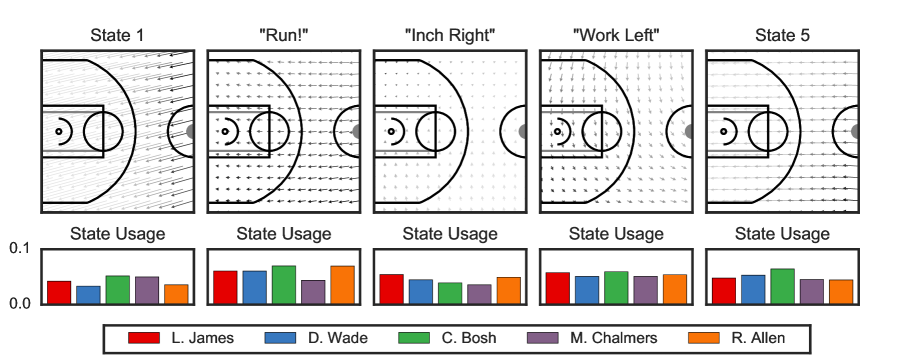
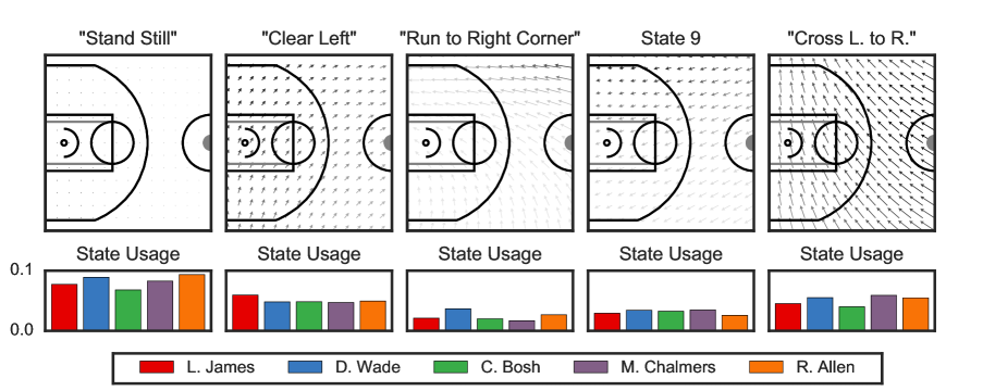
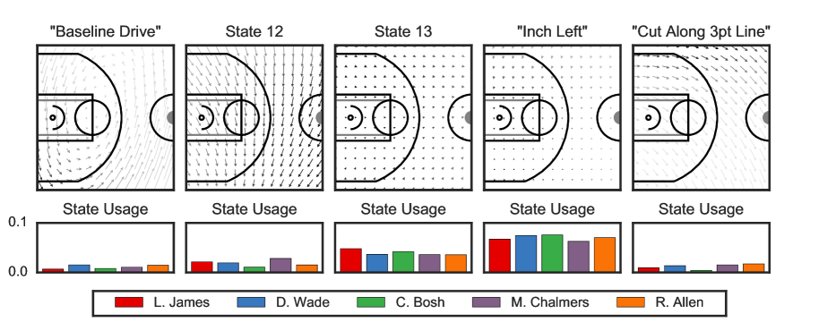
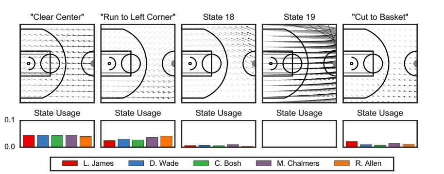
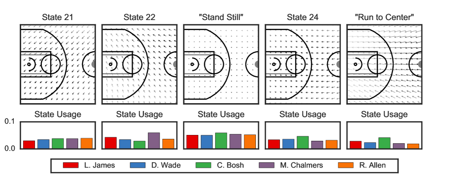
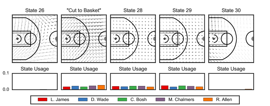
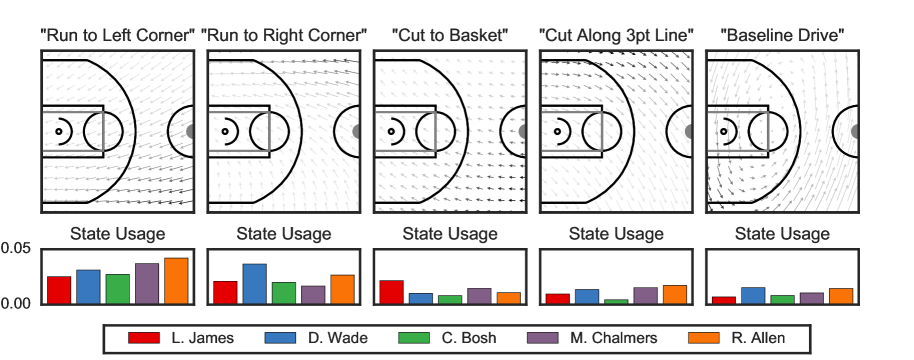
We further illustrate our recurrent models with an application to the trajectories run by five National Basketball Association (NBA) players from the Miami Heat in a game against the Brooklyn Nets on Nov. 1st, 2013. We are given trajectories, , for each player . We treat these trajectories as independent realizations of a “recurrence-only” AR-HMM with a shared set of states. Positions are recorded every 40ms; combining the five players yields 256,103 time steps in total. We use our rAR-HMM to discover discrete dynamical states as well as the court locations in which those states are most likely to be deployed. We fit the model with 200 iteration of Gibbs sampling, initialized with a draw from the prior.
The dynamics of five of the discovered states are shown in Fig. 5 (top), along with the names we have assigned them. Below, we show the frequency with which each player uses the states under the posterior distribution. First, we notice lateral symmetry; some players drive to the left corner whereas others drive to the right. Anecdotally, Ray Allen is known to shoot more from the left corner, which agrees with the state usage here. The third state corresponds to a drive toward the hoop, which is most frequently used by LeBron James. Other states correspond to unique plays made by the players, like cuts along the three-point line and drives along the baseline. The complete set of states is shown in the supplementary material.
6 Discussion
Through a variety of experiments, we have demonstrated how the addition of recurrent connections from continuous states to future discrete states lends increased flexibility and interpretability to the classical switching linear dynamical system. This work is similar in spirit to the piecewise affine (PWA) framework in control systems (Sontag, 1981). While Bayesian inference algorithms have been derived for the special case of the rAR-HMM (Juloski et al., 2005), the class of recurrent state space models has eluded a general Bayesian treatment. However, heuristic methods for learning PWA models mimic our initialization procedure (Paoletti et al., 2007).
The recurrent SLDS models strike a balance between flexibility and tractability. Composing linear systems and linear partitions achieves globally nonlinear dynamics while admitting efficient Bayesian inference algorithms. Directly modeling nonlinearities in the dynamics and transition models, e.g. via Gaussian processes or recurrent neural networks (RNNs), either necessitates more complex non-conjugate inference and learning algorithms (Frigola et al., 2013) or non-Bayesian, data-intensive gradient methods (Hochreiter and Schmidhuber, 1997; Graves, 2013) (though see Gal and Ghahramani (2015) for recent steps toward Bayesian learning for RNNs). Moreover, specifying a reasonable class of nonlinear dynamics models may be more challenging than for conditionally linear systems. Finally, while these augmentation schemes do not apply to nonlinear models, recent developments in structured variational autoencoders (Johnson et al., 2016) provide new tools to extend the rSLDS with nonlinear transition or emission models.
Recurrent state space models provide a flexible and interpretable class of models for many nonlinear time series. Our Bernoulli-Lorenz example is promising for other discrete domains, like multi-neuronal spike trains with globally nonlinear dynamics (e.g. Sussillo et al., 2016). Likewise, beyond the realm of basketball, these models naturally apply to modeling of consumer shopping behavior — e.g. how do environmental features influence shopper paths? — and could be extended to model social behavior in multiagent systems. These are exciting avenues for future work.
Acknowledgments
SWL is supported by the Simons Foundation SCGB-418011. ACM is supported by the Applied Mathematics Program within the Office of Science Advanced Scientific Computing Research of the U.S. Department of Energy under contract No. DE-AC02-05CH11231. RPA is supported by NSF IIS-1421780 and the Alfred P. Sloan Foundation. DMB is supported by NSF IIS-1247664, ONR N00014-11-1-0651, DARPA FA8750-14-2-0009, DARPA N66001-15-C-4032, Adobe, and the Sloan Foundation. LP is supported by the Simons Foundation SCGB-325171; DARPA N66001-15-C-4032; ONR N00014-16-1-2176; IARPA MICRONS D16PC00003.
References
- Ackerson and Fu [1970] Guy A Ackerson and King-Sun Fu. On state estimation in switching environments. IEEE Transactions on Automatic Control, 15(1):10–17, 1970.
- Chang and Athans [1978] Chaw-Bing Chang and Michael Athans. State estimation for discrete systems with switching parameters. IEEE Transactions on Aerospace and Electronic Systems, (3):418–425, 1978.
- Doucet et al. [2000] Arnaud Doucet, Simon Godsill, and Christophe Andrieu. On sequential Monte Carlo sampling methods for Bayesian filtering. Statistics and computing, 10(3):197–208, 2000.
- Foti et al. [2014] Nicholas Foti, Jason Xu, Dillon Laird, and Emily Fox. Stochastic variational inference for hidden Markov models. In Advances in Neural Information Processing Systems, pages 3599–3607, 2014.
- Fox et al. [2009] Emily Fox, Erik B Sudderth, Michael I Jordan, and Alan S Willsky. Nonparametric Bayesian learning of switching linear dynamical systems. Advances in Neural Information Processing Systems, pages 457–464, 2009.
- Frigola et al. [2013] Roger Frigola, Fredrik Lindsten, Thomas B Schön, and Carl Rasmussen. Bayesian inference and learning in Gaussian process state-space models with particle MCMC. In Advances in Neural Information Processing Systems, pages 3156–3164, 2013.
- Gal and Ghahramani [2015] Yarin Gal and Zoubin Ghahramani. A theoretically grounded application of dropout in recurrent neural networks. arXiv preprint arXiv:1512.05287, 2015.
- Ghahramani and Hinton [1996] Zoubin Ghahramani and Geoffrey E Hinton. Switching state-space models. Technical report, University of Toronto, 1996.
- Graves [2013] Alex Graves. Generating sequences with recurrent neural networks. arXiv preprint arXiv:1308.0850, 2013.
- Hamilton [1990] James D Hamilton. Analysis of time series subject to changes in regime. Journal of econometrics, 45(1):39–70, 1990.
- Hochreiter and Schmidhuber [1997] Sepp Hochreiter and Jürgen Schmidhuber. Long short-term memory. Neural computation, 9(8):1735–1780, 1997.
- Hoffman et al. [2013] Matthew D Hoffman, David M Blei, Chong Wang, and John William Paisley. Stochastic variational inference. Journal of Machine Learning Research, 14(1):1303–1347, 2013.
- Johnson and Willsky [2014] Matthew J. Johnson and Alan S. Willsky. Stochastic variational inference for Bayesian time series models. In Proceedings of the 31st International Conference on Machine Learning (ICML-14), pages 1854–1862, 2014.
- Johnson et al. [2016] Matthew J Johnson, David Duvenaud, Alexander B Wiltschko, Sandeep R Datta, and Ryan P Adams. Composing graphical models with neural networks for structured representations and fast inference. Advances in Neural Information Processing Systems, 2016.
- Juloski et al. [2005] Aleksandar Lj Juloski, Siep Weiland, and WPMH Heemels. A Bayesian approach to identification of hybrid systems. IEEE Transactions on Automatic Control, 50(10):1520–1533, 2005.
- Linderman et al. [2015] Scott W Linderman, Matthew J Johnson, and Ryan P Adams. Dependent multinomial models made easy: Stick-breaking with the Pólya-gamma augmentation. In Advances in Neural Information Processing Systems, pages 3438–3446, 2015.
- Murphy [1998] Kevin P Murphy. Switching Kalman filters. Technical report, Compaq Cambridge Research, 1998.
- Paoletti et al. [2007] Simone Paoletti, Aleksandar Lj Juloski, Giancarlo Ferrari-Trecate, and René Vidal. Identification of hybrid systems a tutorial. European Journal of Control, 13(2):242–260, 2007.
- Polson et al. [2013] Nicholas G Polson, James G Scott, and Jesse Windle. Bayesian inference for logistic models using Pólya-gamma latent variables. Journal of the American Statistical Association, 108(504):1339–1349, 2013.
- Sontag [1981] Eduardo Sontag. Nonlinear regulation: The piecewise linear approach. IEEE Transactions on Automatic Control, 26(2):346–358, 1981.
- Sussillo et al. [2016] David Sussillo, Rafal Jozefowicz, L. F. Abbott, and Chethan Pandarinath. LFADS: Latent factor analysis via dynamical systems. arXiv preprint arXiv:1608.06315, 2016.
- Tierney and Kadane [1986] Luke Tierney and Joseph B Kadane. Accurate approximations for posterior moments and marginal densities. Journal of the American Statistical Association, 81(393):82–86, 1986.
Appendix A Stochastic Variational Inference
The main paper introduces a Gibbs sampling algorithm for the recurrent SLDS and its siblings, but it is straightforward to derive a mean field variational inference algorithm as well. From this, we can immediately derive a stochastic variational inference (SVI) [Hoffman et al., 2013] algorithm for conditionally independent time series.
We use a structured mean field approximation on the augmented model,
The first three factors will not be explicitly parameterized; rather, as with Gibbs sampling, we leverage standard message passing algorithms to compute the necessary expectations with respect to these factors. Moreover, further factorizes as,
To be concrete, we also expand the parameter factor,
The algorithm proceeds by alternating between optimizing , , , and .
Updating .
Fixing the factor on the discrete states , the optimal variational factor on the continuous states is determined by,
where
| (16) | ||||
| (17) | ||||
| (18) |
Because the densities and are Gaussian exponential families, the expectations in Eqs. (16)-(17) can be computed efficiently, yielding Gaussian potentials with natural parameters that depend on both and . Furthermore, each is itself a Gaussian potential. As in the Gibbs sampler, the only non-Gaussian potential comes from the logistic stick breaking model, but once again, the Pólya-gamma augmentation scheme comes to the rescue. After augmentation, the potential as a function of is,
Since is linear in , this is another Gaussian potential. As with the dynamics and observation potentials, the recurrence weights, , also have matrix normal factors, which are conjugate after augmentation. We also need access to ; we discuss this computation below.
After augmentation, the overall factor is a Gaussian linear dynamical system with natural parameters computed from the variational factor on the dynamical parameters , the variational parameter on the discrete states , the recurrence potentials , and the observation model potentials .
Because the optimal factor is a Gaussian linear dynamical system, we can use message passing to perform efficient inference. In particular, the expected sufficient statistics of needed for updating can be computed efficiently.
Updating .
We have,
While the expectation with respect to makes this challenging, we can approximate it with a sample, . Given a fixed value we have,
The expected value of the distribution is available in closed form:
Updating .
Similarly, fixing the optimal factor is proportional to
where
The first and third densities are exponential families; these expectations can be computed efficiently. The challenge is the recurrence potential,
Since this is not available in closed form, we approximate this expectation with Monte Carlo over , , and . The resulting factor is an HMM with natural parameters that are functions of and , and the expected sufficient statistics required for updating can be computed efficiently by message passing in the same manner.
Updating .
To compute the expected sufficient statistics for the mean field update on , we can also use message passing, this time in both factors and separately. The required expected sufficient statistics are of the form
| (19) | |||
where denotes an indicator function. Each of these can be computed easily from the marginals and for , and these marginals can be computed in terms of the respective graphical model messages.
Given the conjugacy of the augmented model, the dynamics and observation factors will be MNIW distributions as well. These allow closed form expressions for the required expectations,
Likewise, the conjugate matrix normal prior on provides access to
Stochastic Variational Inference.
Given multiple, conditionally independent observations of time series, (using the same notation as in the basketball experiment), it is straightforward to derive a stochastic variational inference (SVI) algorithm [Hoffman et al., 2013]. In each iteration, we sample a random time series; run message passing to compute the optimal local factors, , , and ; and then use expectations with respect to these local factors as unbiased estimates of expectations with respect to the complete dataset when updating the global parameter factor, . Given a single, long time series, we can still derive efficient SVI algorithms that use subsets of the data, as long as we are willing to accept minor, controllable bias [Johnson and Willsky, 2014, Foti et al., 2014].
Appendix B Stick Breaking and Decision Lists
As mentioned in Section 4, one of the less desirable features of the logistic stick breaking regression model is its dependence on the ordering of the output dimensions; in our case, on the permutation of the discrete states . To alleviate this issue, we first do a greedy search over permutations by fitting a decision list to pairs. A decision list is an iterative classifier of the form,
where is a permutation of , and are predicates that depend on and evaluate to true or false. In our case, these predicates are given by logistic functions,
We fit the decision list using a greedy approach: to determine and , we use maximum a posterior estimation to fit logistic regressions for each of the possible output values. For the -th logistic regression, the inputs are and the outputs are . We choose the best logistic regression (measured by log likelihood) as the first output. Then we remove those time points for which from the dataset and repeat, fitting logistic regressions in order to determine the second output, , and so on.
After iterating through all outputs, we have a permutation of the discrete states. Moreover, the predicates serve as an initialization for the recurrence weights, , in our model.
Appendix C Bernoulli-Lorenz Details
The Pólya-gamma augmentation makes it easy to handle discrete observations in the rSLDS, as illustrated in the Bernoulli-Lorenz experiment. Since the Bernoulli likelihood is given by,
we see that it matches the form of (7) with,
Thus, we introduce an additional set of Pólya-gamma auxiliary variables,
to render the model conjugate. Given these auxiliary variables, the observation potential is proportional to a Gaussian distribution on ,
with
Again, this admits efficient message passing inference for . In order to update the auxiliary variables, we sample from their conditional distribution, .
This augmentation scheme also works for binomial, negative binomial, and multinomial obsevations as well [Polson et al., 2013].
Appendix D Basketball Details
For completeness, Figures 6 and 7 show all inferred states of the rAR-HMM (ro) for the basketball data.