A Reanalysis of High Resolution XMM-Newton Data of V2491 Cyg Using Collisionally Ionized Hot Absorber Models

Abstract

Aims. Modeling of absorption features in the high resolution XMM-Newton Reflection Grating Spectrometer data.

Methods. X-ray spectral analysis and modeling using the SRON (HEA Division, Netherlands Institute for Space Research) software SPEX version 2.05.04 .

Results. We present a reanalysis of XMM-Newton Reflection Grating Spectrometer data of the classical nova V2491 Cyg obtained from two different pointings, 40 d and 50 d after outburst. We aim to model absorption components in the high resolution spectra independently from the continuum model. In order to model the complex absorption, we are utilizing hot collisionally ionized absorber models along with interstellar absorption (of gas and dust origin separately) that we discuss in the light of observations. For an adequate approximation, and ease of fitting procedures we use a blackbody model for the continuum. We find blackbody temperatures in a range 61-91 eV yielding a white dwarf (WD) mass of 1.15-1.3 M_⊙ assuming this range is the maximum temperature achieved during the H-burning phase. We derive two different hot absorber components from our fits with blueshifts yielding 2900-3800 km s^-1 for the first (day 40) and 2600-3600 km s^-1 for the second observation 50 days after outburst consistent with ejecta/wind speeds. The two collisionally ionized hot absorption components have temperatures kT${}_{\rm 1}\simeq 1.0-3.6$ keV and kT${}_{\rm 2}\simeq 0.4-0.87$ keV with $rms$ velocities $\sigma_{\rm v1}\sim 872$ km/s and $\sigma_{\rm v2}\sim 56$ km/s. These are consistent with shock temperatures in the X-ray wavelengths. V2491 Cyg shows signature of H-burning with underabundant carbon C/C_⊙=0.3-0.5, and enhanced nitrogen N/N_⊙=5-7 and oxygen O/O_⊙=16-43. The high oxygen overabundance hints at a C-O WD. We find the equivalent hydrogen column density of the hot collisionally ionized (in equilibrium) absorbers in a range (0.6-18.0)$\times$10²³ cm^-2 and (2.0-5.3)$\times$10²³ cm^-2 on days 40 and 50 after outburst, respectively. Our fits yield the most adequate $\chi_{\nu}^{2}$ (range 1.8-2.9) up-to-date obtained for the modeling of high resolution X-ray data of V2491 Cyg. An additional photoionized absorber (third intrinsic absorber component) originating in the shell/ejecta improves the model fits with $\chi_{\nu}^{2}$ in a range 1.7-2.5, but shows only (1-0.1)% of the absorption by the collisionaly-ionized hot gas. Our analysis reveals a second blackbody component on day 50 with effective temperature 120-131 eV and effective radius about 10% of the WD which may indicate the onset of magnetic accretion.

1 Introduction

Classical novae (CNe) outbursts occur in cataclysmic variable (CV) systems on the surface of the WD as a result of an explosive ignition of accreted material (Thermonuclear Runaway-TNR) causing the ejection of 10^-7 to 10^-3 M_⊙ of material at velocities up to several thousand kilometers per second (Shara 1989; Livio 1994; Starrfield et al. 2012; Bode & Evans 2008).

After the initial expansion phase of the outburst, the velocity of the material in deeper zones of the envelope drops quickly and a hydrostatic equilibrium is established (Shara 1989; Bode & Evans 2008). A gradual hardening of the stellar remnant spectrum with time past visual maximum is expected consistent with H-burning at constant bolometric luminosity and decreasing photospheric radius, as the envelope mass is depleted. This residual hydrogen-rich envelope matter is mainly consumed by H-burning and wind-driven mass loss. The emission from the remnant WD is a blackbody-like stellar continuum. As the stellar photospheric radius decreases in time during the constant bolometric luminosity phase, the effective photospheric temperature increases (up to values in the range 1–10 $\times 10^{5}$ K) and the peak of the stellar spectrum is shifted from visual to ultraviolet and to the X-ray energy band, where finally the H-burning turns off (e.g., MacDonald & Vennes 1991; Balman et al. 1998; Kahabka et al. 1999; Balman & Krautter 2001; Ness et al. 2003; Orio et al. 2002, 2003; Ness et al. 2007; Nelson et al. 2008; Page et al. 2010; Rauch et al. 2010; Osborne et al. 2011; Tofflemire et al. 2013; Henze et al. 2014; Page et al. 2015). This constitutes the soft X-ray component (0.1-1.0 keV, 124.0-12.4 Å) detected during the nova outbursts.

CNe are, also, detected in the hard X-rays (above 0.5 keV, shorter than 24.8 Å) during the outburst stage as a result of shocked plasma emission in the accretion process, wind outflow, wind-wind and/or blast wave interactions (e.g., O’Brien et al. 1994; Krautter et al. 1996; Balman et al. 1998; Mukai & Ishida 2001; Orio et al. 2001; Ness et al. 2003; Hernanz & Sala 2002, 2007; Sokoloski et al. 2006; Ness et al. 2009; Page et al. 2010; Chomiuk et al. 2014; Orio et al. 2015). Recurrent novae (RNe) are a type of CNe with outbursts occurring at intervals of several decades (Webbink et al. 1987; Hachisu & Kato 2001; Bode & Evans 2008).

In this paper, we reanalyze the XMM-Newton Reflection Grating Spectrometer (RGS) data of classical nova V2491 Cyg. The high resolution nova spectra show the existence of absorption features in the X-ray wavelengths. We assume that there is complex absorption of interstellar, photospheric, and of collisionally and/or photoionized gas origin due to moving material in the line of sight from a nova wind or ejecta. Our main aim is to model the absorption components detected in the high resolution spectra independently from the continuum model and compare the photoionized warm and collisionally ionized hot absorber gas in this system. In addition to deriving the absorption properties, we obtain abundances of elements in the ejecta/nova wind. In comparison with previous modeling of individual absorption features with Gaussians, NLTE (Non-Local Thermodynamic Equilibrium) static atmosphere models, NLTE expanding atmosphere models, or intrinsic photoionized warm absorber models, we are utilizing collisionally ionized absorber models that we discuss in the light of observations. We will compare the results obtained with the same XMM-Newton RGS data (we use here) using photoionized warm absorber models as described in Pinto et al. (2012) with the hot collisionally ionized (in equilibrium) absorber model fits for V2491 Cyg using SPEX software. We caution that we use blackbody models for the continuum (as was used in Pinto et al. 2012), thus we will be missing some photospheric absorption features.

Nova 2491 Cyg was discovered in April 2008 at about 7.7 mag on CCD frames in white light (Nakano et al. 2008). Munari et al. (2011) calculates time to decay by 2 magnitudes of 4.8 days making this nova a very fast nova similar to V838 Her and V2487 Oph. V2491 Cyg has been classified as a He/N nova based on photometric and spectroscopic results (Lynch et al. 2008; Helton et al. 2008). The spectra have very broad lines with complex profiles and large expansion velocities ($\sim$4000-6000 km s^-1) (Lynch et al. 2008; Tomov et al. 2008). V2491 Cyg shows both the hard X-ray and the soft X-ray components during the outburst stage (analysis can be found in Page et al. 2010; Ness et al. 2011). Ibarra et al. (2009) show that V2491 was a persistent X-ray source using archival $ROSAT$, XMM-Newton, and Swift data during its quiescent phase before the optical outburst. Takei et al. (2011) reveal early nonthermal emission from the nova during the outburst stage and find that accretion is re-established as early as day 50 (also plausibly day 40) after outburst. Recently, observations of the source more than two years after the outburst indicate that the quiescent source is a bright hard X-ray emitter including blackbody emission with 77 eV effective temperature indicating the characteristics of a soft Intermediate Polar (magnetic) type CV (Zemko et al. 2015).

2 The Data and Observations

The XMM-Newton Observatory (Jansen et al. 2001) has three 1500 cm² X-ray telescopes each with an European Photon Imaging Camera (EPIC) at the focus; two of which have Metal Oxide Semiconductor (MOS) CCDs (Turner et al. 2001) and the third one uses pn CCDs (Strüder et al. 2001) for data recording. Also, there are two Reflection Grating Spectrometers (den Herder et al. 2001) located behind two of the telescopes. V2491 Cyg was observed (pointed archival observation, OBSID=0552270501) for an exposure of 39.2 ks between 2008 May 20 UT 14:03:53 and 2008 May 21 UT 00:59:28 ($\sim$40 d after outburst). The second pointed archival observation (OBSID=0552270601) was obtained between 2008 May 30 08:21:01 and 2008 May 30 16:40:40 for an XMM-Newton exposure of 29.8 ks ($\sim$50 d after outburst). Both observations used all the EPIC cameras with different modes, but, in this study we utilize the RGS data to obtain the high resolution spectra for our analysis purpose.

The RGS observations were carried out using the standard ”High Event Rate with SES” spectroscopy mode for readout. For the analysis, Science Analysis Software (SAS) version 14.0.0 was utilized and we reprocessed the data using the XMM-SAS routine rgsproc. Source and background counts for the RGS data were extracted using the standard spatial and energy filters; for the source position, which defines the spatial extraction regions as well as the wavelength zero point. rgsproc allows the user to restrict the processing to an enumerated subset of exposures within the observation and an enumerated set of reflection orders. From the first stage to the fifth stage it performs basic calibrations on the events in separate CCD event lists and then gathers them in combined event list; next does source-specific aspect-drift correction and defines the channel grids for events and exposures allowing filtering of data (to correct or to remove what is unusable, e.g., bad-pixel correction). The fourth and fifth stages produce spectra and generate response matrices for the designated primary source. The sixth stage produces light curves. Following this, we derived spectra for different orders of RGS1 and RGS2 and generated light curves. In addition, we used the SAS task rgsfluxer to obtain fluxed spectra between 5-38 Å with 3400 bins as it is required for the SPEX software. In addition, we used the event files and determined times of low background from the count rate on CCD 9 (which is closest to the optical axis). The final exposure times and net count rates showed that there were no sporadic high background events in our data and since the nova was bright in both observations, we did not include any corrections for flares. Figure 1 shows the light curves of the first and second observations (RGS1 data) with a bin time of 100 s. Following the analysis by Ness et al. (2011) and Pinto et al. (2012), we selected the three different count rate regions in the light curve of the first observation as labeled in the figure (i.e., region1, region2, region3) to investigate the nature and effect of the variation seen in the light curve on the produced spectra from the given regions. The second observation did not show any major variation, thus the entire event file was used for the analysis. Next, we extracted the events from the event files by filtering on time for the first observation (region1-3) and then re-run rgsproc and rgsfluxer to produce appropriate response matrices and fluxed spectra.

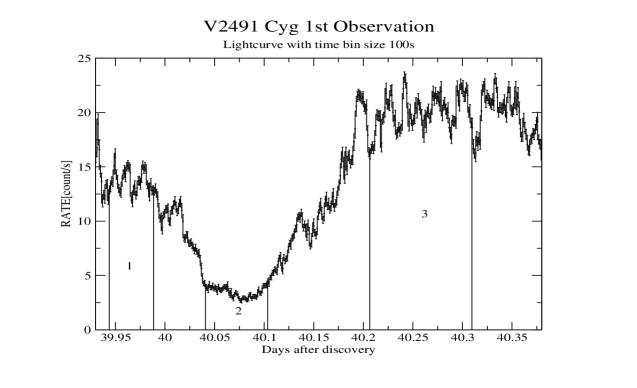
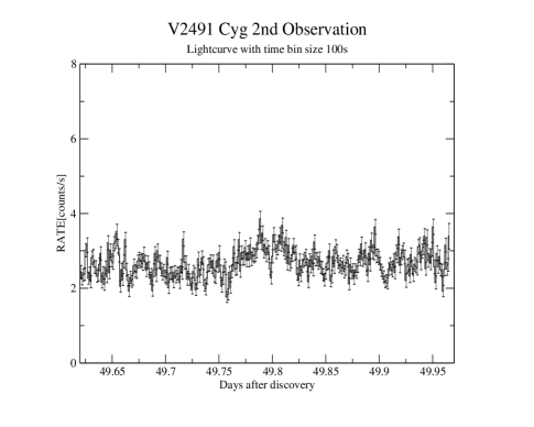
Figure 1: The XMM-Newton RGS1 light curve (LC) of V2491 Cyg. First observation (40 d after outburst) is on the left and the second observation is on the right (50 d after outburst). The three different regions of count rates are labeled as 1, 2, and 3 on the LC of the first observation as assumed in the spectral analysis.

3 Analysis and Results

3.1 Photoionized and collisionally ionized absorber models

SPEX is a software package (version 2.05.04; Kaastra et al. 1996) optimized for the analysis and interpretation of high-resolution cosmic X-ray spectra. The software is especially suited for fitting spectra obtained by current X-ray observatories like XMM-Newton, $Chandra$, and $Suzaku$. It is maintained by SRON (HEA Division, Netherlands Institute for Space Research).

We obtained a similar model description to Pinto et al. (2012) to fit both sets of the nova data (first and second observation) in order to compare the different ionized absorber components in the system. There are two main models in SPEX that can be used to model ionized intrinsic absorption; one of them is the xabs (used by Pinto et al. 2012) and the other is the Hot model used in this study. The xabs model of SPEX calculates the warm, photoionized absorption by a thin slab composed of different ions located between the ionizing source and the observer. The xabs model assumes a small angle subtended by the slab at the source so that only absorption and scattering out of the line-of-sight by the slab are considered. The processes taken into account are the continuum and the line absorption by the ions and scattering out of the line-of-sight by the free electrons in the slab. The transmission, T, of the slab is calculated as $T=\exp[-\tau_{\rm c}-\tau_{\rm l}-\tau_{\rm e}]$, here $\tau_{\rm c}$ and $\tau_{\rm l}$ are the total continuum and line optical depth, respectively, and $\tau_{\rm e}$ is the electron scattering optical depth. For $\tau_{\rm e}$ the classical Thomson approximation is valid below 10 keV (longer than 1.24 Å ). Most continuum opacities are taken from Verner & Yakovlev (1995), while line opacities and wavelengths for most ions are taken from Verner et al. (1996) and abundances are calculated using Lodders $\&$ Palme (2009) (see the details and additional references in the SPEX user’s manual). $\tau_{\rm l}$ is a function of v and $\sigma_{\rm v}$ which are free parameters of xabs. v is the average systematic velocity shift of the absorber, in km s^-1. Negative and positive values of v correspond to blue and red shifts, respectively. $\sigma_{\rm v}$ is the turbulent velocity broadening of the absorber in km s^-1, defined as $\sigma_{\rm total}^{2}=\sigma_{\rm v}^{2}+\sigma_{\rm thermal}^{2}$, where $\sigma_{\rm total}$ is the total width of a line and $\sigma_{\rm thermal}$ the thermal contribution. The relative column densities of the ions are calculated through a photoionization model introducing two free parameters: N${}_{\rm H^{xabs}}$ and $\xi$. N${}_{\rm H^{xabs}}$ is the equivalent hydrogen column density of the ionized absorber in units of atoms cm^-2. $\xi$ is the ionization parameter of the absorber defined as $\xi=L/n_{\rm e}\leavevmode\nobreak\ r^{2}$, where L is the luminosity of the ionizing source, n_e the density of the plasma and r the distance between the slab and the ionizing source. $\xi$ is expressed in units of erg cm s^-1. Codes such as XSTAR (Kallman & Bautista 2001) or CLOUDY (Ferland 2003) are used for the broad-band ionizing continuum from infrared to hard X-rays where the ionic column densities of a photoionized slab is precalculated for different values of $\xi$ and used in the fitting procedure with SPEX. During the fitting process, SPEX reads in the grid of precalculated ionic column densities and finds the best set and the best-fit values for $N{\rm{}_{H}^{xabs}}$ and $\xi$.

In order to compare with the analysis using xabs models, here, we focus mainly on the Hot model within SPEX that assumes a collisional ionization (equilibrium) absorber model instead of the photoionized absorber model. This model calculates the transmission of a plasma in collisional equilibrium with cosmic abundances. For a given temperature and abundances, the model calculates the ionization balance and then determines all ionic column densities by scaling the prescribed hydrogen column density. Using these column densities, the transmission of the plasma is calculated by multiplying the transmission of the individual ions. The transmission assumes both continuum and line opacity. Most continuum opacities are taken from Verner & Yakovlev (1995), while line opacities and wavelengths for most ions are taken from Verner et al. (1996) and abundances are calculated using Lodders $\&$ Palme (2009). This model will mimic neutral plasma transmission at about 0.0005 keV (6000 K) which we utilize to model the gas component of the interstellar absorption. It, also, has similar free parameters to xabs model like velocity shift v and turbulent velocity broadening $\sigma_{\rm v}$ together with equivalent hydrogen column density N${}_{\rm H^{Hot}}$ and kT, temperature of the absorber in keV.

3.2 XMM-Newton RGS Spectrum of V2491 Cyg

As outlined in section [2.0], we analyzed the data using Science Analysis Software (SAS) version 14.0.0 and produced RGS1-2 spectra and relevant response matrices using rgsproc and rgsfluxer for different spectral orders. Some spectral analysis checks were performed using XSPEC (Arnaud 1996) version 12.9.0, and the main analyses were conducted with the SPEX software package (Kaastra et al. 1996) version 2.05.04 . In order to perform the analysis with SPEX, RGS1 and RGS2 first order spectra were combined by using tasks rgsfluxcombine and rgsfmat within SPEX. The fluxed spectra were created between 5-38 Å with 3400 bins. In general, the spectra between 7-38 Å (0.3-1.8 keV) were used for the fitting process and the data were binned by a factor of 4 between 7-11 Å  and by a factor 2 for 11-38 Å . The detailed description of the emission and absorption lines and edges, can be found in Ness et al. (2011) and Pinto et al. (2012).

Our main aim is to study the complex absorption properties in the high resolution X-ray spectra of classical and recurrent novae and our target, in this work, is V2491 Cyg. In order to compare with the absorption modeling used in Pinto et al. (2012) which used the photoionized absorber model xabs, we used the absorption model Hot which is a collisionally ionized (in equilibrium) absorber model in the SPEX software package. Since a comparative study with the xabs models would require that the data are analyzed and fitted in the same manner, we followed the analysis steps and used the same modeling in Pinto et al. (2012) except for the photoionized absorber models. We utilized a composite model that includes a blackbody model Bb for the continuum and a plasma emission model in collisional equilibrium Cie for the excess in the harder X-ray band together with two Hot absorber models, one Amol model for the dust absorption (Pinto et al. 2010) in the line of sight and finally another Hot model with a very low temperature ($\sim$ 1eV) that would mimic the cold gas absorption in the interstellar medium. We followed a similar fitting procedure to Pinto et al. (2012). First the harder X-ray band data (7-14.4 Å) was fitted with the Cie model together with the cold Hot (Hot-ISM) absorber model for the gas in the interstellar medium to determine the abundances separately from the other absorber models using the fluxed spectrum of region3 and the second observation. An additional blackbody model Bb was added in the fitting process for the second observation to account for the long wavelength excess. If the additional blackbody model was not included, the $\chi_{\nu}^{2}$ of the fit was 2.15 and not acceptable. Figure 2 shows the fitted models to the two data sets. We find that the spectral parameters of this blackbody emission are different than the main blackbody model parameters of the stellar remnant presented in Table 1 (& 2). The norm is (2.0-4.0)$\times$10¹⁵ cm², temperature is (120-131) eV and the luminosity is 6.0$\times$10³⁵ erg s^-1. However, inclusion of this component in the fitting procedure in the total RGS band 7-38 Å does not affect the spectral parameters in Table 1 (& 2), particularly the main stellar remnant emission, and it only improves the fits at about 93$\%$ confidence level. The spectral parameters of this new blackbody component remain similar in the 90$\%$-95$\%$ confidence level when fitted in the 7-14 Å or 7-38 Å energy range. We elaborate on this component in the discussion section.

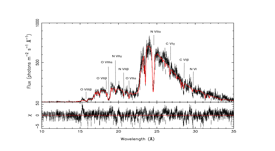
Figure 3: The RGS1+2 fluxed spectrum of V2491 Cyg using region1 of the LC (first observation) fitted with the composite model described in the text using the Hot model in SPEX (see Table 1). Certain detected blueshifted absorption lines are labeled with dashed lines.

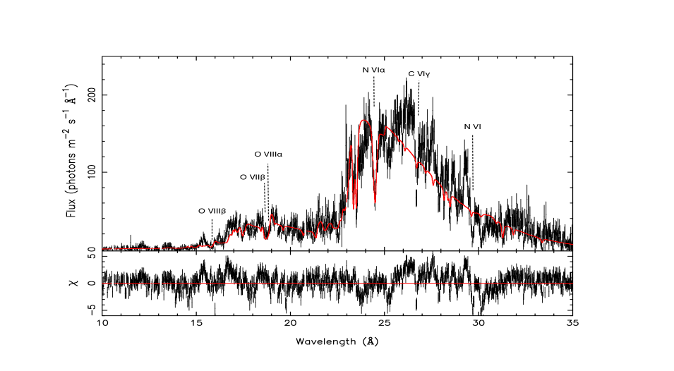
Figure 4: The RGS1+2 fluxed spectrum of V2491 Cyg using region2 of the LC (first observation) fitted with the composite model described in the text using the Hot model in SPEX (see Table 1). Certain detected blueshifted absorption lines are labeled with dashed lines.

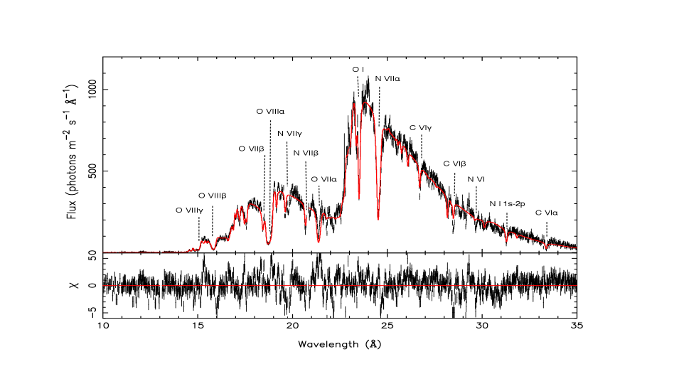
Figure 5: The RGS1+2 fluxed spectrum of V2491 Cyg using region3 of the LC (first observation) fitted with the composite model described in the text using the Hot model in SPEX (see Table 1). Certain detected blueshifted absorption lines are labeled with dashed lines.

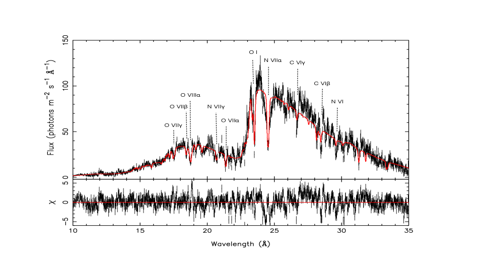
Figure 6: The RGS1+2 fluxed spectrum of V2491 Cyg obtained from the second observation fitted with the composite model described in the text using the Hot model in SPEX (see Table 1). Certain detected blueshifted absorption lines are labeled with dashed lines.

The Ne and Mg abundances from these fits above (i.e., using region3 and second observation spectra) were fixed together with the $v_{\rm mic}$ parameter for the fits using fluxed spectra of regions 1 and 2. Note that the free fits yield very similar abundances of Ne and Mg for the second observation. Following this, first the fluxed spectrum of region3 was fitted with the composite model Hot-ISM$\times$(Cie+(Hot-1$\times$Hot-2)$\times$(Bb)) and once the fit converged the multiplicative model Amol was added and a final fit was performed Amol$\times$Hot-ISM$\times$(Cie+(Hot-1$\times$Hot-2)$\times$(Bb)). Next, the elemental abundances derived for the Hot absorber models using the fit to the fluxed spectrum of region3 were fixed for all the fits to the fluxed spectra of the regions 1, 2 and the second observation assuming that the abundances in the ejecta/wind will stay the same in the short duration of the X-ray observation, and that the second observation is only 10 days after the first observation. The fitted fluxed spectra of V2491 Cyg can be found in Figures 3-6 where Figure 3-5 are for regions 1, 2, and 3 as labeled in Figure 1 (left panel) for the first observation. Figure 6 is the spectral fit to the fluxed spectrum of the second observation. The resulting spectral parameters from fits with the composite model using the collisionally ionized (in equilibrium) hot absorber models are listed in Table 1. All abundances are given in Solar units. The error ranges of the spectral parameters are given at the 90$\%$ confidence level for a single parameter ($\Delta\chi^{2}$=2.71). The degrees of freedom are taken in accordance with the Pinto et al. (2012) fits for comparison. However, we assumed abundances in Solar units which takes H as the reference element instead of using oxygen as the reference.

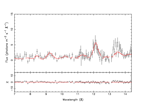
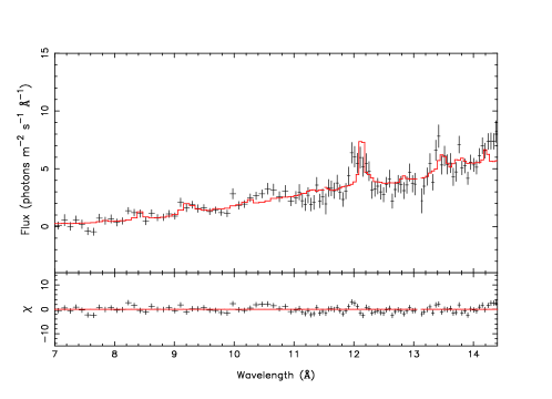
Figure 2: The RGS1+2 fluxed spectrum of V2491 Cyg fitted in the range 7-14.4 Å using the plasma emission model Cie and the cold Hot-ISM absorption model. A blackbody model of emission was also used as an additive model for the second observation spectrum. The left hand and right hand panels show the fit to the fluxed spectrum of region3 and second observation data, respectively.

We find that our fits yield $\chi_{\nu}^{2}$=1.8-2.9 (for about 1440 degrees of freedom) using the collisionally ionized hot intrinsic absorber models for the classical nova V2491 Cyg. Given the $\chi_{\nu}^{2}$ values, the collisionally ionized absorber models yield considerably better fits to these data sets of V2491 Cyg than the photoionized absorber fits in Pinto et al. (2012) which have $\chi_{\nu}^{2}$ in a range 2.3-7.0 for about 1470 degrees of freedom. Other modeling using expanding atmosphere models (van Rossum & Ness 2010) yielded very high values of $\chi_{\nu}^{2}$ not given in the paper and the NLTE static atmosphere fits in Ness et al. (2011) had a $\chi_{\nu}^{2}$ range of 2.2-21.8 for about 5600 degrees of freedom. We note that the comparison with the Pinto et al. (2012) results using the photoionized absorbers indicates that particularly, for the fits to the region1 and region3 spectra where the count rates are the highest, inclusion of the collisionally ionized hot absorbers improves the fits to a good extent, the improvements for the low count rate region2 and the second observation data with the lowest count rate are rather less obvious. We believe this is because the high count rate data show the absorption and emission features (along with a strong continuum) more prominently allowing for better fitting of the detailed models using the high spectral resolution data. Such high spectral resolution data with low count rates have increased statistical errors with the detailed spectral features more smeared out or less visible (with weaker continuum) which does not allow for the fit quality to differentiate between several models appropriately. However, in all four spectra that we have fitted, we have better $\chi_{\nu}^{2}$ values in comparison with the intrinsic photoionized absorber fits in Pinto et al. (2012). An FTEST (within XSPEC) can be performed to test the significance of improvement of these fits with respect to the photoionized absorber fits in Pinto et al. (2012). Comparison of the $\chi^{2}$ and degrees of freedom of each fit for regions 1-3, the FTEST probability ranges between 3$\times$10^-26-6$\times$10^-270 which is the value of 1-(confidence level). Thus, the improvement is much better than 10$\sigma$ where 3$\sigma$ significance would have FTEST probability of $\sim$ 0.003 . However, the FTEST for the fits to the lowest count rate data (the second observation) gives a probability of 0.4 (about 60% confidence level) which yield only around 1$\sigma$ improvement for the collisionally ionized absorber fits over the photoionized absorber fits.

In addition, we tested the possibility of having a third absorber by adding another Hot model to the fits in Table 1 and tested the significance of this component by applying an FTEST. We find that the fits to the data of region 1, 2, and the second observation yield improvement of $\chi^{2}$ values at a confidence level less than 30%. However, FTEST for the fit of the region3 spectrum resulted in a probability of 5$\times$10^-8 yielding an improvement over 5$\sigma$.

Our original idea, as described in the Introduction section, was a composite model where there is complex absorption of interstellar, photospheric, and of collisionally-ionized and/or photoionized gas originating from the moving material in the line of sight from a nova wind or ejecta. As a result, our goal was to model the absorption components detected in the high resolution spectra independently from the continuum model (i.e., mainly stellar remnant emission) and compare the photoionized warm and collisionally ionized hot absorber gas. Thus, next, we employed the xabs model for the third absorber in V2491 Cygni ( Amol$\times$Hot-ISM$\times$(Cie+(Hot-1$\times$Hot-2$\times$xabs)$\times$(Bb))). This composite model implies that there is some absorption from photoionized gas along with the main absorbers that are collisionally ionized. For this additional model, we used a grid of ionic column densities for xabs calculated utilizing the CLOUDY software assuming an ionizing continuum of blackbody radiation at 65 eV $(7.8\times 10^{5}K)$ chosen inaccordance with our analysis. The resulting fits show that all the $\chi_{\nu}^{2}$ values except the region2 fit (FTEST probability is 0.005 yielding an improvement at 99.5$\%$ confidence level) are improved over 10$\sigma$ significance (using FTESTs the probability is 3.2$\times$10^-12-6.9$\times$10^-47). These improved fits are given in Table 2. We note here that the spectral parameters (in Table 1 & 2) of the main stellar remnant emission (Bb), plasma emission Cie, the interstellar dust Amol and Hot-ISM gas absorption remain consistent within 90$\%$-95$\%$ confidence level errors.

Finally, we note that Pinto et al. (2012) have attempted to use stellar atmosphere models instead of blackbody models using particular CNO abundances along with the complex absorption model they have used. They report that such models only resulted in higher $\chi_{\nu}^{2}$ values and have not improved the fits at all.

Table 1: The spectral parameters obtained from the composite model fits including two Hot absorber models to the RGS spectrum of V2491 Cyg (errors are calculated at the 90% confidence level.)

Model	Parameters	Region1	Region2	Region3	$2^{nd}$ Obs.
Blackbody	Norm ($10^{20}\rm cm^{2}$)	$1.53^{+0.39}_{-0.25}$	$0.23^{+0.86}_{-0.04}$	$0.40^{+0.47}_{-0.21}$	$0.02^{+0.05}_{-0.01}$
	Temperature (eV)	$68.5^{+0.9}_{-0.9}$	$64.5^{+0.6}_{-3.6}$	$88.4^{+2.7}_{-1.8}$	$75.7^{+9.1}_{-6.5}$
	Luminosity($10^{39}$ erg s-1)	2.18	0.23	1.92	0.05
CIE	Norm ($10^{58}\rm cm^{-3}$)	$0.40^{+0.11}_{-0.09}$	$0.72^{+0.79}_{-0.32}$	$0.42^{+0.13}_{-0.05}$	$0.27^{+0.06}_{-0.1}$
	Temperature (keV)	$0.20^{+0.01}_{-0.01}$	$0.16^{+0.03}_{-0.02}$	$0.20^{+0.01}_{-0.01}$	$0.30^{+0.13}_{-0.03}$
	$v_{mic}$ (km s-1)	2791	2791	$2791^{+333}_{-288}$	$25068^{+1383}_{-951}$
	Ne Abundance	2.45	2.45	$2.45^{+1.36}_{-0.92}$	$2.4^{+0.9}_{-0.9}$
	Mg Abundance	1.2	1.2	$1.2^{+1.0}_{-0.6}$	$1.98^{+0.70}_{-0.70}$
	Luminosity($10^{36}$ erg s-1)	1.31	1.78	1.38	0.77
HOT-1	$N_{H}$ ($10^{24}\rm cm^{-2}$)	$0.40^{+0.03}_{-0.03}$	$0.09^{+0.03}_{-0.01}$	$0.07^{+0.01}_{-0.01}$	$0.19^{+0.10}_{-0.02}$
	Temperature (keV)	$2.63^{+0.96}_{-0.56}$	$1.77^{+0.17}_{-0.12}$	$1.06^{+0.03}_{-0.03}$	$1.38^{+0.58}_{-0.12}$
	$\sigma_{v}$ rms velocity (km s-1)	$872^{+25}_{-24}$	$827^{+61}_{-86}$	$879^{+12}_{-12}$	$114^{+18}_{-15}$
	velocity shift (km s-1)	$-3186^{+51}_{-50}$	$-3699^{+113}_{-173}$	$-3128^{+30}_{-31}$	$-2636^{+47}_{-45}$
HOT-2	$N_{H}$ ($10^{24}\rm cm^{-2}$)	$0.86^{+0.03}_{-0.03}$	$0.18^{+0.01}_{-0.02}$	$1.80^{+0.02}_{-0.02}$	$0.51^{+0.02}_{-0.05}$
	Temperature (keV)	$0.81^{+0.03}_{-0.03}$	$0.58^{+0.07}_{-0.11}$	$0.99^{+0.03}_{-0.03}$	$0.82^{+0.05}_{-0.45}$
	$\sigma_{v}$ rms velocity (km s-1)	$54^{+8}_{-9}$	$<9$	$56^{+4}_{-5}$	$60^{+7}_{-8}$
	velocity shift (km s-1)	$-3180^{+71}_{-58}$	$-3038^{+6}_{-183}$	$-3194^{+30}_{-31}$	$-3550^{+36}_{-33}$
Abundances	C Abundance	0.43	0.43	$0.43^{+0.07}_{-0.07}$	0.43
	N Abundance	5.2	5.9	$5.9^{+0.5}_{-0.9}$	5.9
	O Abundance	37.9	37.9	$37.9^{+5.8}_{-10.0}$	37.9
	Si Abundance	0.02	0.02	$<0.02$	0.02
	S Abundance	0.02	0.02	$0.02^{+0.01}_{-0.01}$	0.02
	Ar Abundance	1.6	1.6	$1.6^{+3.9}_{-1.2}$	1.6
	Ca Abundance	0.01	0.01	$<0.01$	0.01
	Fe Abundance	8.9	8.9	$8.9^{+3.8}_{-2.1}$	8.9
HOT-ISM	$N_{H}$ ($10^{21}\rm cm^{-2}$)	$3.89^{+0.06}_{-0.06}$	$3.84^{+0.06}_{-0.19}$	$3.26^{+0.05}_{-0.09}$	$2.4^{+0.3}_{-0.2}$
	Temperature (eV)	$1.11^{+0.03}_{-0.04}$	$1.20^{+0.02}_{-0.04}$	$1.01^{+0.02}_{-0.02}$	$0.8^{+0.3}_{-0.3}$
	N Abundance	1.16	1.16	$1.16^{+0.12}_{-0.12}$	1.16
	O Abundance	1.75	1.75	$1.75^{+0.04}_{-0.02}$	1.75
	Fe Abundance	0.95	0.95	$0.95^{+0.13}_{-0.12}$	0.95
AMOL (Dust)	$O_{2}$ ($10^{17}\rm cm^{-2}$)	$0.34^{+0.13}_{-0.13}$	$2.3^{+0.2}_{-0.2}$	$<0.1$	$1.3^{+0.1}_{-0.1}$
	$H_{2}O(ice)$ ($10^{17}\rm cm^{-2}$)	$5.5^{+0.3}_{-0.3}$	$7.8^{+0.5}_{-0.5}$	4.77${}^{+0.13}_{-0.13}$	$7.2^{+0.2}_{-0.2}$
	$CO$ ($10^{17}\rm cm^{-2}$)	$1.28^{+0.13}_{-0.13}$	$0.27^{+0.2}_{-0.2}$	$0.1^{+0.07}_{-0.06}$	$<0.1$
	$\chi_{\nu}^{2}$	1.80	2.4	2.86	2.3
	(d.o.f.)	(1415)	(1439)	(1440)	(1465)

Table 2: The spectral parameters obtained from the composite model fits including two Hot absorber and one xabs models to the RGS spectra of V2491 Cyg (errors are calculated at the 90% confidence level.)

Model	Parameters	Region1	Region2	Region3	$2^{nd}$ Obs.
Blackbody	Norm ($10^{20}\rm cm^{2}$)	$0.99^{+0.06}_{-0.06}$	$0.46^{+0.05}_{-0.05}$	$0.40^{+0.01}_{-0.01}$	$0.02^{+0.01}_{-0.01}$
	Temperature (eV)	$68.1^{+0.5}_{-0.5}$	$63.1^{+1}_{-0.8}$	$84.6^{+0.4}_{-0.4}$	$79.9^{+1.2}_{-1.2}$
	Luminosity($10^{39}$ erg/s)	1.37	0.43	1.57	0.06
CIE	Norm ($10^{58}\rm cm^{-3}$)	$0.97^{+0.47}_{-0.37}$	$1.14^{+0.71}_{-0.40}$	$0.42^{+0.13}_{-0.05}$	$0.55^{+0.04}_{-0.04}$
	Temperature (keV)	$0.18^{+0.02}_{-0.01}$	$0.17^{+0.02}_{-0.02}$	$0.19^{+0.01}_{-0.01}$	$0.26^{+0.01}_{-0.01}$
	$v_{\rm mic}$ (km s-1)	2914	2914	$2914^{+612}_{-510}$	$22410^{+1688}_{-1466}$
	Ne Abundance	2.45	2.45	$2.45^{+1.36}_{-0.92}$	$2.4^{+0.9}_{-0.9}$
	Mg Abundance	1.2	1.2	$1.2^{+1.0}_{-0.6}$	$1.98^{+0.70}_{-0.70}$
	Luminosity($10^{36}$ erg s-1)	1.34	1.49	1.18	0.88
HOT-1	$N_{H}$ ($10^{24}\rm cm^{-2}$)	$0.08^{+0.01}_{-0.01}$	$0.13^{+0.26}_{-0.05}$	$0.06^{+0.01}_{-0.01}$	$0.16^{+0.69}_{-0.02}$
	Temperature (keV)	$0.95^{+0.04}_{-0.04}$	$2.48^{+0.52}_{-0.35}$	$0.94^{+0.02}_{-0.02}$	$1.19^{+0.86}_{-0.20}$
	$\sigma_{v}$ rms velocity (km s-1)	$892^{+43}_{-41}$	$634^{+131}_{-156}$	$932^{+23}_{-23}$	$133^{+31}_{-28}$
	velocity shift (km s-1)	$-3304^{+83}_{-83}$	$-3805^{+229}_{-278}$	$-3250^{+51}_{-51}$	$-2826^{+88}_{-97}$
HOT-2	$N_{H}$ ($10^{24}\rm cm^{-2}$)	$0.76^{+0.02}_{-0.02}$	$0.44^{+0.05}_{-0.24}$	$1.61^{+0.01}_{-0.01}$	$0.71^{+0.01}_{-0.14}$
	Temperature (keV)	$0.89^{+0.05}_{-0.04}$	$0.59^{+0.02}_{-0.1}$	$1.06^{+0.02}_{-0.02}$	$0.68^{+0.01}_{-0.19}$
	$\sigma_{v}$ rms velocity (km s-1)	$<37$	$<20$	$35^{+14}_{-18}$	$<17$
	velocity shift (km s-1)	$-3309^{+84}_{-103}$	$-3073^{+161}_{-191}$	$-3334^{+38}_{-36}$	$-3660^{+75}_{-65}$
XABS	$N_{H}$ ($10^{20}\rm cm^{-2}$)	$2.68^{+0.4}_{-0.3}$	$3.85^{+40}_{-2.56}$	$2.79^{+0.1}_{-0.1}$	$0.56^{+0.06}_{-0.06}$
	Log $\xi$ (erg cm s-1)	$2.04^{+0.14}_{-0.16}$	$3.64^{+1.35}_{-0.2}$	$2.18^{+0.05}_{-0.05}$	$0.41^{+0.08}_{-0.07}$
	$\sigma_{v}$ rms velocity (km s-1)	$49^{+126}_{-18}$	$<15831$	$53^{+10}_{-9}$	$195^{+78}_{-58}$
	velocity shift (km s-1)	$-3013^{+100}_{-368}$	$-1093^{+1294}_{-343}$	$-2968^{+47}_{-44}$	$-3127^{+127}_{-118}$
Abundances	C Abundance	0.38	0.38	$0.38^{+0.07}_{-0.07}$	0.38
	N Abundance	5.8	5.8	$5.8^{+0.2}_{-0.2}$	5.8
	O Abundance	15.9	15.9	$15.9^{+0.5}_{-0.5}$	15.9
	Si Abundance	0.06	0.06	$<0.06$	0.06
	S Abundance	0.02	0.02	$0.02^{+0.02}_{-0.01}$	0.02
	Ar Abundance	0.5	0.5	$<0.5$	0.5
	Ca Abundance	0.02	0.02	$<0.02$	0.02
	Fe Abundance	8.9	8.9	$8.9^{+3.8}_{-2.1}$	8.9
HOT-ISM	$N_{H}$ ($10^{21}\rm cm^{-2}$)	$3.81^{+0.05}_{-0.05}$	$4.15^{+0.05}_{-0.06}$	$3.31^{+0.02}_{-0.02}$	$2.4^{+0.1}_{-0.1}$
	Temperature (eV)	$1.09^{+0.07}_{-0.3}$	$1.20^{+0.03}_{-0.05}$	$1.01^{+0.04}_{-0.04}$	$0.8^{+0.1}_{-0.1}$
	N Abundance	1.12	1.12	$1.12^{+0.13}_{-0.14}$	1.12
	O Abundance	1.68	1.68	$1.68^{+0.02}_{-0.02}$	1.68
	Fe Abundance	0.81	0.81	$0.81^{+0.13}_{-0.12}$	0.81
AMOL (Dust)	$O_{2}$ ($10^{17}\rm cm^{-2}$)	$0.47^{+0.61}_{-0.03}$	$1.48^{+0.23}_{-0.24}$	$<0.4$	$0.9^{+0.1}_{-0.1}$
	$H_{2}O(ice)$ ($10^{17}\rm cm^{-2}$)	$5.1^{+1.2}_{-0.1}$	$7.4^{+0.5}_{-0.5}$	4.65${}^{+0.3}_{-0.7}$	$6.4^{+0.2}_{-0.2}$
	$CO$ ($10^{17}\rm cm^{-2}$)	$1.34^{+0.53}_{-0.03}$	$0.29^{+0.2}_{-0.2}$	$0.16^{+0.07}_{-0.06}$	$<0.2$
	$\chi_{\nu}^{2}$	1.73	2.38	2.46	2.06
	(d.o.f.)	(1411)	(1435)	(1436)	(1463)

4 Discussion

In a nova explosion, convection and radiation pressure leads to the ejection of the envelope material, forming an optically thick/thin shell which the high energy photons produced by the nuclear burning have to travel through. The resultant spectrum is an atmospheric spectrum originating from the photosphere with a blackbody-like continuum and superimposed absorption lines as detected by the X-ray grating data (aside from the hard X-ray component originating from the ejecta/winds). In the X-ray spectral analysis of novae data, first attempts to derive spectral parameters were done using blackbody models indicating/yielding super-Eddington luminosities for the stellar remnant (see, Oegelman et al. 1993). In order to overcome the super-Eddington luminosity problem and to incorporate the abundance and ionization edge effects of C-O and O-Ne core WDs, LTE (Local Thermodynamic Equilibrium) models were used with the ROSAT and Beppo-Sax data and successful results were attained (e.g., Balman et al. 1998; Kahabka et al. 1999; Balman & Krautter 2001). However, these data had crude spectral resolution, and only after obtaining stellar remnant spectra with the X-ray gratings, the very detailed structure with emission and absorption features were recovered. After this, the few attempts to derive spectral parameters from the stellar remnants have been done using hydrostatic NLTE atmosphere models (Orio et al. 2002; Nelson et al. 2008; Rauch et al. 2010; Osborne et al. 2011; Ness et al. 2011; Tofflemire et al. 2013) that would account for the absorption edges/lines from a static atmosphere. However, the detailed structure in the spectra was very difficult to model and results yielded best approximations to the observed spectra with large $\chi_{\nu}^{2}$ values in the fitting process. In addition, most absorption features showed blueshifts in the spectra (e.g., Ness et al. 2003, 2007) not modeled by the NLTE static atmosphere models where only the static photospheric absorption lines were taken into account (for the analysis of the spectra using static atmospheres, the spectra themselves had to be shifted for a fixed blueshift).

In order to compensate for the inadequacies, the stellar atmosphere code PHOENIX (Hauschildt & Baron 1999, 2004) was adjusted to model NLTE expanding atmosphere models, a hybrid atmosphere model that is hydrostatic at the base with an expanding envelope on the top. Expansion is attained by an optically thick wind from the remnant. These models have been used to fit the detailed spectral data with yet again best approximations yielding estimated spectral parameters (e.g., Petz et al. 2005; van Rossum & Ness 2010). van Rossum (2012) presents a new set of expanding NLTE atmosphere models with better quality fit approximations but yet with solar composition models. One important outcome of this modeling was that dynamic models resulted in lower effective temperatures for the remnant WD in comparison with the static models. This is largely due to existing edges and lines being too strong in the static case than the expanding envelope case where features were weak. This can cause the static models to measure higher temperatures than normal in order to account for the harder X-ray tails in the observed spectra (van Rossum & Ness 2010; van Rossum 2012).

Our approach is to mainly model the absorption components in the X-ray spectroscopic data. This is an independent approach regarding the choice of the continuum emission with the atmosphere models being expanding or static. We are assuming a simple continuum model, a blackbody emission model together with a plasma emission model (collisional equilibrium), so that the complicated absorption models are thoroughly investigated. We note that a blackbody model does not include absorption features that could exist in the stellar atmosphere emission, thus we will be missing some of the atmospheric absorption features. We note that SPEX software does not have user defined models and thus, we have no means of publicly adding atmosphere models to use within the software. We model the blueshifted absorption features in the line of sight as in a nova wind or expanding ejecta. We infer, for this case of V2491 Cyg, two main collisionally ionized hot absorbers and an additional photoionized component along with absorption from interstellar neutral hydrogen column density of cold gas and dust (separately) in the line of sight. We compare and contrast our results with the spectral parameters from different modeling that exists in the literature, particularly with Pinto et al. (2012) that has analyzed the same data using only photoionized absorbers.

In comparison with the modeling using three photoionized absorption components used by Pinto et al. (2012), our fits yield better $\chi_{\nu}^{2}$ (with similar degrees of freedom) for all the regions 1, 2, 3 and the second observation (see Tables 1 & 2). Our findings on the plasma continuum emission parameters using the Cie model, and the absorption properties using the Hot-ISM, and Amol dust absorption models are similar to the results of Pinto et al. (2012). We take that the difference in the quality of the fits has to do with the assumption of the utilized intrinsic absorption models. Thus, we suggest that the major absorber in V2491 Cyg are associated with the shocked and collisionally ionized nova ejecta and the wind which would also be consistent with the large velocity blueshifts and turbulent line broadening, we obtained from our fits. An additional photoionized warm absorber model improves the fits indicating that there is also some contribution to the complex absorption from photoionized gas in the expanding shell/ejecta.

The best fit model for V2491 Cyg using optically thick wind models to fit the X-ray, near infrared, and optical light curves assumes 1.3$\pm$0.02 M_⊙ for a chemical composition of X=0.20, Y=0.48, X_CNO=0.2, X_Ne=0.1, Z=0.02 (Hachisu & Kato 2010). The fits with the blackbody emission model to the Swift data yield photospheric temperatures on day 39 of 36-40 eV (4.3-4.8$\times 10^{5}$ K), day 53 of 73-83 eV (8.8-10.0$\times 10^{5}$ K) and day 80-109 of 76-81 eV (9.1-10.0$\times 10^{5}$ K) (Page et al. 2010). The XMM-Newton data used in our work are obtained on day 40 and 50 for which we derive a blackbody temperature of 61-91 eV (7.3-10.1$\times 10^{5}$ K) and 69-85 eV (8.3-10.0$\times 10^{5}$ K), respectively. These ranges have remained the same, but narrowed down slightly to 62-85 eV for day 40 and 78-82 to day 50 when an additional xabs model was introduced. The value (blackbody temperature) for day 40 is larger than the value obtained from Swift on day 40, but is in accordance with the Swift value obtained for day 53. Our effective temperature values are larger compared with the effective temperature of 6$\times 10^{5}$ K obtained from the best fit approximations to the XMM-Newton  data (day 50) using expanding NLTE atmosphere models (van Rossum & Ness 2010). In comparison with the fits using NLTE static atmosphere models where effective temperatures of (9.6-10.5)$\times 10^{5}$ K are achieved (Ness et al. 2011), our temperatures are lower including the best fit values. The temperature ranges obtained using the fits with photoionized absorbers are 81-123 eV for day 40 and 94-96 eV (9.6-10.5$\times 10^{5}$ K) for day 50 (Pinto et al. 2012) which are high, in general. Our fitted results with the two Hot models for a collisionally ionized (in equilibrium) absorber yield abundances of C/C_⊙=0.3-0.5, O/O_⊙=28-43, and N/N_⊙=5-7. When we introduce the third photoionized absorber component, the abundance of the carbon and nitrogen remain the same, but the oxygen abundance becomes O/O_⊙=15-17. These values are determined from material in absorption. We find that carbon is subsolar and N supra-solar consistent with the effects of H-burning (i.e., depletion of C and enhancement of N). The high oxygen content hints at the existence of an underlying C-O WD. Munari et al. (2011) calculated elemental abundances of V2491 Cyg using ground-based optical observations. They found Fe/Fe_⊙=0.6, O/O_⊙=4.3, N/N_⊙=59, and Ne/Ne_⊙=6.5. van Rossum & Ness (2010)  have only assumed solar abundances for simplicity while working with the NLTE expanding atmosphere models and Ness et al. (2011) have found consistent fits using static NLTE atmosphere models with fixed abundances where oxygen abundance was in a range O/O_⊙=10-30. This latter model has similar abundances to what we derived in this study.

Aside from the effective temperatures of the blackbody emission, we can derive the effective radius of the blackbody emitting region to infer the WD radius. The normalization of the blackbody model fits in Table 1 & 2 is equal to 4$\pi$R². As a result, the effective radius limits are in a range (32-39)$\times 10^{8}$ cm for the region1 data, (12-29)$\times 10^{8}$ cm for the regions 2, 3 on day 40 and (2.8-7.5)$\times 10^{8}$ cm on day 50 (within the 90% confidence error ranges). The addition of a third absorber component xabs, slightly modifies these ranges to (27-30)$\times 10^{8}$ cm for the region1 data, (17-20)$\times 10^{8}$ cm for the regions 2, 3 on day 40 and (2.8-4.9)$\times 10^{8}$ cm on day 50. The progressive change (getting smaller in time) of radius by a factor of about 5-10 (within errors) in about 10 days is notable. Such a fast decrease in effective stellar remnant radius by about a factor of 2-3 within a week was detected for the moderately fast nova V1974 Cyg (N Cyg 1992) (Balman et al. 1998). Balman et al. (1998) also notes radii in excess of 1$\times 10^{9}$ cm hinting at a bloated WD during the early H-burning phases of the outburst. The effective blackbody temperatures that are in a range 61-91 eV (taking the largest range from Tables 1 & 2) on day 40 and 50 constrain the WD mass in a range 1.15-1.3 M_⊙ consistent with the fast nature of the nova. For this calculation we assumed that the temperature range is the maximum temperature achieved by the H-burning WD and utilized the equation (3) in Balman et al. (1998) that relates maximum effective temperature with WD mass. We underline that the radius range for the stellar remnant, on day 50, shows the desired range for the radius of a C-O WD which is (4.5-2.8)$\times 10^{8}$ cm for the mass range of 1.15-1.3 M_⊙ (Hamada & Salpeter 1961; Panei et al. 2000). Our model fits predict super-Eddington luminosities (see Table 1 & 2) as found in all blackbody model fits, in general. The SPEX assumes a given distance to the source fixed in the fitting procedure, 10.5 kpc (Darnley et al. 2011); a smaller distance will decrease these luminosity values further. A recent distance estimate toward this source is 2.1-3.5 kpc (Özdönmez et al. 2016) which yields a decrease by a factor of 10-25 in the luminosities, reducing our values to the Eddington limit.

We find an interstellar neutral hydrogen column density (in the line of sight, using the Hot-ISM model) for V2491 Cyg of about (3.2-4.2)$\times 10^{21}$ cm^-2 for day 40 and (2.2-2.7)$\times 10^{21}$ cm^-2 for day 50 from our fits (see Tables 1 & 2). We used the colden (http://cxc.harvard.edu/toolkit/colden.jsp) and nhtot (http://www.swift.ac.uk/analysis/nhtot/) interactive program to calculate the column density of hydrogen in the direction of V2491 Cyg. The colden program utilizes Stark et al. (1992) and Dickey & Lockman (1990) and nhtot, Willingale et al. (2013) databases. The resulting values are (3.8-5.5)$\times 10^{21}$ cm^-2, in very good agreement with our findings. Our values are also similar to the values measured from the Swift data (Page et al. 2010). Note that the Amol model fits measure the dust content in the line of sight towards the nova in a range (0.1-2.5)$\times 10^{17}$ cm^-2 for the oxygen molecule and (4.64-8.3)$\times 10^{17}$ cm^-2 for the water ice. The amount of dust absorption seems to correlate with the variation seen in the LC of the first observation where the low count rate region2 among region1, region2 and region3 show more dust absorption. The second observation that has the lowest count rate has similar dust absorption to region2 as far as the oxygen molecule and water ice are concerned. The two collisionally ionized (in equilibrium) hot absorber components show equivalent column density of hydrogen in a range (0.6-5.0)$\times 10^{23}$ cm^-2 for day 40 and (1.7-3.0)$\times 10^{23}$ cm^-2 for day 50 for the first Hot component (see Table 1). We find progressively less absorption in this component from region1 to region3 of the LC (within errors) for the fits presented in Table 1. The second Hot component yields (1.6-18)$\times 10^{23}$ cm^-2 for day 40 and (4.6-5.3)$\times 10^{23}$ cm^-2 for day 50. The second Hot component has less column density at the lowest count rate region2 and the second observation (see Table 1). Once we include the additional xabs model in the fitting procedure as displayed in Table 2, the ranges of column density of the first Hot component diminishes to (0.05-0.4)$\times 10^{23}$ cm^-2 for day 40 and (0.14-0.9)$\times 10^{23}$ cm^-2 for day 50. The second Hot component shows equivalent hydrogen absorption in a range (0.2-1.6)$\times 10^{23}$ cm^-2 for day 40 and (0.6-0.8)$\times 10^{23}$ cm^-2 for day 50 which are also lower than the fitted parameters in Table 1. There does not seem to be a strong pattern of variation of the range of equivalent column density of hydrogen for the Hot components over the four spectra fitted. There is some progressive lessening of the column density for the first Hot component in Table 1 for day 40. Table 2 indicates that this component shows a higher column density by only about a factor of 2 for the data sets of region2 and the second observation where the count rates are the lowest. The second hot component does not indicate a particular trend. The additional warm absorber component indicates the complexity of the absorption processes and shows that some photoionized absorption is also at work in the expanding shell/ejecta. Table 2 shows that the photoionized absorption is (1.3-4.3)$\times 10^{20}$ cm^-2 for day 40 and (0.5-0.7)$\times 10^{20}$ cm^-2 for day 50. These values are less than the interstellar column density of the hydrogen gas in the line of sight and they comprise about (1-0.1)% absorption relative to the collisionally ionized gas in absorption.

As a result, we suggest that the large scale variation of the LC of the first observation is due to the changes in the blackbody component parameters and intrinsic to the stellar remnant source itself. However, the changes in the absorption of the Hot-1 component should also be noted. As the effective temperatures increase and/or the effective radius is large, the count rates increase and when the radius and temperature decrease and/or change, the count rates change as the flux is altered (see Table 1 & 2). Note that Takei et al. (2011) found that accretion is re-established by day 50 (second observation) and even plausibly by day 40 (see also Page et al. 2010). Some effects of rekindled sporadic accretion onto the surface of the H-burning WD may cause the variations seen in the LC on day 40 (first observation). Moreover, we have recovered a second blackbody emission component in the spectral fitting of the second observation on day 50 with a blackbody temperature of 120-131 eV and an emitting effective radius of (1.3-1.8)$\times 10^{7}$ cm calculated from the normalization of the fitted model (see section[3.2]). Inclusion of this component in the fits (in Table 2) for the second observation on day 50 diminishes the $\chi_{\nu}^{2}$ to 1.97. The effective radius is consistent with structures on an accretion disk or is about 10% of the size of the WD calculated from the fits for day 50 which may be consistent with accretion hot spots on intermediate polar CVs. The temperature and emitting radius of the blackbody components are a support for the magnetic nature of the system as revealed by Zemko et al. (2015) and that accretion could have been established by day 50 (Takei et al. 2011).

We find self-consistent moving absorber velocities from blueshifts in a range 3097-3812 km s^-1 (Hot-1) and 2845-3250 km s^-1 (Hot-2) for day 40 (see Table 1). Table 2 shows similar ranges of absorber velocities for this component. On day 50 the two collisionally ionized absorber fits yield velocities 3517-3586 km s^-1 (Hot-1) and 2590-2683 km s^-1 (Hot-2) via fitting all the absorption lines simultaneously. These ranges are slightly altered for the second observation as 2730-2914 km s^-1 (Hot-1) and 3660-3735 km s^-1 (Hot-2) when the additional xabs model is added. These velocities are in accordance with the wind/ejecta expansion velocities (see Introduction). We note that absorption from slower material is evident in the second observation on day 50. The additional photoionized absorber has velocities calculated from the blueshift of the lines in the global fit in a range 2645-3113 km s^-1 for region 1, 750-2387 km s^-1 for region 2 and 2924-3015 km s^-1 for region 3 (day 40). On day 50 the range is 3009-3254 km s^-1. The location is similarly in the shell/ejecta given the derived velocities in Table 2. Assuming the definition $\xi=L/n\leavevmode\nobreak\ r^{2}$ with Eddington luminosities and using the equivalent hydrogen densities in Table 2, the absorber can be located (i.e., $r$) in the expanding shell/ejecta for all four fits (see also section[3.1]).

The blueshifts measured from simple fits to individual lines are found to be in excess of 3000 km s^-1 (Ness et al. 2011). In addition, Ribeiro et al. (2011) determine two components in the ejected material via fitting the HST (Hubble Space Telescope) imaging data. They find polar blobs with speeds (3100-3600) km s^-1 and an equatorial ring/belt with (2600-2700) km s^-1 for the first 100 d of the outburst. These are consistent with our blueshifted Hot-1 and Hot-2 absorber component velocities where the contribution from the equatorial belt/ring becomes more evident by day 50.

In order to assess the origins of the absorbers (collisionally ionized or photoionized), we need to consider the ejecta or the wind by day 40 and 50 for V2491 Cyg. The plasma temperature obtained from the Swift data on day 39 is 1.0-2.5 keV (1.2-3.0$\times$10⁷ K) and on day 53, it is 1.8-4.0 keV (2.2-4.8$\times$10⁷ K) (for details of the Swift results see Page et al. 2010). These values indicate origin of X-ray emission in shocked fast moving ejecta. The two Hot components of the collisionally ionized absorber models show temperatures at around 1.1-3.6 keV (day 40) and 1.3-2.0 keV (day 50) for the first Hot component. A temperature range of 0.5-1.0 keV (day 40) and 0.4-0.9 keV (day 50) are derived for the second Hot component (Table 1 and 2 show similar/overlapping ranges). These temperatures are consistent with the collisionally ionized hot shocked fast moving ejecta as detected by Swift. Note that hard X-ray component of V2491 Cyg as detected by Swift is modeled by only a single component and existence of different X-ray emission components for the hard component is not considered due to moderate spectral resolution. For example, there can be a component from wind-wind interactions or circumstellar interaction with different temperatures and evolution. Also, a component arising from the wind driven mass-loss may exist (e.g., shocks within winds due to instabilities) with lower X-ray temperatures and luminosity. It is important to clarify that the 0.2 keV temperature we derive for the collisionally ionized plasma continuum emission (Cie) could easily be a component within the hard X-ray component. A 0.2 keV temperature is consistent with shock temperatures for stellar winds (e.g., $\leq$1 keV ($\leq$1.2$\times$10⁷ K) in general: Owocki & Cohen 1999). However, the luminosity of this continuum component is large compared with the Swift hard X-ray component that has a maximum at 3$\times 10^{34}$ ergs s^-1 (Page et al. 2010). This may be because the fitted blackbody component yields in super-Eddington luminosities with plausibly inadequate hard X-ray tail to model the spectrum and as a result the modeling does not predict the right luminosities.

We find that the turbulent velocity broadening is in a range 740-897 km s^-1 (day 40) and 100-132 km s^-1 (day 50) for the first Hot component. This value is 9-62 km s^-1 (day 40) and 52-67 km s^-1 (day 50) for the second Hot absorber model component. The ranges are similar when an additional xabs model is added to the fits for the first Hot absorber model and the ranges are $<$50 km s^-1 (day 40) and $<$17 km s^-1 (day 50) for the second Hot absorber component. The turbulent velocity broadening ranges for the third additional photoionized absorber component are 31-174 km s^-1 for region 1, not well constrained for region 2 and 44-63 km s^-1 for region 3 (day 40). On day 50 the range is 137-273 km s^-1. The values for turbulent velocity broadening suggest that the locations of the first and second collisionally ionized absorber are different. It is an indication that the flow (of the ejecta/wind) is inhomogeneous with locations of different densities, turbulent characteristics and temperatures.

We stress that the X-ray absorption in classical/recurrent novae spectra during the outburst stage is complicated with several different components like photospheric, warm photoionized absorption and hot collisionally ionized absorption originating from a nova wind/ejecta along with the interstellar absorption from gas and dust in the line of sight towards the system. Using stellar atmosphere models with photospheric absorption, expanding atmospheres or photoionized absorber models alone, as used in the literature, have been inadequate for modeling of the high resolution X-ray spectra, thus modeling needs to be improved. We plan to extend our analysis to other existing data on novae and possible super soft X-ray sources to study how complex absorption affects X-ray spectra and how the stellar continuum is shaped during the course of the outburst evolution. We also aim to utilize plausible different continuum models as in stellar atmosphere models.