On the region of attraction of phase-locked states for swing equations on connected graphs with inhomogeneous dampings

Abstract.

We consider the synchronization problem of swing equations, a second-order Kuramoto-type model, on connected networks with inhomogeneous dampings. This was largely motivated by its relevance to the dynamics of power grids. We focus on the estimate of the region of attraction of synchronous states which is a central problem in the transient stability of power grids. In the recent literature, Dörfler, Chertkov, and Bullo [Proc. Natl. Acad. Sci. USA, 110 (2013), pp. 2005-2010] found a condition for the synchronization in smart grids. They pointed out that the region of attraction is an important unsolved problem. In [SIAM J. Control Optim., 52 (2014), pp. 2482-2511], only a special case was considered where the oscillators have homogeneous dampings and the underlying graph has a diameter less than or equal to 2. There the analysis heavily relies on these assumptions; however, they are too strict compared to the real power networks. In this paper, we continue the study and derive an estimate on the region of attraction of phase-locked states for lossless power grids on connected graphs with inhomogeneous dampings. Our main strategy is based on the gradient-like formulation and energy estimate. We refine the assumptions by constructing a new energy functional which enables us to consider such general settings.

1. Introduction

General background.- The synchronization of large populations of weakly coupled oscillators is very common in nature, and it has been extensively studied in various scientific communities such as physics, biology, sociology, etc. The scientific interest in the synchronization of coupled oscillators can be traced back to Christiaan Huygens’ report on coupled pendulum clocks [18]. However, its rigorous mathematical treatment was done by Winfree [34] and Kuramoto [20] only several decades ago. Since then, the Kuramoto model became a paradigm for synchronization and various extensions have been extensively explored in scientific communities such as applied mathematics [5, 6, 7], engineering and control theory [8, 10, 11, 12], physics [1, 25, 26], neuroscience and biology [14, 20].

In the present work, we consider the synchronization of a variant of Kuramoto model which has relevant significance in engineering, in particular, the power grids with general network topology and inhomogeneous dampings. The power grid, as a complex large-scale system, has rich nonlinear dynamics, and its synchronization and transient stability are very important in real applications. The transient stability, roughly speaking, is concerned with the ability of a power network to settle into an acceptable steady-state operating condition following a large disturbance. In recent years, renewable energy has fascinated not only the scientific community but also the industry. It is believed that the future power generations will rely increasingly on renewables such as wind and solar power, and the industry of renewable power has been in growth. These renewable power sources are highly stochastic; thus, an increasing number of transient disturbances will act on increasingly complex power grids. As a consequence, it becomes significantly important to study complex power grids and their transient stability.

Literature review.- The similarity between the power grids and nonuniform second-order (inertial) Kuramoto oscillators

$$m_{i}\ddot{\theta}_{i}+d_{i}\dot{\theta}_{i}=\Omega_{i}+\sum_{j=1}^{N}a_{ij}\sin(\theta_{j}-\theta_{i})$$

has been reported and explored in many literature such as [12, 15, 16, 28]. If we take $m_{i}=0$, $d_{i}=1$ and $a_{ij}=K/N$, then it reduces to the classic Kuramoto model with mean-field coupling strength $K$. The synchronization of the classic model has been studied in many literature, such as [5, 8, 19, 21, 31, 32]. This problem is to look for conditions on the parameters and/or initial phase configurations leading to the existence or emergence of phase-locked states. The inertial effect was first conceived by Ermentrout [14] to explain the slow synchronization of certain biological systems. Mathematically, incorporating the inertial effect into Kuramoto model is simply adding the second-order term, resulting in a model with $m_{i}=m,d_{i}=1,a_{ij}=K/N$, which causes richer phenomena from the dynamical viewpoint. For mathematical results on the inertial model we refer to [6, 7, 10, 22]. A connection between first and second-order models is the topological conjugacy argument in [9].

The power networks with synchronous motors can be described by swing equations, a system of nonuniform second-order Kuramoto oscillators, see Subsection 2.1. The transient stability, in terms of power grids, is concerned with the system’s ability to reach an acceptable synchronism after a major disturbance such as short circuit caused by lightning. Then the fundamental problem, as pointed in the survey [30], is: whether the post-fault state (when the disturbance is cleared) is located in the region of attraction of synchronous states. Thus, a closely related issue is to estimate the region of attraction of synchronous states. In the recent paper [13], the authors focused on the network topology, but as the authors mentioned, “another important question not addressed in the present article concerns the region of attraction of a synchronized solution”. Therefore, the region of attraction of synchronized states is indeed a central problem for the transient stability.

For the power grid, some analysis on transient stability can be found in [2, 3, 30], where the approach is the so-called direct method based on the energy function. However, this method did not provide explicit formulas to check if the power system synchronizes for given initial data and parameters. Actually, the energy function, containing a pair-wise nonlinear attraction with terms $\cos(\theta_{i}-\theta_{j})$, is difficult to study. Another tool is based on the singular perturbation theory [4, 10] by which the second-order dynamics can be approximated by the first-order dynamics when the system is sufficiently strongly over-damped, i.e., the ratio of inertia over damping is sufficiently small. For example, in [10] the authors studied the more sophisticated power networks with energy losses (phase shifts) and derived algebraic conditions that relate the synchronization to the underlying network structure. Unfortunately there is no formula in [4, 10] to check whether a given system is so strongly over-damped that the result can be applied. In the survey paper [11], Dörfler and Bullo pointed out that the transient dynamics of second-order oscillator networks is a challenging open problem.

As far as the authors know, the direct analysis on the region of attraction for second-order Kuramoto oscillators could be found only in [6, 7, 22]. However, in terms of power grids, there are drawbacks in at least two aspects. First, in these studies the inertia and damping are assumed to be either uniform [6, 7] or homogeneous [22], which is not realistic in power generators. The second one lies in the network topology. For example, in [22] the transient stability was considered when the underlying graph have a diameter less than or equal to 2. In [10], the underlying network has to be even all-to-all (see [10, Theorem 2.1]). In practice, it is not realistic to assume that a power network should have such a nice connectivity, for example, the Northern European power grid [24]. Thus, the real situation challenges us to consider the general systems with inhomogeneous dampings and general networks.

Contributions.- The main contribution of this paper is to estimate the region of attraction of synchronous states for lossless power grids on general networks with inhomogeneous dampings. To the best of the authors’ knowledge, this is the first rigorous study on this challenging problem for such a general model of lossless power grids with oscillators. We use a direct analysis on the dynamics of second-order Kuramoto-type model and derive an explicit formula to estimate the region of attraction.

Among the rigorous analysis of Kuramoto oscillators, a typical method is to study the dynamics of phase difference, for example, [5, 6, 7, 8, 9, 22]. However, such an analysis crucially relies on the homogeneousness of parameters and the nice connectivity that the diameter of the graph should be less than or equal to 2. Thus, this method fails for the current case. Our strategy is to use the gradient-like formulation and energy method. Departing from the (physical) energy for the so-called direct method in [2, 3, 30], we will construct a virtual energy function which enables us to derive the boundedness of the trajectory. Then we can use the Łojasiewicz’s theory to derive the convergence immediately. We also remark that our virtual energy is different with that in [7] where the uniform inertia and damping were considered.

Organization of paper.- In Section 2, we present the models, main result and some discussions. In Section 3, we give a proof to the main result. In Section 4, we present some numeric illustrations. Finally, Section 5 is devoted to a conclusion.

Notation:

$\|\cdot\|$—Euclidean norm in $\mathbb{R}^{N}$,

$L^{\infty}(\mathbb{R}^{+},\mathbb{R}^{N})=\left\{f:\mathbb{R}^{+}\rightarrow\mathbb{R}^{N}\mid f\,\,\mbox{is bounded}\right\},$

$W^{1,\infty}(\mathbb{R}^{+},\mathbb{R}^{N})=\left\{f:\mathbb{R}^{+}\rightarrow\mathbb{R}^{N}\mid f\,\,\mbox{is differentiable},f,f^{\prime}\in L^{\infty}(\mathbb{R}^{+},\mathbb{R}^{N})\right\}.$

2. Models, main result and discussions

In this section, we present the model of power grids as a second-order Kuramoto-type model, and its gradient-like flow formulation together with a key convergence result for the general gradient-like system with analytic potentials. Some preliminary inequalities are also provided.

2.1. Models

A mathematical model for a lossless network-reduced power system [3, 13] can be defined by the following swing equations:

(2.1) $$m_{i}\ddot{\theta}_{i}+d_{i}\dot{\theta}_{i}=P_{m,i}+\sum_{j=1}^{N}|V_{i}|\cdot|V_{j}|\cdot\Im(Y_{ij})\sin(\theta_{j}-\theta_{i}),\quad i=1,2,\cdots,N,\quad t>0.$$

Here $\theta_{i}$ and $\dot{\theta}_{i}$ are the rotor angle and frequency of the $i$-th generator, respectively. The parameters $P_{m,i}>0$, $|V_{i}|>0$, $m_{i}>0$, and $d_{i}>0$ are the effective power input, voltage level, generator inertia constant, and damping coefficient of the $i$-th generator, respectively. For $Y=(Y_{ij})$ we denote the symmetric nodal admittance matrix, and $\Im(Y_{ij})$ represents the susceptance of the transmission line between $i$ and $j$. If the power network is subject to energy loss due to the transfer conductance, then it should be depicted by a phase shift in each coupling term [10]. We refer to [10, 13, 27] for more details or the derivation of (2.1) from physical principles. For simplicity in mathematical sense, let us take $\Omega_{i}=P_{m,i}$ and $a_{ij}=|V_{i}|\cdot|V_{j}|\cdot\Im(Y_{ij})$, and drop the hats in (2.1). Then the system (2.1) becomes a second-order model of coupled oscillators

(2.2) $$\begin{aligned} m_{i}\ddot{\theta}_{i}+d_{i}\dot{\theta}_{i}&=\Omega_{i}+\sum_{j=1}^{N}a_{ij}\sin(\theta_{j}-\theta_{i}),\quad i=1,2,\dots,N.\end{aligned}$$

Here, the coupling between oscillators is symmetric since $Y$ is a symmetric matrix. If $m_{i}/d_{i}=m_{j}/d_{j}$ for all $i\neq j$, it is said to be a model with homogeneous dampings. We can define a graph $\mathcal{G}=(\mathcal{V},\mathcal{W})$ associated to the system (2.2) such that $\mathcal{V}=\{1,2,\dots,N\},$ and $\mathcal{W}=\left\{(i,j):a_{ij}>0\right\}.$ In this setting, we call $\mathcal{G}$ the undirected graph induced by the matrix $A=(a_{ij})$.

We acknowledge that a real power network should contain both generators and loads, while the above model includes only generators. In power flow, loads can be modeled by different ways, for example, a system of first-order Kuramoto oscillators [13] or algebraic equations. Another typical way is to use the Kron reduction to obtain so-called “network-reduced” model so that the loads are involved in the transfer admittance [12, 33], and the resulted system consists of only generators. In such a sense, the network-reduced model (2.1) becomes an often studied mathematical model for power grids. It is worthwhile to mention that the Northern European power grid in [24] does not have the nice connectivity in literature [10, 22] after the so-called Kron reduction [12] (this can be seen by looking into the power flow chart in [24, Fig.4] together with the topological properties of Kron reduction in [12, Theorem III.4]).

Next, we recall some definitions for complete synchronization of coupled oscillators.

Definition 2.1.

Let $\theta(t)=(\theta_{1}(t),\dots,\theta_{N}(t))$ be an ensemble of phases of Kuramoto oscillators.

1. The Kuramoto ensemble asymptotically exhibits complete frequency synchronization if and only if

   $$\lim_{t\to\infty}|\omega_{i}(t)-\omega_{j}(t)|=0,\quad\forall\;i\not=j.$$

   Here, $\omega_{i}(t):=\dot{\theta}_{i}(t)$ is the frequency of $i$th oscillator at time $t$.

2. The Kuramoto ensemble asymptotically exhibits phase-locked state if and only if the relative phase differences converge to some constant asymptotically:

   $$\lim_{t\to\infty}({\theta}_{i}(t)-{\theta}_{j}(t))=\theta_{ij},\qquad\forall\;i\not=j.$$

2.2. A macro-micro decomposition

We notice that the system (2.2) can be rewritten as a system of first-order ODEs: Let $\theta:=(\theta_{1},\theta_{2},\dots,\theta_{N})$,  $\omega:=(\omega_{1},\omega_{2},\dots,\omega_{N})$,  $M:=diag\{m_{1},m_{2},\dots,m_{N}\}$, $D:=diag\{d_{1},d_{2},\dots,d_{N}\}$, and $\Omega:=(\Omega_{1},\Omega_{2},\dots,\Omega_{N})$. Using these newly defined notations, we introduce macro variables as follows:

(2.3) $$\Omega_{c}:=\frac{\sum_{i=1}^{N}\Omega_{i}}{tr(D)}=\frac{\sum_{i=1}^{N}\Omega_{i}}{\sum_{i=1}^{N}d_{i}},\quad\theta_{s}:=\sum_{i=1}^{N}d_{i}\theta_{i},\quad\omega_{s}:=\sum_{i=1}^{N}m_{i}\omega_{i},$$

where $tr(\cdot)$ denotes the trace of a matrix. We also set the phase fluctuations (micro-variables) as

$$\hat{\theta}_{i}:=\theta_{i}-\Omega_{c}\,t,\quad\,i=1,2,\dots,N,$$

then we get $\ddot{\hat{\theta}}_{i}=\ddot{\theta}_{i}$, $\dot{\hat{\theta}}_{i}=\dot{\theta}_{i}-\Omega_{c}\,$, and the system (2.2) can be rewritten as

(2.4) $$m_{i}\ddot{\hat{\theta}}_{i}+d_{i}\dot{\hat{\theta}}_{i}=\hat{\Omega}_{i}+\sum_{j=1}^{N}a_{ij}\sin(\hat{\theta}_{j}-\hat{\theta}_{i})\quad\mbox{with}\quad\hat{\Omega}_{i}:=\Omega_{i}-d_{i}\Omega_{c},$$

where the “micro” natural frequencies $\hat{\Omega}_{i}$ sum to zero:

$$\sum_{i=1}^{N}\hat{\Omega}_{i}=0.$$

In particular, if $\Omega_{i}/d_{i}=\Omega_{j}/d_{j}$ for all $i,j=1,2,\dots,N$, then we have $\hat{\Omega}_{i}=0$ for each $i$ and the equation (2.4) reduces to a system of coupled oscillators with identical natural frequencies:

$$m_{i}\ddot{\hat{\theta}}_{i}+d_{i}\dot{\hat{\theta}}_{i}=\sum_{j=1}^{N}a_{ij}\sin(\hat{\theta}_{j}-\hat{\theta}_{i}).$$

Note that the ensemble of micro-variables $(\hat{\theta}_{1},\dots,\hat{\theta}_{N})$ is a phase shift of the original ensemble $(\theta_{1},\dots,\theta_{N})$, thus, they share the same asymptotic property as long as we concern only the synchronization or phase-locking behavior. Moreover, the equations for the variable $\theta_{i}$ and $\hat{\theta}_{i}$, i.e., (2.2) and (2.4), have the same form. So, we may consider (2.4) instead of (2.2) when we concern the synchronization problem. These observations enable us to assume, without loss of generality, the natural frequencies in (2.2) satisfy

(2.5) $$\sum_{i=1}^{N}\Omega_{i}=0.$$

In the rest of this paper, we consider the system (2.2) with (2.5).

2.3. An inequality on connected graphs

Consider a symmetric and connected network, which can be realized with a weighted graph $\mathcal{G}=(\mathcal{V},\mathcal{W},A)$. Here, $\mathcal{V}=\{1,2,\dots,N\}$ and $\mathcal{W}\subseteq\mathcal{V}\times\mathcal{V}$ are vertex and edge sets, respectively, and $A=(a_{ij})$ is an $N\times N$ matrix whose element $a_{ij}$ denotes the capacity of the edge (communication weight) flowing from $j$ to $i$. We note that the underlying network of power grids (2.2) is undirected, i.e., the adjacency matrix $A=\{a_{ij}\}$ is symmetric. We say the graph $\mathcal{G}$ is connected if for any pair of nodes $i,j\in\mathcal{V}$, there exists a shortest path from $i$ to $j$, say

$$i=p_{1}\to p_{2}\to p_{3}\to\cdots\to p_{{}_{d_{ij}}}=j,\quad(p_{k},p_{k+1})\in\mathcal{W},\quad k=1,2,\dots,d_{ij}-1.$$

In order for the complete synchronization of (2.2), in this paper we assume that the induced undirected graph $\mathcal{G}$ is connected. The following result, which connects the total deviations and the partial deviations along the edges in a connected graph, will be useful in the energy estimate. For its proof, we refer to [7].

Lemma 2.1.

Suppose that the graph $\mathcal{G}=(\mathcal{V},\mathcal{W},A)$ is connected and let $\theta_{i}$ be the phase of the Kuramoto oscillator located at the vertex $i$. Then, there there exists a positive constant $L_{*}$ such that

$$L_{*}\sum_{l,k=1}^{N}|\theta_{l}-\theta_{k}|^{2}\leq\sum_{(l,k)\in\mathcal{W}}|\theta_{l}-\theta_{k}|^{2}\leq\sum_{l,k=1}^{N}|\theta_{l}-\theta_{k}|^{2},$$

where the positive constant $L_{*}$ is given by

(2.6) $$L_{*}:=\frac{1}{1+d(\mathcal{G})|\mathcal{W}^{c}|}\quad\mbox{with}\quad d(\mathcal{G}):=\max_{1\leq i,j\leq N}d_{ij}.$$

Here $\mathcal{W}^{c}$ is the complement of edge set $\mathcal{W}$ in $\mathcal{V}\times\mathcal{V}$ and $|\mathcal{W}^{c}|$ denotes its cardinality.

Remark 2.1.

$L_{*}$ has a strictly positive lower bound as

$$L_{*}=\frac{1}{1+d(\mathcal{G})|\mathcal{W}^{c}|}\geq\frac{1}{1+d(\mathcal{G})N^{2}}.$$

2.4. Main result

Based on Subsections 2.1 and 2.2, our model for network-reduced lossless power grids can be restated as (2.2) together with the restriction (2.5), i.e.,

(2.7) $$\begin{aligned} &m_{i}\ddot{\theta}_{i}+d_{i}\dot{\theta}_{i}=\Omega_{i}+\sum_{j=1}^{N}a_{ij}\sin(\theta_{j}-\theta_{i}),\,\,i=1,2,\dots,N,\\ &\sum_{i=1}^{N}\Omega_{i}=0,\qquad a_{ij}=a_{ji}.\end{aligned}$$

In this subsection, we present the main result in this paper. We begin by setting several extremal parameters:

$$\begin{aligned} a_{u}:=\max\left\{a_{ij}:(j,i)\in\mathcal{W}\right\},&\quad a_{\ell}:=\min\left\{a_{ij}:(j,i)\in\mathcal{W}\right\},\\ d_{u}:=\max_{1\leq i\leq N}d_{i},\quad d_{\ell}:=\min_{1\leq i\leq N}d_{i},&\quad m_{u}:=\max_{1\leq i\leq N}m_{i},\quad m_{\ell}:=\min_{1\leq i\leq N}m_{i}.\end{aligned}$$

We also set fluctuations of parameters:

$$\begin{aligned} \hat{d}_{i}:=d_{i}-\frac{1}{N}\sum_{i=1}^{N}d_{i},&\quad\hat{D}=diag(\hat{d}_{1},\hat{d}_{2},\dots,\hat{d}_{N}),\\ \hat{m}_{i}:=m_{i}-\frac{1}{N}\sum_{i=1}^{N}m_{i},&\quad\hat{M}=diag(\hat{m}_{1},\hat{m}_{2},\dots,\hat{m}_{N}).\end{aligned}$$

Using those notations, we introduce our main assumptions on the parameters and initial configurations below.

• The underlying graph $\mathcal{G}$ is connected.

• Let $D_{0}\in(0,\pi)$ be given. The parameters satisfy

  (2.8) $$a_{u}^{2}N^{2}(2m_{u}+\lambda)<d_{\ell}^{2}(2\mathcal{R}_{0}a_{\ell}L_{*}N-\lambda),$$

  where $\mathcal{R}_{0}:=\frac{\sin D_{0}}{D_{0}}$, $L_{*}$ is given in Lemma 2.1, and

  (2.9) $$\lambda:=\frac{\sqrt{tr({\hat{D}}^{2})}}{\sqrt{N}}+\frac{2\sqrt{tr({\hat{M}}^{2})}}{\sqrt{N}}.$$

• For some $\displaystyle\varepsilon\in\left(\frac{a_{u}^{2}N^{2}}{d_{\ell}\big{(}2\mathcal{R}_{0}a_{\ell}L_{*}N-\lambda\big{)}},\,\,\frac{d_{\ell}}{2m_{u}+\lambda}\right)$, the parameters and initial data satisfy

  (2.10) $$\max\left\{\sqrt{\widetilde{\mathcal{E}}(0)},\frac{2\sqrt{2}C_{1}\max\{\varepsilon,1\}\|\Omega\|}{\widetilde{C}_{\ell}\sqrt{C_{0}}}\right\}<\frac{\sqrt{C_{0}}}{2}D_{0},$$

  where

  $$C_{0} :=\min\left\{\frac{m_{\ell}}{2},\varepsilon d_{\ell}\left(1-2\varepsilon\frac{m_{u}}{d_{\ell}}\right)\right\},\quad C_{1}:=\max\left\{\frac{3m_{u}}{2},\varepsilon d_{u}\left(1+2\varepsilon\frac{m_{u}}{d_{\ell}}\right)\right\},$$

  $$\widetilde{C}_{\ell} :=\min\left\{d_{\ell}-2\varepsilon m_{u},2\varepsilon\mathcal{R}_{0}a_{\ell}L_{*}N-\frac{a_{u}^{2}N^{2}}{d_{\ell}}\right\}-\varepsilon\lambda,$$

  and

  $$\widetilde{\mathcal{E}}(0):=\varepsilon\sum_{i=1}^{N}d_{i}(\theta_{i}(0)-\theta_{c}(0))^{2}+2\varepsilon\sum_{i=1}^{N}m_{i}(\theta_{i}(0)-\theta_{c}(0))\omega_{i}(0)+\sum_{i=1}^{N}m_{i}\omega_{i}^{2}(0)$$

  with

  $$\theta_{c}(0):=\frac{1}{N}\sum_{i=1}^{N}\theta_{i}(0).$$

Then we are now in a position to state our main theorem in this paper.

Theorem 2.1.

Suppose that the hypotheses ${\bf(H1)}$-${\bf(H3)}$ hold. Then the global solution $\theta(t)$ to the system (LABEL:Ku-iner-net2) asymptotically exhibits phase-locked states.

2.5. Discussions

We would like to explain about the accessibility of the assumptions ${\bf(H1)}$-${\bf(H3)}$. The assumption ${\bf(H1)}$ guarantees the positivity of the constant $L_{*}$ appeared in (2.6), and then ${\bf(H2)}$ can hold true, for example, when the inertia is small and the variances of inertia and damping are also small. Now, the assumption ${\bf(H2)}$ ensures that the interval for admissible $\varepsilon$ is nonempty, which further guarantee that $\widetilde{C}_{\ell}>0$. Finally, the condition (2.10) can be fulfilled when the size of initial data (in terms of the initial energy $\widetilde{\mathcal{E}}(0)$) and the size of (micro) natural frequencies $\|\Omega\|$ are small.

By the definition of the perturbed matrices $\hat{D}$ and $\hat{M}$, we find $\lambda=0$ if $d_{i}=d$ and $m_{i}=m$ for all $1\leq i\leq N$. Moreover, in the case of uniform inertia and damping, our assumptions ${\bf(H1)}$- ${\bf(H3)}$ become the ones in [7].

We acknowledge that our estimate is conservative in the sense that the conditions are sufficient but not necessary. In spite of that, Theorem 2.1 gives explicit formulas to guarantee that a given state must be in the region of attraction for synchronous states of a grid system by verifying that it meets the framework in ${\bf(H1)}$-${\bf(H3)}$, which is easy to operated since only algebraic operations are involved. We could also observe some interesting points from the statement in Theorem 2.1. We notice that the parametric condition (2.8) becomes more flexible when we increase the constant $L_{*}$ and/or decrease the constant $\lambda$. Recalling (2.6) we see that if one decreases the diameter of the graph or increase the number of arcs, then the value of $L_{*}$ becomes larger and the parametric condition is relaxed. On the other hand, by (2.9), the constant $\lambda$ depends on the fluctuations of the nonuniform parameters $d_{i}$ and $m_{i}$; thus, the parametric fluctuations hinder the synchronization. These two observations are consistent with our intuition and give some qualitative understanding for the synchronizability versus the system parameters.

Compared to [10, 22], the advantage of our main result lies in at least two aspects. First, we study the general systems in which the dampings can be inhomogeneous, i.e., the ratio of damping over inertia can be different between generators. In comparison, the analysis in [22] is limited to the case of homogeneous dampings. Second, we extend the network topology to the most general case, i.e., the underlying graph can be arbitrary except the fundamental restriction that the network should be connected. Here, the connectedness is indeed necessary for synchronization; otherwise, the oscillators in different components cannot be expected to synchronize. In this sense, our assumption on the connectivity is most general. In contrast, the main result in [10] impliedly assumes that the underlying network is all-to-all interacted, i.e., each pair of nodes are connected to each other directly; in [22], a basic hypothesis is that the underlying graph should have a diameter less than or equal to 2.

3. Proof of main result: convergence to phase-locked states

In this section, we give the proof of the main result, Theorem 2.1. Our main strategy can be summarized as follows. In Subsection 3.1, we present a gradient formulation of the system (LABEL:Ku-iner-net2) and introduce some related theory. This theory tells that the boundedness of trajectory implies its convergence. Then, in order to show the boundedness, we construct a virtual energy functional in Subsection 3.2. The energy functional $\widetilde{\mathcal{E}}(t)$ involves the fluctuation of phases around their averaged quantity

(3.1) $$\theta_{c}(t)=\frac{1}{N}\sum_{i=1}^{N}\theta_{i}(t).$$

In order to illustrate the reason to use such an energy, we begin with the energy functional $\mathcal{E}(t)$ which was introduced in [7]. In Subsection 3.3, we combine the above estimate and theory to derive the convergence to phase-locked states for the power networks (LABEL:Ku-iner-net2).

3.1. A gradient-like flow formulation

In this part we present a new formulation of the system (2.2) as a second-order gradient-like system in the case of symmetric capacity, i.e., $a_{ij}=a_{ji}$ for all $i,j\in\{1,2,\dots,N\}$. For the classic Kuramoto model, the potential function in the gradient flow was first introduced in [29], which can be extended to the Kuramoto model with symmetric interactions. The following result was presented in [7]; we sketch the proof here for the reader.

Lemma 3.1.

The system (2.2) is a second-order gradient-like system with a real analytical potential $f$, i.e.,

(3.2) $$M{\ddot{\theta}}+D{\dot{\theta}}=\nabla f(\theta),$$

if and only if the adjacency matrix $A=(a_{ij})$ is symmetric.

Proof.

(i) Suppose that the matrix $A$ is symmetric, i.e., $a_{ij}=a_{ji}.$ We define $f:\mathbb{R}^{N}\to\mathbb{R}$ as

(3.3) $$f(\theta):=\sum_{k=1}^{N}\Omega_{k}\theta_{k}+\frac{1}{2}\sum_{k,l=1}^{N}a_{kl}\cos(\theta_{k}-\theta_{l}).$$

It is clearly analytic in $\theta$, and system (2.2) is a second-order gradient-like system (3.2) with the potential $f$ defined in (3.3).

(ii) We now assume that the system (2.2) is a gradient system with an analytic potential $f$, i.e.,

$$\frac{\partial f(\theta)}{\partial{\theta_{i}}}=\Omega_{i}+\sum_{j=1}^{N}a_{ij}\sin(\theta_{j}-\theta_{i}),\quad i=1,2,\dots,N.$$

Then the potential $f$ must satisfy $\displaystyle\frac{\partial^{2}f}{\partial{\theta_{k}}\partial\theta_{l}}=\frac{\partial^{2}f}{\partial{\theta_{l}}\partial\theta_{k}}$ for $l\neq k.$ This concludes $a_{lk}=a_{kl}$ for all $l,k\in\{1,2,\dots,N\}$. ∎

We next present a convergence result for the second-order gradient-like system on $\mathbb{R}^{N}$:

(3.4) $$M\ddot{\theta}+D\dot{\theta}=\nabla f(\theta),\quad\theta\in\mathbb{R}^{N},\quad t\geq 0.$$

Note that the set of equilibria $\mathcal{S}$ coincides with the set of critical points of the potential $f$:

$${\mathcal{S}}:=\{\theta\in\mathbb{R}^{N}:~{}\nabla f(\theta)=0\}.$$

Based on the celebrated theory of Łojasiewicz [23], a convergence result of the gradient-like system with uniform inertia was established in [17]; as a slight extension the following result was given in [22].

Lemma 3.2.

[22] Assume that $f$ is analytic and let $\theta=\theta(t)$ be a global solution of (3.4). If $\theta(\cdot)\in W^{1,\infty}(\mathbb{R}^{+},\mathbb{R}^{N})$, i.e., $\theta(\cdot)\in L^{\infty}(\mathbb{R}^{+},\mathbb{R}^{N})$ and $\dot{\theta}(\cdot)\in L^{\infty}(\mathbb{R}^{+},\mathbb{R}^{N})$, then there exists an equilibrium $\theta_{e}\in\mathcal{S}$ such that

$$\lim_{t\to+\infty}\left\{\|\dot{\theta}(t)\|+\|\theta(t)-\theta_{e}\|\right\}=0.$$

Before we proceed, we first clarify that the Kuramoto oscillators are treated, in this paper, as a dynamic system on the whole space $\mathbb{R}^{N}$. Indeed, one can consider it as a system on the $N$-torus $\mathbb{S}^{1}\times\dots\times\mathbb{S}^{1}$ since the coupling function $\sin(\cdot)$ is $2\pi$-periodic. However, in order to apply the Łojasiewicz’s theory, we should treat the system (LABEL:Ku-iner-net2) as a system on $\mathbb{R}^{N}$. For more details on Łojasiewicz’s theory and applications, please refer to [7, 17, 21, 22].

Then, as a direct application of Lemma 3.2, we obtain a priori result on the complete frequency synchronization for (LABEL:Ku-iner-net2).

Proposition 3.1.

Let $\theta=\theta(t)$ be a solution to (LABEL:Ku-iner-net2) in $W^{1,\infty}(\mathbb{R}^{+},\mathbb{R}^{N})$. Then there exists $\theta^{\infty}\in{\mathcal{S}}$ such that $\lim_{t\to\infty}\{\|\dot{\theta}(t)\|+\|\theta(t)-\theta^{\infty}\|\}=0.$

The following lemma declares that $\dot{\theta}(\cdot)$ is in $L^{\infty}(\mathbb{R}^{+},\mathbb{R}^{N})$ once $\theta(t)$ is a solution of the system (LABEL:Ku-iner-net2).

Lemma 3.3.

Let $\theta=\theta(t)$ be a solution to (LABEL:Ku-iner-net2). Then ${\dot{\theta}}(\cdot)\in L^{\infty}(\mathbb{R}^{+},\mathbb{R}^{N})$.

Proof.

It follows from (LABEL:Ku-iner-net2) that $\omega_{i}$ satisfies

$$m_{i}\dot{\omega}_{i}+d_{i}\omega_{i}=\Omega_{i}+\sum_{j=1}^{N}a_{ij}\sin(\theta_{j}-\theta_{i})\leq|\Omega_{i}|+\sum_{j=1}^{N}a_{ij}.$$

Note that $\omega_{i}$ is an analytic function of $t$. This implies that the zero-set $\{t:\omega_{i}(t)=0\}$ is countable and finite in any finite time-interval, i.e., $|\omega_{i}(t)|$ is piecewise differentiable and continuous. We multiply the above relation by $\mbox{sgn}(\omega_{i})$ and divide it by $m_{i}>0$ to get

$$\frac{d|\omega_{i}|}{dt}+\frac{d_{i}}{m_{i}}|\omega_{i}|\leq\frac{1}{m_{i}}\left(|\Omega_{i}|+\sum_{j=1}^{N}a_{ij}\right),\quad\mbox{a.e. $t\geq 0$}.$$

We now use Gronwall inequality and continuity of $|\omega_{i}|$ to obtain that for all $t>0$,

$$\begin{aligned} |\omega_{i}(t)|\leq|\omega_{i}(0)|e^{-\frac{d_{i}}{m_{i}}t}+\frac{1}{d_{i}}\left(|\Omega_{i}|+\sum_{j=1}^{N}a_{ij}\right)\left(1-e^{-\frac{d_{i}}{m_{i}}t}\right)\leq|\omega_{i}(0)|+\frac{1}{d_{i}}\left(|\Omega_{i}|+\sum_{j=1}^{N}a_{ij}\right),\end{aligned}$$

due to $a_{ij}\geq 0$. This concludes the boundedness of $\omega(t)=\dot{\theta}(t)$ as a function in time. ∎

Remark 3.1.

By Proposition 3.1 and Lemma 3.3, to prove that the phase-locked states emerges in the system (LABEL:Ku-iner-net2), it suffices to show $\theta(\cdot)\in L^{\infty}(\mathbb{R}^{+},\mathbb{R}^{N})$, i.e., the trajectory of phase is bounded.

Remark 3.2.

Considering the system of coupled oscillators (2.2), with general natural frequencies with $\sum_{i=1}^{N}\Omega_{i}\neq 0$, we cannot expect the trajectory $\theta(t)=(\theta_{1}(t),\dots,\theta_{N}(t))$ be bounded in $\mathbb{R}^{N}$, since the right hand side of (2.2) sums to $\sum_{i=1}^{N}\Omega_{i}\neq 0$. This is why we apply the macro-micro decomposition and define the micro-variables in Section 2.2, which allows us to assume without loss of any generality that $\sum_{i=1}^{N}\Omega_{i}=0$ and reduces to the model (LABEL:Ku-iner-net2). In the next subsection, this restriction will be crucially used.

3.2. Construction of the energy functional $\widetilde{\mathcal{E}}$

Inspired by [7], we first introduce a temporal energy functional $\mathcal{E}$: for $\varepsilon>0$,

(3.5) $$\begin{aligned} \mathcal{E}[\theta,\omega]&:=\varepsilon\langle D\theta,\theta\rangle+2\varepsilon\langle M\theta,\omega\rangle+\langle M\omega,\omega\rangle\\ &=\varepsilon\sum_{i=1}^{N}d_{i}\theta_{i}^{2}+2\varepsilon\sum_{i=1}^{N}m_{i}\theta_{i}\omega_{i}+\sum_{i=1}^{N}m_{i}\omega_{i}^{2}.\end{aligned}$$

Here, the notation $\langle\cdot,\cdot\rangle$ represents the standard inner product in $\mathbb{R}^{N}$. Then we easily find the equivalence relation between $\mathcal{E}[\theta,\omega]$ and $\|\theta\|^{2}+\|\omega\|^{2}$.

Lemma 3.4.

Let $\varepsilon\in\left(0,\,\frac{d_{\ell}}{2m_{u}}\right)$. Then we have the following relation:

$$C_{0}(\|\theta\|^{2}+\|\omega\|^{2})\leq{\mathcal{E}}[\theta,\omega]\leq C_{1}(\|\theta\|^{2}+\|\omega\|^{2}),\quad\forall\,\theta,\omega\in\mathbb{R}^{N},$$

where $C_{0}$ and $C_{1}$ are positive constants (independent of $(\theta,\omega)$) given by

$$\begin{aligned} C_{0}:=\min\left\{\frac{m_{\ell}}{2},\varepsilon d_{\ell}\left(1-2\varepsilon\frac{m_{u}}{d_{\ell}}\right)\right\}\quad\mbox{and}\quad C_{1}:=\max\left\{\frac{3m_{u}}{2},\varepsilon d_{u}\left(1+2\varepsilon\frac{m_{u}}{d_{\ell}}\right)\right\}.\end{aligned}$$

Proof.

In (3.5), the cross term $\theta_{i}\omega_{i}$ can be estimated by Young’s inequality:

$$|\theta_{i}\omega_{i}|\leq\varepsilon\theta_{i}^{2}+\frac{\omega_{i}^{2}}{4\varepsilon}.$$

Then, we have

$$2\varepsilon m_{i}|\theta_{i}\omega_{i}|\leq 2\varepsilon^{2}m_{i}\theta_{i}^{2}+\frac{m_{i}}{2}\omega_{i}^{2}\leq 2\varepsilon^{2}\frac{m_{u}}{d_{\ell}}d_{i}\theta_{i}^{2}+\frac{m_{i}}{2}\omega_{i}^{2},$$

and hence

$$\sum_{i=1}^{N}\frac{m_{i}}{2}\omega_{i}^{2}+\varepsilon d_{\ell}\left(1-2\varepsilon\frac{m_{u}}{d_{\ell}}\right)\sum_{i=1}^{N}\theta_{i}^{2}\leq{\mathcal{E}}[\theta,\omega]\leq\sum_{i=1}^{N}\frac{3m_{i}}{2}\omega_{i}^{2}+\varepsilon d_{u}\left(1+2\varepsilon\frac{m_{u}}{d_{\ell}}\right)\sum_{i=1}^{N}\theta_{i}^{2}.$$

This gives the desired result. ∎

Lemma 3.5.

Let $D_{0}\in(0,\pi)$ and suppose that the phase configuration $\{\theta_{i}\}_{i=1}^{N}$ satisfies

$$\max_{1\leq i,j\leq N}|\theta_{i}-\theta_{j}|\leq D_{0}.$$

Then the following estimate holds.

$$(i)\,\,\,\,\,\,a_{u}\sum_{(i,j)\in\mathcal{W}}\Big{|}\sin(\theta_{j}-\theta_{i})(\omega_{j}-\omega_{i})\Big{|}\leq\frac{a_{u}^{2}N^{2}}{d_{\ell}}\|\theta-\theta_{c}\|^{2}+d_{\ell}\|\omega\|^{2}.$$

$$(ii)\,\,\sum_{(i,j)\in\mathcal{W}}a_{ij}\sin(\theta_{j}-\theta_{i})(\theta_{j}-\theta_{i})\geq 2\mathcal{R}_{0}a_{\ell}L_{*}N\|\theta-\theta_{c}\|^{2},$$

where $\mathcal{R}_{0}$ is given by $\mathcal{R}_{0}:=\frac{\sin D_{0}}{D_{0}}$, and the vector $\theta-\theta_{c}$ is understood as $\theta-\theta_{c}:=(\theta_{1},\dots,\theta_{N})-(\theta_{c},\dots,\theta_{c})$ with $\theta_{c}$ given in (3.1).

Proof.

(i) We use $|\sin(\theta_{j}-\theta_{i})|\leq|\theta_{j}-\theta_{i}|$ and Young’s inequality to obtain

$$a_{u}\sum_{(i,j)\in\mathcal{W}}\Big{|}\sin(\theta_{j}-\theta_{i})(\omega_{j}-\omega_{i})\Big{|} \leq\frac{a_{u}^{2}N}{2d_{\ell}}\sum_{(i,j)\in\mathcal{W}}|\theta_{j}-\theta_{i}|^{2}+\frac{d_{\ell}}{2N}\sum_{(i,j)\in\mathcal{W}}|\omega_{j}-\omega_{i}|^{2}$$

$$\leq\frac{a_{u}^{2}N}{2d_{\ell}}\sum_{1\leq i,j\leq N}|\theta_{i}-\theta_{j}|^{2}+d_{\ell}\|\omega\|^{2}$$

$$=\frac{a_{u}^{2}N^{2}}{d_{\ell}}\|\theta-\theta_{c}\|^{2}+d_{\ell}\|\omega\|^{2},$$

where we used the relations that

$$\sum_{1\leq i,j\leq N}|\theta_{i}-\theta_{j}|^{2}=2N\|\theta-\theta_{c}\|^{2},$$

and

$$\sum_{(i,j)\in\mathcal{W}}|\omega_{j}-\omega_{i}|^{2}\leq\sum_{1\leq i,j\leq N}|\omega_{i}-\omega_{j}|^{2}=2N\|\omega-\omega_{c}\|^{2}\leq 2N\|\omega\|^{2}.$$

(ii)  It follows from the assumption

$$\max_{1\leq i,j\leq N}|\theta_{j}-\theta_{i}|\leq D_{0}<\pi,$$

and the simple relation

$$x\sin x\geq\mathcal{R}_{0}x^{2}\quad\mbox{for}\quad x\in[-D_{0},D_{0}],$$

that

$$\sum_{(i,j)\in\mathcal{W}}a_{ij}\sin(\theta_{j}-\theta_{i})(\theta_{j}-\theta_{i}) \geq\mathcal{R}_{0}\sum_{(i,j)\in\mathcal{W}}a_{ij}|\theta_{j}-\theta_{i}|^{2}$$

$$\geq\mathcal{R}_{0}a_{\ell}L_{*}\sum_{1\leq i,j\leq N}|\theta_{j}-\theta_{i}|^{2}$$

$$=2\mathcal{R}_{0}a_{\ell}L_{*}N\|\theta-\theta_{c}\|^{2}.$$

Here $L_{*}$ is the positive constant explicitly defined in Lemma 2.1. ∎

Recall that the system (LABEL:Ku-iner-net2) can be rewritten as

(3.6) $$\begin{aligned} {\dot{\theta}}_{i}&=\omega_{i},\quad i=1,2,\dots,N,\quad t>0,\\ {\dot{\omega}}_{i}&=\frac{1}{m_{i}}\left[-d_{i}\omega_{i}+\Omega_{i}+\sum_{j=1}^{N}a_{ij}\sin(\theta_{j}-\theta_{i})\right],\\ &\sum_{i=1}^{N}\Omega_{i}=0,\qquad a_{ij}=a_{ji}.\end{aligned}$$

Next, we present quantitative estimates of the interaction force term. For notational simplicity, we denote

$${\mathcal{E}}(t):={\mathcal{E}}[\theta(t),\omega(t)],\quad t\geq 0.$$

where $(\theta(t),\omega(t))$ is the solution to the system (LABEL:Ku-iner-net2) or (3.6).

Proposition 3.2.

Let $D_{0}\in(0,\pi)$ and $\{\theta_{i}\}_{i=1}^{N}$ be any smooth solution to the system (LABEL:Ku-iner-net2). Suppose that

$$a_{u}^{2}Nm_{u}<d_{\ell}^{2}\mathcal{R}_{0}a_{\ell}L_{*}\quad\mbox{and}\quad\max_{t\in[0,T_{0}]}\max_{1\leq i,j\leq N}|\theta_{i}(t)-\theta_{j}(t)|\leq D_{0}.$$

for some $T_{0}>0$. Then, for any $\varepsilon$ satisfying

(3.7) $$\frac{a_{u}^{2}N}{2d_{\ell}\mathcal{R}_{0}a_{\ell}L_{*}}<\varepsilon<\frac{d_{\ell}}{2m_{u}},$$

we have

(3.8) $$\frac{d}{dt}\mathcal{E}(t)+C_{\ell}\mathcal{D}(t)\leq 2\max\{\varepsilon,1\}\|\Omega\|\left(\|\theta-\theta_{c}\|+\|\omega\|\right),\quad\mbox{for}\,\,\,t\in[0,T_{0}],$$

where $\mathcal{D}(t):=\mathcal{D}[\theta(t),\omega(t)]$ and $C_{\ell}$ are defined by

$$\mathcal{D}[\theta,\omega]:=\|\omega\|^{2}+\|\theta-\theta_{c}\|^{2}\quad\mbox{and}\quad C_{\ell}:=\min\left\{d_{\ell}-2\varepsilon m_{u},2\varepsilon\mathcal{R}_{0}a_{\ell}L_{*}N-\frac{a_{u}^{2}N^{2}}{d_{\ell}}\right\}.$$

Proof.

The proof is divided into three steps.

$\bullet$ Step A.- We multiply $2\omega_{i}$ on both sides of the second equation in $\eqref{first-KMI}_{2}$, sum it over $i$, and then use the symmetry of $a_{ij}$ and Lemma 3.5 to obtain

$$\begin{aligned} \frac{d}{dt}\sum_{i=1}^{N}m_{i}\omega_{i}^{2}&=-2\sum_{i=1}^{N}d_{i}\omega_{i}^{2}+2\sum_{i=1}^{N}\Omega_{i}\omega_{i}+2\sum_{i,j=1}^{N}a_{ij}\sin(\theta_{j}-\theta_{i})\omega_{i}\\ &=-2\sum_{i=1}^{N}d_{i}\omega_{i}^{2}+2\sum_{i=1}^{N}\Omega_{i}\omega_{i}-\sum_{i,j=1}^{N}a_{ij}\sin(\theta_{j}-\theta_{i})(\omega_{j}-\omega_{i})\\ &\leq-2\sum_{i=1}^{N}d_{i}\omega_{i}^{2}+2\sum_{i=1}^{N}\Omega_{i}\omega_{i}+a_{u}\sum_{(i,j)\in\mathcal{W}}\Big{|}\sin(\theta_{j}-\theta_{i})(\omega_{j}-\omega_{i})\Big{|}\\ &\leq-2\sum_{i=1}^{N}d_{i}\omega_{i}^{2}+2\|\Omega\|\|\omega\|+\frac{a_{u}^{2}N^{2}}{d_{\ell}}\|\theta-\theta_{c}\|^{2}+d_{\ell}\|\omega\|^{2}.\end{aligned}$$

This yields

(3.9) $$\frac{d}{dt}\langle M\omega,\omega\rangle\leq-d_{\ell}\|\omega\|^{2}+2\|\Omega\|\|\omega\|+\frac{a_{u}^{2}N^{2}}{d_{\ell}}\|\theta-\theta_{c}\|^{2}.$$

$\bullet$ Step B.- We now multiply $2\theta_{i}$ on both sides of $\eqref{first-KMI}_{2}$ to obtain

$$\begin{aligned} 2m_{i}\left(\frac{d\omega_{i}}{dt}\right)\theta_{i}=-d_{i}\frac{d}{dt}\theta_{i}^{2}+2\Omega_{i}\theta_{i}+2\sum_{j=1}^{N}a_{ij}\sin(\theta_{j}-\theta_{i})\theta_{i}.\end{aligned}$$

Summing the above equality over $i$ and using the symmetry of $a_{ij}$ and Lemma 3.5, we find

(3.10) $$\begin{aligned} 2\sum_{i=1}^{N}m_{i}\left(\frac{d\omega_{i}}{dt}\right)\theta_{i}&=-\frac{d}{dt}\sum_{i=1}^{N}d_{i}\theta_{i}^{2}+2\sum_{i=1}^{N}\Omega_{i}\theta_{i}+2\sum_{(j,i)\in\mathcal{W}}a_{ij}\sin(\theta_{j}-\theta_{i})\theta_{i}\\ &=-\frac{d}{dt}\sum_{i=1}^{N}d_{i}\theta_{i}^{2}+2\sum_{i=1}^{N}\Omega_{i}\theta_{i}-\sum_{(j,i)\in\mathcal{W}}a_{ij}\sin(\theta_{j}-\theta_{i})(\theta_{j}-\theta_{i})\\ &=-\frac{d}{dt}\sum_{i=1}^{N}d_{i}\theta_{i}^{2}+2\sum_{i=1}^{N}\Omega_{i}(\theta_{i}-\theta_{c})-\sum_{(j,i)\in\mathcal{W}}a_{ij}\sin(\theta_{j}-\theta_{i})(\theta_{j}-\theta_{i})\\ &\leq-\frac{d}{dt}\sum_{i=1}^{N}d_{i}\theta_{i}^{2}+2\|\Omega\|\|\theta-\theta_{c}\|-2\mathcal{R}_{0}a_{\ell}L_{*}N\|\theta-\theta_{c}\|^{2},\end{aligned}$$

where we used the restriction that

$$\sum_{i=1}^{N}\Omega_{i}=0.$$

On the other hand, the term in the left hand side of relation (3.10) can be rewritten as

(3.11) $$m_{i}\frac{d\omega_{i}}{dt}\theta_{i}=m_{i}\frac{d}{dt}(\omega_{i}\theta_{i})-m_{i}\omega_{i}^{2}.$$

Combining (3.10) and (3.11), we obtain

$$\frac{d}{dt}\left(2\sum_{i=1}^{N}m_{i}\omega_{i}\theta_{i}+\sum_{i=1}^{N}d_{i}\theta_{i}^{2}\right)+2\mathcal{R}_{0}a_{\ell}L_{*}N\|\theta-\theta_{c}\|^{2}\leq 2\|\Omega\|\|\theta-\theta_{c}\|+2\sum_{i=1}^{N}m_{i}\omega_{i}^{2}.$$

Finally, we use the fact

$$\sum_{i=1}^{N}m_{i}\omega_{i}^{2}\leq m_{u}\|\omega\|^{2},$$

to conclude

(3.12) $$\begin{aligned} \frac{d}{dt}\left(\langle D\theta,\theta\rangle+2\langle M\theta,\omega\rangle\right)+2\mathcal{R}_{0}a_{\ell}L_{*}N\|\theta-\theta_{c}\|^{2}\leq 2\|\Omega\|\|\theta-\theta_{c}\|+2m_{u}\|\omega\|^{2}.\end{aligned}$$

$\bullet$ Step C.- Taking (3.9) + $\varepsilon\times$ (3.12) yields

$$\frac{d}{dt}\mathcal{E}(t)+(d_{\ell}-2\varepsilon m_{u}) \|\omega\|^{2}+\left(2\varepsilon\mathcal{R}_{0}a_{\ell}L_{*}N-\frac{a_{u}^{2}N^{2}}{d_{\ell}}\right)\|\theta-\theta_{c}\|^{2}$$

$$\leq 2\max\{\varepsilon,1\}\|\Omega\|\Big{(}\|\theta-\theta_{c}\|+\|\omega\|\Big{)}.$$

Then it follows from the condition on $\varepsilon>0$ in (3.7) that

$$\frac{d}{dt}\mathcal{E}(t)+C_{\ell}\mathcal{D}(t)\leq 2\max\{\varepsilon,1\}\|\Omega\|\Big{(}\|\theta-\theta_{c}\|+\|\omega\|\Big{)},\quad\mbox{for}\,\,\,t\in[0,T_{0}].$$

This is the desired inequality and the proof is completed. ∎

It follows from the definition of $\mathcal{D}[\theta,\omega]$ and Lemma 3.4 that

$$\mathcal{D}[\theta,\omega]\leq\|\omega\|^{2}+\|\theta\|^{2}\leq\frac{1}{C_{0}}\mathcal{E}[\theta,\omega],$$

or equivalently,

$$C_{0}\mathcal{D}[\theta,\omega]\leq\mathcal{E}[\theta,\omega].$$

However, we can easily find that the functional $\mathcal{E}[\theta,\omega]$ is not bounded from above by the dissipation rate $\mathcal{D}[\theta,\omega]$. In the case of uniform inertia and damping [6, 7], applying a macro-micro decomposition if necessary, we can assume $\theta_{c}(t)=0$ for all $t\geq 0$, which implies that along the flow (LABEL:Ku-iner-net2) we have

$$\frac{1}{2N}\sum_{1\leq i,j\leq N}|\theta_{i}-\theta_{j}|^{2}=\sum_{i=1}^{N}\theta_{i}^{2},\quad\forall\,t>0.$$

This immediately implies that $\mathcal{E}(t)$ is bounded from above by $\mathcal{D}(t)$ uniformly in time, and thus, they are equivalent. Then we can derive a nice differential inequality on $\mathcal{E}(t)$ from (3.8) which enables us to obtain the uniform boundedness of the temporal energy functional $\mathcal{E}(t)$ under suitable initial configurations. However, in the current case with non-uniform parameters, the average quantity $\theta_{c}(t)$ is not conserved. As a consequence, the dissipation $\mathcal{D}(t)$ does not provide a damping effect for the energy functional $\mathcal{E}(t)$. In order to obtain a proper dissipation of energy, we introduce a modified energy functional $\widetilde{\mathcal{E}}$ as:

$$\widetilde{\mathcal{E}}[\theta,\omega]:=\varepsilon\sum_{i=1}^{N}d_{i}(\theta_{i}-\theta_{c})^{2}+2\varepsilon\sum_{i=1}^{N}m_{i}(\theta_{i}-\theta_{c})\omega_{i}+\sum_{i=1}^{N}m_{i}\omega_{i}^{2}\quad\mbox{with}\quad\theta_{c}=\frac{1}{N}\sum_{i=1}^{N}\theta_{i}.$$

In the lemma below, we provide some relations between $\mathcal{E}$ and $\widetilde{\mathcal{E}}$, and $\mathcal{D}$ and $\widetilde{\mathcal{E}}$.

Lemma 3.6.

(1) The functionals $\mathcal{E}$ and $\widetilde{\mathcal{E}}$ have the following relation:

(3.13) $$\begin{aligned} \widetilde{\mathcal{E}}=\mathcal{E}-2\varepsilon\theta_{s}\theta_{c}+\varepsilon\,tr(D)\theta_{c}^{2}-2\varepsilon\omega_{s}\theta_{c}\,,\end{aligned}$$

where $\theta_{s}$ and $\omega_{s}$ are given as in (2.3).
(2) The functional $\widetilde{\mathcal{E}}$ and the dissipation rate $\mathcal{D}$ are equivalent:

(3.14) $$C_{0}\mathcal{D}[\theta,\omega]\leq\widetilde{\mathcal{E}}[\theta,\omega]\leq C_{1}\mathcal{D}[\theta,\omega],\quad\forall\,\theta,\omega\in\mathbb{R}^{N},$$

where $C_{0}$ and $C_{1}$ are positive constants given as in Lemma 3.4.

Proof.

(1) The relation between $\mathcal{E}$ and $\widetilde{\mathcal{E}}$ immediately follows from the definition of $\widetilde{\mathcal{E}}$:

$$\begin{aligned} \widetilde{\mathcal{E}}&=\mathcal{E}-2\varepsilon\sum_{i=1}^{N}d_{i}\theta_{i}\theta_{c}+\varepsilon\sum_{i=1}^{N}d_{i}\theta_{c}^{2}-2\varepsilon\sum_{i=1}^{N}m_{i}\omega_{i}\theta_{c}\cr&=\mathcal{E}-2\varepsilon\theta_{s}\theta_{c}+\varepsilon\,tr(D)\theta_{c}^{2}-2\varepsilon\omega_{s}\theta_{c}\,.\end{aligned}$$

(2) Replacing the term $\theta$ by $\theta-\theta_{c}$ in Lemma 3.4 yields the desired estimate

$$C_{0}(\|\theta-\theta_{c}\|^{2}+\|\omega\|^{2})\leq\widetilde{\mathcal{E}}[\theta,\omega]\leq C_{1}(\|\theta-\theta_{c}\|^{2}+\|\omega\|^{2}).$$

∎

We now present the time-evolution of the modified energy functional

$$\widetilde{\mathcal{E}}(t):=\widetilde{\mathcal{E}}[\theta(t),\omega(t)].$$

Before we proceed, we first mention an conservation property which is important in the upcoming estimate.

Lemma 3.7.

The sum of weighted average is conserved in time:

(3.15) $$\dot{\theta}_{s}+\dot{\omega}_{s}=0.$$

Proof.

This immediately follows from (LABEL:Ku-iner-net2). In particular, here we used the restriction $\sum_{i=1}^{N}\Omega_{i}=0$. ∎

Proposition 3.3.

Let $D_{0}\in(0,\pi)$ and $\{\theta_{i}\}_{i=1}^{N}$ be any smooth solution to the system (LABEL:Ku-iner-net2). Suppose that

$$a_{u}^{2}N^{2}(2m_{u}+\lambda)<d_{\ell}^{2}(2\mathcal{R}_{0}a_{\ell}L_{*}N-\lambda)\quad\mbox{with}\quad\lambda=\frac{\sqrt{tr({\hat{D}}^{2})}}{\sqrt{N}}+\frac{2\sqrt{tr({\hat{M}}^{2})}}{\sqrt{N}},$$

and

(3.16) $$\max_{t\in[0,T_{0}]}\max_{1\leq i,j\leq N}|\theta_{i}(t)-\theta_{j}(t)|\leq D_{0},$$

for some $T_{0}>0$. Then, for any $\varepsilon$ satisfying

$$\frac{a_{u}^{2}N^{2}}{d_{\ell}(2\mathcal{R}_{0}a_{\ell}L_{*}N-\lambda)}<\varepsilon<\frac{d_{\ell}}{2m_{u}+\lambda},$$

we have

(3.17) $$\frac{d}{dt}\widetilde{\mathcal{E}}(t)+\widetilde{C}_{\ell}\mathcal{D}(t)\leq\frac{2\sqrt{2}\max\{\varepsilon,1\}\|\Omega\|}{\sqrt{C_{0}}}\sqrt{\widetilde{\mathcal{E}}(t)},\quad\mbox{for}\,\,\,t\in[0,T_{0}],$$

where $\widetilde{C}_{\ell}$ is a positive constant given by $\widetilde{C}_{\ell}:=C_{\ell}-\varepsilon\lambda.$ Moreover, we have

(3.18) $$\frac{d}{dt}\widetilde{\mathcal{E}}(t)+\frac{\widetilde{C}_{\ell}}{C_{1}}\widetilde{\mathcal{E}}(t)\leq\frac{2\sqrt{2}\max\{\varepsilon,1\}\|\Omega\|}{\sqrt{C_{0}}}\sqrt{\widetilde{\mathcal{E}}(t)},\quad\mbox{for}\,\,\,t\in[0,T_{0}].$$

Proof.

It follows from Proposition 3.2 and (3.13) in Lemma 3.6 that $\widetilde{\mathcal{E}}$ satisfies

$$\frac{d}{dt}\widetilde{\mathcal{E}}(t)+C_{\ell}\mathcal{D}(t)\leq\underbrace{\frac{d}{dt}\left(\varepsilon\,tr(D)\theta_{c}^{2}-2\varepsilon\theta_{s}\theta_{c}-2\varepsilon\omega_{s}\theta_{c}\right)}_{=:I}+\underbrace{2\max\{\varepsilon,1\}\|\Omega\|\left(\|\theta-\theta_{c}\|+\|\omega\|\right)}_{=:J}.$$

Using (3.15), we rewrite $I$ as

$$I =2\varepsilon\,tr(D)\theta_{c}\dot{\theta}_{c}-2\varepsilon\dot{\theta}_{s}\theta_{c}-2\varepsilon\theta_{s}\dot{\theta}_{c}-2\varepsilon\dot{\omega}_{s}\theta_{c}-2\varepsilon\omega_{s}\dot{\theta}_{c}$$

$$=2\varepsilon\,tr(D)\theta_{c}\dot{\theta}_{c}-2\varepsilon\theta_{s}\dot{\theta}_{c}-2\varepsilon\omega_{s}\dot{\theta}_{c}\quad\left(\because\dot{\theta}_{s}+\dot{\omega}_{s}=0\right)$$

$$=-2\varepsilon\dot{\theta}_{c}\sum_{i=1}^{N}d_{i}(\theta_{i}-\theta_{c})-2\varepsilon\omega_{s}\dot{\theta}_{c}\quad\left(\because\theta_{s}=\sum_{i=1}^{N}d_{i}(\theta_{i}-\theta_{c})+tr(D)\theta_{c}\right)$$

$$=-2\varepsilon\omega_{c}\sum_{i=1}^{N}d_{i}(\theta_{i}-\theta_{c})-2\varepsilon\omega_{s}\omega_{c}\quad\left(\because\dot{\theta}_{c}=\omega_{c}:=\frac{1}{N}\sum_{i=1}^{N}\omega_{i}\right).$$

Note that

$$\sum_{i=1}^{N}d_{i}(\theta_{i}-\theta_{c})=\sum_{i=1}^{N}\hat{d}_{i}(\theta_{i}-\theta_{c})\quad\mbox{and}\quad\omega_{s}=\sum_{i=1}^{N}\hat{m}_{i}\omega_{i}+tr(M)w_{c}.$$

This yields

$$I =-2\varepsilon\omega_{c}\sum_{i=1}^{N}\hat{d}_{i}(\theta_{i}-\theta_{c})-2\varepsilon\left(\sum_{i=1}^{N}\hat{m}_{i}\omega_{i}+tr(M)w_{c}\right)\omega_{c}$$

$$\leq-2\varepsilon\omega_{c}\sum_{i=1}^{N}\hat{d}_{i}(\theta_{i}-\theta_{c})-2\varepsilon\omega_{c}\sum_{i=1}^{N}\hat{m}_{i}\omega_{i}.$$

On the other hand, we find

$$\left|2\varepsilon\omega_{c}\sum_{i=1}^{N}\hat{d}_{i}(\theta_{i}-\theta_{c})+2\varepsilon\omega_{c}\sum_{i=1}^{N}\hat{m}_{i}\omega_{i}\right|$$

$$\quad=\left|\frac{2\varepsilon}{N}\left(\sum_{i=1}^{N}\omega_{i}\right)\left(\sum_{i=1}^{N}\hat{d}_{i}(\theta_{i}-\theta_{c})\right)+\frac{2\varepsilon}{N}\left(\sum_{i=1}^{N}\hat{m}_{i}\omega_{i}\right)\left(\sum_{i=1}^{N}\omega_{i}\right)\right|$$

$$\quad\leq\frac{2\varepsilon}{N}\sqrt{N}\|\omega\|\sqrt{tr({\hat{D}}^{2})}\|\theta-\theta_{c}\|+\frac{2\varepsilon}{N}\sqrt{tr({\hat{M}}^{2})}\|\omega\|\sqrt{N}\|\omega\|$$

$$\quad=\frac{2\varepsilon}{\sqrt{N}}\sqrt{tr({\hat{D}}^{2})}\|\omega\|\|\theta-\theta_{c}\|+\frac{2\varepsilon\sqrt{tr({\hat{M}}^{2})}}{\sqrt{N}}\|\omega\|^{2}$$

$$\quad\leq\varepsilon\left(\frac{\sqrt{tr({\hat{D}}^{2})}}{\sqrt{N}}\|\omega\|^{2}+\frac{\sqrt{tr({\hat{D}}^{2})}}{\sqrt{N}}\|\theta-\theta_{c}\|^{2}\right)+\frac{2\varepsilon\sqrt{tr({\hat{M}}^{2})}}{\sqrt{N}}\|\omega\|^{2}$$

$$\quad\leq\varepsilon\left(\frac{\sqrt{tr({\hat{D}}^{2})}}{\sqrt{N}}+\frac{2\sqrt{tr({\hat{M}}^{2})}}{\sqrt{N}}\right)\mathcal{D}[\theta,\omega].$$

Thus, we have

$$I\leq\varepsilon\left(\frac{\sqrt{tr({\hat{D}}^{2})}}{\sqrt{N}}+\frac{2\sqrt{tr({\hat{M}}^{2})}}{\sqrt{N}}\right)\mathcal{D}[\theta,\omega].$$

For the estimate of $J$, we obtain

$$J=2\max\{\varepsilon,1\}\|\Omega\|\left(\|\theta-\theta_{c}\|+\|\omega\|\right) \leq 2\sqrt{2}\max\{\varepsilon,1\}\|\Omega\|\sqrt{\|\theta-\theta_{c}\|^{2}+\|\omega\|^{2}}$$

$$\leq\frac{2\sqrt{2}\max\{\varepsilon,1\}\|\Omega\|}{\sqrt{C_{0}}}\sqrt{\widetilde{\mathcal{E}}(t)},$$

where we used the elementary relation $a+b\leq\sqrt{2}\sqrt{a^{2}+b^{2}}$ for $a,b\geq 0$ and Lemma 3.6 (2). We now combine the above estimates for $I$ and $J$ to see that, for $t\in[0,T_{0}]$,

$$\frac{d}{dt}\widetilde{\mathcal{E}}(t)+\left(C_{\ell}-\varepsilon\lambda\right)\mathcal{D}(t)\leq\frac{2\sqrt{2}\max\{\varepsilon,1\}\|\Omega\|}{\sqrt{C_{0}}}\sqrt{\widetilde{\mathcal{E}}(t)}.$$

This is the desired inequality (3.17). Finally, the last inequality (3.18) immediately follows from (3.14) and (3.17). ∎

3.3. Proof of Theorem 2.1

For the sake of notational simplicity, we set

$$y(t):=\sqrt{\widetilde{\mathcal{E}}(t)}\quad t\geq 0.$$

Define

$$\mathcal{T}:=\left\{T\in\mathbb{R}_{+}:y(t)<\frac{\sqrt{C_{0}}}{2}D_{0},\quad\forall\,t\in[0,T)\right\},\quad{T}^{*}:=\sup\mathcal{T}.$$

Note that by the assumption (2.10),

$$y(0)<\frac{\sqrt{C_{0}}}{2}D_{0}.$$

Due to the continuity of $y$, there exists a positive constant $T>0$ such that $T\in\mathcal{T}$. We now claim that

(3.19) $$T^{*}=\infty.$$

Suppose the opposite, i.e., $T^{*}$ is finite. Then, we should have

(3.20) $$y(T^{*})=\frac{\sqrt{C_{0}}}{2}D_{0}.$$

Note that on the interval $[0,T^{*})$, we can derive that

$$\max_{1\leq i,j\leq N}|\theta_{i}(t)-\theta_{j}(t)|^{2} \leq 4\max_{1\leq i\leq N}|\theta_{i}(t)-\theta_{c}(t)|^{2}\leq 4\sum_{i=1}^{N}|\theta_{i}(t)-\theta_{c}(t)|^{2}$$

$$\leq 4\mathcal{D}(t)\leq\frac{4}{C_{0}}\widetilde{\mathcal{E}}(t)$$

$$\leq\frac{4}{C_{0}}\left(\frac{\sqrt{C_{0}}}{2}D_{0}\right)^{2}=D_{0}^{2},$$

which means that the condition (3.16) is fulfilled, and then Proposition 3.3 can be applied. By (3.18) we have

(3.21) $$\frac{dy}{dt}\leq\frac{\sqrt{2}\max\{\varepsilon,1\}\|\Omega\|}{\sqrt{C_{0}}}-\frac{\widetilde{C}_{\ell}}{2C_{1}}y,\quad\mbox{for}\quad t\in[0,T^{*}].$$

Note that the solution $y(t)$ to the system (3.21) satisfies

$$y(T^{*})\leq\max\left\{y(0),\frac{2\sqrt{2}C_{1}\max\{\varepsilon,1\}\|\Omega\|}{\widetilde{C}_{\ell}\sqrt{C_{0}}}\right\}<\frac{\sqrt{C_{0}}}{2}D_{0},$$

where we used the assumption (2.10). This contradicts (3.20) and the claim (3.19) is proved, i.e.,

$$\widetilde{\mathcal{E}}(t)<\frac{C_{0}}{4}D_{0}^{2},\qquad\forall~{}t\geq 0.$$

This implies that

(3.22) $$\max_{1\leq i,j\leq N}|\theta_{i}(t)-\theta_{j}(t)|^{2}\leq 4\mathcal{D}(t)\leq\frac{4}{C_{0}}\widetilde{\mathcal{E}}(t)<D_{0}^{2},\qquad\forall~{}t\geq 0.$$

On the other hand, we recall the relation (3.15) to get

$$\omega_{s}(t)+\theta_{s}(t)=\omega_{s}(0)+\theta_{s}(0),\qquad\forall~{}t\geq 0.$$

This means that

$$|\theta_{s}(t)|\leq|\omega_{s}(t)+\theta_{s}(t)|+|\omega_{s}(t)|=|\omega_{s}(0)+\theta_{s}(0)|+|\omega_{s}(t)|,\quad\forall\,t\geq 0.$$

We now use the fact that $\omega(\cdot)\in L^{\infty}(\mathbb{R}^{+},\mathbb{R}^{N})$ in Lemma 3.3 to deduce

(3.23) $$|\theta_{s}(t)|\leq K_{0},\quad\forall\,t\geq 0,$$

for some positive constant $K_{0}$. Combining the relations (3.22) and (3.23), we see that the trajectory $\theta(\cdot)$ is bounded as a function in time $t$. Thus, we obtain $\theta(\cdot)\in W^{1,\infty}(\mathbb{R}^{+},\mathbb{R}^{N})$ (see Remark 3.1), since $\dot{\theta}(\cdot)$ is bounded by Lemma 3.3. Finally, we apply Proposition 3.1 to find that the system (LABEL:Ku-iner-net2) asymptotically attains the phase-locked states. This completes the proof.

Remark 3.3.

If, in addition, $D_{0}\leq\pi/2$, then the emergent phase-locked state must be confined in an arc with length less than $\pi/2$. Thus, the result in [22, Theorem 3.1] holds. Furthermore, by appealing to the approach in [22] (see the Step 2 in the proof of Theorem 2.1), we can derive that the convergence to the phase-locked states is exponentially fast.

Remark 3.4.

In our approach, the function $\widetilde{\mathcal{E}}$ is not a physical energy, so it can be regarded as a virtual energy. This virtual energy functional is different from that in [7] where the case of uniform inertia and damping was considered. Actually, the uniformity implies some nice property so that the mean value of phases can be assumed to be zero all the time. This played important roles in that analysis. In this work, this property is absent due to the non-uniform parameters; thus, we construct the new energy functional $\widetilde{\mathcal{E}}$ to overcome this difficulty.

4. Numerical simulations

In ${\bf(H2)}$ and ${\bf(H3)}$, the parameters $D_{0}$ and $\varepsilon$ are chosen from some open intervals, then the estimated region of attraction is different upon different choices. As we see in (3.22), the constant $D_{0}$ is actually the range of phases for the system. In the statement of Theorem 2.1, it is pre-assigned in $(0,\pi)$ which needs to fit (2.8). Its value affects the admissible range of $\varepsilon$, other constants and the right hand side of (2.10). On the other hand, the choice of $\varepsilon$ affects the energy functional $\tilde{\mathcal{E}}$ and other constants. So, it would be interesting to investigate the region of attraction with different range of phases energy functional and different energy functional. In this section, we will do some simulations and illustrate the influence of $D_{0}$ and $\varepsilon$ on the estimated region, for a special setting. The conservativeness of our estimate is also illustrated.

Our numerical simulations will be carried out by using Matlab. In order to show the region of attraction intuitively in a plane, we will consider the simple case consists of two oscillators. Then, the dynamics is given by

$$\begin{aligned} m_{1}\ddot{\theta}_{1}+d_{1}\dot{\theta}_{1}&=\Omega_{1}+a_{12}\sin(\theta_{2}-\theta_{1}),\\ m_{2}\ddot{\theta}_{2}+d_{2}\dot{\theta}_{2}&=\Omega_{2}+a_{21}\sin(\theta_{1}-\theta_{2}).\end{aligned}$$

To reduce the dimension of variables, we assume that the initial frequencies are determined by initial phases in the following way:

$$d_{1}\omega_{1}(0)=\Omega_{1}+a_{12}\sin(\theta_{2}(0)-\theta_{1}(0)),\quad d_{2}\omega_{2}(0)=\Omega_{2}+a_{21}\sin(\theta_{1}(0)-\theta_{2}(0)).$$

Note that the dampings can be inhomogeneous, thus the two-oscillator system cannot be written as a single equation of $\theta:=\theta_{1}-\theta_{2}$. We set the parameters $m_{i}$ and $d_{i}$ by using random data which are uniformly distributed in the following way:

$$m_{i}\in(0.10,0.15),\quad d_{i}\in(0.30,0.40),$$

and set the symmetric coupling strength as $a_{12}=a_{21}=0.2.$ We have $L_{*}=1$.

4.1. Varying $\varepsilon$.

In this part, we set the range of phases as

$$D_{0}=\pi/4$$

which fits the condition (2.8). Then we can calculate the parameters $\mathcal{R}_{0},\lambda,D_{0},C_{0},C_{1},C_{l},\tilde{C}_{l}$, and the interval for the possible location of the positive coefficient $\varepsilon$ for the energy functional

$$\widetilde{\mathcal{E}}[\theta,\omega]:=\varepsilon\sum_{i=1}^{2}d_{i}(\theta_{i}-\theta_{c})^{2}+2\varepsilon\sum_{i=1}^{2}m_{i}(\theta_{i}-\theta_{c})\omega_{i}+\sum_{i=1}^{2}m_{i}\omega_{i}^{2}\quad\mbox{with}\quad\theta_{c}=\frac{1}{2}\sum_{i=1}^{2}\theta_{i}.$$

The natural frequencies $\Omega_{i},i=1,2$ are randomly chosen as sufficient small data which have mean 0 and satisfy the condition (2.10). Then we can finally illustrate the region of attraction in $[0,\pi]\times[0,\pi]$, which is shown in Fig. 1 (a). The region of attraction is registered by the dark color. For different choices of admissible coefficients $\varepsilon$ satisfying (H3), we illustrate the boundary of the region in Fig. 1 (b). The different choices of $\varepsilon$ are registered by the different colors. We observe that the smaller choice of $\varepsilon$ produces a relative larger region of attraction.

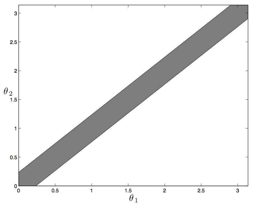
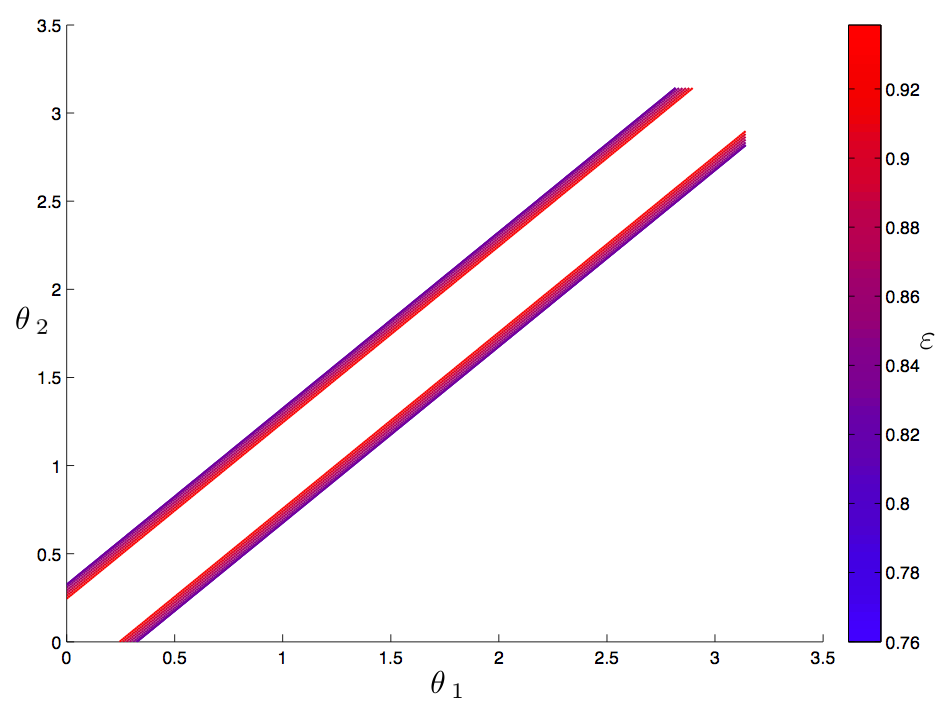
Figure 1. (a): The region of attraction for a special choice of admissible $\varepsilon$. (b): The boundary of region of attraction depending on $\varepsilon$.

4.2. Varying $D_{0}$

In Fig. 2, we try to illustrate the estimated region of attraction for different choices of constant $D_{0}\in(0,\pi)$, which needs to fit the condition (2.8). We choose 18 numbers in $(0,\pi)$:

$$\frac{\pi}{19},\,\frac{2\pi}{19},\,\frac{3\pi}{20},\,\dots,\frac{18\pi}{19},$$

and use the restriction (2.8) to find out the admissible ones. Simple computation indicates that all numbers in $[\frac{\pi}{19},\frac{9\pi}{19}]$ fit the condition (2.8). Then we carry out the simulation using the admissible ones. In view of Fig. 1, we choose $\varepsilon$ as the smallest one among the admissible choices of $\varepsilon$. Fig. 2 shows the result depending on the values of $D_{0}$, which indicates that the larger choice of $D_{0}$ produces a larger region.

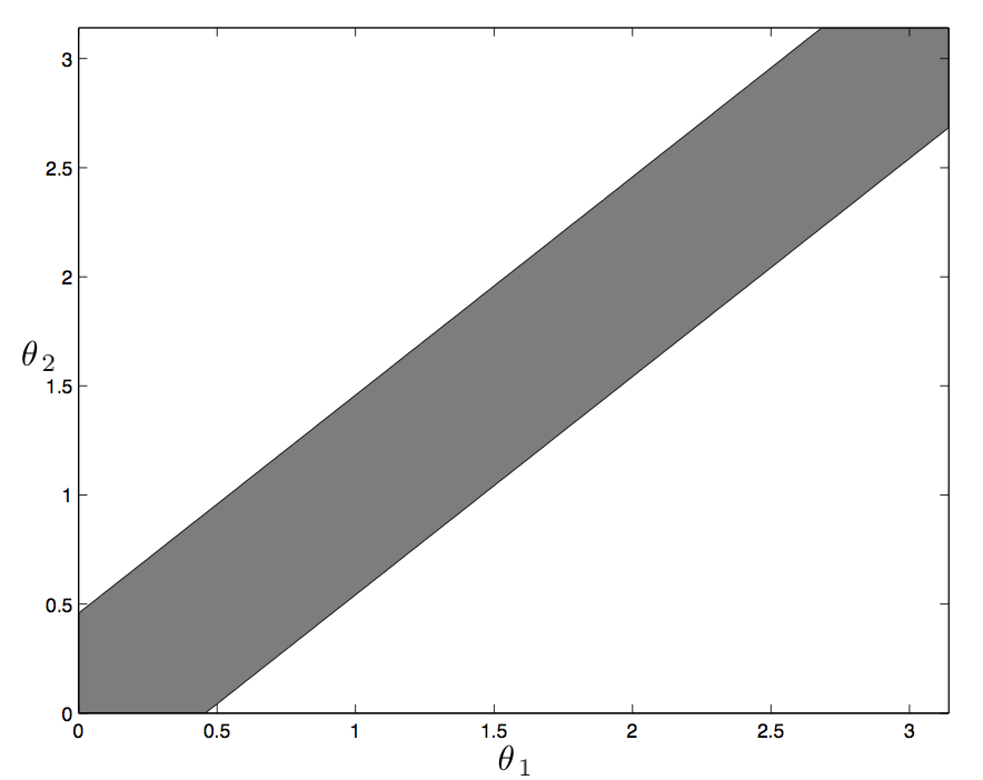
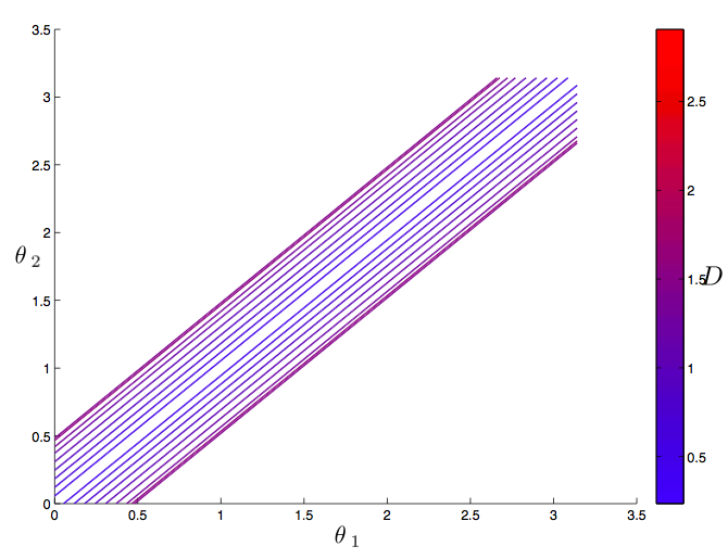
Figure 2. (a): The region of attraction for a special choice of admissible $D_{0}$. (b): The boundary of region of attraction depending on $D_{0}$.

4.3. Conservativeness

We acknowledge that our result is conservative in the sense that the framework is only sufficient for the phase locking behavior, for example, the presented estimate on the region of attraction. We do some simulations, see Fig. 3, to illustrate this. We use the same parameters as in the simulation for Fig. 1. For the initial phases, we chose $(\theta_{1},\theta_{2})=(3,1)$ which does not fit any region shown in Figs. 1-2. The employed numerical method is a classical fourth order Runge-Kutta one using the built-in ode45 Matlab command. The simulation in Fig. 3 shows that the frequencies are synchronized at an exponential rate, so the phase converges to a phase-locked state. This suggests a future problem to improve the estimate of the region of attraction.

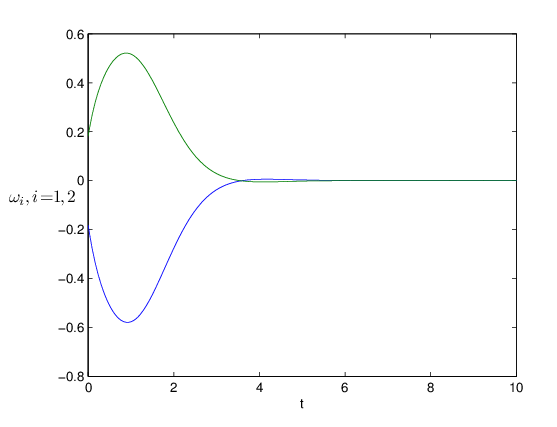
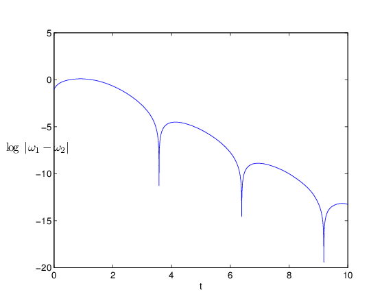
Figure 3. (a): The evolution of $\omega_{i},i=1,2$. (b): The evolution of $\log|\omega_{1}-\omega_{2}|$.

5. Conclusion

In this paper, we studied the synchronization and transient stability of the power grids on connected networks with inhomogeneous dampings. As mentioned before, the central problem for the transient stability is to identify the region of attraction of the synchronous states, which was considered actually very rare. In [22], a special case of the power network model was considered: the damping is homogeneous and the underlying graph has a diameter less than or equal to 2. This is very strict in real applications for power grids. Moreover, the analysis in [22], based on the phase diameter, heavily relied on these assumptions and cannot be extended to general cases. In the present work, we employed the energy method to overcome the difficulty and obtained the desired estimate for this problem in the general case. Simulations are provided to give some comparison on the different choices of parameters $D_{0}$ and $\varepsilon$, for a special setting of the simple network with two oscillators. In view of the potential application in engineering, the quantitative improvement of the estimate, including the parametric condition and the region of attraction, would be an interesting future problem. The heterogeneity of the parameters and/or general connectivity mean that the method of studying the phase difference cannot work well, while our estimate gives a way to overcome these difficulties. It is reasonable to expect a refined energy functional and a better energy estimate to improve the current result.

References

- [1] J. A. Acebron, L. L. Bonilla, C. J. P. Pérez Vicente, F. Ritort, and R. Spigler, The Kuramoto model: A simple paradigm for synchronization phenomena, Rev. Mod. Phys., 77 (2005), pp. 137-185.
- [2] H.-D. Chiang, Direct Methods for Stability Analysis of Electric Power Systems, Wiley, New York, 2011.
- [3] H.-D. Chiang, C. C. Chu, and G. Cauley, Direct stability analysis of electric power systems using energy functions: Theory, applications, and perspective, Proc. IEEE, 83 (1995), pp. 1497-1529.
- [4] H.-D. Chiang, F. F. Wu and P. P. Varaiya, Foundations of the potential energy boundary surface method for power system transient stability analysis, IEEE Trans. Circuits Systems, 35 (1988), pp. 712-728.
- [5] Y.-P. Choi, S.-Y. Ha, S. Jung, and Y. Kim, Asymptotic formation and orbital stability of phase-locked states for the Kuramoto model. Physica D, 241 (2012), pp. 735-754.
- [6] Y.-P. Choi, S.-Y. Ha, and S.-B. Yun, Complete synchronization of Kuramoto oscillators with finite inertia, Physica D, 240 (2011), pp. 32-44.
- [7] Y.-P. Choi, Z. Li, S.-Y. Ha, X. Xue, and S.-B. Yun, Complete entrainment of Kuramoto oscillators with inertia on networks via gradient-like flow, J. Diff. Eqs., 257 (2014), pp. 2591-2621.
- [8] N. Chopra, and M. W. Spong, On exponential synchronization of Kuramoto oscillators, IEEE Trans. Automatic Control, 54 (2009), pp. 353-357.
- [9] F. Dörfler, and F. Bullo, On the critical coupling for Kuramoto oscillators, SIAM. J. Appl. Dyn. Syst., 10 (2011), pp. 1070-1099.
- [10] F. Dörfler, and F. Bullo, Synchronization and transient stability in power networks and nonuniform Kuramoto oscillators, SIAM J. Control Optim., 50 (2012), pp. 1616-1642.
- [11] F. Dörfler, and F. Bullo, Synchronization in complex oscillator networks: A survey, Automatica, 50 (2014), pp. 1539-1564.
- [12] F. Dörfler, and F. Bullo, Kron reduction of graphs with applications to electrical networks, IEEE Trans. Circuits Systems I: Regular Papers, 60 (2013), pp. 150-163.
- [13] F. Dörfler, M. Chertkov, and F. Bullo, Synchronization in complex oscillator networks and smart grids, Proc. Natl. Acad. Sci., 110 (2013), pp. 2005-2010.
- [14] G. B. Ermentrout, An adaptive model for synchrony in the firefly Pteroptyx malaccae, J. Math. Biol., 29 (1991), pp. 571-585.
- [15] G. Filatrella, A. H. Nielsen, and N. F. Pedersen, Analysis of a power grid using a Kuramoto-like model, Eur. Phys. J. B, 61 (2008), pp. 485-491.
- [16] V. Fioriti, S. Ruzzante, E. Castorini, E. Marchei, and V. Rosato, Stability of a distributed generation network using the Kuramoto models, in Critical Information Infrastructure Security, Lecture Notes in Comput. Sci., Springer, New York, 2009, pp. 14-23.
- [17] A. Haraux, and M. A. Jendoubi, Convergence of solutions of second-order gradient-like systems with analytic nonlinearities, J. Diff. Eqs., 144 (1998), pp. 313-320 .
- [18] C. Huygens, Horologium Oscillatorium, Paris, France, 1673.
- [19] A. Jadbabaie, N. Motee, and M. Barahona, On the stability of the Kuramoto model of coupled nonlinear oscillators, Proceedings of the American Control Conference, Boston Massachusetts 2004.
- [20] Y. Kuramoto, International symposium on mathematical problems in mathematical physics, Lecture Notes Phys., 39 (1975), pp. 420.
- [21] Z. Li, X. Xue, and D. Yu, On the Łojasiewicz exponent of Kuramoto model, J. Math. Phys., 56 (2015), pp. 0227041:1-20.
- [22] Z. Li, X. Xue, and D. Yu, Synchronization and tansient stability in power grids based on Łojasiewicz inequalities, SIAM J. Control Optim., 52 (2014), pp. 2482-2511.
- [23] S. Łojasiewicz, Une propriété topologique des sous-ensembles analytiques réels, in Les Équations aux Dérivées Partielles, Éditions du Centre National de la Recherche Scientifique, Paris, 1963, pp. 87-89.
- [24] P. J. Menck, J. Heitzig, J. Kurths, and H. J. Schellnhuber, How dead ends undermine power grid stability, Nature Communications, 5 (2014), 3969.
- [25] A. Pikovsky, , M. Rosenblum, and J. Kurths, Synchrnization: A universal concept in nonlinear sciences, Cambridge University Press, Cambridge, 2001.
- [26] S. H. Strogatz, From Kuramoto to Crawford: exploring the onset of synchronization in populations of coupled oscillators, Physica D, 143 (2000), pp. 1-20.
- [27] P. W. Sauer and M. A. Pai, Power system dynamics and stability, Prentice-Hall, Englewood Cliffs, NJ, 1998.
- [28] D. Subbarao, R. Uma, B. Saha, and M. V. R. Phanendra, Self-organization on a power system, IEEE Power Engrg. Rev., 21 (2001), pp. 59-61.
- [29] J. L. van Hemmen, and W. F. Wreszinski, Lyapunov function for the Kuramoto model of nonlinearly coupled oscillators, J. Stat. Phys., 72 (1993), pp. 145-166.
- [30] P. Varaiya, F. F. Wu, and R. L. Chen, Direct methods for transient stability analysis of power systems: Recent results, Proc. IEEE, 73 (1985), pp. 1703-1715.
- [31] M. Verwoerd, and O. Mason, A convergence result for the Kuramoto model with all-to-all coupling, SIAM J. Appl. Dyn. Syst., 10 (2011), pp. 906-920.
- [32] M. Verwoerd, and O. Mason, Global Phase-Locking in Finite Populations of Phase-Coupled Oscillators, SIAM J. Appl. Dyn. Syst., 7 (2008), pp. 134-160.
- [33] J. B. Ward, Equivalent circuits for power-flow studies, Trans. Am. Inst. Electr. Eng. 68 (2009), pp. 373–382.
- [34] A.T. Winfree, Biological rhythms and the behavior of populations of coupled oscillators, J. Theor. Biol. 16 (1967), pp. 15–42.