Multi-wavelength study of the star-formation in the S237 H ii region

Abstract

We present a detailed multi-wavelength study of observations from X-ray, near-infrared to centimeter wavelengths to probe the star formation processes in the S237 region. Multi-wavelength images trace an almost sphere-like shell morphology of the region, which is filled with the 0.5–2 keV X-ray emission. The region contains two distinct environments - a bell-shaped cavity-like structure containing the peak of 1.4 GHz emission at center, and elongated filamentary features without any radio detection at edges of the sphere-like shell - where Herschel clumps are detected. Using the 1.4 GHz continuum and ¹²CO line data, the S237 region is found to be excited by a radio spectral type of B0.5V star and is associated with an expanding Hii region. The photoionized gas appears to be responsible for the origin of the bell-shaped structure. The majority of molecular gas is distributed toward a massive Herschel clump (M_clump $\sim$260 M_⊙), which contains the filamentary features and has a noticeable velocity gradient. The photometric analysis traces the clusters of young stellar objects (YSOs) mainly toward the bell-shaped structure and the filamentary features. Considering the lower dynamical age of the H ii region (i.e. 0.2-0.8 Myr), these clusters are unlikely to be formed by the expansion of the H ii region. Our results also show the existence of a cluster of YSOs and a massive clump at the intersection of filamentary features, indicating that the collisions of these features may have triggered cluster formation, similar to those found in Serpens South region.

1. Introduction

Massive stars ($\gtrsim$ 8 M_⊙) produce a flood of ultraviolet (UV) photons, radiation pressure, and drive strong winds, which allow them to interact with the surrounding interstellar medium (ISM). In star-forming regions, the radio and infrared observations have revealed the ring/shell/bubble/filamentary features surrounding the H ii regions associated with the OB stars, indirectly tracing the signatures of the energetics of powering sources (e.g. Deharveng et al., 2010; Watson et al., 2010; Dewangan et al., 2016). However, the physical processes of their interaction and feedback in their vicinity are still poorly understood (Zinnecker & Yorke, 2007; Tan et al., 2014). In recent years, with the availability of Herschel observations, the study of initial conditions of cluster formation toward the filaments, in particular, has received much attention in star formation research. However, the role of filaments in the formation of dense massive star-forming clumps and clusters is still a matter of debate (e.g. Myers, 2009; Schneider et al., 2012; Nakamura et al., 2014; Tan et al., 2014).

Located at a distance of 2.3 kpc (Pandey et al., 2013; Lim et al., 2015), the star-forming region, Sh 2-237 (hereafter S237; also known as NGC 1931/IRAS 05281+3412/RAFGL 5144/G173.9+0.3; $\alpha_{2000}$ = 05^h 31^m 22.8^s, $\delta_{2000}$ = +34$\arcdeg$ 13$\arcmin$ 59$\arcsec$) has a broken or incomplete ring or shell-like appearance at wavelengths longer than 2 $\mu$m (see Figure 1 in Pandey et al., 2013). One can find a comprehensive review of this star-forming region in Reipurth (2008). The H ii region associated with the S237 region (hereafter S237 H ii region) is ionized by a star of spectral type B0.5 (Glushkov et al., 1975) or two B2 main-sequence-type stars (Pandey et al., 2013). Balser et al. (2011) estimated the velocity of ionized gas to be about $-$0.64 km s^-1 in the S237 H ii region using a hydrogen radio recombination line (H87-93$\alpha$). Using CO (J = 1–0) line data, Yang et al. (2002) reported the radial velocity of molecular gas to be about $-$5.86 km s^-1 toward IRAS 05281+3412. Leisawitz et al. (1989) studied the molecular gas content of 34 open star clusters including S237 using ¹²CO (1-0) emission and suggested that a part of S237 is obscured by a molecular cloud. In the S237 region, Pandey et al. (2013) reported two separate stellar clusters and estimated a mean age of the young stellar objects (YSOs) to be 2$\pm$1 Myr. Based on the morphology of the region, ages of the YSOs and ionizing sources, they concluded a triggered star formation process in the S237 region. Using the isochrone fitting in the Hertzsprung-Russell diagram, Lim et al. (2015) reported a median age of 2 Myr with a spread of 4.5 Myr for the age distribution of the pre-main sequence (PMS) members in NGC 1931.

These previous studies suggest the presence of massive star(s) and ongoing star formation activity in the S237 region. The region is a relatively nearby star-forming site and has an interesting morphology, indicating it is a promising site to explore the impact of ionizing star(s). Despite the availability of different observational data-sets, the feedback of massive star(s) is not systematically studied in the S237 region. The physical conditions in the S237 region are yet to be determined and the velocity structure of molecular gas is also unknown. Recently, Herschel observations have revealed that filaments are often seen in the star-forming regions (e.g., Molinari et al., 2010; André et al., 2010). However, the identification of dense clumps and filaments is still lacking in the S237 region. Furthermore, the star formation toward clumps and filaments in S237 is yet to be probed. A knowledge of the physical environment of the region is very important to assess the ongoing physical mechanisms. In the present paper, we study in detail the physical processes responsible for the interaction and feedback effect of massive star(s) on its surroundings. To understand the ongoing physical mechanisms in S237, we examine the distribution of dust temperature, column density, extinction, ionized emission, hot gas, neutral hydrogen gas, kinematics of molecular gas, and YSOs using the multi-wavelength data.

In Section 2, we describe the multi-band data-sets used in the present work. In Section 3, we provide the details of results obtained. In Section 4, we discuss the possible star formation scenario based on our findings. Finally, the results are summarized and concluded in Section 5.

2. Data and analysis

In the present work, we selected a region of $\sim$30$\farcm 6$ $\times$ 30$\farcm 6$ (central coordinates: $l$ = 173$\arcdeg$.993; $b$ = 0$\arcdeg$.273) around the S237 region. In the following, a brief description of the multi-wavelength data spanning from X-ray, optical H$\alpha$, near-infrared (NIR) to radio wavelengths is presented.

2.1. X-ray data

The ROSAT 0.5–2 keV X-ray image was obtained from the public archives (observation ID: WG931113P_N1_SI01.N1) maintained at the High Energy Astrophysics Science Archive Research Center (HEASARC) in USA. The pixel scale of the image is 45$\arcsec$. One can obtain more details about the ROSAT observations in Voges et al. (1999). A single ROSAT source (i.e., J053134.4+341242; Voges et al., 2000) is found in the S237 region. In the catalog, the total X-ray count was reported with an extraction radius of 300$\arcsec$ (Voges et al., 1999), indicating the presence of an extended diffuse X-ray emission.

2.2. H$\alpha$ Narrow-band Image

Narrow-band H$\alpha$ image at 0.6563 $\mu$m was obtained from the Isaac Newton Telescope Photometric H$\alpha$ Survey of the Northern Galactic Plane (IPHAS; Drew et al., 2005) survey database. The survey was made using the Wide-Field Camera (WFC) at the 2.5-m INT, located at La Palma. The WFC consists of four 4k $\times$ 2k CCDs, in an L-shape configuration. The pixel scale is $0\farcs 33$ and the instantaneous field is about 0.3 square degrees. One can find more details about the IPHAS survey in Drew et al. (2005).

2.3. NIR (1–5 $\mu$m) Data

NIR photometric JHK magnitudes of point sources have been obtained from the UKIDSS Galactic Plane Survey (GPS; Lawrence et al., 2007) sixth archival data release (UKIDSSDR6plus) and the Two Micron All Sky Survey (2MASS; Skrutskie et al., 2006). Note that the UKIDSS GPS data are not available for the entire selected region and are available only for the zone-I area as highlighted by a dotted-line in Figure 1b. Hence, 2MASS data are employed for the area where UKIDSS GPS observations are absent. The UKIDSS observations (resolution $\sim$$0\farcs 8$) were taken using the UKIRT Wide Field Camera (WFCAM; Casali et al., 2007). The UKIDSS GPS photometric data were calibrated using the 2MASS data. We obtained only reliable UKIDSS GPS photometric data, following the conditions listed in Lucas et al. (2008) and Dewangan et al. (2015). 2MASS data were also retrieved for bright sources that were saturated in the GPS catalog. To obtain reliable 2MASS photometric data, only those sources from the 2MASS catalog are chosen for the study that have photometric magnitude error of 0.1 and less in each band.

Warm-Spitzer IRAC 3.6 and 4.5 $\mu$m photometric images (resolution $\sim$2$\arcsec$) and magnitudes of point sources have been retrieved from the Glimpse360 (Whitney et al., 2011) survey. The photometric magnitudes were obtained from the GLIMPSE360 highly reliable catalog. To obtain further reliable Glimpse360 photometric data, only those sources are selected that have photometric magnitude error of 0.2 and less in each band.

2.4. Mid-infrared (12–22 $\mu$m) Data

We utilized the publicly available archival WISE (Wright et al., 2010) images at mid-infrared (MIR) 12 $\mu$m (spatial resolution $\sim$6$\arcsec$) and 22 $\mu$m (spatial resolution $\sim 12\arcsec$). WISE photometric sensitivity is reported to be 0.86 and 5.4 mJy (11.3 and 8.0 Vega mag) at 12 and 22 $\mu$m, respectively, in unconfused regions on the ecliptic plane. Saturation affects photometry for objects brighter than approximately 3.8 and -0.4 mag at 12 and 22 $\mu$m, respectively.

2.5. Far-infrared and Sub-millimeter Data

Far-infrared (FIR) and sub-millimeter (sub-mm) continuum images were downloaded from the Herschel Space Observatory data archives. The processed level2_-5 images at 70 $\mu$m, 160 $\mu$m, 250 $\mu$m, 350 $\mu$m, and 500 $\mu$m were obtained using the Herschel Interactive Processing Environment (HIPE, Ott, 2010). The beam sizes of the Herschel images at 70 $\mu$m, 160 $\mu$m, 250 $\mu$m, 350 $\mu$m, and 500 $\mu$m are 5$\farcs$8, 12$\arcsec$, 18$\arcsec$, 25$\arcsec$, and 37$\arcsec$, respectively (Poglitsch et al., 2010; Griffin et al., 2010). In this work, Herschel continuum images are utilized to compute the Herschel temperature and column density maps of the S237 region. Following the method described in Mallick et al. (2015), we obtained the Herschel temperature and column density maps from a pixel-by-pixel spectral energy distribution (SED) fit with a modified blackbody to the cold dust emission in the Herschel 160–500 $\mu$m wavelengths (also see Dewangan et al., 2015). The Herschel 70 $\mu$m data are not used in the analysis, because the 70 $\mu$m emission is dominated by the UV-heated warm dust. In the following, a brief step-by-step description of the procedures is described.

The Herschel 160 $\mu$m image is calibrated in the unit of Jy pixel^-1, while the images at 250–500 $\mu$m are calibrated in the surface brightness unit of MJy sr^-1. The plate scales of the 160, 250, 350, and 500 $\mu$m images are 6.4, 6, 10, and 14 arcsec/pixel, respectively. In the first step, prior to the SED fit, the 160, 250, and 350 $\mu$m images were convolved to the lowest angular resolution of 500 $\mu$m image ($\sim$37$\arcsec$) and were converted into the same flux unit (i.e. Jy pixel^-1). Furthermore, these images were regridded to the pixel size of 500 $\mu$m image ($\sim$14$\arcsec$). These steps were carried out using the convolution kernels available in the HIPE software. Next, the sky background flux level was determined to be 0.051, 0.115, 0.182, and $-$0.0009 Jy pixel^-1 for the 500, 350, 250, and 160 $\mu$m images (size of the selected region $\sim$5$\farcm$6 $\times$ 7$\farcm$8; centered at: $l$ = 174$\arcdeg$.127; $b$ = $-$0$\arcdeg$.222), respectively. To avoid diffuse emission associated with the selected target, the featureless dark area away from the S237 region was carefully chosen for the background estimation.

Finally, to obtain the maps, we fitted the observed flux densities at each pixel with the modified blackbody model (see equations 8 and 9 given in Mallick et al., 2015). The fitting was done using the four data points for each pixel, retaining the dust temperature (T_d) and the column density ($N(\mathrm{H}_{2})$) as free parameters. In the analysis, we adopted a mean molecular weight per hydrogen molecule ($\mu_{H2}$=) 2.8 (Kauffmann et al., 2008) and an absorption coefficient ($\kappa_{\nu}$ =) 0.1 $(\nu/1000~{}{\rm GHz})^{\beta}$ cm² g^-1, including a gas-to-dust ratio ($R_{t}$ =) of 100, with a dust spectral index of $\beta$ = 2 (see Hildebrand, 1983). The final Herschel temperature and column density maps are presented in Section 3.3.

2.6. Molecular CO line data

The observations of ¹²CO(1-0) and ¹³CO(1-0) emission were taken using the Five College Radio Astronomy Observatory (FCRAO) 14 meter telescope in New Salem, Massachusetts. The FCRAO beam sizes are 45$\arcsec$ (with angular sampling of 22$\farcs$5) and 46$\arcsec$ (with angular sampling of 22$\farcs$5) for ¹²CO and ¹³CO, respectively. Each line data have a velocity resolution of 0.25 km s^-1. Typical rms values for the spectra are 0.25 K for ¹²CO and 0.2 K for ¹³CO (e.g. Heyer et al., 1996). The S237 region was observed as part of the Extended Outer Galaxy Survey (E-OGS, Brunt, 2004), that extends the coverage of the FCRAO Outer Galaxy Survey (OGS, Heyer et al., 1998) to Galactic longitude ($l$) = 193$\arcdeg$, over a Galactic latitude ($b$) range of $-$3$\arcdeg$.5 $\leq$ $b$ $\leq$ +5$\arcdeg$.5. These ¹²CO and ¹³CO data cubes were provided by M. Heyer and C. Brunt (through private communication). The FCRAO ¹²CO profile along the line of sight to the S237 region shows a single velocity component at v = $-$4.6 km s^-1.

2.7. Radio continuum data

Radio continuum map at 1.4 GHz was retrieved from the NRAO VLA Sky Survey (NVSS) archive. The survey covers the sky north of $\delta_{2000}$ = $-$40$\arcdeg$ at 1.4 GHz with a beam of 45$\arcsec$ and a nearly uniform sensitivity of $\sim$0.45 mJy/beam (Condon et al., 1998).

2.8. H i line data

21 cm H i line data were obtained from the Canadian Galactic Plane Survey (CGPS; Taylor et al., 2003). The velocity resolution of H i line data is 1.32 km s^-1, sampled every 0.82 km s^-1. The data have a spatial resolution of 1$\arcmin$ $\times$ 1$\arcmin$ csc$\delta$. The line data have a brightness-temperature sensitivity of $\Delta$T_B = 3.5 sin$\delta$ K. One can find more details about the CGPS observing and data processing strategy in Taylor et al. (2003).

3. Results

3.1. Multi-band picture of S237

3.1.1 Continuum emission and gas distribution in S237

The longer wavelength data enable to penetrate deeper into the star-forming cloud despite the high extinction, allowing to infer the physical environment of a given star-forming region. In this section, we employ multi-band data to trace the physical structure of the S237 region. Figure 1a shows a two-color composite image using Herschel 70 $\mu$m in red and WISE 12.0 $\mu$m in green. A three-color composite image (350 $\mu$m (red), 250 $\mu$m (green), and 22 $\mu$m (blue)) is shown in Figure 1b. The Herschel and WISE images depict a broken or incomplete ring or shell-like appearance of the S237 region at wavelengths longer than 2 $\mu$m. The images reveal a prominent bell-shaped cavity-like morphology and elongated filamentary features at the center and the edge of the shell-like structure, respectively (see Figures 1a and 1b). The inset on the bottom left shows the zoomed-in view around the IRAS 05281+3412 using the Spitzer 3.6 $\mu$m image (see Figure 1a). The filamentary features are also highlighted in the image. Figure 2 shows the radio continuum and molecular emissions overlaid on the Herschel image at 500 $\mu$m. The bulk of the 160–500 $\mu$m emission comes from cold dust components (see Section 3.3 for quantitative estimates), while the emission at 22 $\mu$m traces the warm dust emission (see Figure 1b). In Figure 2a, we show the spatial distribution of ionized emission traced in the NVSS 1.4 GHz map, concentrating near the bell-shaped cavity-like morphology. This also implies that the ionized emission is located within the shell-like structure. The radio continuum emission is absent toward the elongated filamentary features. In Figure 2b, we present the molecular ¹²CO (J = 1–0) gas emission in the direction of the S237 region, revealing at least four molecular condensations (designated as conds1-4). The ¹²CO profile traces the region in a velocity range between $-$7 and $-$2 km s^-1. The molecular condensations are also found toward the filamentary features and the bell-shaped cavity-like morphology. It can be seen that the majority of molecular gas is distributed toward the molecular condensation, conds1 where filamentary features are observed. The details of integrated ¹²CO map as well as kinematics of molecular gas are described in Section 3.4.

Together, Figures 1 and 2 have allowed us to obtain a pictorial multi-wavelength view of the environment in the S237 region.

3.1.2 Lyman continuum flux

In this section, we estimate the number of Lyman continuum photons using the radio continuum map which will allow to derive the spectral type of the powering candidate associated with the S237 H ii region. In Figure 2a, the NVSS radio map traces a spherical morphology of the S237 H ii region. We used the clumpfind IDL program (Williams et al., 1994) to estimate the integrated flux density and the radio continuum flux was integrated up to 0.3% contour level of peak intensity. Using the 1.4 GHz map, we computed the integrated flux density (S_ν) and radius (R_HII) of the H ii region to be 708 mJy and 1.27 pc, respectively. The integrated flux density allows us to compute the number of Lyman continuum photons (N_uv), using the following equation (Matsakis et al., 1976):

$$N_{uv}(s^{-1})=7.5\,\times\,10^{46}\,\left(\frac{S_{\nu}}{Jy}\right)\left(\frac{D}{kpc}\right)^{2}\left(\frac{T_{e}}{10^{4}K}\right)^{-0.45}\\ \times\,\left(\frac{\nu}{GHz}\right)^{0.1}$$ (1)

where S_ν is the measured total flux density in Jy, D is the distance in kpc, T_e is the electron temperature, and $\nu$ is the frequency in GHz. This analysis is performed for the electron temperature of 10000 K and a distance of 2.3 kpc. We obtain N_uv (or logN_uv) to be $\sim$2.9 $\times$ 10⁴⁷ s^-1 (47.47) for the S237 H ii region, which corresponds to a single ionizing star of spectral type B0.5V-B0V (see Table II in Panagia (1973) for a theoretical value).

The knowledge of N_uv and R_HII values is also used to infer the dynamical age (t_dyn) of the S237 H ii region. The age of the H ii region can be computed at a given radius R_HII, using the following equation (Dyson & Williams, 1980):

$$t_{dyn}=\left(\frac{4\,R_{s}}{7\,c_{s}}\right)\,\left[\left(\frac{R_{HII}}{R_{s}}\right)^{7/4}-1\right]$$ (2)

where c_s is the isothermal sound velocity in the ionized gas (c_s = 11 km s^-1; Bisbas et al. (2009)), R_HII is previously defined, and R_s is the radius of the Strömgren sphere (= (3 N_uv/4$\pi n^{2}_{\rm{0}}\alpha_{B}$)^1/3, where the radiative recombination coefficient $\alpha_{B}$ = 2.6 $\times$ 10^-13 (10⁴ K/T)^0.7 cm³ s^-1 (Kwan, 1997), N_uv is defined earlier, and “n₀” is the initial particle number density of the ambient neutral gas. Assuming typical value of n₀ (as 10³(10⁴) cm^-3), we calculated the dynamical age of the S237 H ii region to be $\sim$0.2(0.8) Myr.

3.2. IRAC ratio map and H i gas

To infer the signatures of molecular outflows and the impact of massive stars on their surroundings, the Spitzer-IRAC ratio maps have been employed in combination with the radio continuum emission (Povich et al., 2007; Watson et al., 2008; Dewangan & Anandarao, 2011; Dewangan et al., 2012, 2016). Due to almost identical point response function (PRF) of IRAC 3.6 $\mu$m and 4.5 $\mu$m images, a ratio map of 4.5 $\mu$m/3.6 $\mu$m emission can be obtained directly using the ratio of 4.5 $\mu$m to 3.6 $\mu$m images. IRAC 4.5 $\mu$m band harbors a hydrogen recombination line Br$\alpha$ (4.05 $\mu$m) and a prominent molecular hydrogen line emission ($\nu$ = 0–0 $S$(9); 4.693 $\mu$m), which can be excited by outflow shocks. IRAC 3.6 $\mu$m band contains polycyclic aromatic hydrocarbon (PAH) emission at 3.3 $\mu$m as well as a prominent molecular hydrogen feature at 3.234 $\mu$m ($\nu$ = 1–0 $O$(5)). The ratio map of 4.5 $\mu$m/3.6 $\mu$m emission is shown in Figure 3a, tracing the bright and dark/black regions. The shell-like morphology is depicted and the map traces the edges of the shell (see dark/black regions in Figure 3a). The 0.5–2 keV X-ray emission is detected within the shell-like morphology, indicating the presence of hot gas emission in the region (see Figure 3a). The prominent bell-shaped cavity and the elongated filamentary features are also seen in the ratio map (see arrows and highlighted dotted-dashed box in Figure 3a). In Figure 3b, the distribution of molecular gas, ionized gas, and hot gas emission is shown together. In ratio 4.5 $\mu$m/3.6 $\mu$m map, the bright emission regions suggest the domination of 4.5 $\mu$m emission, while the black or dark gray regions indicate the excess of 3.6 $\mu$m emission. In Figure 4, we present H$\alpha$ image overlaid with the NVSS 1.4 GHz and Herschel 70 $\mu$m emission. The H$\alpha$ image shows the extended diffuse H$\alpha$ emission in the S237 region which is well distributed within the shell-like morphology. Figure 4 also shows the spatial match between the H$\alpha$ emission and the radio continuum emission. Figures 5a and 5b show zoomed-in ratio map and color-composite image toward the radio peak. A bell-shaped cavity is evident and the peaks of radio continuum 1.4 GHz emission and diffuse H$\alpha$ emission are present within it (see Figures 4 and 5b). The warm dust emission traced in the 70 $\mu$m image depicts the walls of the bell-shaped cavity (see Figure 5b). However, the peak of molecular ¹²CO(1-0) emission does not coincide with the radio continuum peak (see Figure 5). This indicates that the bell-shaped cavity can be originated due to the impact of ionized emission (also see Section 3.6). In the ratio map, there are bright emission regions near the radio continuum emission, indicating the excess of 4.5 $\mu$m emission. As mentioned above, the 4.5 $\mu$m band contains Br$\alpha$ feature at 4.05 $\mu$m. Hence, due to the presence of ionized emission, these bright emission regions probably trace the Br$\alpha$ features. In Figure 5a, the excess of 4.5 $\mu$m emission is also observed to the bottom of the bell-shaped morphology, which is designated as subreg1 and is coincident with the 0.5–2 keV X-ray peak emission. We also find bright emission region near the elongated filamentary features where the radio continuum emission is absent (see arrows in Figure 3a). Hence, this emission is probably tracing the outflow activities. Considering the presence of 3.3 $\mu$m PAH feature in the 3.6 $\mu$m band, the edges of the shell-like morphology around the H ii region appear to depict photodissociation regions (or photon-dominated regions, or PDRs).

In Figure 6, we present 21 cm H i velocity channel maps of the S237 region. The bright H i feature is seen near the 1.4 GHz emission, however the sphere-like shell morphology is depicted in black or dark gray regions. It appears that the black or dark gray regions in the H i channel maps trace the H i self-absorption (HISA) features (i.e. shell-like HISA features) (e.g., Kerton, 2005). It has been suggested that the HISA features are produced by the residual amounts of very cold H i gas in molecular clouds (Burton et al., 1978; Baker & Burton, 1979; Burton & Liszt, 1981; Liszt et al., 1981). In the S237 region, the HISA features are more prominent in a velocity range of $-$2.29 to $-$3.11 km s^-1. The 21 cm H i line data are presented here only for a morphological comparison with the infrared images. The 0.5–2 keV X-ray emission is also shown in a channel map (at $-$2.29 km s^-1), allowing to infer the distribution of cold H i gas and hot gas emission in the region. In Figure 7, to compare the morphology of the S237 region, we have shown infrared images (at 22 $\mu$m and 250 $\mu$m) and H i map (at 21 cm). We find that the shell-like HISA feature is spatial correlated with dust emissions as traced in the Spitzer, WISE, and Herschel images. The presence of H i further indicates the PDRs surrounding the H ii region and hot gas emission.

3.3. Herschel temperature and column density maps

The Herschel temperature and column density maps are used to infer the physical conditions present in a given star-forming region. In Figure 8, we show the final temperature and column density maps (resolution $\sim$37$\arcsec$). The procedures for calculating the Herschel temperature and column density maps were mentioned in Section 2.5.

In the Herschel temperature map, the area near the H ii region is traced with the considerably warmer gas (T_d $\sim$29-47 K) (see Figure 8a). The Herschel temperature map traces the edges of the shell in a temperature range of about 22–28 K. Several condensations are found in the column density map and one of the condensations (see clump 1) has the highest column density (peak $N(\mathrm{H}_{2})$ $\sim$3.6 $\times$ 10²¹ cm^-2; A_V $\sim$3.8 mag) located toward the filamentary features (see Figure 8b). The relation between optical extinction and hydrogen column density ($A_{V}=1.07\times 10^{-21}~{}N(\mathrm{H}_{2})$; Bohlin et al., 1978) is used here. Krumholz & McKee (2008) proposed a threshold value of 1 gm cm^-2 (or corresponding column densities $\sim$3 $\times$ 10²³ cm^-2) for formation of massive stars. This implies that the formation of massive stars in the identified Herschel clumps is unlikely. The column density structure of the S237 appears non-homogeneous with higher column density clumps engulfed in a medium with lower column density. The bell-shaped cavity is also seen in the column density map.

In the column density map, we employed the clumpfind algorithm to identify the clumps and their total column densities. We find 13 clumps, which are labeled in Figure 8b and their boundaries are also shown in Figure 8c. Among 13 clumps, seven clumps (e.g., 1, 3, 4, 6, 7, 9, and 13) are found toward the edges of the shell-like structure, while other three clumps (e.g., 2, 5, and 11) are located within the shell-like structure and remaining three clumps (e.g., 8, 10, and 12) are away from the shell-like structure. To assess the spatial distribution of clumps with respect to the HISA features, these clumps are also marked in the CGPS 21 cm H i single-channel map at $-$3.94 km s^-1 (see Figure 6). The mass of each clump is computed using its total column density and can be determined using the formula:

$$M_{clump}=\mu_{H_{2}}m_{H}Area_{pix}\Sigma N(H_{2})$$ (3)

where $\mu_{H_{2}}$ is assumed to be 2.8, $Area_{pix}$ is the area subtended by one pixel, and $\Sigma N(\mathrm{H}_{2})$ is the total column density. The mass of each Herschel clump is tabulated in Table 1. The table also contains an effective radius of each clump, which is provided by the clumpfind algorithm. The clump masses vary between 10 M_⊙ and 260 M_⊙. The most massive clump (i.e. clump1) associated with the molecular condensation, conds1 (see Figure 2b) is away from the radio peak, while the clump2 linked with the molecular condensation, conds2 (see Figure 2b) is associated with the H ii region.

3.4. Kinematics of molecular gas

In this section, we present distributions of ¹²CO (J=1–0) and ¹³CO (J=1–0) gas in the S237 region. An inspection of the ¹²CO and ¹³CO line profiles reveals that the molecular cloud associated with the S237 region (i.e S237 molecular cloud) is well traced in a velocity range of $-$7 to $-$2 km s^-1. In general, ¹²CO emission is optically-thicker than ¹³CO. To study the spatial distribution of the molecular gas in the S237 region, in Figure 9, we present ¹²CO (J=1–0) velocity channel maps at different velocities within the velocity range from $-$6.25 to $-$1.75 km s^-1 in steps of 0.5 km s^-1. The channel maps show at least four molecular condensations (i.e. conds1–4) and the bulk of the molecular gas is found toward the condensation “conds1”. In Figure 10, we show the ¹³CO (J=1–0) velocity channel maps as zoomed-in view toward the condensation “conds1”, where the high- and low-velocity gas distribution is evident toward the Herschel clump1. Note that the molecular condensation, “conds1” contains the elongated filamentary features and a massive Herschel clump (i.e. clump1). In Figure 11, we present the integrated ¹²CO and ¹³CO intensity maps and the galactic position-velocity maps. In the position-velocity diagrams of the ¹²CO emission, we find a noticeable velocity gradient along the condensation “conds1” (see Figures 11c and 11e) and an almost inverted C-like structure (see Figure 11e). In Figure 11 (see right panels), we also show the integrated ¹³CO (1–0) intensity map and the position-velocity maps. The optical depth in ¹³CO is much lower than that in ¹²CO, and the ¹³CO data can trace dense region (n(H₂) $>$ 10³ cm^-3). The integrated ¹³CO intensity map detects only the condensation “conds1” which contains the Herschel clump1 (see Figure 8b). It suggests that the conds1 is the densest molecular condensations compared to other three condensations (i.e. conds2–4). Using the integrated ¹³CO intensity map (see Figure 11b), we compute the mass of the molecular condensation “conds1” to be about 242 M_⊙, which is in agreement with the clump mass estimated using the Herschel data. In the calculation, we use an excitation temperature of 20 K, the abundance ratio (N(H₂)/N(¹³CO)) of 7 $\times$ 10⁵, and the ratio of gas to hydrogen by mass of about 1.36. One can find more details about the clump mass estimation in Yan et al. (2016) (see equations 4 and 5 in Yan et al., 2016). The position-velocity diagrams of the ¹³CO emission clearly indicate the presence of a velocity gradient along the condensation “conds1” (see Figures 11d and 11f). The condensation “conds1” hosts a cluster of young populations (see Section 3.5.2) and filamentary features. Therefore, one can suspect the presence of molecular outflows in the condensation “conds1” (also see channel maps in Figure 10). The velocity gradient could also be explained as gas flowing through the filamentary features into their intersection. Due to the coarse beam of the FCRAO ¹²CO and ¹³CO data (beam size $\sim$45$\arcsec$), we do not further explore this aspect in this work and are also unable to infer the gas distribution toward the filamentary features.

Recently, based on the molecular line data analysis and modeling work, Arce et al. (2011) suggested an inverted C-like or ring-like structure for an expanding shell/bubble in the position-velocity diagrams (see Figure 5 in Arce et al. (2011)). In the S237 region, the presence of an inverted C-like structure in the position-velocity diagram can indicate an expanding shell. Additionally, as previously mentioned, the S237 H ii region is excited by a single source of radio spectral B0.5V. Hence, it appears that the S237 region is associated with an expanding H ii region with an expansion velocity of the gas to be $\sim$1.65 km s^-1.

All together, the FCRAO ¹²CO and ¹³CO data suggest the presence of the expanding H ii region.

3.5. Young stellar objects in S237

3.5.1 Identification of young stellar objects

The GLIMPSE360, UKIDSS-GPS, and 2MASS data allow us to investigate the infrared excess sources present in the S237 region. In the following, we describe the YSOs identification and classification schemes.

1. To identify infrared-excess sources, Gutermuth et al. (2009) described various conditions using the H, K, 3.6, and 4.5 $\mu$m data and utilized the dereddened color-color space ([K$-$[3.6]]₀ and [[3.6]$-$[4.5]]₀). Using the GLIMPSE360, UKIDSS-GPS, and 2MASS catalog, these dereddened colors were determined using the color excess ratios given in Flaherty et al. (2007). This dereddened color-color space is also used to identify possible dim extragalactic contaminants from YSOs with additional conditions (i.e., [3.6]₀ $<$ 15 mag for Class I and [3.6]₀ $<$ 14.5 mag for Class II). The observed color and the reddening laws (from Flaherty et al., 2007) are utilized to compute the dereddened 3.6 $\mu$m magnitudes. This scheme yields 80 (7 Class I and 73 Class II) YSOs (see Figure 12a).

2. We find that some sources have detections only in the H and K bands. To further select infrared excess sources from these selected population, we utilized a color-magnitude (H$-$K/K) diagram (see Figure 12b). The diagram depicts the red sources with H$-$K $>$ 0.65 mag. This color criterion is selected based on the color-magnitude analysis of the nearby control field. We identify 18 additional YSO candidates using this scheme in our selected region.

Using the UKIDSS, 2MASS, and GLIMPSE360 data, a total of 98 YSOs are obtained in the selected region. The positions of all YSOs are shown in Figure 13a.

3.5.2 Spatial distribution of YSOs

Using the nearest-neighbour (NN) technique, the surface density analysis of YSOs is a popular method to examine their spatial distribution in a given star-forming region (e.g. Gutermuth et al., 2009; Bressert et al., 2010; Dewangan et al., 2015), which can be used to find the young stellar clusters. Using the NN method, we obtain the surface density map of YSOs in a manner similar to that described in Dewangan et al. (2015) (also see equation in Dewangan et al., 2015). The surface density map of all the selected 98 YSOs was constructed, using a 5$\arcsec$ grid and 6 NN at a distance of 2.3 kpc. In Figure 13b, the surface density contours of YSOs are presented and are drawn at 3, 5, 7, 10, 15, and 20 YSOs/pc², increasing from the outer to the inner regions. In Figure 13b, two clusters of YSOs are observed in the S237 region and are mainly seen toward the Herschel clump1, clump2, and subreg1 (see Figure 13b). However, one cluster of YSOs seems to be linked with the Herschel clump2 and the subreg1 together. In Section 3.3, we have seen that the filamentary features and bell-shaped cavity are observed toward the Herschel clump1 and clump2, respectively. Hence, in the S237 region, the star formation activities are found toward the filamentary features, bell-shaped cavity, and subreg1 (see Figure 13b). Recently, Pandey et al. (2013) also identified young populations in the S237 region using the optical and NIR (1–5 $\mu$m) data. Based on the spatial distribution of young populations, they found most of the YSOs distributed mainly toward the bell-shaped cavity, subreg1, and filamentary features (see Figure 15 in Pandey et al., 2013), which was also reported by Lim et al. (2015) (see Figure 8 in Lim et al., 2015). Furthermore, Lim et al. (2015) found an elongated shape of the surface density contours of PMS sources which is very similar in morphology to that investigated in this work. Taken together, these previous results are in a good agreement with our presented results.

In the molecular condensation, conds1, the filamentary features are physically associated with a cluster of YSOs, a massive clump (having the highest column density, i.e. 3.6 $\times$ 10²¹ cm^-2), and molecular gas (see Figure 14). Interestingly, this result suggests the role of filaments in the star formation process.

3.6. feedback of a massive star

Based on the radio continuum data analysis, we find that the S237 region is powered by a radio spectral type of B0.5V star. To study the feedback of a massive star in its vicinity, we compute the three pressure components (i.e. pressure of an H ii region $(P_{HII})$, radiation pressure (P_rad), and stellar wind ram pressure (P_wind)) driven by a massive star. These pressure components ($P_{HII}$, P_rad, and P_wind) are defined below (e.g. Bressert et al., 2012):

$$P_{HII}=\mu m_{H}c_{s}^{2}\,\left(\sqrt{3N_{uv}\over 4\pi\,\alpha_{B}\,D_{s}^{3}}\right);\\$$ (4)

$$P_{rad}=L_{bol}/4\pi cD_{s}^{2};\\$$ (5)

$$P_{wind}=\dot{M}_{w}V_{w}/4\pi D_{s}^{2};\\$$ (6)

In the equations above, N_uv, c_s (= 11 km s^-1; in the ionized gas; Bisbas et al., 2009), and $\alpha_{B}$ are previously defined (see Section 3.1.2), $\mu$= 0.678 (in the ionized gas; Bisbas et al., 2009), m_H is the hydrogen atom mass, $\dot{M}_{w}$ is the mass-loss rate, V_w is the wind velocity of the ionizing source, L_bol is the bolometric luminosity of the source, and D_s is the projected distance from the location of the B0.5V star where the pressure components are estimated. The pressure components driven by a massive star are evaluated at D_s = 3.5 pc (i.e. the separation between the positions of the NVSS peak and clump1).

Adopting, $L_{bol}$ = 19952 L_⊙ (for a B0.5V star; Panagia, 1973), $\dot{M}_{w}$ = 2.5 $\times$ 10^-9 M_⊙ yr^-1 (for a B0.5V star; Oskinova et al., 2011), V_w = 1000 km s^-1 (for a B0.5V star; Oskinova et al., 2011) in the above equations, we compute P_HII $\approx$ 2.0 $\times$ 10^-11 dynes  cm^-2, $P_{rad}$ $\approx$ 1.7 $\times$ 10^-12 dynes  cm^-2, and P_wind $\approx$ 1.1 $\times$ 10^-14 dynes  cm^-2. The comparison of these pressure components indicates that the pressure of the H ii region is relatively higher than the radiation pressure and the stellar wind pressure. We also obtain the total pressure (P_total = P_HII + $P_{rad}$ + P_wind) driven by a massive star to be $\sim$2.2 $\times$ 10^-11 dynes  cm^-2. $P_{total}$ is comparable to the pressure associated with a typical cool molecular cloud ($P_{MC}$$\sim$10^-11–10^-12 dynes cm^-2 for a temperature $\sim$20 K and particle density $\sim$10³–10⁴ cm^-3) (see Table 7.3 of Dyson & Williams, 1980), suggesting that the clump1 is not destroyed by the impact of the ionized gas.

4. Discussion

In recent years, Spitzer and Herschel data have observed MIR shells or bubbles, infrared filaments, and young star clusters together in many massive star-forming regions, indicating the onset of numerous complex physical processes. The presence of bubbles/shells associated with H ii regions is often explained by the feedback mechanisms (such as ionizing radiation, stellar winds, and radiation pressure) of massive stars (e.g., Zinnecker & Yorke, 2007; Deharveng et al., 2010; Tan et al., 2014; Dewangan et al., 2015). The multi-band images have revealed an almost sphere-like shell morphology as the most prominent structure in the S237 region. The shell-like HISA feature surrounding the ionized emission is also seen in the 21 cm H i line data. The velocity structure of molecular gas has indicated the presence of an expanding H ii region associated with the S237 region (see Section 3.4). Additionally, in Section 3.6, based on the pressure calculations (P_HII, $P_{rad}$, and P_wind), we find that the photoionized gas linked with the S237 H ii region can be considered as the major contributor (against stellar winds and radiation pressure) for the feedback process in the S237 region. Hence, the presence of a bell-shaped cavity-like morphology could be explained by the impact of ionizing photons (see Section 3.2).

In Section 3.5.2, we detect only two clusters of YSOs in the S237 region. Thirteen Herschel clumps are identified in the S237 region and star formation activities are exclusively found toward the Herschel clump1 and clump2 (see Section 3.5.2). Interestingly, the clump1 and clump2 contain the bell-shaped cavity-like structure hosting the peaks of 1.4 GHz emission as well as diffuse H$\alpha$ emission and filamentary features without any radio continuum detection, respectively. Lim et al. (2015) also found two groups of PMS stars inferred using their surface density analysis and estimated a median age of PMS members to be 2.0 Myr. They also reported the maximum age difference between the stars in the these two groups to be about 0.7 Myr, on average. Considering the presence of the expanding H ii region, the spatial locations of the YSO clusters may indicate the triggered star formation scenario in the S237 region. One can obtain more details about different processes of triggered star formation in the review article by Elmegreen (1998). Evans et al. (2009) reported an average age of the Class I and Class II YSOs to be $\sim$0.44 Myr and $\sim$1–3 Myr, respectively. Comparing these typical ages of YSOs with the dynamical age of the S237 H ii region (i.e. $\sim$0.2–0.8 Myr; see Section 3.1.2), it seems that the S237 H ii region is too young for initiating the formation of a new generation of stars. It is also supported by the results obtained by Lim et al. (2015) (see above). Hence, the young clusters are unlikely to have been the product of triggered formation. The ¹³CO emission is not detected toward the clump2 and subreg1, indicating the absence of dense gas toward these subregions (see Figure 11b). Note that the hot gas emission is traced toward the subreg1 using the ROSAT X-ray image and is found away (about 2$\arcmin$) from the 1.4 GHz peak emission. The surface density contours are also seen toward the subreg1. We suspect that the diffuse X-ray emission could be originated from young stars present in the cluster (see subreg1 in Figure 5a). Due to coarse resolution of the ROSAT X-ray image, we cannot identify the X-ray-emitting young stars. In general, Elmegreen (2011) mentioned that open cluster complexes could be the remnants of star formation in giant clouds formed by gravitational instabilities in the Milky Way gas layer.

It is also worth mentioning that the Herschel clump1 is the most massive with about 260 M_⊙ and contains the filamentary features and has a noticeable velocity gradient in both the ¹²CO and ¹³CO emissions. In Figure 14, there is a convincing evidence for a physical association of a cluster of YSOs and a massive clump with the filamentary features, indicating the role of filaments in the star formation process. Recently, Nakamura et al. (2014) studied the filamentary ridges in the Serpens South Infrared dark cloud using the molecular line observations and argued that the filamentary ridges were appeared to converge toward the protocluster clump. Furthermore, they suggested the collisions of the filamentary ridges may have triggered cluster formation. Schneider et al. (2012) also carried out Herschel data analysis toward the Rosette Molecular Cloud and suggested that the infrared clusters were preferentially seen at the junction of filaments or filament mergers. They also reported that their outcomes are in agreement with the results obtained in the simulations of Dale & Bonnell (2011). In the present work, due to coarse beam sizes of the molecular line data, we cannot directly probe the converging of filaments toward the protocluster clump. Here, a protocluster clump is referred to a massive clump associated with a cluster of YSOs without any radio continuum emission. However, our results indicate the presence of a cluster of YSOs and a massive clump at the intersection of filamentary features, similar to those found in Serpens South region. Therefore, it seems that the collisions of these features may have influenced the cluster formation. Based on these indicative outcomes, further detailed investigation of this region is encouraged using high-resolution molecular line observations.

In general, the information of the relative orientation of the mean field direction and the filamentary features offers to infer the role of magnetic fields in the formation and evolution of the filamentary features. Using previous optical polarimetric observations (from Pandey et al., 2013), we find an average value of the equatorial position angle of three stars to be 161$\arcdeg$.5, which are located near the filamentary features (see the positions of these stars in Figure 14b), while the equatorial position angle of the filamentary features at their intersection zone is computed to be about 95$\arcdeg$. The polarization vectors of background stars indicate the magnetic field direction in the plane of the sky parallel to the direction of polarization (Davis & Greenstein, 1951). Hence, these filamentary features seem to be nearly perpendicular to the plane-of-the-sky projection of the magnetic field linked with the molecular condensation, conds1 in the S237 region, indicating that the magnetic field is likely to have influenced the formation of the filamentary features. Sugitani et al. (2011) studied NIR imaging polarimetry toward the Serpens South cloud and found that the magnetic field is nearly perpendicular to the main filament. In particular, the filamentary features in the S237 region appear to be originated by a similar process as observed in the Serpens South cloud. However, high-resolution polarimetric observations at longer wavelengths will be helpful to further explore the role of magnetic field in the formation of the filamentary features in the S237 region.

5. Summary and Conclusions

In order to investigate star formation processes in the S237 region, we have utilized multi-wavelength data covering from radio, NIR, optical H$\alpha$ to X-ray wavelengths. Our analysis has been focused on the molecular gas kinematics, ionized emission, hot gas, cold dust emission, and embedded young populations. Our main findings are as follows:

$\bullet$ The S237 region has a broken or incomplete ring or shell-like appearance at wavelengths longer than 2 $\mu$m and contains a prominent bell-shaped cavity-like morphology at the center, where the peak of the radio-continuum emission is observed. The elongated filamentary features are also seen at the edge of the shell-like structure, where the radio-continuum emission is absent.
$\bullet$ The distribution of ionized emission traced in the NVSS 1.4 GHz continuum map is almost spherical and the S237 H ii region is powered by a radio spectral type of B0.5V star. The dynamical age of the S237 H ii region is estimated to be $\sim$0.2(0.8) Myr for 10³(10⁴) cm^-3 ambient density.
$\bullet$ The molecular cloud associated with the S237 region (i.e. S237 molecular cloud) is well traced in a velocity range of $-$7 to $-$2 km s^-1. In the integrated ¹²CO map, at least four molecular condensations (conds1-4) are identified.
$\bullet$ In the integrated ¹³CO map, the molecular gas is seen only toward the condensation, conds1.
$\bullet$ Using 0.5–2 keV X-ray image, the hot gas emission is traced at the center of the shell-like morphology and could be due to young stars present in the cluster.
$\bullet$ The position-velocity analysis of ¹²CO emission depicts an inverted C-like structure, revealing the signature of an expanding H ii region with a velocity of $\sim$1.65 km s^-1.
$\bullet$ The pressure calculations (P_HII, $P_{rad}$, and P_wind) indicate that the photoionized gas associated with the S237 H ii region could be responsible for the origin of the bell-shaped structure seen in the S237 region.
$\bullet$ Thirteen Herschel clumps have been traced in the Herschel column density map. The majority of molecular gas is distributed toward a massive Herschel clump1 (M_clump $\sim$260 M_⊙), which contains the filamentary features. The position-velocity analysis of ¹²CO and ¹³CO emissions traces a noticeable velocity gradient along this Herschel clump1.
$\bullet$ The analysis of NIR (1–5 $\mu$m) photometry provides a total of 98 YSOs and also traces the clusters of YSOs mainly toward the bell-shaped structure and the filamentary features.
$\bullet$ Toward the elongated filamentary features, a cluster of YSOs is spatially coincident with a massive Herschel clump1 embedded within the molecular condensation, conds1.

Taking into account the lower dynamical age of the H ii region (i.e. 0.2-0.8 Myr), the clusters of YSOs are unlikely to be originated by the expansion of the H ii region. An interesting outcome of this work is the existence of a cluster of YSOs and a massive clump at the intersection of filamentary features, indirectly illustrating that the collisions of these features may have triggered cluster formation, similar to those seen in the Serpens South star-forming region.

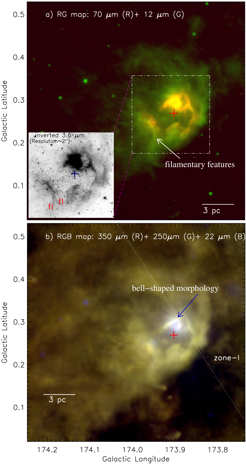
Figure 1.— Distribution of the MIR and sub-mm emissions toward the S237 region (size of the selected region $\sim$30$\farcm 6$ $\times$ 30$\farcm 6$ ($\sim$20.5 pc $\times$ 20.5 pc at a distance of 2.3 kpc); centered at $l$ = 173$\arcdeg$.993; $b$ = 0$\arcdeg$.273). a) Two color composite image (in logarithmic gray scale), which clearly illustrates the morphology of the region. The inset on the bottom left shows the central region in zoomed-in view, using the Spitzer 3.6 $\mu$m image (inverted gray scale; see a dotted-dashed white box in figure). Two filamentary features are highlighted by labels “fl”. b) Composite trichromatic image of the S237 region with the Herschel 350 $\mu$m, 250 $\mu$m, and WISE 22 $\mu$m bands in red, green, and blue, respectively. The UKIDSS GPS data are available only for the zone-I area as highlighted by a dotted-line. In both the panels, the position of IRAS 05281+3412 is marked by a plus (“+”) symbol. In both the panels, the scale bar corresponding to 3 pc (at a distance of 2.3 kpc) is shown in bottom-left. Figures reveal a shell-like morphology of the region, filamentary features, and a bell-shaped cavity-like structure.

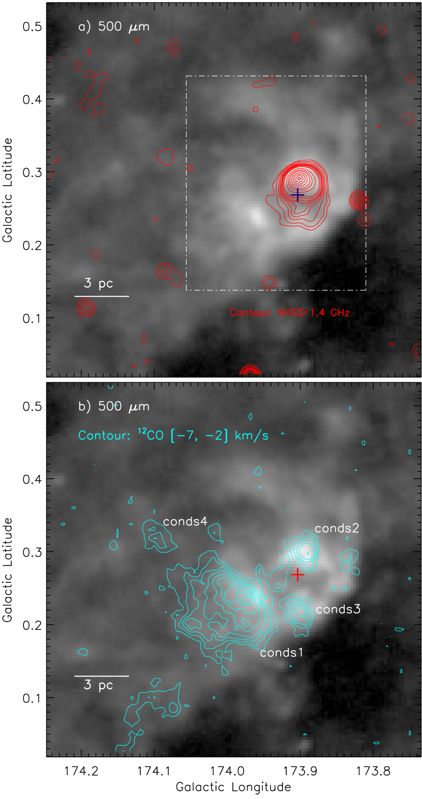
Figure 2.— Distribution of the sub-mm, ionized, and molecular emissions toward the S237 region. a) The radio continuum contours from the NVSS at 1.4 GHz are overlaid on the Herschel 500 $\mu$m image. The NVSS contours are superimposed with levels of 0.5, 1, 2, 3, 4, 5, 6, 8, 10, 20, 30, 40, 55, 70, 85, and 95% of the peak value (i.e., 0.1936 Jy/beam). The dotted-dashed white box encompasses the area shown in Figure 3a. b) The integrated ¹²CO (1–0) emission contours are overplotted on the Herschel 500 $\mu$m image. The ¹²CO emission contours are superimposed with levels of 1, 2, 3, 4, 55, 70, 80, 90, and 99% of the peak value (i.e., 36.5639 K km s^-1). In each panel, the scale bar at the bottom-left corner corresponds to 3 pc (at a distance of 2.3 kpc). In each panel, the marked symbol is similar to those shown in Figure 1. Figures show the distribution of ionized emission, molecular gas, and dense materials in the region.

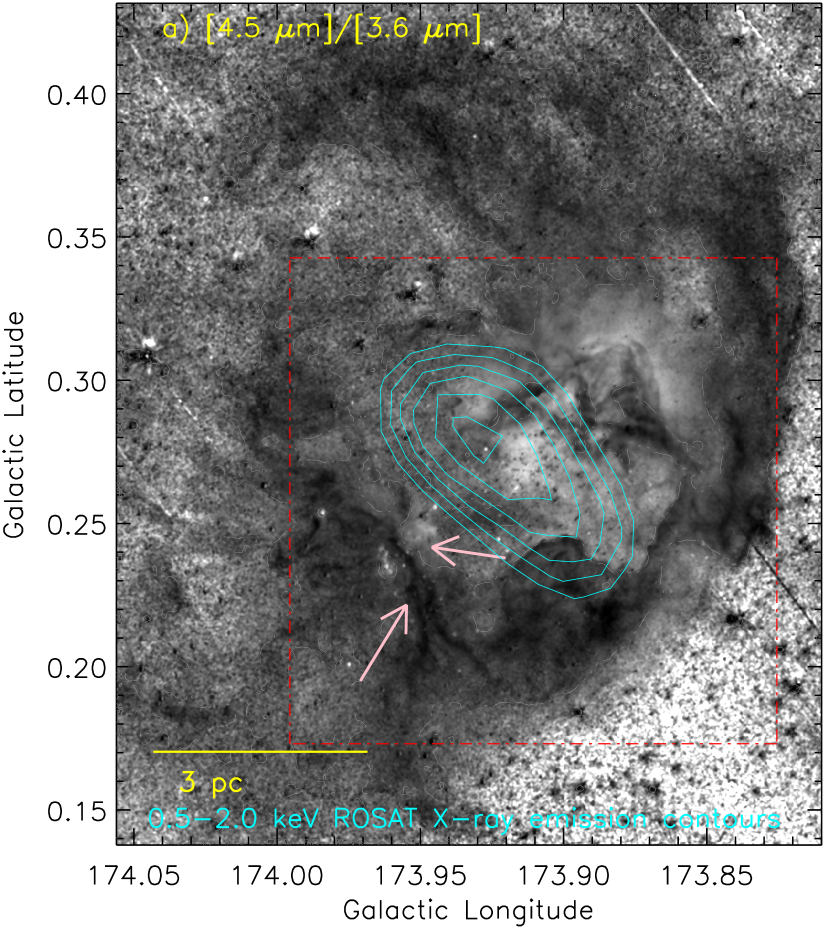
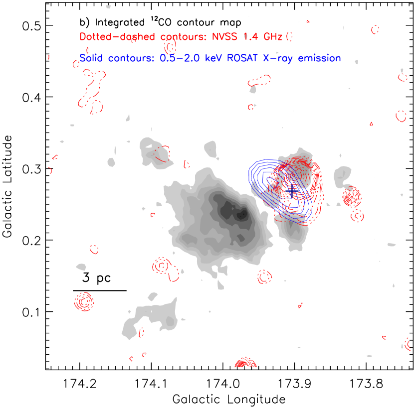
Figure 3.— a) Spitzer ratio map of 4.5 $\mu$m/3.6 $\mu$m emission. The ratio map is subjected to median filtering with a width of 5 pixels and smoothened by 4 pixel $\times$ 4 pixel using a boxcar algorithm. The dotted-dashed box (in red) encompasses the area shown in Figure 4. The 4.5 $\mu$m/3.6 $\mu$m emission contour (gray dotted-dashed contour) is also shown on the image with a representative value of 0.75, tracing the shell-like morphology. b) The contour map of integrated ¹²CO emission in the velocity range of $-$7 to $-$2 km s^-1. The contour levels are similar to the one shown in Figure 2b. The NVSS contours (red dotted-dashed contours) are also superimposed with similar levels to that shown in Figure 2a. The 0.5–2.0 keV ROSAT X-ray emission contours (solid contours) of S237 are overplotted on both the panels. The X-ray image is Gaussian smoothed with a radius of 3 pixels. In both the panels, the scale bar at the bottom-left corner corresponds to 3 pc (at a distance of 2.3 kpc).

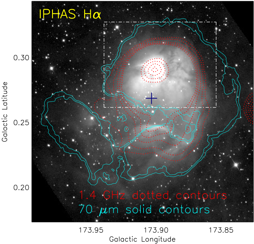
Figure 4.— IPHAS H$\alpha$ gray-scale image is overlaid with the NVSS 1.4 GHz and Herschel 70 $\mu$m emission contours. The NVSS 1.4 GHz dotted contours (in red) are shown with levels of 0.5, 1, 2, 3, 4, 55, 70, 85, and 95% of the peak value (i.e. 0.1936 Jy/beam). The dotted-dashed white box encompasses the area shown in Figures 5a and 5b.

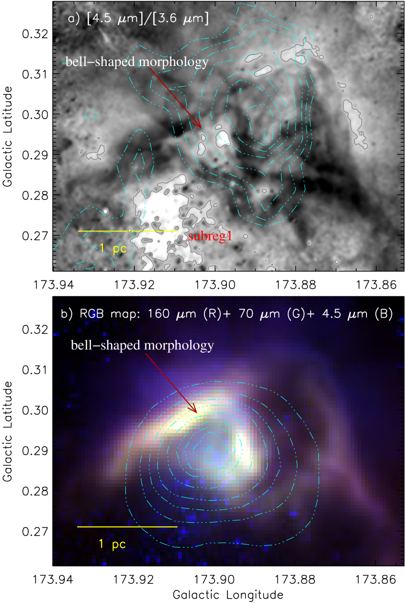
Figure 5.— a) Spitzer ratio map of 4.5 $\mu$m/3.6 $\mu$m emission is overlaid with the integrated ¹²CO (J = 1-0) contours. The ¹²CO contours are shown with levels of 20, 30, 40, 55, 70, 80, 90, and 99% of the peak value (i.e. 20.076 K km s^-1). The 4.5 $\mu$m/3.6 $\mu$m emission contour (in dark gray) is also shown on the image with a representative value of 0.99. b) Color-composite map using 160 $\mu$m (red), 70 $\mu$m (green), and 4.5 $\mu$m (blue) images. The map is overlaid with the NVSS 1.4 GHz contours. The NVSS 1.4 GHz contours are shown with levels of 10, 20, 30, 40, 55, 70, 80, 90, and 99% of the peak value (i.e. 0.1936 Jy/beam). In each panel, the scale bar at the bottom-left corner corresponds to 1 pc (at a distance of 2.3 kpc).

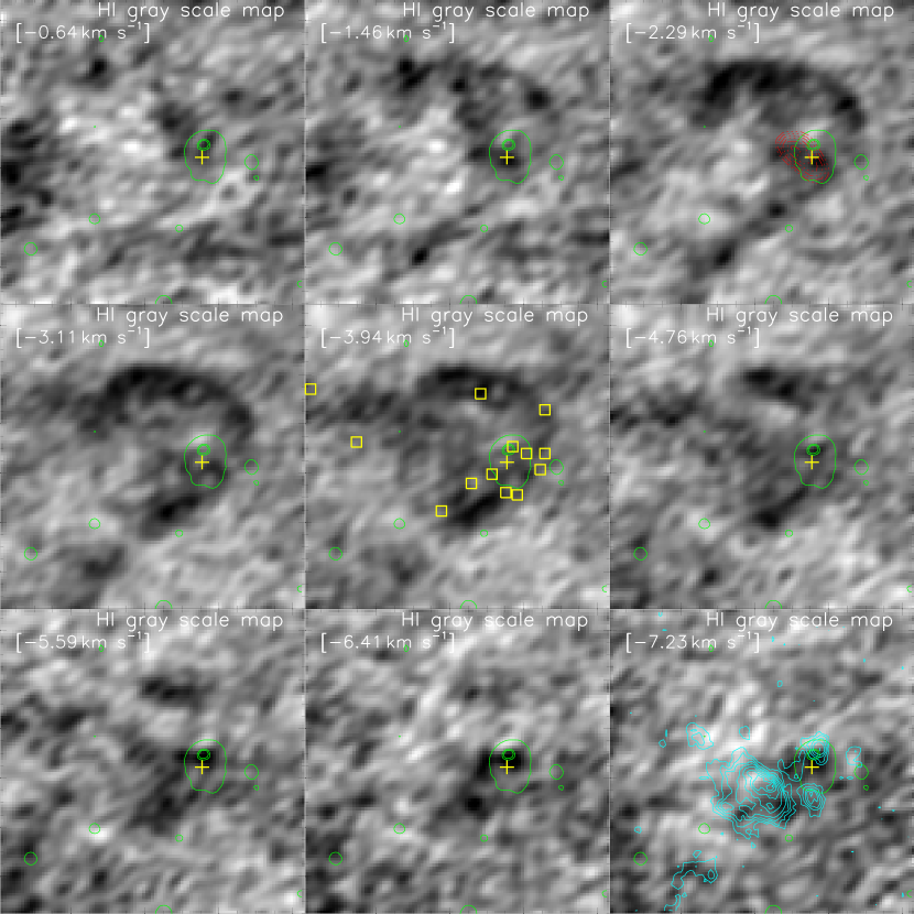
Figure 6.— The CGPS 21 cm H i velocity channel maps of the S237 region. The velocity value (in km s^-1) is labeled in each panel. In each panel, the NVSS 1.4 GHz contours (in green) are superimposed with levels of 1, 55, and 70% of the peak value (i.e., 0.1936 Jy/beam), tracing the ionized hydrogen emission. In each panel, the position of IRAS 05281+3412 is marked by a plus (“+”) symbol. In the third panel (at $-$2.29 km s^-1), the 0.5–2.0 keV ROSAT X-ray emission contours (red dotted-dashed contours) are similar to the one shown in Figure 3a. In the fifth panel (at $-$3.94 km s^-1), the identified Herschel clumps are marked by square symbols (in yellow; also see Figure 8b). To enhance the H i features, each channel map is smoothed with a boxcar average of 3 pixels width. In the last panel, the ¹²CO emission contours are similar to the one shown in Figure 2b. In the maps, the sphere-like shell morphology of the S237 region is revealed as H i self-absorption features (i.e., cold H i traced in absorption against warmer background H i; Kerton, 2005).

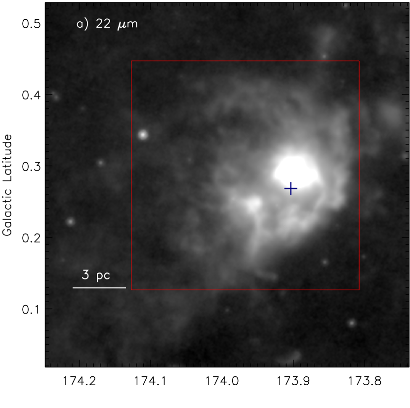
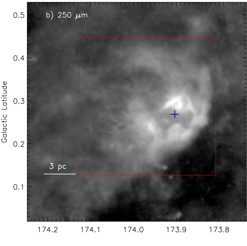
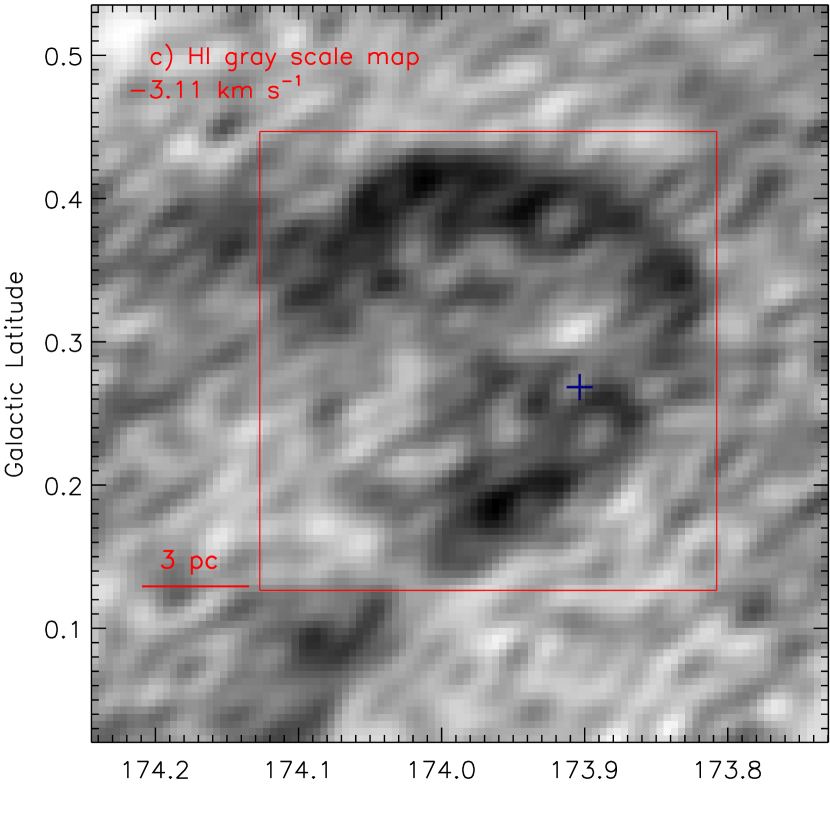
Figure 7.— Comparison of infrared images and H i map (at $-$3.11 km s^-1) of the S237 region. In each panel, a sold box (in red) shows an area where the shell-like morphology of the region is seen. In each panel, the scale bar at the bottom-left corner corresponds to 3 pc (at a distance of 2.3 kpc).

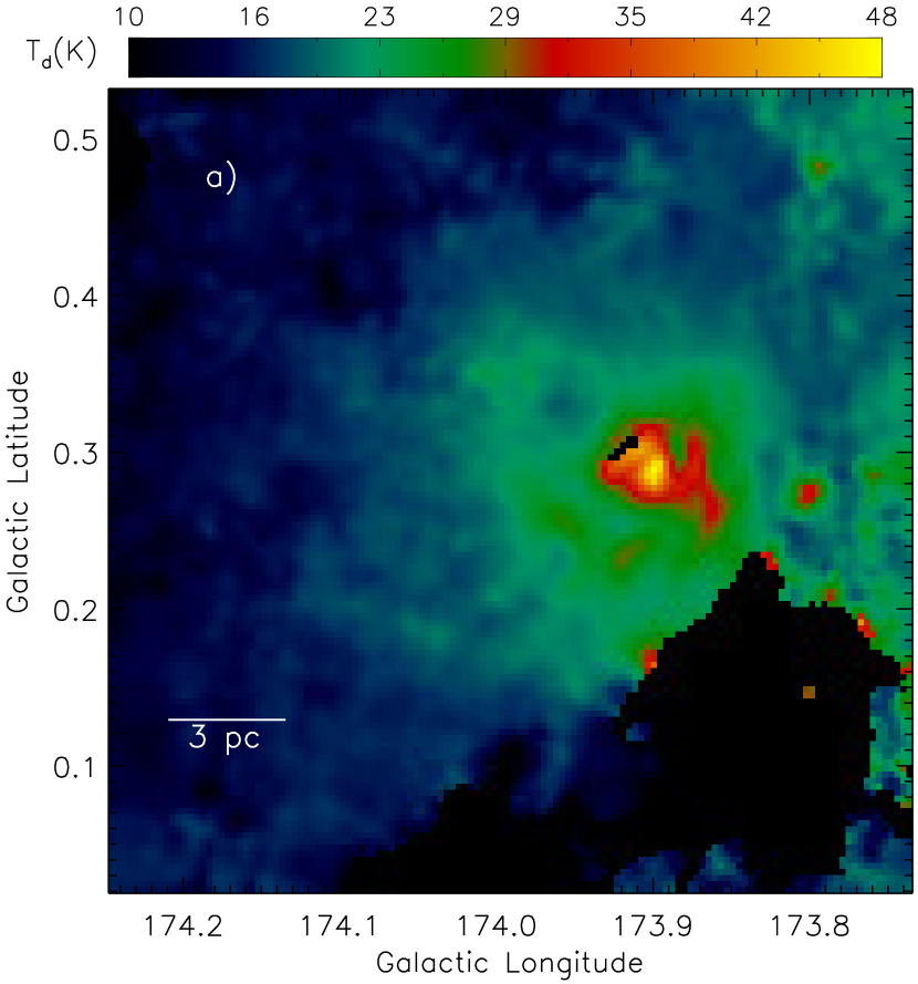
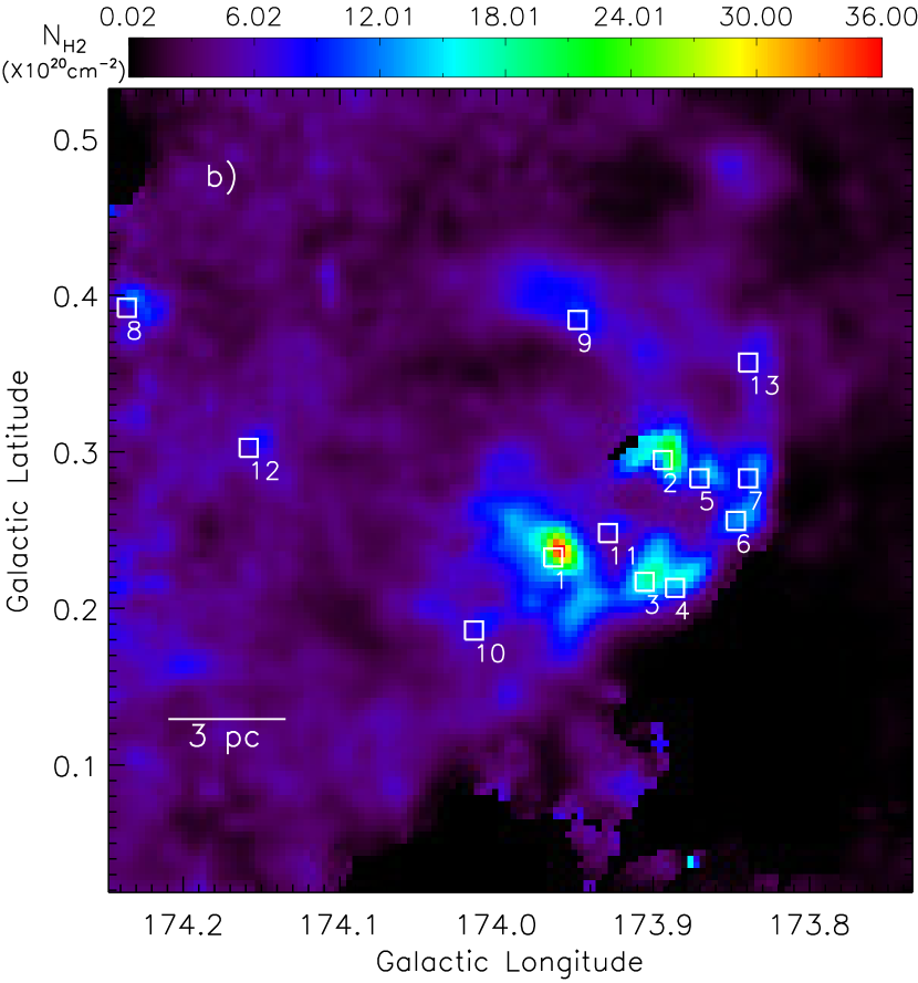
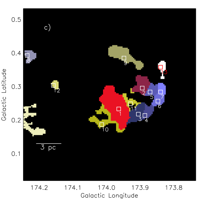
Figure 8.— Herschel temperature map (a) and column density ($N(\mathrm{H}_{2})$) map (b) of the region (see text for details). The column density map allows to infer the extinction with $A_{V}=1.07\times 10^{-21}~{}N(\mathrm{H}_{2})$ and to identify the clumps (see text for details). The identified clumps are marked by square symbols and the boundary of each identified clump is shown in Figure 8c (also see Table 1). c) The boundary of each identified clump is highlighted along with its corresponding clump ID (see Table 1 and also Figure 8b). In each panel, the scale bar at the bottom-left corner corresponds to 3 pc (at a distance of 2.3 kpc).

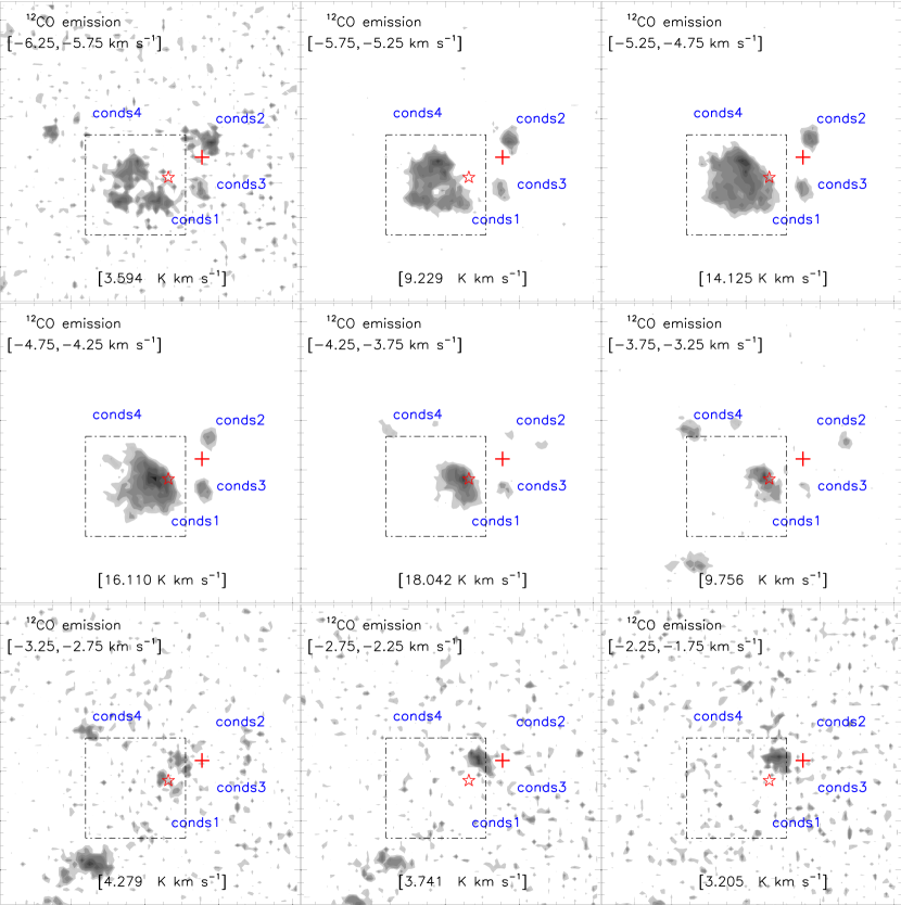
Figure 9.— Velocity channel contour maps of ¹²CO(J =1$-$0) emission. The molecular emission is integrated over a velocity interval, which is labeled in each panel (in km s^-1). The contour levels are 18, 25, 30, 40, 55, 70, 80, 90, and 99% of the peak value (in K km s^-1), which is also given in each panel. In each panel, the positions of IRAS 05281+3412 and Herschel column density peak are marked by a plus (“+”) and a star symbols, respectively. The dotted-dashed black box encompasses the area shown in Figures 10 and 14. In the maps, at least four noticeable condensations (i.e. conds1–4) are observed and the majority of molecular gas is found toward the condensation, conds1.

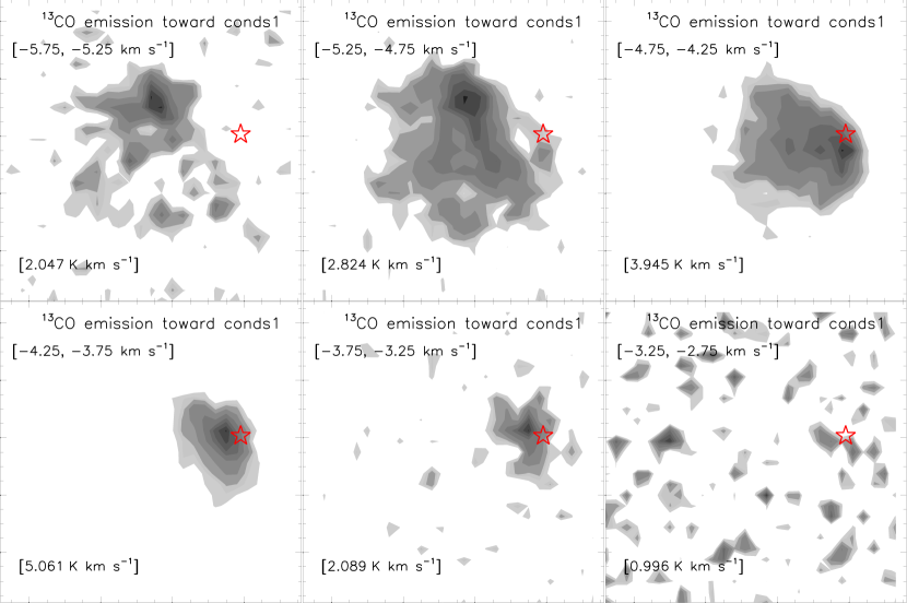
Figure 10.— The ¹³CO(J =1$-$0) velocity channel contour maps toward the molecular condensation, conds1 (see dotted-dashed black box in Figure 9). The molecular emission is integrated over a velocity interval, which is labeled in each panel (in km s^-1). The contour levels are 18, 25, 30, 40, 55, 70, 80, 90, and 99% of the peak value (in K km s^-1), which is also given in each panel. In each panel, the position of the Herschel column density peak is marked by a star symbol.

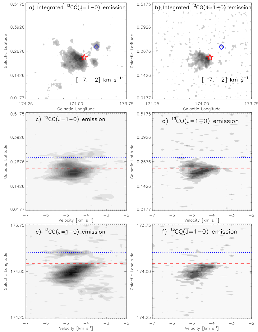
Figure 11.— The distribution of ¹²CO (left) and ¹³CO (right) emissions toward the S237 region. top panel: The contour maps of integrated ¹²CO (left; panel “a”) and ¹³CO (right; panel “b”) emissions in the velocity range of $-$7 to $-$2 km s^-1. The ¹²CO map is similar to the one shown in Figure 2b. In top panel, the positions of the NVSS 1.4 GHz peak emission and the Herschel column density peak are shown by a blue diamond and a red star, respectively. middle panel: The Latitude-velocity diagrams of ¹²CO (left; panel “c”) and ¹³CO (right; panel “d”). In the Latitude-velocity diagrams (panels “c” and “d”), the molecular emission is integrated over the longitude from 173$\arcdeg$.75 to 174$\arcdeg$.25. bottom panel: The Longitude-velocity diagrams of ¹²CO (left; panel “e”) and ¹³CO (right; panel “f”). In the Longitude-velocity diagrams (panels “e” and “f”), the molecular emission is integrated over the latitude from 0$\arcdeg$.0177 to 0$\arcdeg$.5175. In the position-velocity diagrams, the dotted blue and dashed red lines show the positions of the NVSS 1.4 GHz peak emission and the Herschel column density peak, respectively. In bottom left (panel “e”), the Longitude-velocity diagram depicts an inverted C-like morphology, indicating the expanding shell with an expanding gas velocity of $\sim$1.65 km s^-1. The position-velocity diagrams of ¹²CO and ¹³CO also trace a noticeable velocity gradient along the Herschel clump1, which contains the Herschel column density peak (also see the text).

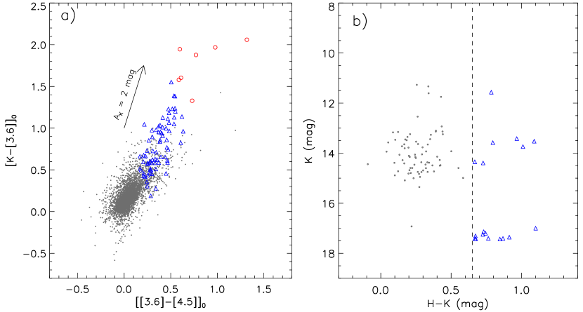
Figure 12.— Selection of embedded young stellar population within the region probed in this paper (see Figure 1). a) The dereddened [K$-$[3.6]]₀ $vs$ [[3.6]$-$[4.5]]₀ color-color diagram using the H, K, 3.6 $\mu$m, and 4.5 $\mu$m data. The extinction vector is drawn using the average extinction laws from Flaherty et al. (2007). b) Color-magnitude diagram (H$-$K/K) of the sources only detected in H and K bands that have no counterparts in our selected GLIMPSE360 catalog. In both the panels, Class I and Class II YSOs are marked by red circles and open blue triangles, respectively. In both the panels, the dots in gray color refer the stars with only photospheric emissions. The positions of all the identified YSOs are shown in Figure 13a.

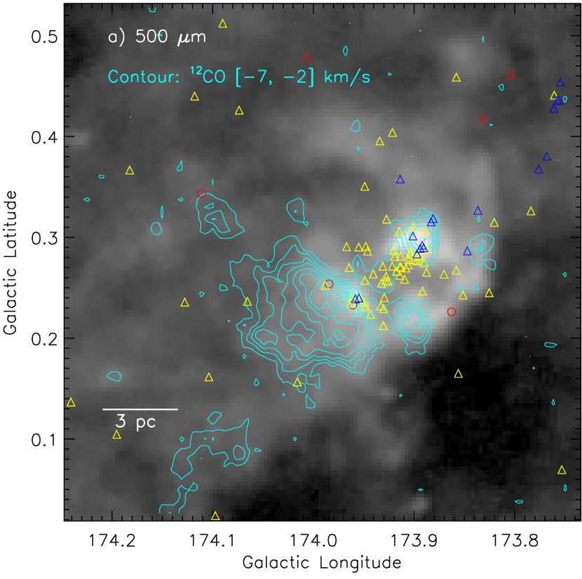
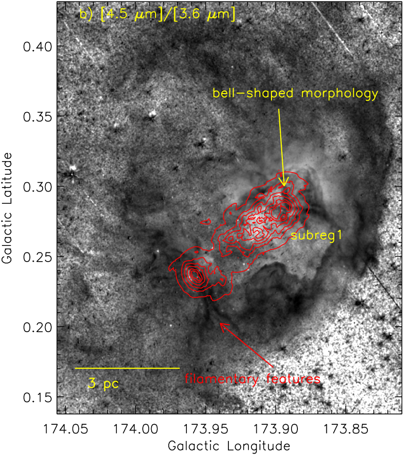
Figure 13.— The spatial distribution of YSOs identified within the region probed in this paper using the NIR (1–5 $\mu$m) data. a) The ¹²CO emission and the positions of YSOs are overlaid on the Herschel 500 $\mu$m map. The background map is similar to the one shown in Figure 2. The positions of Class I and Class II YSOs identified within our selected region are shown by circles (in red) and triangles (in blue and yellow), respectively. The YSOs selected using the H, K, 3.6 $\mu$m, and 4.6 $\mu$m data (see Figure 12a) are shown by red circles and yellow triangles, whereas the blue triangles represent the YSOs identified using the H and K bands (see Figure 12b). b) The surface density contours (in red) of all the identified YSOs are overlaid on the Spitzer-IRAC ratio map of 4.5 $\mu$m/3.6 $\mu$m emission (similar area as shown in Figure 3a), indicating the star formation activities mainly toward the filamentary features/clump1 and the bell-shaped morphology/clump2 (see text for details). The contours are shown at 3, 5, 7, 10, 15, and 20 YSOs/pc², from the outer to the inner side. In both the panels, the scale bar at the bottom-left corner corresponds to 3 pc (at a distance of 2.3 kpc).

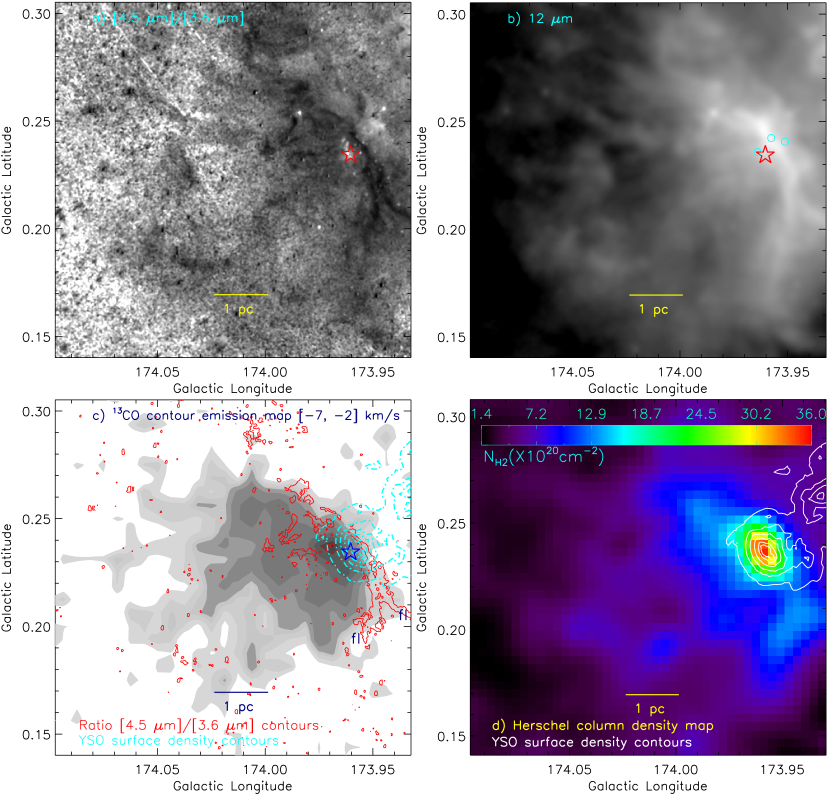
Figure 14.— Zoomed-in view toward the molecular condensation, conds1, as traced in the integrated ¹²CO and ¹³CO maps (see dotted-dashed box in Figure 9). a) Spitzer-IRAC ratio map of 4.5 $\mu$m/3.6 $\mu$m emission traces the filamentary features. b) WISE image at 12 $\mu$m also depicts the filamentary features. The positions of three stars having optical polarimetric observations (from Pandey et al., 2013) are marked by cyan circles. c) The integrated ¹³CO(J =1$-$0) emission map of the molecular condensation, conds1. The ¹³CO contours are shown with levels of 10, 18, 25, 30, 40, 55, 70, 80, 90, and 99% of the peak value (i.e. 8.251 K km s^-1). The YSO surface density contours (dotted dashed; in cyan color) and filamentary features (in red) are also shown in the map. Two filamentary features are highlighted by labels “fl”. d) Herschel column density map is overlaid with the YSO surface density contours, revealing a physical connection between a cluster of YSOs and a massive clump. In the last two panels, the contours are shown at 3, 5, 7, 10, 15, and 20 YSOs/pc², from the outer to the inner side. In the first three panels, the position of the Herschel column density peak is marked by a star symbol. Figures exhibit the presence of a cluster of YSOs and a massive clump at the intersection of filamentary features.

Table 1Summary of the properties of the Herschel clumps identified in the S237 region (see Figures 8b and 8c). Column 1 lists the IDs given to the clump. Table also contains positions, deconvolved effective radius (R_c), and clump mass (M_clump).

ID	l	b	Rc	Mclump
	[degree]	[degree]	(pc)	($M_{\odot}$)
1	173.9637	0.2325	1.8	258.6
2	173.8937	0.2947	1.0	84.3
3	173.9054	0.2169	1.0	80.2
4	173.8860	0.2130	0.7	37.4
5	173.8704	0.2830	0.7	35.2
6	173.8471	0.2558	0.7	36.0
7	173.8393	0.2830	0.6	25.0
8	174.2360	0.3919	0.7	27.6
9	173.9482	0.3842	1.3	85.7
10	174.0143	0.1858	1.1	60.4
11	173.9287	0.2480	0.7	24.1
12	174.1582	0.3025	0.5	11.7
13	173.8393	0.3569	0.6	18.5

References

- André et al. (2010) André, P., Men’shchikov, A., Bontemps, S., et al. 2010, A&A, 518, L102
- Arce et al. (2011) Arce, H. G., Borkin, M. A., Goodman, A. A., Pineda, J. E.,& Beaumont, C. N. 2011, ApJ, 742, 105
- Baker & Burton (1979) Baker, P., L., & Burton, W., B. 1979, A&AS, 35, 129
- Balser et al. (2011) Balser, D. S., Rood, R. T., Bania, T. M., & Anderson, L. D. 2011, ApJ, 738, 27
- Bisbas et al. (2009) Bisbas, T. G., Wünsch, R., Whitworth, A. P., & Hubber, D. A. 2009, A&A, 497, 649
- Bohlin et al. (1978) Bohlin, R. C., Savage, B. D., & Drake, J. F. 1978, ApJ, 224, 13233
- Bressert et al. (2010) Bressert, E., Bastian, N., Gutermuth, R., et al. 2010, MNRAS, 409, 54
- Bressert et al. (2012) Bressert, E., Ginsburg, A., Bally, J., et al. 2012, ApJ, 758, 28
- Brunt (2004) Brunt C., 2004, in Clemens D., Shah R., Brainerd T., eds, Proc. of ASP Conference 317. Milky Way Surveys: The Structure and Evolution of our Galaxy, p. 79
- Burton et al. (1978) Burton, W., B., Liszt, H., S., & Baker, P., L. 1978, ApJ, 219, 67
- Burton & Liszt (1981) Burton, W., B., & Liszt, H., S. 1981, in Origin of Cosmic Rays, eds. G. Setti, G. Spada, & A. W. Wolfendale, IAU Symp., 94, 227
- Casali et al. (2007) Casali, M., Adamson, A., Alves de Oliveira, C., et al. 2007, A&A, 467, 777
- Condon et al. (1998) Condon, J. J., Cotton, W. D., Greisen, E. W., et al. 1998, AJ, 115, 1693
- Dale & Bonnell (2011) Dale, J. E., & Bonnell, I. A. 2011, MNRAS, 414, 321
- Davis & Greenstein (1951) Davis, L., Jr., & Greenstein, J. L. 1951, ApJ, 114, 206
- Deharveng et al. (2010) Deharveng, L., Schuller, F., Anderson, L. D., et al. 2010, A&A, 523, 6
- Dewangan & Anandarao (2011) Dewangan, L. K., & Anandarao, B. G 2011, MNRAS, 414, 1526
- Dewangan et al. (2012) Dewangan, L. K., Ojha, D. K., Anandarao, B. G., Ghosh, S. K., & Chakraborti, S. 2012, ApJ, 756, 151
- Dewangan et al. (2015) Dewangan, L. K., Luna, A., Ojha, D. K., et al. 2015, ApJ, 811, 79
- Dewangan et al. (2016) Dewangan, L. K., Ojha, D. K., Luna, A., et al. 2016, ApJ, 819, 66
- Drew et al. (2005) Drew, J. E., Greimel, R., Irwin, M.J., et al. 2005, MNRAS, 362, 753
- Dyson & Williams (1980) Dyson, J. E., & Williams, D. A. 1980, Physics of the interstellar medium, New York, Halsted Press, 204 p
- Elmegreen (1998) Elmegreen, B. G. 1998, in ASP Conf. Ser. 148, Origins, ed. C. E. Woodward, J. M. Shull, & H. A. Thronson, Jr. (San Francisco, CA: ASP), 150
- Elmegreen (2011) Elmegreen, B., G. 2011, EAS Publications Series, EAS Publications Series, 51, 31
- Evans et al. (2009) Evans, N. J., II, Dunham, M. M., Jørgensen, J. K., et al. 2009, ApJS, 181, 321
- Flaherty et al. (2007) Flaherty, K. M., Pipher, J. L., Megeath, S. T., et al. 2007, ApJ, 663, 1069
- Glushkov et al. (1975) Glushkov, Y. I., Denisyuk, E. K., & Karyagina, Z. V. 1975, A&A, 39, 481
- Griffin et al. (2010) Griffin, M. J., Abergel, A., Abreu, A, et al. 2010, A&A, 518L, 3
- Gutermuth et al. (2009) Gutermuth, R. A., Megeath, S. T., Myers, P. C., et al. 2009, ApJS, 184, 18
- Heyer et al. (1996) Heyer, M. H., Carpenter, J. M., & Ladd, E. F. 1996, ApJ, 463, 630
- Heyer et al. (1998) Heyer, M., Brunt, C., Snell, R., et al. 1998, ApJS, 115, 241
- Hildebrand (1983) Hildebrand, R. H. 1983, Quarterly Journal of the RAS, 24, 267
- Kauffmann et al. (2008) Kauffmann, J., Bertoldi, F., Bourke, T. L., Evans, II, N. J.,& Lee, C. W. 2008, ApJ, 487, 993
- Kerton (2005) Kerton, C. R. 2005, ApJ, 623, 235
- Krumholz & McKee (2008) Krumholz, M., R., & McKee, C., F. 2008, Nature, 451, 1082
- Kwan (1997) Kwan, J. 1997, ApJ, 489, 284
- Lawrence et al. (2007) Lawrence, A., Warren, S. J., Almaini, O., et al. 2007, MNRAS, 379, 1599
- Leisawitz et al. (1989) Leisawitz, D., Bash, F. N., & Thaddeus, P. 1989, ApJS, 70, 731
- Lim et al. (2015) Lim, B., Sung, H., Hur, H., et al. 2015, JKAS, 48, 343
- Liszt et al. (1981) Liszt, H., S., Burton, W., B., & Bania, T., M. 1981, ApJ, 246, 74
- Lucas et al. (2008) Lucas, P. W., Hoare, M. G., Longmore, A., et al. 2008, MNRAS, 391, 1281
- Mallick et al. (2015) Mallick, K. K., Ojha, D. K., Tamura, M., et al. 2015, MNRAS, 447, 2307
- Matsakis et al. (1976) Matsakis, D. N., Evans, N. J., II, Sato, T., & Zuckerman, B. 1976, AJ, 81, 172
- Molinari et al. (2010) Molinari, S., Swinyard, B., Bally, J., et al., 2010, A&A, 518, L100
- Myers (2009) Myers, P. C. 2009, ApJ, 700, 1609
- Nakamura et al. (2014) Nakamura, F., Sugitani, K., Tanaka, T., et al 2014, ApJL, 791, L23
- Oskinova et al. (2011) Oskinova, L. M., Todt, H., Ignace, R., et al. 2011, MNRAS, 416, 1456
- Ott (2010) Ott, S. 2010, in Astronomical Society of the Pacic Conference Series, Vol. 434, Astronomical Data Analysis Software and Systems XIX, ed. Y. Mizumoto, K.-I. Morita, & M. Ohishi, 139
- Panagia (1973) Panagia, N. 1973, AJ, 78, 929
- Pandey et al. (2013) Pandey, A. K., Eswaraiah, C., Sharma, S. et al. 2013, ApJ, 764, 172
- Poglitsch et al. (2010) Poglitsch, A., Waelkens, C., Geis, N., et al. 2010, A&A, 518L, 2
- Povich et al. (2007) Povich, M. S., Stone, J. M., Churchwell, E., et al. 2007, ApJ, 660, 346
- Reipurth (2008) Reipurth, B., 2008, Handbook of Star Forming Regions Vol. I, Astronomical Society of the Pacific, Ed. B. Reipurth
- Schneider et al. (2012) Schneider, N., Csengeri, T., Hennemann, M., et al. 2012, A&A, 540, L11
- Skrutskie et al. (2006) Skrutskie, M. F., Cutri, R. M., Stiening, R., et al. 2006, AJ, 131, 1163
- Sugitani et al. (2011) Sugitani, K., Nakamura, F., Watanabe, M., et al. 2011, ApJ, 734, 63
- Tan et al. (2014) Tan, J. C., Beltrán, M. T., et al. 2014, aXriv 1402.0919
- Taylor et al. (2003) Taylor, A., R., Gibson, S., J., Peracaula, M., et al. 2003, AJ, 125, 3145
- Voges et al. (1999) Voges, W., Aschenbach, B., Boller, Th., et al. 1999, A&A, 349, 389
- Voges et al. (2000) Voges, W., Aschenbach, B., Boller, Th., et al. 2000, IAU Circ. 7432
- Watson et al. (2008) Watson, C., Povich, M. S., Churchwell, E. B., et al. 2008, ApJ, 681, 1341
- Watson et al. (2010) Watson, C., Hanspal, U., & Mensistu, A. 2010, ApJ, 716, 1478
- Whitney et al. (2011) Whitney, B., Benjamin, R., Meade, M., et al. 2011, Bulletin of the American Astronomical Society, Vol. 43
- Williams et al. (1994) Williams, J. P., de Geus, E. J., & Blitz, L. 1994, ApJ, 428, 693
- Wright et al. (2010) Wright, E. L., Eisenhardt, P. R. M., Mainzer, et al. 2010, AJ, 140, 1868
- Yan et al. (2016) Yan, Q. Z., Xu, Y., Zhang, B., et al. 2016, arXiv:1609.03051
- Yang et al. (2002) Yang, J., Jiang, Z., Wang, M., Ju, B., & Wang, H. 2002, ApJS, 141, 157
- Zinnecker & Yorke (2007) Zinnecker, H., & Yorke, H. W. 2007, ARA&A, 45, 481