Indistinguishable quantum walks on graphs relative to a bipartite quantum walker

Abstract

A distinguishability operator is defined for the continuous-time quantum walk (CTQW) of a bipartite quantum walker on two simply connected graphs, $W_{G_{i},G_{j}}=U_{G_{i}}\left(t\right)\otimes U_{G_{j}}\left(t^{\prime}\right)-U_{G_{j}}\left(t^{\prime}\right)\otimes U_{G_{i}}\left(t\right)$, where $U_{G_{i}}\left(t\right)$ is the unitary CTQW operator for a labeled graph $G_{i}$ over a time interval $t$. The null space of $W_{G_{i},G_{j}}$ defines the vector space of initial bipartite states whose time development is either constant or only dependent on $t+t^{\prime}$ and is invariant to which quantum walker subsystem goes with each graph. The set of null spaces corresponding with a set of $W_{G_{i},G_{j}}$ have interesting relations as subspaces, intersections between subspaces, and subspaces of intersections. These relations are depicted as Euler diagrams for labeled graphs of three and four vertices.

Keywords: Continuous-time quantum walk; Simply connected graph; Operator null space.

1 Introduction

Let $G=\left(V,E\right)$ be a simply connected and undirected labeled graph, where $V$ is a set of $n$ vertices and $E$ is a set of connecting edges. The adjacency matrix $A$ and degree matrix $D$ which describe the graph are defined as follows:

$$A_{j,k} =\begin{cases}1&\mbox{if there is an edge connecting vertices {j} and {k}}\\ 0&\mbox{otherwise}\end{cases}$$ (1a)

$$D_{j,k} =\begin{cases}deg\left(v_{j}\right)&\mbox{if }j=k\\ 0&\mbox{otherwise}\end{cases}$$ (1b)

where $deg\left(v_{j}\right)$ is the degree of vertex $v_{j}$.

Generally, the unitary CTQW operator $U_{G}(t)$ is defined in terms of the Laplacian matrix $L$ of the graph $G$. [1, 2]

$$L =D-A$$ (2a)

$$U_{G}\left(t\right) =e^{-itL}.$$ (2b)

The quantum walker is described by a time-dependent quantum state $\lvert\phi\left(t\right)\rangle$. The initial state vector $\lvert\phi\left(0\right)\rangle$ is an ordered set of components, each component corresponding to the initial amplitude at each vertex of the graph (we will label each vertex starting with $0$)

$$\lvert\phi\left(0\right)\rangle=\left(\phi_{0}\left(0\right),\phi_{1}\left(0\right),\phi_{2}\left(0\right),...,\phi_{n-1}\left(0\right)\right)$$ (3)

such that

$$\langle\phi\left(0\right)\lvert\phi\left(0\right)\rangle=\displaystyle\sum_{j=0}^{n-1}\left\lvert\phi_{j}\left(0\right)\right\rvert^{2}=1.$$ (4)

The time development of the quantum walk then becomes

$$U_{G}\left(t\right)\lvert\phi\left(0\right)\rangle=\lvert\phi\left(t\right)\rangle,$$ (5)

and the time-dependent amplitude at vertex $j$ is

$$\phi_{j}\left(t\right)=\langle j\lvert\phi\left(t\right)\rangle$$ (6)

such that after a time evolution of $t=t_{f}$ the probability for observing the walker at vertex j is $\langle\phi_{j}\left(t_{f}\right)\lvert\phi_{j}\left(t_{f}\right)\rangle$.

2 The bipartite quantum walker on two graphs

For two quantum systems labeled $A$ and $B$ let $\mathcal{H}_{A}$ and $\mathcal{H}_{B}$ represent the Hilbert spaces for the state vectors $\lvert\psi\rangle_{A}$ and $\lvert\psi\rangle_{B}$ respectively. The Hilbert space for the composite system $A\cup B$ is then $\mathcal{H}_{AB}=\mathcal{H}_{A}\otimes\mathcal{H}_{B}$ and the composite state vector becomes

$$\lvert\psi\rangle_{AB} =\displaystyle\sum_{i,j}\alpha_{i,j}\lvert i\rangle_{A}\otimes\lvert j\rangle_{B},$$ (7a)

$$\displaystyle\sum_{i,j}\lvert\alpha_{i,j}\rvert^{2} =1,$$ (7b)

where $\lvert i\rangle_{A}$ and $|j\rangle_{B}$ are standard bases in $\mathcal{H}_{A}$ and $\mathcal{H}_{B}$ respectively.

A bipartite state vector which can be represented as $\lvert\psi\rangle_{AB}=\lvert\psi\rangle_{A}\otimes\lvert\psi\rangle_{B}$ is called a separable state, otherwise it is called an entangled state. Unitary operations which are separable on the subsystems $A$ and $B$ are of the form $U_{AB}=U_{A}\otimes U_{B}$.

Given two graphs $G_{1}=\left(V_{1},E_{1}\right)$ and $G_{2}=\left(V_{2},E_{2}\right)$ the composite CTQW operator will be

$$U_{G_{1},G_{2}}\left(t,t^{\prime}\right)=U_{G_{1}}\left(t\right)\otimes U_{G_{2}}\left(t^{\prime}\right),$$ (8)

where the quantum walk on graph $G_{1}$ ($G_{2}$) is for a time $t$ ($t^{\prime}$). Accordingly, the time evolution of an initial bipartite walker will be

$$U_{G_{1}}\left(t\right)\otimes U_{G_{2}}\left(t^{\prime}\right)\lvert\psi_{0}\rangle_{AB}=\lvert\psi\left(t,t^{\prime}\right)\rangle_{AB},$$ (9)

in which $U_{G_{1}}\left(t_{1}\right)$ acts on subsystem $A$ and $U_{G_{2}}\left(t_{2}\right)$ acts on subsystem $B$ and $\lvert\alpha_{i,j}\rvert^{2}$ from equations 7a and 7b is the joint probability for finding subsystems $A$ and $B$ at vertices $i$ and $j$ of graphs $G_{1}$ and $G_{2}$ respectively. The entropy of entanglement of $\lvert\psi_{0}\rangle_{AB}$ is invariant to the locally separable operator $U_{G_{1},G_{2}}\left(t,t^{\prime}\right)$ [3].

3 Indistinguishability relative to $\lvert\psi_{0}\rangle_{AB}$

For the bipartite walker on two graphs $G_{i}$ and $G_{j}$ we define a non-unitary distinguishability operator

$$W_{G_{i},G_{j}}=U_{G_{i}}\left(t\right)\otimes U_{G_{j}}\left(t^{\prime}\right)-U_{G_{j}}\left(t^{\prime}\right)\otimes U_{G_{i}}\left(t\right).$$ (10)

We are interested in the null space of $W_{G_{i},G_{j}}$, i.e., the space of walker initial states which satisfy

$$W_{G_{i},G_{j}}\lvert\psi_{0}\rangle_{AB}=0$$ (11)

with $t$ and $t^{\prime}$ greater than $0$. Any initial state $\lvert\psi_{0}\rangle_{AB}$ in the null space of $W_{G_{i},G_{j}}$ will have the property

$$U_{G_{i}}\left(t\right)\otimes U_{G_{j}}\left(t^{\prime}\right)\lvert\psi_{0}\rangle_{AB}=U_{G_{j}}\left(t^{\prime}\right)\otimes U_{G_{i}}\left(t\right)\lvert\psi_{0}\rangle_{AB}=\lvert\psi\left(t+t^{\prime}\right)\rangle_{AB}.$$ (12)

We point out that for any two graphs $G_{i}$ and $G_{j}$ a trivial solution to Equation 11 (in addition to the zero vector) is the uniform amplitude $\lvert\psi_{0}\rangle_{AB}=\dfrac{1}{\sqrt{d}}\left(1,1,...,1\right)$ where $d$ is the cardinality of $\mathcal{H}_{AB}$, $d=\lvert V_{G_{i}}\rvert\times\lvert V_{G_{j}}\rvert$.

We will consider the condition when $\lvert V_{G_{i}}\rvert=\lvert V_{G_{j}}\rvert$: the two simply connected graphs have equal order $n$. For the special case $i=j$ the two graphs are isomorphic and are labeled equivalently although the duration of the quantum walk may be different for each graph. In this case

$$\mathrm{null}\left(W_{G_{i},G_{i}}\right) =\mathrm{null}\left(U_{G_{i}}\left(t\right)\otimes I_{n}-I_{n}\otimes U_{G_{i}}\left(t\right)\right)=\mathrm{null}\left(L_{G_{i}}\otimes I_{n}-I_{n}\otimes L_{G_{i}}\right)$$ (13)

$$=\mathrm{null}\left(I_{n}\otimes U_{G_{i}}\left(t^{\prime}\right)-U_{G_{i}}\left(t^{\prime}\right)\otimes I_{n}\right)=\mathrm{null}\left(I_{n}\otimes L_{G_{i}}-L_{G_{i}}\otimes I_{n}\right),$$

where $I_{n}$ is the $n\times n$ identity matrix and $L_{G_{i}}$ is the Laplacian matrix of $G_{i}$ .

Solutions to 13 are more easily obtained through analysis of an equivalent expression: [4, 5].

$$\left(I_{n}\otimes L_{G_{i}}-L_{G_{i}}\otimes I_{n}\right)\lvert\psi_{0}\rangle_{AB}=0$$ (14)

$$\mathrm{is\>equlivalent\>to}$$

$$L_{G_{i}}X-XL_{G_{i}}=0,$$

where $X$ is a variable $n\times n$ matrix such that $\lvert\psi_{0}\rangle_{AB}=\mathrm{vec}(X)$, and every $L_{G_{i}}$ is symmetric.

When $i\neq j$, $G_{i}$ and $G_{j}$ may be non-isomorphic graphs or isomorphic graphs with different labeling. In either case the null space of $W_{G_{i},G_{j}}$ will be

$$\mathrm{null}\left(W_{G_{i},G_{j}}\right)\subseteq\mathrm{null}\left(W_{G_{i},G_{i}}\right)\cap\mathrm{null}\left(W_{G_{j},G_{j}}\right),$$ (15)

from which $\mathrm{null}\left(W_{G_{i},G_{j}}\right)$ can be determined by inspection.

The null space of $W_{Kn,Kn}$, where $Kn$ is the complete graph of order $n$, encompasses all other $\mathrm{null}\left(W_{G_{i},G_{j}}\right)$,

$$\mathrm{null}\left(W_{G_{i},G_{j}}\right)\subseteq\mathrm{null}\left(W_{Kn,Kn}\right),$$ (16)

and

$$\mathrm{null}\left(W_{G_{i},G_{i}}\right)=\mathrm{null}\left(W_{G_{i},Kn}\right).$$ (17)

We find that it is convenient to work with and describe the null space of $W_{G_{i},G_{j}}$ in a non-orthonormal basis in which the simple sum of the basis vectors is the uniform vector $\left(1,1,...,1\right)$. In the next section we illustrate how this works.

3.1 $\mathrm{null}\left(W_{G_{i},G_{j}}\right)$ for graphs of order 3

There are 4 different labeled graphs with order 3, see Fig. 1.

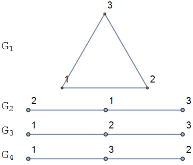
Figure 1: All labeled simply connected graphs of order 3.

By equations 14 through 17 we obtain:

$$\underline{W_{G_{1},G_{1}}} \rightarrow\begin{cases}\mathrm{vec}\left(X\right)=&\{x_{1},x_{2},x_{3},x_{4},x_{5},x_{1}+x_{2}+x_{3}-x_{4}-x_{5},\\ &x_{2}+x_{3}-x_{4},x_{1}+x_{3}-x_{5},-x_{3}+x_{4}+x_{5}\}\\ \mbox{null basis:}&\{1,0,0,0,0,1,0,1,0\}\\ &\{0,1,0,0,0,1,1,0,0\}\\ &\{0,0,1,0,0,1,1,1,-1\}\\ &\{0,0,0,1,0,-1,-1,0,1\}\\ &\{0,0,0,0,1,-1,0,-1,1\}\end{cases}$$ (18a)

$$\underline{W_{G_{2},G_{2}},W_{G_{2},G_{1}}} \rightarrow\begin{cases}\mathrm{vec}\left(X\right)=&\{x_{1},x_{2},x_{2},x_{2},x_{3},x_{1}+x_{2}-x_{3},x_{2},\\ &x_{1}+x_{2}-x_{3},x_{3}\}\\ \mbox{null basis:}&\{1,0,0,0,0,1,0,1,0\}\\ &\{0,1,1,1,0,1,1,1,0\}\\ &\{0,0,0,0,1,-1,0,-1,1\}\end{cases}$$ (18b)

$$\underline{W_{G_{3},G_{3}},W_{G_{3},G_{1}}} \rightarrow\begin{cases}\mathrm{vec}\left(X\right)=&\{x_{1},x_{2},x_{3},x_{2},x_{1}-x_{2}+x_{3},x_{2},x_{3},x_{2},x_{1}\}\\ \mbox{null basis:}&\{1,0,0,0,1,0,0,0,1\}\\ &\{0,1,0,1,-1,1,0,1,0\}\\ &\{0,0,1,0,1,0,1,0,0\}\end{cases}$$ (18c)

$$\underline{W_{G_{4},G_{4}},W_{G_{4},G_{1}}} \rightarrow\begin{cases}\mathrm{vec}\left(X\right)=&\{x_{1},x_{2},x_{3},x_{2},x_{1},x_{3},x_{3},x_{3},x_{1}+x_{2}-x_{3}\}\\ \mbox{null basis:}&\{1,0,0,0,1,0,0,0,1\}\\ &\{0,1,0,1,0,0,0,0,1\}\\ &\{0,0,1,0,0,1,1,1,-1\}\end{cases}$$ (18d)

$$\begin{array}[]{l}\underline{W_{G_{2},G_{3}},W_{G_{2},G_{4}},}\\ \underline{W_{G_{3},G_{4}}}\end{array} \rightarrow\begin{cases}\mathrm{vec}\left(X\right)=&\{x_{1},x_{1},x_{1},x_{1},x_{1},x_{1},x_{1},x_{1},x_{1}\}\\ \mbox{null basis:}&\{1,1,1,1,1,1,1,1,1\}\end{cases}$$ (18g)

We find the null spaces of the operators $W_{G_{2},G_{3}},W_{G_{2},G_{4}},$ and $W_{G_{3},G_{4}}$ in equation 18g according to equation 15

$$\mathrm{null}\left(W_{G_{2},G_{2}}\right)\cap\mathrm{null}\left(W_{G_{3},G_{3}}\right)=\mathrm{null}\left(W_{G_{2},G_{2}}\right)\cap\mathrm{null}\left(W_{G_{4},G_{4}}\right)$$ (19)

$$=\mathrm{null}\left(W_{G_{3},G_{3}}\right)\cap\mathrm{null}\left(W_{G_{4},G_{4}}\right)$$

$$=\{\{0,1,1,1,0,1,1,1,0\},\{1,0,0,0,1,0,0,0,1\}\},$$

from which we determine

$$\mathrm{null}\left(W_{G_{2},G_{3}}\right)=\mathrm{null}\left(W_{G_{2},G_{4}}\right)=\mathrm{null}\left(W_{G_{3},G_{4}}\right)$$ (20)

$$=\{1,1,1,1,1,1,1,1,1\}$$

by inspection.

These results and their interrelationships can be represented as an Euler diagram in which closed curves and intersecting zones represent a null space $\mathrm{null}\left(W_{G_{i},G_{j}}\right)$. As a mater of convenience, our Euler diagrams are non-area-proportional and wellformed up to labeling, sometimes having non-unique labeled curves [6] (see Fig. 2).

3.2 $\mathrm{null}\left(W_{G_{i},G_{j}}\right)$ for graphs of order 4

There are 38 different labeled simply connected graphs with order 4. When $i=j$, the null space of each $W_{G_{i},G_{i}}$ compose 32 distinct subspaces with double degeneracy among the 12 labeled path graphs (see Fig. 3). An Euler diagram illustrating the interrelationships of the subspaces enumerated in Fig. 3 is depicted in Fig. 4.

There are an additional ${38\choose 2}=703$ possible $W_{G_{i},G_{j}}$, where $i\neq j$, giving a total of 741 cases. All 741 possible $\mathrm{null}\left(W_{G_{i},G_{j}}\right)$ comprise a total of 50 distinct null spaces. A summary of the cardinality and degeneracy for each null space is given in Table 1.

4 Conclusion

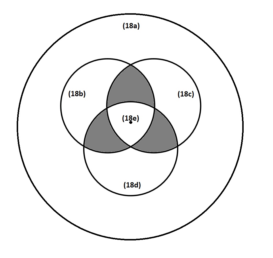
Figure 2: Euler diagram of all $\mathrm{null}\left(W_{G_{i},G_{j}}\right)$ for simply connected graphs of order 3. Each subspace/zone is annotated by the applicable equation number above. The shaded zones are empty.

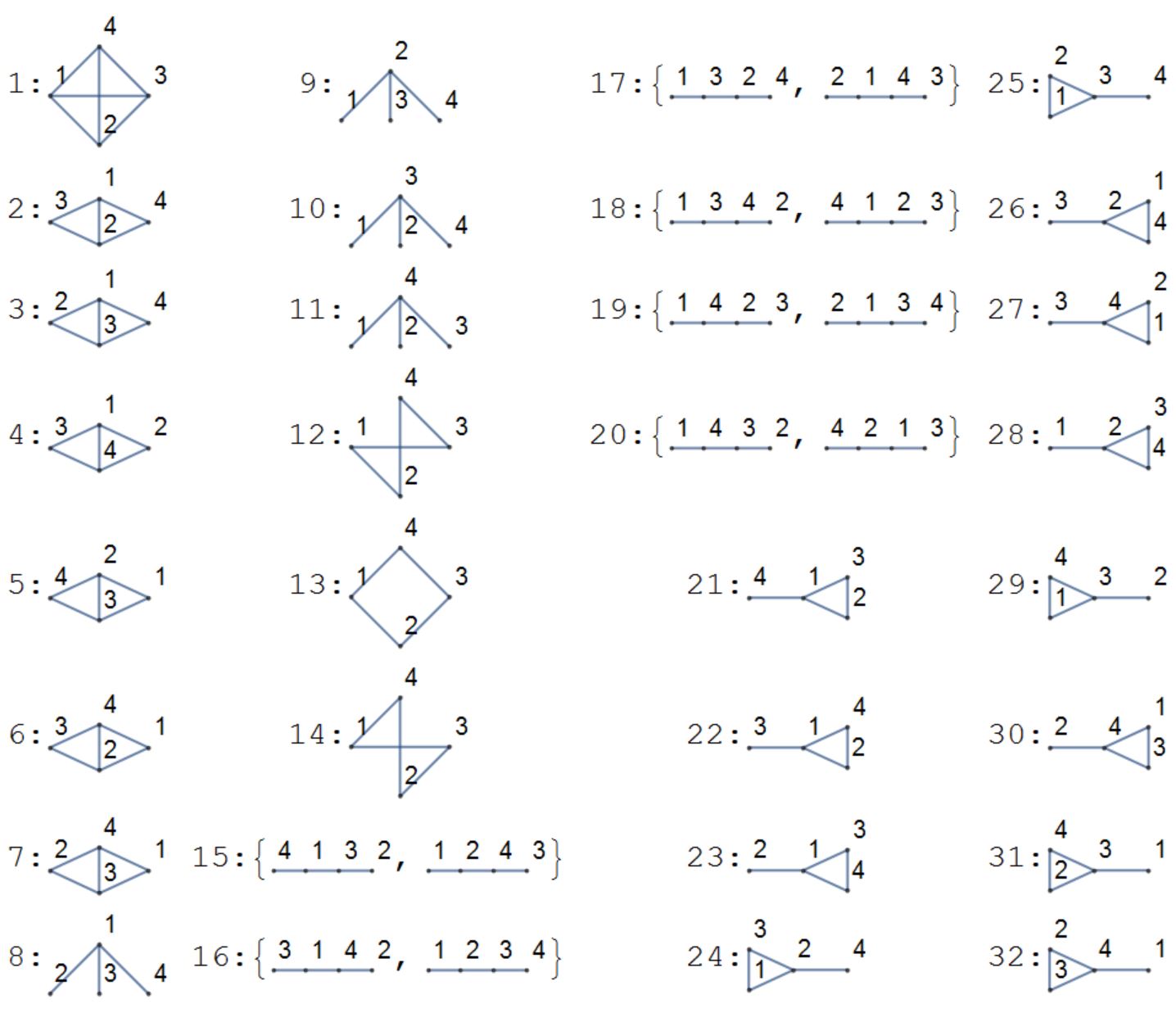
Figure 3: There are 38 labeled simply connected graphs $G_{i}$ of order 4. Each $\mathrm{null}\left(W_{G_{i},G_{i}}\right)$ compose 32 distinct subspaces with double degeneracy in the path graphs.

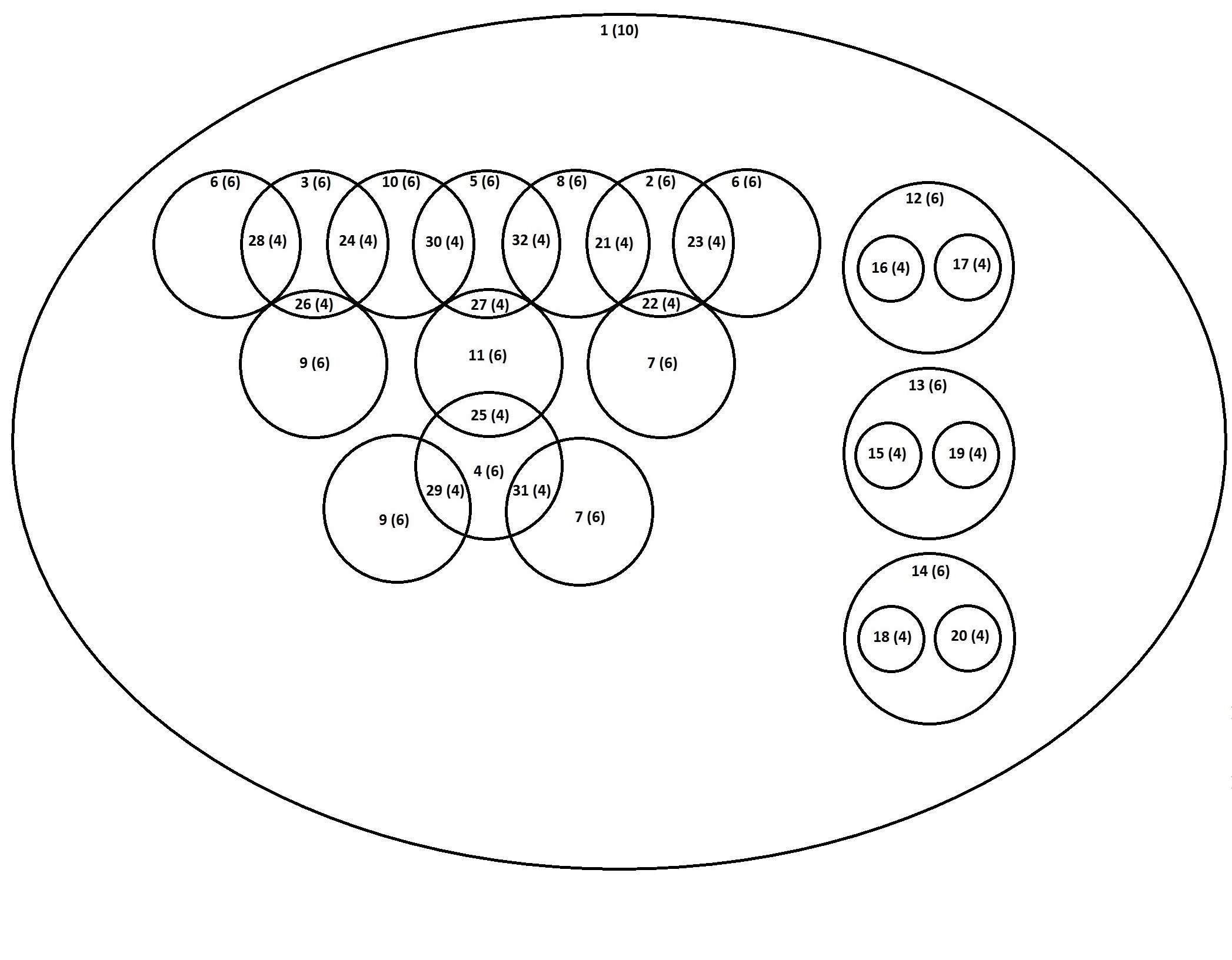
Figure 4: Euler diagram for the 32 enumerated null spaces of $W_{G_{i},G_{i}}$ in figure 3. The number of basis vectors spanning each null space is given in parentheses. (Only those intersections which are among the 32 distinct subspaces are shown.) Some labeled curves are not unique.

Zone	Degeneracy	Cardinality
1	1	10
2	2	6
3	2	6
4	2	6
5	2	6
6	2	6
7	2	6
8	2	6
9	2	6
10	2	6
11	2	6
12	2	6
13	2	6
14	2	6
15	7	4
16	7	4
17	7	4
18	7	4
19	7	4
20	7	4
21	5	4
22	5	4
23	5	4
24	5	4
25	5	4

Zone	Degeneracy	Cardinality
26	5	4
27	5	4
28	5	4
29	5	4
30	5	4
31	5	4
32	5	4
33	3	4
34	3	4
35	3	4
36	3	4
37	24	2
38	24	2
39	24	2
40	12	2
41	12	2
42	12	2
43	12	2
44	12	2
45	12	2
46	12	2
47	12	2
48	12	2
49	12	2
50	408	1

Table 1: The cardinality and degeneracy of the 50 distinct null spaces of $W_{G_{i},G_{j}}$ for all 38 labeled graphs of order 4.

References

References

- [1] E. Farhi and S. Gutmann. Quantum computation and decision trees. Phys. Rev. A, 58:915–928, 1998.
- [2] H. Gerhardt and J. Watrous. Continuous-time quantum walks on the symmetric group. In S. Arora, K. Jansen, J. Rolim, and A. Sahai, editors, Approximation, Randomization, and Combinatorial Optimization.. Algorithms and Techniques, volume 2764 of Lecture Notes in Computer Science, pages 290–301. Springer Berlin Heidelberg, 2003.
- [3] V. Vedral, M.B. Plenio, M.A. Rippin, and P.L. Knight. Quantifying entanglement. Phys. Rev. Lett, 78:2275–2278, 1997.
- [4] V. Simoncini. Computational methods for linear matrix equations. http://www.dm.unibo.it/~simoncin/matrixeq.pdf, March 2013. Survey article, Dept. of Mathematics, University of Bologna.
- [5] N. Higham. Sylvester’s influence on applied mathematics. http://www.manchester.ac.uk/mims/eprints, August 2014. Manchester Institute for Mathematical Sciences, The University of Manchester.
- [6] G. Stapleton, L. Zhang, J. Howse, and P. Rodgers. Drawing euler diagrams with circles. In A.K. Goel, M. Jamnik, and N.H. Narayanan, editors, 6th International Conference on the Theory and Application of Diagrams, pages 23–38. Springer-Verlag Berlin/Heidelberg, 2010.