Adiabatic Interactions of Manakov Solitons – Effects of Cross-modulation

Abstract

We investigate the asymptotic behavior of the Manakov soliton trains perturbed by cross-modulation in the adiabatic approximation. The multisoliton interactions in the adiabatic approximation are modeled by a generalized Complex Toda chain (GCTC). The cross-modulation requires special treating for the evolution of the polarization vectors of the solitons. The numerical predictions of the Manakov system are compared with the perturbed GCTC. For certain set of initial parameters GCTC describes very well the long-time evolution of the Manakov soliton trains.

1 Introduction

The Manakov model (MM) [28]

$$i\frac{\partial\vec{u}}{\partial t}+\frac{1}{2}\frac{\partial^{2}\vec{u}}{\partial x^{2}}+\langle\vec{u}{\;}^{\dagger},\vec{u}\rangle\vec{u}(x,t)=0,$$ (1)

where $\vec{u}(x,t)=(u_{1}(x,t),u_{2}(x,t))^{T}$, $t$ – time, $x$ – spatial coordinate, $\vec{u}^{\dagger}=(u_{1}^{*},u_{2}^{*})^{T}$ – hermitian conjugate to $\vec{u}$, $\langle\vec{u}^{\dagger},\vec{u}\rangle$ – scalar product of $\vec{u}^{\dagger}$ and $\vec{u}$, is the first generalization of the famous nonlinear Schrödinger equation [41] to multi-components. It finds a number of applications to physics: in nonlinear optics [3, 26, 28, 39], in Bose-Einstein condensates (BEC) [20, 21, 25, 31, 32, 33], in plasma physics and others [18, 30]). We specially mention some of them [3, 27, 32], which are closer to the types of interactions we consider.

Therefore it is an important problem to study the soliton interaction of (1) in the adiabatic approximation for multicomponent nonlinear Schrödinger equations. This task has been started some time ago in [5], [6]–[17], [23, 27, 34]. First, it was proved that a generalized version of the complex Toda chain (CTC) [5, 12, 14] describes rather well the $N$-soliton train behavior for wide set of soliton parameters. Since this generalized CTC is also integrable it allows one also to predict the asymptotic behavior of the $N$-soliton train for $t\to\infty$. The numerical tests comparing the trajectories of the solitons obtained as numerical solution of (1) with the trajectories predicted by the CTC showed an excellent agreement for up to 9-soliton trains.

The perturbed MM also finds a number of applications. For example, the equation

$$i\frac{\partial\vec{u}}{\partial t}+\frac{1}{2}\frac{\partial^{2}\vec{u}}{\partial x^{2}}+\langle\vec{u}{\;}^{\dagger},\vec{u}\rangle\vec{u}(x,t)=V(x)\vec{u}(x,t),$$ (2)

where $V(x)$ is an external potential can be viewed as one-dimensional model of the Gross-Pitaevski equations.Therefore it could be used to model quasi-one-dimensional BEC [25, 31, 33]. The system (2) is not integrable. However a perturbed GCTC was derived for several special types of potentials [6, 12, 14, 15].

Next we consider MM with cross-modulation parameter $\alpha_{2}$

$$\begin{split}i\frac{\partial u_{1}}{\partial t}+\frac{1}{2}\frac{\partial^{2}u_{1}}{\partial x^{2}}+\left[(1-\alpha_{2})|u_{1}|^{2}+(1+\alpha_{2})|u_{2}|^{2}\right]u_{1}(x,t)=0,\\ i\frac{\partial u_{2}}{\partial t}+\frac{1}{2}\frac{\partial^{2}u_{2}}{\partial x^{2}}+\left[(1+\alpha_{2})|u_{1}|^{2}+(1-\alpha_{2})|u_{2}|^{2}\right]u_{2}(x,t)=0,\end{split}$$ (3)

Obviously for small $\alpha_{2}$ the above equation can be still considered as a perturbed nonlinear vector Schrödinger equation. Eq. (3), as other perturbed versions of MM is also non-integrable [40]. Nevertheless for small $\alpha_{2}$ the adiabaticity is still possible and a respective generalized CTC model can be built. This is the main goal of the investigation in this paper. The model, Eq. (3) has been analyzed in detail previously by numerical methods in [4, 36, 37, 38] for wide range of $\alpha_{2}$.

In Sections 2 and 3 we introduce some preliminary facts and notations and apply the variational approach to the system (3) to derive a perturbed GCTC model that models the $N$-soliton trains in the presence of cross-modulation [7, 8] . The main difficulty here is to derive an adequate equation for the evolution of the polarization vectors $\vec{n}_{k}$. In Section 4 we briefly discuss how the GCTC can be used to investigate the asymptotic regimes of the soliton trains. In Section 5 we demonstrate that for some sets of soliton parameters the perturbed GCTC gives very good description for the cross-modulated MM. To this end we solve the cross-modulated MM numerically by using an implicit scheme of Crank-Nicolson type in complex arithmetic for the linear part of the operator and internal iterations for the nonlinear one. The concept of the internal iterations is applied (see [4]) in order to ensure the implementation of the conservation laws on difference level within the round-off error of the calculations [36, 37, 38]. The solutions of the relevant GCTC have been obtained using Maple. Knowing the numeric solution $\vec{u}$ of the perturbed MM we calculate he maxima of $(\vec{u}\,^{\dagger},\vec{u})$, compare them with the (numeric solutions) for $\xi_{k}(t)$ of the GCTC and plot the predicted by both models trajectories for each of the solitons. Thus we are able to analyze the effects of the cross-modulation on the soliton interactions. We end with some conclusions and discussions.

2 Posing the Problem. Adiabatic Approximation

Here we briefly remind the derivation of the CTC as a model describing the $N$-soliton interactions of multicomponent NLS systems using the variational approach [1, 2].

The main idea of the adiabatic approximation to soliton interactions is as follows [23]. Consider the MM, or one of its perturbed versions and analyze the dynamics of its solution with initial condition:

$$\begin{split}&\vec{u}(x,t=0)=\sum_{k=1}^{N}\vec{u}_{k}(x,t=0),\\ \vec{u}_{k}(x,t)&=u_{k}(x,t)\vec{n}_{k},\qquad u_{k}(x,t)={2\nu_{k}{\rm e}^{i\phi_{k}}\over\cosh(z_{k})}\end{split}$$ (4)

where

$$z_{k} =2\nu_{k}(x-\xi_{k}(t)), \qquad\xi_{k}(t) =2\mu_{k}t+\xi_{k,0},$$ (5)

$$\phi_{k} ={\mu_{k}\over\nu_{k}}z_{k}+\delta_{k}(t), \qquad\delta_{k}(t) =2(\mu_{k}^{2}+\nu_{k}^{2})t+\delta_{k,0}.$$

The $2$-component polarization vector is parametrized by

$$\begin{split}\vec{n}_{k}=\left(\cos(\theta_{k})e^{i\beta_{k}},\sin(\theta_{k})e^{-i\beta_{k}}\right)^{T}.\end{split}$$ (6)

It is obviously normalized by the conditions $(\vec{n}{\,}^{\dagger}_{k},\vec{n}_{k})=1$. The adiabatic approximation holds true if the soliton parameters satisfy [23]:

$$|\nu_{k}-\nu_{0}|\ll\nu_{0},\qquad|\mu_{k}-\mu_{0}|\ll\mu_{0},\qquad|\nu_{k}-\nu_{0}||\xi_{k+1,0}-\xi_{k,0}|\gg 1,$$ (7)

for all $k$, where $\nu_{0}={1\over N}\sum_{k=1}^{N}\nu_{k}$, and $\mu_{0}={1\over N}\sum_{k=1}^{N}\mu_{k}$ are the average amplitude and velocity, respectively. In fact we have two different scales:

$$\begin{split}|\nu_{k}-\nu_{0}|\simeq\varepsilon_{0}^{1/2},\qquad|\mu_{k}-\mu_{0}|\simeq\varepsilon_{0}^{1/2},\qquad|\xi_{k+1,0}-\xi_{k,0}|\simeq\varepsilon_{0}^{-1}.\end{split}$$ (8)

Next the basic idea of the adiabatic approximation is to derive a dynamical system for the soliton parameters which would describe their interaction. The initial condition (4) is not an exact $N$-soliton solution evaluated at $t=0$. It involves some small ($\simeq 1\%$) contribution of radiation due to the continuous spectrum. Adiabaticity also means that the solitons never overlap strongly. If this happens the approximation breaks down.

Initially this idea was proposed by Karpman and Solov’ev [23]. They inserted the initial condition in the NLS and after tedious calculations derived the dynamical system for the 8 parameters of the two solitons. A slightly different approach was proposed in [24, 22]. There the authors multiply the NLS eq. by a set of orthogonal functions and integrate. Such approach requires that the set orthogonal functions is convenient and complete.

An alternative derivation known as the variational approach was proposed by Anderson and Lisak [1, 2], see also [27]. Later this idea was generalized to $N$-soliton interactions [16, 11, 10, 17] and the corresponding dynamical system for the $4N$-soliton parameters was identified as a $N$-site CTC. The fact that the CTC, (just like its real counterpart – the Toda chain (RTC)) is completely integrable gives additional possibilities. A detailed comparative analysis between the solutions of the RTC and CTC [9] shows that the CTC allows for a variety of asymptotic regimes, see Section 4 below. More precisely, knowing the initial soliton parameters one can effectively predict the asymptotic regime of the soliton train. Another possible use of the same fact is, that one can describe the sets of soliton parameters responsible for each of the asymptotic regimes. Another important advantage of the adiabatic approach is, that one may consider the effects of various perturbations on the soliton interactions [23, 16].

These results were extended to treat the soliton interactions of the Manakov solitons. We derive a generalized version of the CTC as a model describing the behavior of the $N$-soliton trains of the MM [5, 7, 8, 12, 15]. This generalized CTC includes also the evolution of the polarization vectors $\vec{n}_{k}$. Using it one can predict the asymptotic regimes of the Manakov solitons and can describe the sets of soliton parameters that are responsible for each of the asymptotic regimes. Of course, just like for the scalar case, one can also analyze the effects of the various perturbations on the soliton interactions.

3 Derivation of the CTC as a model for the soliton interaction of the cross-modulated MM systems

We start with the Lagrangian of the cross-modulated MM systems:

$$\mathcal{L}=\int_{-\infty}^{\infty}dt\;{i\over 2}\left[\langle\vec{u}_{t}^{\dagger},\vec{u}\rangle-\langle\vec{u}\,^{\dagger},\vec{u}_{t}\rangle\right]-H.$$ (9)

where the Hamiltonian for the cross-modulated MM is

$$\begin{split}H=\int_{-\infty}^{\infty}dx\;\left(\frac{1}{2}\langle\vec{u}_{x}^{\dagger},\vec{u}_{x}\rangle-\frac{1}{2}(|u_{1}|^{2}+|u_{2}|^{2})^{2}+\frac{\alpha_{2}}{2}(|u_{1}|^{2}-|u_{2}|^{2})^{2}\right)\end{split}$$ (10)

It is easy to check that the Lagrangian equations of motion

$$\begin{split}\frac{\partial}{\partial t}\frac{\delta\mathcal{L}}{\delta u_{k,t}^{*}}-\frac{\delta\mathcal{L}}{\delta u_{k}^{*}}=0,\qquad k=1,2\end{split}$$ (11)

coincide with the equations (3).

The idea of the variational approach of [1, 2] is to insert the anzatz (4) into the Lagrangian, perform the integration over $x$ and retain only terms of the orders of $\varepsilon_{0}^{1/2}$ and $\varepsilon_{0}$. The first obvious observation is that only the nearest neighbors solitons will contribute such terms and

$$\mathcal{L}_{\rm eff}=\sum_{k=1}^{N}\mathcal{L}_{k}+\sum_{k=1}^{N}\sum_{n=k\pm 1}\widetilde{\mathcal{L}}_{kn}.$$ (12)

The leading order terms are the ones in $\mathcal{L}_{k}$ which correspond to the terms involving only the $k$-th soliton (see [8]):

$$\begin{split}\mathcal{L}_{k}&=4\nu_{k}\left({i\over 2}\left(\langle\vec{n}_{k}^{\dagger},\vec{n}_{k,t}\rangle-\langle\vec{n}_{k,t}^{\dagger},\vec{n}_{k}\rangle\right)+2\mu_{k}{d\xi_{k}\over dt}-{d\delta_{k}\over dt}-2\mu_{k}^{2}+{2\nu_{k}^{2}\over 3}\right)-\frac{4\alpha_{2}\nu_{k}}{3}\left(|n_{1,k}|^{2}-|n_{2,k}|^{2}\right)^{2}.\end{split}$$ (13)

Note that the terms that do not contain $t$-derivatives are of the order of 1. The order of the terms that contain $t$-derivatives can be established after one derives the evolution equations.

The second type of terms are the ones that involve only two different solitons, say $k$ and $p$. For example, consider

$$\begin{split}\mathcal{I}_{kp}&=\int_{-\infty}^{\infty}dx\;\left(u_{k}(x,t)u_{p}^{*}(x,t)+u_{k}^{*}(x,t)u_{p}(x,t)\right)\simeq 4\nu_{k}\nu_{p}\int_{-\infty}^{\infty}\frac{dz_{k}\;4\nu_{0}\cos(\phi_{k}-\phi_{p})}{\cosh(z_{k})\cosh(z_{p})}\\ &\simeq 4\nu_{0}\cos(\delta_{k}-\delta_{p})\Delta_{k,p}e^{-|\Delta_{k,p}|},\qquad\Delta_{k,p}=\xi_{k}-\xi_{p}.\end{split}$$ (14)

For $p=k\pm 1$ the right hand side of eq. (14) is the largest and is of the order of $\varepsilon$:

$$\begin{split}\varepsilon&\simeq\int_{-\infty}^{\infty}dx\;|u_{k}(x,t)u_{k+1}(x,t)|\simeq 2\Delta e^{-|\Delta|},\qquad\Delta\equiv\Delta_{k,k\pm 1}.\end{split}$$ (15)

In estimating the integral in (14) and (15) we also did several approximations: a) we replaced $\nu_{k}$ and $\nu_{k+1}$ by $\nu_{0}=1/N\sum_{k=1}^{N}\nu_{k}$ thus neglecting terms of the order of $\varepsilon^{3/2}$; b) we replaced $\sinh^{-1}(\Delta)$ by $2s_{k,k+1}e^{-\Delta}$ thus neglecting terms of the order of $\varepsilon^{2}$.

Comparing eqs. (14) and (15) we find that $\mathcal{I}_{kp}\simeq\varepsilon^{|k-p|}$. This means that the adiabatic approximation takes into account only the nearest neighbor interactions (i.e. the ones with $p=k\pm 1$) and neglects the ones with $|k-p|\geq 2$.

The third types of terms contain the effect of interactions of three and more different solitons. It is easy to see that these integrals contribute terms of order $\varepsilon^{2}$ and $\varepsilon^{3}$ respectively and therefore they are also neglected.

Keeping only the terms up to the order of $\varepsilon$ we obtain:

$$\mathcal{L}_{kn} =16\nu_{0}^{3}e^{-\Delta_{kn}}(R_{kn}+R_{kn}^{*})+\mathcal{O}(\varepsilon^{3/2}), \qquad R_{kn} =s_{kn}e^{i(\widetilde{\delta}_{n}-\widetilde{\delta}_{k})}\langle\vec{n}_{k}^{\dagger},\vec{n}_{n}\rangle,$$ (16)

$$\widetilde{\delta}_{k} =\delta_{k}-2\mu_{0}\xi_{k}, \qquad\Delta_{kn} =2s_{kn}\nu_{0}(\xi_{k}-\xi_{n}),$$

where $n=k\pm 1$ and $s_{k,k+1}=1$ and $s_{k,k-1}=-1$.

The next step is to consider the effective Lagrangian $\mathcal{L}_{\rm eff}$ (12) as a Lagrangian of the dynamical system, describing the motion of the $N$-soliton train and providing the equations of motion for the $(2s+2)N$ ($6N$ for the Manakov case) soliton parameters.

Let us first consider the unperturbed case, i.e., $\alpha_{2}=0$. Thus we arrive at the following set of dynamical equations for the soliton parameters:

$${d\xi_{k}\over dt} =2\mu_{k}, \;{d\delta_{k}\over dt} =2\mu_{k}^{2}+2\nu_{k}^{2},$$ (17)

$${d\nu_{k}\over dt} =8\nu_{0}^{3}\sum_{n=k\pm 1}e^{-\Delta_{kn}}i(R_{kn}-R_{kn}^{*}), \;{d\mu_{k}\over dt} =-8\nu_{0}^{3}\sum_{n=k\pm 1}e^{-\Delta_{kn}}(R_{kn}+R_{kn}^{*}).$$

Let us briefly discuss the order of the terms in the right hand sides of eqs. (17). Since we have assumed that the average velocity of the soliton train is $\mu_{0}=0$ then from eq. (8) it follows that the r.h.side of the first equation is $\mu_{k}\simeq\mathcal{O}(\varepsilon^{1/2})$. The r.h.side of the second equation in (17) for $d\delta_{k}/dt$ is of the order of 1. However in the next equations in (17) there enter only the differences $\delta_{k}-\delta_{k\pm 1}$ whose derivative, taking into account eq. (8) is again $\mathcal{O}(\varepsilon^{1/2})$. The right hand sides of the other two equations in (17) are of the order of $\mathcal{O}(\varepsilon)$.

In addition we need also the evolution equations for the polarization vectors $\vec{n}_{k}$ which are:

$$\begin{split}i\frac{\partial\vec{n}_{k}}{\partial t}+8\nu_{0}^{2}\sum_{n=k\pm 1}e^{-\Delta_{k,n}}R_{kn}\vec{n}_{n}+C\vec{n}_{k}=0,\end{split}$$ (18)

where $C$ is a $k$-independent real constant.

Thus for the unperturbed case $\alpha_{2}=0$ we have proven that $\frac{\partial\vec{n}_{k}}{\partial t}=\mathcal{O}(\epsilon)$. Since the scalar products $\langle\vec{n}_{k}^{\dagger},\vec{n}_{n}\rangle$ appear in the right hand side of eq. (17) in the factors $e^{-\Delta_{kn}}R_{kn}$, that are itself of the order $\mathcal{O}(\epsilon)$ it is evident that we can neglect the evolution of $\vec{n}_{k}$ using the initial values of $\left.\langle\vec{n}_{k}^{\dagger},\vec{n}_{n}\rangle\right|_{t=0}$.

3.1 Evolution of polarization vectors $\vec{n}_{k}$ – effect of cross-modulation

The cross-modulation changes substantially the evolution of the polarization vectors $\vec{n}_{k}$. Indeed, inserting into Eq.(11) $\vec{n}_{k}^{\dagger}$ instead of $u_{k}^{*}$ and neglecting the terms of the order of $\mathcal{O}(\epsilon)$ we obtain the following evolution equations for $\vec{n}_{k}$:

$$i\frac{\partial n_{1k}}{\partial t} =\frac{2\alpha_{2}}{3}\left(|n_{1k}|^{2}-|n_{2k}|^{2}\right)n_{1k},$$ (19)

$$i\frac{\partial n_{2k}}{\partial t} =-\frac{2\alpha_{2}}{3}\left(|n_{1k}|^{2}-|n_{2k}|^{2}\right)n_{2k},,$$

Divide the first line in (19) by $n_{1k}$ and the second one by $n_{2k}$. The imaginary parts give immediately that

$$\begin{split}\frac{\partial|n_{1k}|}{\partial t}=0,\qquad\frac{\partial|n_{2k}|}{\partial t}=0.\end{split}$$ (20)

If we use the parametrization: (6) then Eq.(20) means that

$$\begin{split}\frac{\partial\theta_{k}}{\partial t}=0.\end{split}$$ (21)

The real parts give immediately that

$$\begin{split}\beta_{k}(t)=-\frac{2\alpha_{2}}{3}\cos(2\theta_{k})t+\mbox{const\;}.\end{split}$$ (22)

Let us now calculate the scalar product:

$$\begin{split}\langle\vec{n}_{k+1},\vec{n}_{k}\rangle=\cos(\beta_{k+1}-\beta_{k})\cos(\theta_{k+1}-\theta_{k})-i\sin(\beta_{k+1}-\beta_{k})\cos(\theta_{k+1}+\theta_{k}).\end{split}$$ (23)

Now we can calculate the module and the phase of the scalar product:

$$\begin{split}|\langle\vec{n}_{k+1},\vec{n}_{k}\rangle|^{2}&=\cos^{2}(\beta_{k+1}-\beta_{k})\cos^{2}(\theta_{k+1}-\theta_{k})+\sin^{2}(\beta_{k+1}-\beta_{k})\cos^{2}(\theta_{k+1}+\theta_{k}),\\ \arg\langle\vec{n}_{k+1},\vec{n}_{k}\rangle&=-\arctan\left(\tan(\beta_{k+1}-\beta_{k})\frac{\cos(\theta_{k+1}+\theta_{k})}{\cos(\theta_{k+1}-\theta_{k})}\right).\end{split}$$ (24)

Thus, from Eqs.(17) we get:

$${d(\mu_{k}+i\nu_{k})\over dt}=4\nu_{0}\left[\langle\vec{n}_{k},\vec{n}_{k-1}\rangle e^{q_{k}-q_{k-1}}-\langle\vec{n}_{k+1},\vec{n}_{k}\rangle e^{q_{k+1}-q_{k}}\right],$$ (25)

where

$$\begin{split}q_{k}&=-2\nu_{0}\xi_{k}+k\ln 4\nu_{0}^{2}-i(\delta_{k}+\delta_{0}+k\pi-2\mu_{0}\xi_{k}),\\ \nu_{0}&={1\over N}\sum_{s=1}^{N}\nu_{s},\qquad\mu_{0}={1\over N}\sum_{s=1}^{N}\mu_{s},\qquad\delta_{0}={1\over N}\sum_{s=1}^{N}\delta_{s}.\end{split}$$ (26)

Besides, from (17) and (26) there follows (see [16]):

$${dq_{k}\over dt}=-4\nu_{0}(\mu_{k}+i\nu_{k}).$$ (27)

and

$${d^{2}q_{k}\over dt^{2}}=16\nu_{0}^{2}\left[\langle\vec{n}_{k+1},\vec{n}_{k}\rangle e^{q_{k+1}-q_{k}}-\langle\vec{n}_{k},\vec{n}_{k-1}\rangle e^{q_{k}-q_{k-1}}\right],$$ (28)

which proves the statement in [5]. Eq.(28), combined with the system of equations for the polarization vectors (19) provides the proper generalization of the CTC for the cross-modulated MM. Note, that for $\alpha_{2}=0$ the scalar products $\langle\vec{n}_{k+1},\vec{n}_{k}\rangle$ are time-independent and as a result the GCTC (28) is integrable. For $\alpha_{2}\neq 0$ however, the scalar products $\langle\vec{n}_{k+1},\vec{n}_{k}\rangle$ depend explicitly on $t$ as shown above, which makes the GCTC non-integrable.

The equations for the polarization vectors are nonlinear. So the whole system of equations for $q_{k}$ and $\vec{n}_{k}$ seems to be rather complicated and non-integrable even for the unperturbed MM. However, all terms in the right hand sides of the evolution equations for $\vec{n}_{k}$ are of the order of $\epsilon$. This allows us to neglect the evolution of $\vec{n}_{k}$ and to approximate them with their initial values. As a result we obtain that the $N$-soliton interactions for the multicomponent MM in the adiabatic approximation are modeled by the CTC, see Section 3.

4 GCTC and the Asymptotic Regimes of $N$-soliton Trains

The fact that the $N$-soliton trains for the scalar nonlinear Schrödinger equation are modeled by an integrable model – GCTC allowed one to predict their asymptotic behavior. The method to do so was based on the exact integrability of the CTC [11] and on its Lax representation.

Here we shall show, that similar results hold true also for the CTC (17) modeling the soliton trains of the MM. Indeed, following Moser [29] we introduce the Lax pair

$$\dot{L}=[B,L],$$ (29)

where

$$\begin{split}L=\sum_{k=1}^{N}\left(b_{k}E_{kk}+a_{k}(E_{k,k+1}+E_{k-1,k})\right),\qquad B=\sum_{k=1}^{N}a_{k}\left((E_{k,k+1}-E_{k-1,k}\right).\end{split}$$ (30)

Here the matrices $(E_{kn})_{pq}=\delta_{kp}\delta_{nq}$, and $E_{kn}=0$ whenever one of the indices becomes 0 or $N+1$; the other notations in (29) are as follows:

$$a_{k}={1\over 2}\sqrt{\langle\vec{n}_{k+1},\vec{n}_{k}\rangle}e^{(q_{k+1}-q_{k})/2},\qquad b_{k}={1\over 2}\left(\mu_{k}+i\nu_{k}\right).$$ (31)

One can check that the compatibility condition eq. (29) with $L$ and $B$ as in (30) is equivalent to the unperturbed GCTC (17).

The first consequence of the Lax representation is that the CTC has $N$ complex-valued integrals of motion provided by the eigenvalues of $L$ which we denote by $\zeta_{k}=\kappa_{k}+i\eta_{k}$, $k=1,\dots,N$. Indeed the Lax equation means that the evolution of $L$ is isospectral, i.e., $d\zeta_{k}/dt=0$.

Another important consequence from the results of Moser [29] is that for the real Toda chain one can write down explicitly its solutions in terms of the scattering data, which consist of pair series $\{\zeta_{k},r_{k}\}_{k=1}^{N}$ where $r_{k}$ are the first components of the properly normalized eigenvectors of $L_{0}$ [29, 35]. For the real Toda chain both $\zeta_{k}=\kappa_{k}$ and $r_{k}$ are real; besides all $\zeta_{k}$ are different. Next, Moser calculated the asymptotics of these solutions for $t\to\pm\infty$ and showed that $\kappa_{k}$ determine the asymptotic velocities of the particles.

The formulae derived by Moser can easily be extended to the complex case [9]. The important difference is that all important ingredients such as eigenvalues $\zeta_{k}$ and first components of the eigenvectors of $L$ normalized to 1 now become complex-valued. In addition, the important asset of $L$ for the RTC, namely that all eigenvalues are real and different, is also lost. However the asymptotics of the solutions for $t\to\pm\infty$ can be calculated with the result:

$$q_{k}(t)=-2\nu_{0}\zeta_{k}t-B_{k}+{\cal O}(e^{-Dt}),$$ (32)

where $D$ in (32) is some real positive constant, which is estimated by the minimal difference between the asymptotic velocities. Equating the real parts in Eq. (32) we obtain:

$$\lim_{t\to\infty}(\xi_{k}+2\kappa_{k}t)=\mbox{const\;},$$ (33)

which means that the real parts $\kappa_{k}$ of the eigenvalues of $L$ determine the asymptotic velocities for the CTC. This fact can be used to classify the regimes of asymptotic behavior.

Let us also remind the important differences between RTC and CTC. The only possible asymptotic behavior in the RTC is the asymptotically free motion of the soliton. For CTC the variety is much more depending on the number of solitons in the trains we differ three asymptotic regimes: asymptotically free regime, bound state regime, and mixed asymptotic regimes (for details see, for example [14, 15]).

The perturbed CTC taking into account the effects of the cross-modulation to the best of our knowledge is not integrable and does not allow Lax representation. Therefore we are applying numeric methods to solve it.

5 Results and Discussion

In order to understand better the influence of the cross-modulation we will reduce our considerations to two-soliton trains. We start with the case of trivial cross-modulation, i.e., $\alpha_{2}=0$. In this case the equations (3) become MM. In this case the trajectories of the soliton centers predicted by CTC and finite-difference implementation of MM are in excellent agreement. (Figure 1). The asymptotical behavior is asymptotically free regime. The temporal behavior of the MM solution is plotted in a separate graph (Figure 2).

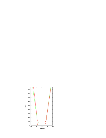
Figure 1: $\alpha_{2}=0$: $\delta_{1,2}=0,\pi$; $\nu_{1,2}=0.5$; $\xi_{1,2}=\pm 4$; $\mu_{1,2}=0$; $\beta_{1,2}=\pi/3,-\pi/4$; $\theta_{1}=\pi/4$, $\theta_{2}=\theta_{1}-\pi/20$. MM solution is plotted by solid line. CTC solution – by dashed line.

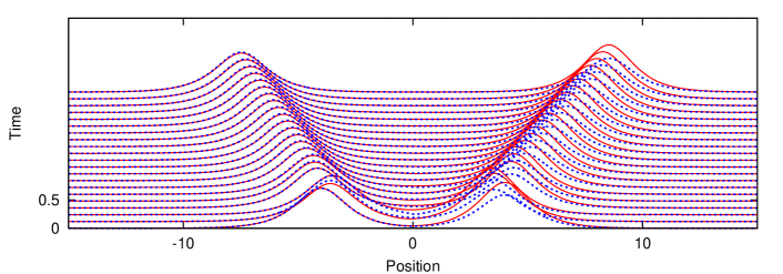
Figure 2: MM solution corresponding to data from Figure 1.

Having in mind the multiparametric manifold we fix the parameters in Figure 1 and vary only the cross-modulation. In Figure 3 the cross-modulation $\alpha_{2}=-0.045$ (left) and $\alpha_{2}=0.045$ (right), respectively. In both cases the asymptotic behavior is conserved though a phase shift of the trajectories of the soliton centers is observed.

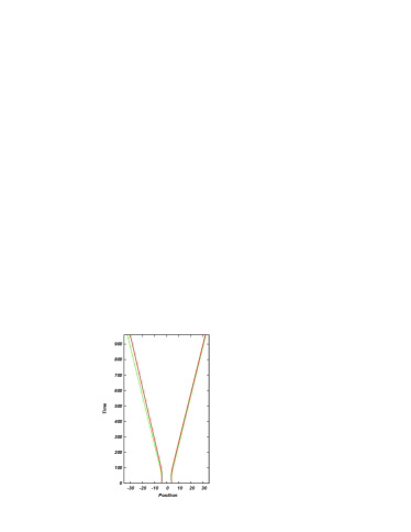
Figure 3: $\delta_{1,2}=0,\pi$; $\nu_{1,2}=0.5$; $\xi_{1,2}=\pm 4$; $\mu_{1,2}=0$; $\beta_{1,2}=\pi/3,-\pi/4$; $\theta_{1}=\pi/4$, $\theta_{2}=\theta_{1}-\pi/20$; $\alpha_{2}=-0.045$: (left); $\alpha_{2}=0.045$ (right). MM solution is plotted by solid line. CTC solution – by dashed line.

One more pair of computations with the same set of initial parameters are conducted, this time for $\alpha_{2}=\pm 0.06$. The results are plotted in Figures 4-left and 4-right and they are not differ qualitatively from those in Figures 3.

Figure 4: $\delta_{1,2}=0,\pi$; $\nu_{1,2}=0.5$; $\xi_{1,2}=\pm 4$; $\mu_{1,2}=0$; $\beta_{1,2}=\pi/3,-\pi/4$; $\theta_{1}=\pi/4$, $\theta_{2}=\theta_{1}-\pi/20$; $\alpha_{2}=-0.06$: (left); $\alpha_{2}=0.06$ (right). MM solution is plotted by solid line. CTC solution – by dashed line.

From the next pair of plots it is seen that the asymptotic prediction of CTC in presence of non-trivial cross-modulation can be improved if one varies the values of the initial phases $\delta_{1,2}$ (Figure 5-left) and polarization angles $\beta_{1,2}$ (Figure 5-right).

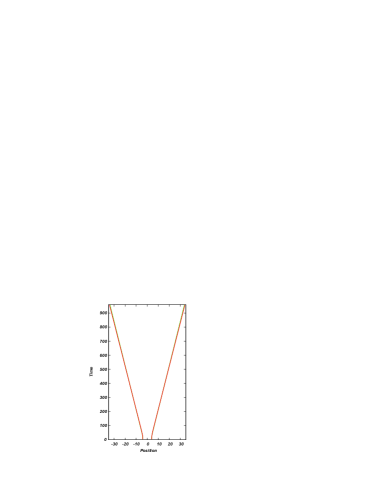
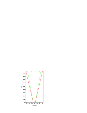
Figure 5: $\alpha_{2}=0.06$: $\delta_{1,2}=0$; $\nu_{1,2}=0.5$; $\xi_{1,2}=\pm 4$; $\mu_{1,2}=0$; $\beta_{1,2}=\pi/3,-\pi/4$; $\theta_{1,2}=\pi/4\pm\pi/20$ (left); $\delta_{1,2}=0,\pi$; $\nu_{1,2}=0.5$; $\xi_{1,2}=\pm 4$; $\mu_{1,2}=0$; $\beta_{1,2}=0$; $\theta_{1,2}=\pi/4\pm\pi/20$ (right). MM solution is plotted by solid line. CTC solution – by dashed line.

In all the considered cases angles $\theta_{1,2}$ are in the vicinity of $\pi/4$.

Next, the second our result is related to the linear temporal behavior of the polarization angles $\beta_{1,2}$. Concerning the last Figure 5-left GCTC gives slopes of the left soliton envelope $0.0123$ and for the right soliton envelope – $-0.024$. To make sure in the validity of these numerical predictions, Eq. (20), we evaluate the polarization angles from MM in another way, i.e.,

$$4\beta_{1,2}=\Im{\rm Log}\frac{u_{1}u_{2}^{*}}{u_{1}^{*}u_{2}}$$

where values of functions $u_{1}$ and $u_{2}$ correspond to the maxima of their envelopes, i.e., centers of the solitons. The latter formula comes right after equations (4) and (6). For the slopes we get $\pm 0.011$. The linear behavior of the polarization angles based on the above formula is well visible in Figure 6.

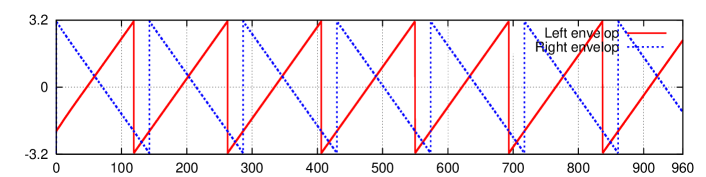
Figure 6: $\alpha_{2}=0.06$: Linear behavior of the polarization angles $\beta_{1,2}$ from Figure 5-left.

GCTC gives the same predictions for the slopes of the polarization angles of the solitons plotted in Figure 5-right, while MM predicts $\pm 0.127$. The linear behavior is presented in Figure 7.

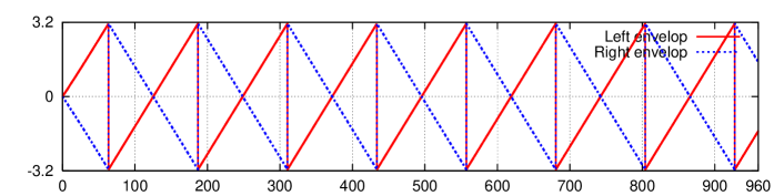
Figure 7: $\alpha_{2}=0.06$: Linear behavior of the polarization angles $\beta_{1,2}$ from Figure 5-right.

We consider and compare one more case, when $\alpha_{2}=-0.06$ (Figure 4-left). GCTC predicts zeroth slope of $\beta_{1}$ for the left soliton envelop and $0.021$ – for the right one. MM predicts $0.0002$ and $0.01$, respectively. The temporal behavior of $4\beta_{1,2}$ is given in Figure 8. The angles have been evaluated and plotted by module $2\pi$. These comparisons confirm cogently the GCTC prediction, Eq.(20), for the linear evolution of the polarization angles $\beta_{1,2}$.

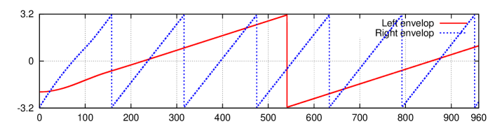
Figure 8: $\alpha_{2}=-0.06$: Linear behavior of the polarization angles $\beta_{1,2}$ from Figure 4-left.

Conclusions

It is well known that strong cross-modulation ( i.e. large $\alpha_{2}$) is not an adiabatic process. In fact it leads to creation of additional quasi-particles during the collisions, see Ref. [37].

That is why we studied the influence of weak cross-modulation (i.e. small $\alpha_{2}$) on the soliton trains of MM in the adiabatic approximation. We showed that for small values of $\alpha_{2}\simeq\sqrt{\epsilon}$ the adiabatic method still holds true. In particular, the GCTC model predicts that the angles $\beta_{k}$ parametrising the polarization vectors ((6)) depend linearly on time, which is confirmed by the numerical results, see Figures 5–7. The investigations elucidate the transition of the soliton solutions of the integrable Manakov model to the non-integrable nonlinear vector Schrödinger equation.

Appendix A Typical integrals

Here we list the typical integrals that appear in calculating the action for the cross-modulated MM. More details about their derivation and use to treat the effects of external potentials are given in [15] and the references therein.

We start with Fourier integrals of hyperbolic functions [19]:

$${\cal J}_{p}(a)=\int_{-\infty}^{\infty}{dz\,e^{iaz}\over 2\cosh^{p}z}=\int_{0}^{\infty}{dx\,\cos ax\over\cosh^{p}x},\qquad J_{p}(a)=\int_{-\infty}^{\infty}{dz\,e^{iaz}\sinh z\over 2\cosh^{p}z}.$$ (34)

They satisfy the recurrent relations:

$${\cal J}_{p}(a) ={a^{2}+(p-2)^{2}\over(p-1)(p-2)}{\cal J}_{p-2}(a), \qquad J_{p}(a) ={ia\over p-1}{\cal J}_{p-1}(a),$$ (35)

$${\cal J}_{1}(a) ={\pi\over 2\cosh{a\pi\over 2}}, \qquad{\cal J}_{2}(a) ={\pi a\over 2\sinh{a\pi\over 2}}.$$

Next we need more complicated integrals [19]:

$$\begin{split}K(a,\Delta)&\equiv\int_{-\infty}^{\infty}{dz\;e^{iaz}\over 2\cosh z\cosh(z+\Delta)}={\pi\over\sinh\Delta}{\sin(a\Delta/2)\over\sinh(\pi a/2)}e^{-ia\Delta/2}={\pi(1-e^{-ia\Delta})\over 2i\sinh(\Delta)\sinh(\pi a/2)},\\ L(a,\Delta)&\equiv\int_{-\infty}^{\infty}{dz\;e^{iaz}\sinh z\over 2\cosh^{2}z\cosh(z+\Delta)}={\pi i\over 2\sinh^{2}\Delta\sinh(\pi a/2)}\left[(1-e^{-ia\Delta})\cosh\Delta-ia\sinh\Delta\right],\end{split}$$ (36)

Of course, in our calculations we need only the terms of order $\varepsilon\simeq|\Delta|e^{-|\Delta|}$:

$$\begin{split}K(0,\Delta)&\equiv\int_{-\infty}^{\infty}{dz\over 2\cosh z\cosh(z+\Delta)}={\Delta\over\sinh\Delta},\\ L(0,\Delta)&\equiv\int_{-\infty}^{\infty}{dz\;\sinh z\over 2\cosh^{2}z\cosh(z+\Delta)}={1\over\sinh\Delta}\left[1-{\Delta\cosh\Delta\over\sinh\Delta}\right],\end{split}$$ (37)

which easily follow from the above expressions.

References

References

- [1] D. Anderson, and M. Lisak. Nonlinear asymmetric self-phase modulation and self-steepening of pulses in long optical waveguides Phys. Rev. A, 27:1393–1398, 1983.
- [2] D. Anderson, M. Lisak, and T. Reichel. Approximate analytical approaches to nonlinear pulse propagation in optical fibers: A comparison. Phys. Rev. A, 38: 1618–1620, 1988.
- [3] S. M. Baker, J. N. Elgin, and J. Gibbons. Polarization dynamics of solitons in birefringent fibers. Phys. Rev. E, 62:4325–4332, 1999.
- [4] C. I. Christov, S. Dost, and G. A. Maugin. Inelasticity of soliton collisions in systems of coupled NLS equations. Physica Scripta, 50:449–454, 1994.
- [5] V. S. Gerdjikov. -soliton interactions, the complex Toda chain and stability of NLS soliton trains. In: E. Kriezis (ed.), In Proc. of the Int. Symp. on Electromagnetic Theory, pages 307–309, Aristotle Univ. of Thessaloniki, vol. 1, 1998.
- [6] V. S. Gerdjikov. On soliton interactions of vector nonlinear Schrödinger equations., In M. D. Todorov and C. I. Christov (eds.), AMiTaNS’11, AIP CP1404, pages 57–67, AIP, Melville, NY, 2011.
- [7] V. S. Gerdjikov. Modeling soliton interactions of the perturbed vector nonlinear Schrödinger equation. Bulgarian J. Phys., 38:274–283, 2011.
- [8] V. S. Gerdjikov, E. V. Doktorov, and N. P. Matsuka. -soliton train and generalized complex Toda chain for Manakov system. Theor. Math. Phys., 151(3):762–773, 2007.
- [9] V. S. Gerdjikov, E. G. Evstatiev, and R. I. Ivanov. The complex Toda chains and the simple Lie algebras – solutions and large time asymptotics. J. Phys. A: Math & Gen., 31:8221–8232, 1998.
- [10] V. S. Gerdjikov, E. G. Evstatiev, D. J. Kaup, G. L. Diankov, and I. M. Uzunov. Stability and quasi-equidistant propagation of NLS soliton trains. Phys. Lett. A, 241:323–328, 1998.
- [11] V. S. Gerdjikov, D. J. Kaup, I. M. Uzunov, and E. G. Evstatiev. Asymptotic behavior of -soliton trains of the nonlinear Schrödinger equation. Phys. Rev. Lett., 77:3943–3946, 1996.
- [12] V. S. Gerdjikov, N. A. Kostov, E. V. Doktorov, and N. P. Matsuka. Generalized perturbed complex Toda chain for Manakov system and exact solutions of the Bose-Einstein mixtures. Mathematics and Computers in Simulation, 80:112–119, 2009.
- [13] V. S. Gerdjikov, N. A. Kostov, and T. I. Valchev. Solutions of multi-component NLS models and spinor Bose-Einstein condensates. Physica D, 238:1306–1310, 2009, ArXiv:0802.4398 [nlin.SI].
- [14] V. S. Gerdjikov and M. D. Todorov. -soliton interactions for the Manakov system. Effects of external potentials. In R. Carretero-Gonzalez et al. (eds.), Localized Excitations in Nonlinear Complex Systems, Nonlinear Systems and Complexity 7, pages 147–169, Springer International Publishing Switzerland, 2014, doi 10.1007/978-3-319-02057-07.
- [15] V. S. Gerdjikov and M. D. Todorov. ‘On the effects of sech-like potentials on Manakov solitons. In M. D. Todorov (ed.) AMiTaNS’13, AIP CP1561, pages 75–83, AIP, Melville, NY, 2013, doi 10.1063/1.4827216.
- [16] V. S. Gerdjikov, I. M. Uzunov, E. G. Evstatiev, and G. L. Diankov. Nonlinear Schrödinger equation and -soliton interactions: Generalized Karpman-Soloviev approach and the complex Toda chain. Phys. Rev. E, 55(5):6039–6060, 1997.
- [17] V. S. Gerdjikov and I. M. Uzunov. Adiabatic and non-adiabatic soliton interactions in nonlinear optics. Physica D, 152-153:355–362, 2001.
- [18] V. S. Gerdjikov, G. Vilasi, and A. B. Yanovski. Integrable Hamiltonian Hierarchies. Spectral and Geometric Methods. Lecture Notes in Physics vol. 748, Springer Verlag, Berlin-Heidelberg-New York, 2008, ISBN: 978-3-540-77054-1.
- [19] I. S. Gradshteyn, I. M. Ryzhik. Table of Integrals, Series, and Products. Corrected and enlarged edition. Academic Press, 2014.
- [20] T.-L. Ho. Spinor Bose condensates in optical traps. Phys. Rev. Lett., 81:742, 1998.
- [21] J. Ieda, T. Miyakawa, and M. Wadati. Exact analysis of soliton dynamics in spinor Bose-Einstein condensates. Phys. Rev Lett., 93:194102, 2004.
- [22] A. Janutka. Stability of multicomponent-soliton trains. Phys. Scr. 82:045001 (7pp), 2010, doi:10.1088/0031-8949/82/04/045001
- [23] V. I. Karpman and V. V. Solov’ev. A Perturbational approach to the two-solition systems. Physica D, 3:487–502, 1981.
- [24] Y. Lai and H.A. Haus. Quantum theory of self-induced transparency solitons: A linearization approach. Phys. Rev. A, 42:2925, 1990.
- [25] P. G. Kevrekidis, D. J. Frantzeskakis, and R. Carretero-Gonzalez (eds.). Emergent Nonlinear Phenomena in Bose-Einstein Condensates: Theory and Experiment. Springer, Vol. 45, 2008.
- [26] T. I. Lakoba and D. J. Kaup. Perturbation theory for the Manakov soliton and its applications to pulse propagation in randomly birefringent fibers. Phys. Rev. E, 56:6147–6165, 1997.
- [27] B. A. Malomed. Variational methods in nonlinear fiber optics and related fields. Progr. Opt., 43:71–193, 2002.
- [28] S. V. Manakov. On the theory of two-dimensional stationary self-focusing of electromagnetic waves. Zh. Eksp. Teor. Fiz., 65: 1392, 1973. English translation: Sov. Phys. JETP 38:248, 1974.
- [29] J. Moser. Dynamical Systems, Theory and Applications. Lecture Notes in Physics vol. 38, Springer Verlag, Berlin, 467 pages, 1975.
- [30] S. P. Novikov, S. V. Manakov, L. P. Pitaevski, and V. E. Zakharov. “Theory of Solitons, the Inverse Scattering Method,” Consultant Bureau, New York, 1984.
- [31] L. P. Pitaevskii and S. Stringari. “Bose-Einstein Condensation.” Oxford University Press, Oxford, UK, 2003.
- [32] T. Ohmi and K. Machida. Bose-Einstein condensation with internal degrees of freedom in alkali atom gases. J. Phys. Soc. Jpn., 67:1822, 1998.
- [33] V. M. Perez-Garcia, H. Michinel, J. I. Cirac, M. Lewenstein, and P. Zoller. Dynamics of Bose-Einstein condensates: Variational solutions of the Gross-Pitaevskii equations. Phys. Rev. A, 56:1424–1432, 1997.
- [34] V. S. Shchesnovich and E. V. Doktorov. Perturbation theory for solitons of the Manakov system. Phys. Rev. E, 55:7626, 1997.
- [35] M. Toda. “Theory of Nonlinear Lattices.”, Springer Verlag, Berlin, 1989.
- [36] M. D. Todorov and C. I. Christov. Conservative numerical scheme in complex arithmetic for coupled nonlinear Schrodinger equations. Discrete and Continuous Dynamical Systems, Supplement 2007, 982–992.
- [37] M. D. Todorov and C. I. Christov. Impact of the large cross-modulation parameter on the collision dynamics of quasi-particles governed by vector NLSE. Mathematics and Computers in Simulation, 80:46–55, 2008.
- [38] M. D. Todorov and C. I. Christov. Collision dynamics of elliptically polarized solitons in coupled nonlinear Schrödinger equations. Mathematics and Computers in Simulation, 82:1221–1232, 2012.
- [39] J. Yang. Suppression of Manakov soliton interference in optical fibers. Phys. Rev. E, 65:036606, 2002.
- [40] V.E. Zakharov and E.I. Schulman. To the integrability of the system of two coupled nonlinear Schrödinger equations. Physica 4D, 270-274, 1982.
- [41] V. E. Zakharov and A. B. Shabat. Exact theory of two-dimensional self-focusing and one-dimensional self-modulation of waves in nonlinear media. English translation: Soviet Physics-JETP, 34:62–69, 1972.