Improved Rademacher symmetrization through a Wasserstein based measure of asymmetry

Abstract

We propose of an improved version of the ubiquitous symmetrization inequality making use of the Wasserstein distance between a measure and its reflection in order to quantify the symmetry of the given measure. An empirical bound on this asymmetric correction term is derived through a bootstrap procedure and shown to give tighter results in practical settings than the original uncorrected inequality. Lastly, a wide range of applications are detailed including testing for data symmetry, constructing nonasymptotic high dimensional confidence sets, bounding the variance of an empirical process, and improving constants in Nemirovski style inequalities for Banach space valued random variables.

1 Introduction

The symmetrization inequality is a ubiquitous result in the probability in Banach spaces literature and in the concentration of measure literature. Dating back at least to Paul Lévy, it is found in the classic text of Ledoux and Talagrand (1991), Section 6.1, and the more recent Boucheron et al. (2013), Section 11.3. Giné and Zinn (1984) use symmetrization in the context of empirical process theory, which is followed by a collection of more recent appearances such as Panchenko (2003); Koltchinskii (2006); Giné and Nickl (2010); Arlot et al. (2010); Lounici and Nickl (2011); Kerkyacharian et al. (2012); Fan (2011).

The symmetrization inequality is as follows. Let $(B,\lVert\cdot\rVert)$ be a Banach space, and let $X_{1},\ldots,X_{n}\in B$ be independent and identically distributed random variables with measure $\mu$. Let $\varepsilon_{1},\ldots,\varepsilon_{n}$ be independent and identically distributed Rademacher random variables, which are such that $\mathrm{P}\left(\varepsilon_{i}=1\right)=\mathrm{P}\left(\varepsilon_{i}=-1\right)=1/2$. These are sometimes referred to as symmetric Bernoulli or random signs. The symmetrization inequality is

$$\mathrm{E}\left\lVert\frac{1}{n}\sum_{i=1}^{n}(X_{i}-\mathrm{E}X_{i})\right\rVert\leq 2\mathrm{E}\left\lVert\frac{1}{n}\sum_{i=1}^{n}\varepsilon_{i}(X_{i}-\mathrm{E}X_{i})\right\rVert.$$

This can be readily proved via Jensen’s Inequality and the insight that if $Z$ is a symmetric random variable, that is $Z\overset{\text{d}}{=}-Z$, then $Z\overset{\text{d}}{=}\varepsilon Z$.

The most notable oversight of this result is that it does not incorporate any measure of the symmetry of the data. Specifically, in the extreme case that the $X_{i}$ are symmetric about their mean, then the coefficient of 2 can be dropped and the inequality becomes an equality. Taking note of this fact, Arlot et al. (2010) state that “it can be shown that this factor of 2 is unavoidable in general for a fixed $n$ when the symmetry assumption is not satisfied, although it is unnecessary when $n$ goes to infinity.” They furthermore “conjecture that an inequality holds under an assumption less restrictive than symmetry (e.g., concerning an appropriate measure of skewness of the distribution ).” Hence, in response to this conjecture, we propose an improved symmetrization inequality making use of Wasserstein distance and Hilbert space geometry in order to account for the symmetry, or lack thereof, of the distribution of the $X_{i}$ under analysis. The main contribution of this paper is that for some Hilbert space $H$ and $X_{1},\ldots,X_{n}\in H$ iid random variables with measure $\mu$, there is for a fixed constant $C(\mu)$ depending only on the symmetry of the underlying measure $\mu$ of the $X_{i}$, which quantifies the symmetry of $\mu$, such that

$$\mathrm{E}\left\lVert\frac{1}{n}\sum_{i=1}^{n}(X_{i}-\mathrm{E}X_{i})\right\rVert\leq\mathrm{E}\left\lVert\frac{1}{n}\sum_{i=1}^{n}\varepsilon_{i}(X_{i}-\mathrm{E}X_{i})\right\rVert+\frac{C(\mu)}{n^{1/2}}.$$

This result is detailed and proved in Section 2.2. Furthermore, an empirical bound, $C_{n}(\mu)$, on the constant $C$ can be calculated as is done in Section 3. In the case that the distribution of the $X_{i}$ is symmetric, our data driven estimate $C_{n}(X)=O(n^{-1/2})$ implying an $n^{-1}$ rate of convergence to the desired zero for the additive term above. Applications of this result to testing the symmetry of a data set, constructing nonasymptotic high dimensional confidence sets, bounding the variance of an empirical process, and improving coefficients in probabilistic inequalities in the Banach space setting are given in Section 4.

2 Symmetrization

2.1 Definitions

We first require the standard notions of Wasserstein distance and Wasserstein space as stated below. For a thorough introduction to such topics, see Villani (2008).

Definition 2.1 (Wasserstein Distance).

Let $(\mathcal{X},d)$ be a Polish space and $p\in[1,\infty)$. For two probability measures $\mu$ and $\nu$ on $\mathcal{X}$, the Wasserstein $p$ distance is

$$W_{p}(\mu,\nu)=\inf_{\gamma\in\Pi(\mu,\nu)}\left(\int_{\mathcal{X}\times\mathcal{X}}d(x,y)^{p}d\gamma(x,y)\right)^{1/p}$$

where the infimum is taken over all measures $\gamma$ on $\mathcal{X}\times\mathcal{X}$ with marginals $\mu$ and $\nu$.

An equivalent and useful formulation of Wasserstein distance is

$$W_{p}(\mu,\nu)=\inf_{(X,Y)}\left(\mathrm{E}\,d(X,Y)^{p}\right)^{1/p}$$

where the infimum is taken over all possible joint distributions of $X$ and $Y$ with marginals $\mu$ and $\nu$, respectively.

Definition 2.2 (Wasserstein Space).

Let $P(\mathcal{X})$ be the space of probability measures on $\mathcal{X}$. The Wasserstein space is

$$P_{p}(\mathcal{X}):=\left\{\mu\in P(\mathcal{X})\,\middle|\,\int_{\mathcal{X}}d(x_{0},x)^{p}\mu(dx)<\infty\right\}$$

for any arbitrary choice of $x_{0}$. This is the space of measures with finite $p$th moment.

Convergence in Wasserstein space is characterized by weak convergence of measure and convergence in $p$th moment. From Theorem 6.8 of Villani (2008), convergence in Wasserstein distance is equivalent to weak convergence in $P_{p}(\mathcal{X})$. Hence, for a sequence of measures $\mu_{n}$,

$$W_{p}(\mu_{n},\mu)\rightarrow 0\text{ if and only if }\mu_{n}\xrightarrow{\text{d}}\mu\text{ and }\int_{\mathcal{X}}x^{p}d\mu_{n}(x)\rightarrow\int_{\mathcal{X}}x^{p}d\mu(x).$$

Secondly, we will make use of empirical measures and the already mentioned Rademacher random variables.

Definition 2.3 (Empirical Measure).

For independent and identically distributed random variables $X_{1},\ldots,X_{n}$, the empirical measure is a random measure defined as

$$\mu_{n}(A):=\frac{1}{n}\sum_{i=1}^{n}\bm{1}_{X_{i}\in A}$$

for some measurable set $A$. We will denote the empirical measure of the reflected variables $-X_{1},\ldots,-X_{n}$ by $\mu_{n}^{-}$.

Definition 2.4 (Rademacher Distribution).

A random variable $\varepsilon\in\mathbb{R}$ has a Rademacher distribution if $\mathrm{P}\left(\varepsilon=1\right)=\mathrm{P}\left(\varepsilon=-1\right)=1/2.$ In Section 3, we will also consider more general Rademacher$(p)$ distributions where $\mathrm{P}\left(\varepsilon=1\right)=p$ and conversely $\mathrm{P}\left(\varepsilon=-1\right)=1-p$.

2.2 Symmetrization Result

In the following lemma, we bound the expectation on the left by the sum of a “symmetric” term and an “asymmetric” term.

Lemma 2.5.

Let $H$ be an Hilbert space, and let $X_{1},\ldots,X_{n}\in H$ be independent and identically distributed random variables with common law $\mu$. Define $\mu^{-}$ to be the law of $-X$. Furthermore, let $\varepsilon_{1},\ldots,\varepsilon_{n}$ be independent and identically distributed Rademacher random variables also independent of the $X_{i}$. Then, for any 1-Lipschitz function $\psi$,

$$\mathrm{E}\psi\left(\sum_{i=1}^{n}(X_{i}-\mathrm{E}X_{i})\right)\leq\mathrm{E}\psi\left(\sum_{i=1}^{n}\varepsilon_{i}(X_{i}-\mathrm{E}X_{i})\right)+\sqrt{\frac{n}{2}}W_{2}(\mu,\mu^{-})$$

where $W_{2}$ is the Wasserstein 2 distance.

Proof.

For a Polish space $\mathcal{X}$, let $\Pi(\mu,\nu)$ be the space of all product measures on $\mathcal{X}\times\mathcal{X}$ with marginals $\mu$ and $\nu$. For $\delta\in(0,1)$, let $\Pi_{\delta}(\mu,\nu)$ be the space of all product measures with marginals $\mu$ and $\nu_{\delta}=\delta\mu+(1-\delta)\nu$. For $\gamma\in\Pi(\mu,\nu)$ and $\eta\in\Pi(\mu,\mu)$, the measure $\delta\eta+(1-\delta)\gamma\in\Pi_{\delta}(\mu,\nu)$. Hence,

$$W_{p}^{p}(\mu,\nu_{\delta}) =\inf_{\gamma_{\delta}\in\Pi(\mu,\nu_{\delta})}\int_{\mathcal{X}\times\mathcal{X}}d(x,y)^{p}d\gamma_{\delta}(x,y)$$

$$\leq\inf_{\eta\in\Pi(\mu,\mu),\,\gamma\in\Pi(\mu,\nu)}\int_{\mathcal{X}\times\mathcal{X}}d(x,y)^{p}d(\delta\eta+(1-\delta)\gamma)(x,y)$$

$$=\inf_{\gamma\in{\Pi}(\mu,\nu)}(1-\delta)\int_{\mathcal{X}\times\mathcal{X}}d(x,y)^{p}d\gamma(x,y)$$

$$=(1-\delta)W_{p}^{p}(\mu,\nu).$$

The inequality on the second lines above arises from taking the infimum over a more restrictive set. The law of $\varepsilon X$ is $\frac{1}{2}(\mu+\mu^{-})$. Hence, for our purposes, the above implies that

$$W_{2}\left(\mu,\frac{\mu+\mu^{-}}{2}\right)\leq\frac{1}{\sqrt{2}}W_{2}(\mu,\mu^{-}).$$

Define $\mu^{*n}$ to be the law of $\sum_{i=1}^{n}(X_{i}-\mathrm{E}X_{i})$ and $\tilde{\mu}^{*n}$ to be the law of $\sum_{i=1}^{n}\varepsilon_{i}(X_{i}-\mathrm{E}X_{i})$. Then,

$$~{}~{}~{}~{}\mathrm{E}\psi\left(\sum_{i=1}^{n}(X_{i}-\mathrm{E}X_{i})\right)-\mathrm{E}\psi\left(\sum_{i=1}^{n}\varepsilon_{i}(X_{i}-\mathrm{E}X_{i})\right)\leq$$

$$\leq\sup_{\lVert\phi\rVert_{Lip}\leq 1}\left\{\mathrm{E}\phi\left(\sum_{i=1}^{n}(X_{i}-\mathrm{E}X_{i})\right)-\mathrm{E}\phi\left(\sum_{i=1}^{n}\varepsilon_{i}(X_{i}-\mathrm{E}X_{i})\right)\right\}$$

$$\leq W_{1}\left(\mu^{*n},\tilde{\mu}^{*n}\right)$$

$$\leq W_{2}\left(\mu^{*n},\tilde{\mu}^{*n}\right)$$

$$\leq\sqrt{n}W_{2}\left(\mu,\frac{\mu+\mu}{2}^{-}\right)$$

$$\leq\sqrt{\frac{n}{2}}W_{2}(\mu,\mu^{-})$$

where the second, third, and fourth inequality come respectively from Lemmas A.1, A.2, and A.3 in the appendix. Rearranging the terms gives the desired result. ∎

This lemma leads immediately to the following theorem. The intuition behind this theorem is that averaging a collection of random variables has an inherent smoothing and symmetrizing effect. Thus, as the sample size $n$ increases, the difference between the expectations of the true average and the Rademacher average become negligible.

Theorem 2.6.

Using the setting of Lemma 2.5 with either of the following two conditions that

1. $\psi$ is additionally positive homogeneous (e.g. a norm), or

2. the metric $d$ is positive homogeneous in the sense that for $a\in\mathbb{R}$, $d(ax,ay)=\lvert a\rvert d(x,y)$,

then

$$\left\lvert\mathrm{E}\psi\left(\frac{1}{n}\sum_{i=1}^{n}(X_{i}-\mathrm{E}X_{i})\right)-\mathrm{E}\psi\left(\frac{1}{n}\sum_{i=1}^{n}\varepsilon_{i}(X_{i}-\mathrm{E}X_{i})\right)\right\rvert=O\left(\frac{1}{\sqrt{n}}\right).$$

Proof.

Running the proof of Lemma 2.5 after swapping $\sum_{i=1}^{n}(X_{i}-\mathrm{E}X_{i})$ and $\sum_{i=1}^{n}\varepsilon_{i}(X_{i}-\mathrm{E}X_{i})$ gives the lower deviation

$$\mathrm{E}\psi\left(\sum_{i=1}^{n}(X_{i}-\mathrm{E}X_{i})\right)\geq\mathrm{E}\psi\left(\sum_{i=1}^{n}\varepsilon_{i}(X_{i}-\mathrm{E}X_{i})\right)-\sqrt{\frac{n}{2}}W_{2}(\mu,\mu^{-}).$$

Under condition 1, the result is immediate.

Under condition 2, let $\mu$ be the law of $(X_{i}-\mathrm{E}X_{i})$ as before. Then, redefining $\mu^{*n}$ to be the law of $\sum_{i=1}^{n}\frac{1}{n}(X_{i}-\mathrm{E}X_{i})$ and $\tilde{\mu}^{*n}$ to be the law of $\sum_{i=1}^{n}\frac{1}{n}\varepsilon_{i}(X_{i}-\mathrm{E}X_{i})$ results in

$$W_{2}(\mu^{*n},\tilde{\mu}^{*n}) \leq\sqrt{n}\inf_{(X,Y)}\left(\mathrm{E}\,d(X/n,Y/n)^{2}\right)^{1/2}$$

$$=\frac{1}{\sqrt{2n}}W_{2}(\mu,\mu^{-})$$

where the infimum is taken over all joint distributions of $X$ and $Y$ with marginals $\mu$ and $\frac{\mu+\mu^{-}}{2}$, respectively. The desired result follows. ∎

3 Empirical estimate of $W_{2}(\mu,\mu^{-})$

In order to explicitly make use of the above results, an empirical estimate of $W_{2}(\mu,\mu^{-})$ is required. We first establish the following bound.

Proposition 3.1.

Let $X_{1},\ldots,X_{n}$ be iid with law $\mu$ and let $Y_{1},\ldots,Y_{n}$ be iid with law $\nu$. Furthermore, let $\mu_{n}$ and $\nu_{n}$ be the empirical distributions of $\mu$ and $\nu$, respectively. Then,

$$W_{p}^{p}(\mu,\nu)\leq\mathrm{E}W_{p}^{p}(\mu_{n},\nu_{n}).$$

Proof.

The following infima are taken over the joint distributions of the random variables in question. Let $X$ and $Y$ be random variables of law $\mu$ and $\nu$, respectively. Also, let $S_{n}$ be the group of permutations on $n$ elements.

$$W_{p}^{p}(\mu,\nu) =\inf_{(X,Y)}\mathrm{E}d(X,Y)^{p}$$

$$=\inf_{(X_{1},\ldots,X_{n},Y_{1},\ldots,Y_{n})}\mathrm{E}\left\{\frac{1}{n}\sum_{i=1}^{n}d(X_{i},Y_{i})^{p}\right\}$$

$$\leq\mathrm{E}\min_{\rho\in S_{n}}\left\{\frac{1}{n}\sum_{i=1}^{n}d(X_{i},Y_{\rho(i)})^{p}\right\}$$

$$=\mathrm{E}W_{p}^{p}(\mu_{n},\nu_{n})$$

where the above inequality arises by replacing the infimum over all possible joint distributions of the $X_{i}$ and $Y_{i}$ with a specific joint distribution. ∎

The following subsections establish that it is reasonable to replace $W_{2}(\mu,\mu^{-})$ with a data driven estimate of $\mathrm{E}W_{2}(\mu_{n},\mu_{n}^{-})$ in Lemma 2.5 and Theorem 2.6. Rates of convergence of $W_{2}(\mu_{n},\mu_{n}^{-})$ are presented, and a bootstrap estimator for $\mathrm{E}W_{2}(\mu_{n},\mu_{n}^{-})$ is proposed and tested numerically.

3.1 Rate of convergence of empirical estimate

As $W_{p}(\cdot,\cdot)$ is a metric, the triangle inequality implies that

$$W_{p}(\mu,\mu^{-}) \leq W_{p}(\mu,\mu_{n})+W_{p}(\mu_{n},\mu_{n}^{-})+W_{p}(\mu_{n}^{-},\mu^{-})$$

$$\leq 2W_{p}(\mu,\mu_{n})+W_{p}(\mu_{n},\mu_{n}^{-}),$$

and therefore,

$$\lvert W_{p}(\mu,\mu^{-})-W_{p}(\mu_{n},\mu_{n}^{-})\rvert\leq 2W_{p}(\mu,\mu_{n}).$$

By Lemma A.4, $W_{p}(\mu,\mu_{n})\rightarrow 0$ with probability one making the discrepancy negligible for large data sets. However, it is also possible to get a hard upper bound on this term; specifically, the recent work of Fournier and Guillin (2015) proposes explicit moment bounds on $W_{p}(\mu,\mu_{n})$. Their result can be used to demonstrate the speed with which our empirical measure of asymmetry, $W_{2}(\mu_{n},\mu_{n}^{-})$, converges to zero when $\mu$ is symmetric.

In the case that $\mu$ is symmetric, $W_{2}(\mu,\mu^{-})=0$, the ideal correction term is equal to zero. This implies that our empirical bound

$$W_{2}(\mu_{n},\mu_{n}^{-})=\left\lvert W_{2}(\mu,\mu^{-})-W_{2}(\mu_{n},\mu_{n}^{-})\right\rvert\leq 2W_{2}(\mu,\mu_{n}).$$

Therefore, the moment bound from Theorem 1 of Fournier and Guillin (2015) implies that $W_{2}(\mu_{n},\mu_{n}^{-})=O(n^{-1/2-\delta})$ where $\delta\in(0,0.5]$ depending on the specific moment used and the dimensionality of the measure. Thus, the empirical Wasserstein distance achieves a faster convergence rate in the symmetric case than the general rate of $n^{-1/2}$.

The tightness of the bounds proposed in Fournier and Guillin (2015) was tested experimentally. While the moment bounds are certainly of theoretical interest, implementing these bounds resulted in an inequality less sharp than the original symmetrization inequality. However, the bootstrap procedure detailed in the following section does produce a practically useful estimate of the expected empirical Wasserstein distance.

3.2 Bootstrap Estimator

We propose a bootstrap procedure to estimate the expected Wasserstein distance between the empirical measure and its reflection, $\mathrm{E}W_{2}(\mu_{n},\mu_{n}^{-})$. Given observations $x_{1},\ldots,x_{n}$, let $\hat{\mu}_{n}$ be the empirical measure of the data. Then, for some specified $m$, two sets $Y_{1},\ldots,Y_{m}$ and $Z_{1},\ldots,Z_{m}$ can be sampled as independent draws from $\hat{\mu}_{n}$. The goal is to move a mass of $1/m$ from each of the $Y_{i}$ to each of the negated $-Z_{i}$ in an optimal fashion. Hence, the $m\times m$ matrix of pairwise distances is constructed with entries $A_{i,j}=d(Y_{i},-Z_{j})$, which can be accomplished in $O(m^{2})$ time. From here, the problem reduces to a linear assignment problem, a specific instantiation of a Minimum-cost flow problem from linear programming (Ahuja et al., 1993). That is, given a complete bipartite graph with vertices $L\cup R$ such that $|L|=|R|=m$ and with weighted edges, we wish to construct a perfect matching minimizing the total sum of the edge weights. Here, the weights are the pairwise distances $A_{i,j}$. This linear program can be efficiently solved in $O(m^{3})$ time via the Hungarian algorithm (Kuhn, 1955). For more on linear programs in the probabilistic setting, see Steele (1997).

This estimated distance can be averaged over multiple bootstrapped samples. Though, in general, only a few replications are necessary to achieve a stable estimate as the bootstrap estimator has a very small variance. Indeed, to see this, consider the bounded difference inequality detailed in Section 3.2 of Boucheron et al. (2013), which is a direct corollary of the Efron-Stein-Steele inequality (Efron and Stein, 1981; Steele, 1986; Rhee and Talagrand, 1986).

Definition 3.2 (A function of bounded differences).

For $\mathcal{X}$ some measurable space and a real valued function $f:\mathcal{X}^{n}\rightarrow\mathbb{R}$, $f$ is said to have the bounded differences property if for all $i=1,\ldots,n$,

$$\sup_{x_{1},\ldots,x_{n},x_{i}^{\prime}}\lvert f(x_{1},\ldots,x_{n})-f(x_{1},\ldots,x_{i}^{\prime},\ldots,x_{n})\rvert\leq c_{i}.$$

Proposition 3.3 (Corollary 3.2 of Boucheron et al. (2013)).

If $f$ has the bounded differences property with constants $c_{1},\ldots,c_{n}$, then $\mathrm{Var}\left(f(X_{1},\ldots,X_{n})\right)\leq\frac{1}{4}\sum_{i=1}^{n}c_{i}^{2}$.

In our setting, $Y_{i}$ and $Z_{i}$ for $i=1,\ldots,m$ are independent random variables with law $\hat{\mu}_{n}$. The function $f(Y_{1},\ldots,Y_{m},Z_{1},\ldots,Z_{m})$ is the value of the optimal matching from the $\{Y_{i}\}$ to the $\{-Z_{i}\}$. This $f$ is, in fact, a function of bounded differences, because modifying a single argument will at most change the optimal value by $c=m^{-1}(\max_{i,j=1,\ldots,n}\{d(x_{i},-x_{j})\}-\min_{i,j=1,\ldots,n}\{d(x_{i},-x_{j})\})=C/m.$ Thus, from the bounded differences theorem,

$$\mathrm{Var}\left(f(Y_{1},\ldots,Y_{m},Z_{1},\ldots,Z_{m})\right)\leq\frac{C^{2}n}{4m^{2}}.$$

Therefore, if $m$ is chosen to be of order $n$, as in the numerical experiments below, then the variance of the bootstrap estimate decays at rate of $O(n^{-1})$.

The proposed bootstrap procedure was experimentally tested on both high dimensional Rademacher and Gaussian data as will be seen in Sections 3.3.1 and 3.3.2. For each replication, the observed data was randomly split in half. That is, given a random permutation $\rho\in S_{n}$, the symmetric group on $n$ elements, the Hungarian algorithm was run to calculate the cost of an optimal perfect matching between $\{X_{\rho(1)},\ldots,X_{\rho(\frac{n}{2})}\}$ and $\{-X_{\rho(\frac{n}{2}+1)},\ldots,-X_{\rho(n)}\}$.

3.3 Numerical Experiments

From Proposition 3.1, there is an obvious positive bias in our new symmetrization inequality when using the Wasserstein distance between the empirical measures, $W_{2}(\mu_{n},\mu_{n}^{-})$, in lieu of the Wasserstein distance between the unknown underlying measures, $W_{2}(\mu,\mu^{-})$. This is specifically troublesome when $\mu$ is symmetric or nearly symmetric. That is, if $W_{2}(\mu,\mu^{-})=0$, then barring trivial cases, the distance between the empirical measures will be positive with positive probability. However, as stated in Lemma A.4, $W_{2}(\mu_{n},\mu_{n}^{-})\rightarrow 0$ with probability one, which will still make this approach superior to the standard symmetrization inequality. In the following subsections, we will compare the magnitude of the expected symmetrized sum and the asymmetric correction term, which are, respectively,

$$R_{n}=n^{-1/2}\mathrm{E}\left\lVert\sum_{i=1}^{n}\varepsilon_{i}(X_{i}-\mathrm{E}X_{i})\right\rVert~{}~{}\text{ and }~{}~{}C_{n}=W_{2}(\mu_{n},\mu_{n}^{-})/\sqrt{2}.$$

The goal is to demonstrate through numerical simulations that the latter is smaller than the former and thus that newly proposed $R_{n}+C_{n}$ is a sharper upper bound than the original $2R_{n}$ for $n^{-1/2}\mathrm{E}\left\lVert\sum_{i=1}^{n}(X_{i}-\mathrm{E}X_{i})\right\rVert$.

3.3.1 Rademacher Data

For a dimension $k$ and a sample size $n=\{2,4,8,\ldots,256\}$, the data for this first numerical test was generated from a multivariate symmetric Rademacher distribution. That is, for a size $n$ iid sample from this distribution, $X_{1},\ldots,X_{n}$, let $X_{i,j}$ be the $j$th entry of the $i$th random variable with $X_{i,1},\ldots,X_{i,k}$ iid Rademacher$(1/2)$ random variables. Across 10,000 replications, random samples were drawn and used to estimate the expected Rademacher average, $R_{n}$, and the expected empirical Wasserstein distance, $C_{n}$, under the $\ell_{1}$-norm. The dimensions considered were $k=\{2,20,200\}$. The results are displayed on the left column of Figure 1. As the sample size $n$ increases with respect to $k$, we get closer to an asymptotic state and the bound based on the empirical Wasserstein distance becomes more attractive.

3.3.2 Gaussian Data

For a dimension $k$ and a sample size $n=\{2,4,8,\ldots,256\}$, the data for this second numerical test was generated from a multivariate Gaussian mixture distribution. Specifically, $\frac{1}{2}\mathcal{N}\left({\bf-1},I_{k}\right)+\frac{1}{2}\mathcal{N}\left({\bf 1},I_{k}\right),$ which is a symmetric distribution. Over 10,000 replications, random samples were drawn and used to estimate the expected Rademacher average, $R_{n}$, and the expected empirical Wasserstein distance, $C_{n}$, under the $\ell_{2}$-norm. The dimensions considered were $k=\{2,20,200\}$. The results are displayed on the right column of Figure 1. Similarly to the multivariate Rademacher setting, as the sample size $n$ increases, the bound based on the empirical Wasserstein distance becomes sharper than the original symmetrization bound.

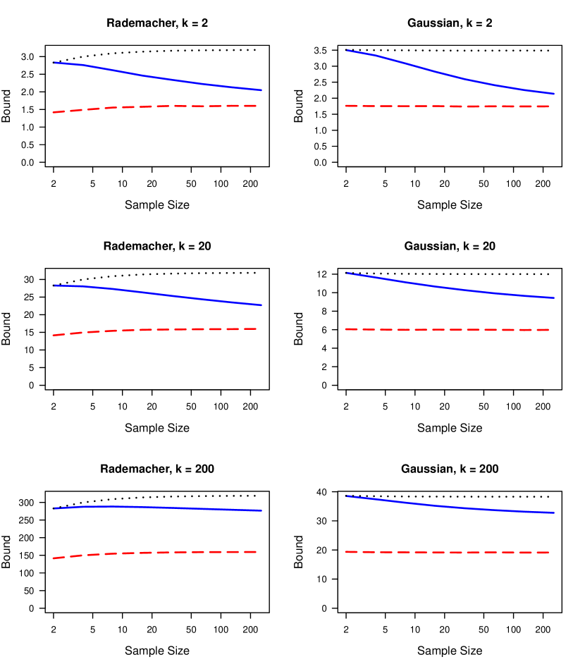
Figure 1: For multivariate Rademacher (left) and Gaussian mixture (right) data, the average $n^{-1/2}\mathrm{E}\lVert\sum_{i=1}^{n}(X_{i}-\mathrm{E}X_{i})\rVert$ (red dashed lines), twice the Rademacher average $2R_{n}=2n^{-1/2}\mathrm{E}\lVert\sum_{i=1}^{n}\varepsilon_{i}(X_{i}-\mathrm{E}X_{i})\rVert$ (black dotted lines), and the bound using the scaled empirical Wasserstein distance, $R_{n}+W_{2}(\mu_{n},\mu_{n}^{-})/\sqrt{2}$ (blue solid lines) were estimated over 10,000 replications. The dimension of the data is $k=\{2,20,200\}$. For the Rademacher setting, the $\ell_{1}$-norm was used. For the Gaussian setting, the $\ell_{2}$-norm was used. As the sample size increases, the Wasserstein term converges to zero thus sharpening the upper bound.

4 Applications

In the following subsections, a collection of applications of the improved symmetrization inequality are detailed. These include a test for data symmetry, the construction of nonasymptotic high dimensional confidence sets, bounding the variance of an empirical process, and Nemirovski’s inequality for Banach space valued random variables.

4.1 Permutation test for data symmetry

In the previous sections, we proposed the Wasserstein distance $W_{2}(\mu,\mu^{-})$ to quantify the symmetry of a measure $\mu$. Now, given $n$ iid observations $X_{1},\ldots,X_{n}$ with common measure $\mu$, we propose a procedure to test for whether or not $\mu$ is symmetric. The bootstrap approach from Section 3 for estimating the empirical Wasserstein distance is applied, and a permutation test is applied to the bootstrapped sample. Note that while the Wasserstein-2 metric is specifically used in our improved symmetrization inequality, for this test, any Wasserstein-$p$ metric can be utilized as is done in the numerical simulations below.

The bootstrap-permutation test proceeds as follows:

1. Choose a number $r$ of bootstrap replications to perform.

2. For each bootstrap replication, permute the data by some uniformly randomly drawn $\rho\in S_{n}$, the symmetric group on $n$ elements.

3. Use the Hungarian algorithm to compute the optimal assignment cost, $\omega_{0}$, between the data sets $\{X_{\rho(1)},\ldots,X_{\rho(n/2)}\}$ and $\{-X_{\rho(n/2+1)},\ldots,-X_{\rho(n)}\}$.

4. Denote this new half-negated data set $Y$ where $Y_{i}=X_{\rho(i)}$ for $i\leq n/2$ and $Y_{i}=-X_{\rho(i)}$ for $i>n/2$.

5. Draw $m$ random permutations $\rho_{1},\ldots\rho_{m}\in S_{n}$. For each $\rho_{i}$, compute $\omega_{i}$, the optimal assignment cost between $\{Y_{\rho_{i}(1)},\ldots,Y_{\rho_{i}(n/2)}\}$ and $\{Y_{\rho_{i}(n/2+1)},\ldots,Y_{\rho_{i}(n)}\}$.

6. Return the p-value, $p_{j}=\#\{\omega_{i}>\omega_{0}\}/m$.

7. Average the $r$ p-values to get an overall p-value, $p=r^{-1}\sum_{j=1}^{r}p_{j}$.

Note that for very large data sets, it may be computationally impractical to find a perfect matching between two sets of $n/2$ nodes as performing this test as stated has a computational complexity of order $O(mn^{3})$. In that case, randomly draw $n^{\prime}<n$ elements from the data set in step 1, draw a $\rho\in S_{n^{\prime}}$, and proceed as before.

This permutation test was applied to simulated multivariate Rademacher data in $\mathbb{R}^{5}$. For sample sizes $n=10$ and $n=100$, let $X_{1},\ldots,X_{n}$ be iid multivariate Rademacher$(p)$ random variables where each $X_{i}$ is comprised of a vector of independent univariate Rademacher$(p)$ random variables. For values of $p\in[0.5,0.8]$, the power of this test was experimentally computed over 1000 simulations. The results are displayed in Figure 2. For the $\ell^{1}$ and $\ell^{2}$ metrics and Wasserstein distances $W_{1}$ and $W_{2}$, the performances of the permutation test were comparable except for the $(\ell^{2},W_{2})$ case, which performed poorer in both the large and small sample size settings. For the large sample size, $n=100$, Mardia’s test for multivariate skewness (Mardia, 1970, 1974) was included, which uses the result that

$$\frac{6}{n}\sum_{i=1}^{n}\sum_{j=1}^{n}\left[{(X_{i}-\bar{X})}^{\mathrm{T}}\hat{\Sigma}^{-1}(X_{j}-\bar{X})\right]^{3}\xrightarrow{\text{d}}\chi^{2}\left(k(k+1)(k+2)/6\right)$$

where $\hat{\Sigma}$ is the empirical covariance matrix of the data. However, this is shown to be less powerful than the proposed permutation test. Furthermore, as this test is asymptotic in design, it gave erroneous results in the $n=10$ case and was thus excluded from the figure.

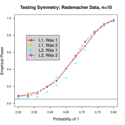
Figure 2: For data in $\mathbb{R}^{5}$, the $\ell^{1}$ and $\ell^{2}$ metrics, and the Wasserstein distances $W_{1}$ and $W_{2}$, the experimentally computed power of the permutation test is plotted for Rademacher$(p)$ data as $p$, the probability of 1, increases thus skewing the distribution. The sample size is $n=100$ on the left plot and is $n=10$ on the right plot. The $n=100$ case includes an asymptotic test for skewness. This test fails in the nonasymptotic $n=10$ case and thus is not included.

4.2 High dimensional confidence sets

A method for constructing nonasymptotic confidence regions for high dimensional data using a generalized bootstrap procedure was proposed in the article of Arlot et al. (2010). Beginning with a sample of independent and identically distributed $Y_{1},\ldots,Y_{n}\in\mathbb{R}^{K}$ and the assumptions that the $Y_{i}$ are symmetric about their mean, i.e. $Y_{i}-\mu\overset{\text{d}}{=}\mu-Y_{i}$, and are bounded in $L_{p}$-norm, i.e. $\lVert Y_{i}-\mu\rVert_{p}\leq M$, they prove, among many other results, that for some fixed $\alpha\in(0,1)$, the following holds with probability $1-\alpha$:

$$\phi\left(\bar{Y}-\mu\right)\leq\left(\frac{n}{n-1}\right)\mathrm{E}_{\varepsilon}\phi\left(\frac{1}{n}\sum_{i=1}^{n}\varepsilon_{i}(Y_{i}-\bar{Y})\right)+\frac{2M}{\sqrt{n}}\sqrt{\log(1/\alpha)}$$

where $\phi:\mathbb{R}^{K}\rightarrow\mathbb{R}$ is a function that is subadditive, positive homogeneous, and bounded by $L_{p}$-norm. By substituting our Theorem 2.6 for their Proposition 2.4 allows us to drop the symmetry condition and achieve a more general $(1-\alpha)$ confidence region.

Proposition 4.1.

For a fixed $\alpha\in(0,1)$ and $p\in[1,\infty]$, let $\phi:\mathbb{R}^{k}\rightarrow\mathbb{R}$ be subadditive, positive homogeneous, and bounded in $L_{p}-$norm. Then, for some $M>0$, the following holds with probability at least $1-\alpha$.

$$\phi\left(\bar{Y}-\mu\right)\leq\mathrm{E}_{\varepsilon}\phi\left(\frac{1}{n}\sum_{i=1}^{n}\varepsilon_{i}(Y_{i}-\bar{Y})\right)+(2n)^{-1/2}\left({2\sqrt{2}M}\sqrt{\log(1/\alpha)}+W_{2}(\mu,\mu^{-})\right).$$

4.3 Bounds on empirical processes

Symmetrization arises when bounding the variance of an empirical process. In Boucheron et al. (2013), the following result is stated as Theorem 11.8 and is subsequently proved using the original symmetrization inequality resulting in suboptimal coefficients.

Theorem 4.2 (Boucheron et al. (2013), Theorem 11.8).

For $i\in\{1,\ldots,n\}$ and $s\in\mathcal{T}$, a countable index set, let $X_{i}=(X_{i,s})_{s\in\mathcal{T}}$ be a collection of real valued random variables. Furthermore, let $X_{1},\ldots,X_{n}$ be independent. Assume $\mathrm{E}X_{i,s}=0$ and $\lvert X_{i,s}\rvert\leq 1$ for all $i=1,\ldots,n$ and for all $s\in\mathcal{T}$. Defining $Z=\sup_{s\in\mathcal{T}}\sum_{i=1}^{n}X_{i,s}$, then

$$\mathrm{Var}\left(Z\right)\leq 8\mathrm{E}Z+2\sigma^{2}$$

where $\sigma^{2}=\sup_{s\in\mathcal{T}}\sum_{i=1}^{n}\mathrm{E}X_{i,s}^{2}$.

The given proof uses the symmetrization inequality twice as well as the contraction inequality (see Ledoux and Talagrand (1991) Theorem 4.4, and Boucheron et al. (2013) Theorem 11.6) to establish the bounds

$$\mathrm{E}\sup_{s\in\mathcal{T}}\sum_{i=1}^{n}X_{i,s}^{2}\leq\sigma^{2}+2\mathrm{E}\sup_{s\in\mathcal{T}}\sum_{i=1}^{n}\varepsilon_{i}X^{2}_{i,s}~{}~{}\text{ and }~{}~{}\mathrm{E}\sup_{s\in\mathcal{T}}\sum_{i=1}^{n}\varepsilon_{i}X^{2}_{i,s}\leq 4\mathrm{E}Z.$$

Making use of the improved symmetrization inequality cuts the coefficient of $\mathrm{E}Z$ by a factor of 4 to the tighter

$$\mathrm{Var}\left(Z\right)\leq 2\mathrm{E}Z+2\sigma^{2}+O(\sqrt{n}).$$

Beyond this textbook example of bounding the variance of an empirical process, symmetrization arguments are used to construct confidence sets for empirical processes in Giné and Nickl (2010); Lounici and Nickl (2011); Kerkyacharian et al. (2012); Fan (2011). The coefficients in all of their results can be similarly improved using the improved symmetrization inequality.

4.4 Type, Cotype, and Nemirovski’s Inequality

In the probability in Banach spaces setting, let $X_{i}\in(B,\lVert\cdot\rVert)$ for $i=1,\ldots,n$ be a collection of independent mean zero Banach space valued random variables. A collection of results referred to as Nemirovski inequalities (Nemirovski, 2000; Dümbgen et al., 2010) are concerned with whether or not there exists a constant $K$ depending only on the norm such that

$$\mathrm{E}\left\lVert\sum_{i=1}^{n}X_{i}\right\rVert^{2}\leq K\sum_{i=1}^{n}\lVert X_{i}\rVert^{2}.$$

For example, in the Hilbert space setting, orthogonality allows for $K=1$ and the inequality can be replaced by an equality.

One such result requires the notion of type and cotype. A Banach space $(B,\lVert\cdot\rVert)$ is said to be of Rademacher type $p$ for $1\leq p<\infty$ (respectively, of Rademacher cotype $q$ for $1\leq q<\infty$) if there exists a constant $T_{p}$ (respectively, $C_{q}$) such that for all finite non-random sequences $(x_{i})\in B$ and $(\varepsilon_{i})$, a sequence of independent Rademacher random variables,

$$\mathrm{E}\left\lVert\sum_{i}\varepsilon_{i}x_{i}\right\rVert^{p}\leq T_{p}^{p}\sum_{i}\lVert x_{i}\rVert^{p},~{}~{}\left(\text{respectively, }\sum_{i}\lVert x_{i}\rVert^{q}\leq C_{q}^{-q}\mathrm{E}\left\lVert\sum_{i}\varepsilon_{i}x_{i}\right\rVert^{q}\right).$$

These definitions and the original symmetrization inequality lead to the following proposition.

Proposition 4.3 (Ledoux and Talagrand (1991) Proposition 9.11, Dümbgen et al. (2010) Proposition 3.1).

Let $X_{i}\in B$ for $i=1,\ldots,n$ and $S_{n}=n^{-1}\sum_{i=1}^{n}X_{i}$. If $(B,\lVert\cdot\rVert)$ is of type $p\geq 1$ with constant $T_{p}$ (respectively, of cotype $q\geq 1$ with constant $C_{q}$), then

$$\mathrm{E}\lVert S_{n}\rVert^{p}\leq(2T_{p})^{p}n^{-p}\sum_{i=1}^{n}\mathrm{E}\lVert X_{i}\rVert^{p},~{}~{}\left(\mathrm{E}\lVert S_{n}\rVert^{q}\geq(2C_{q})^{-q}n^{-q}\sum_{i=1}^{n}\mathrm{E}\lVert X_{i}\rVert^{q}\right)$$

The proposition can be refined by applying our improved symmetrization inequality along with the Rademacher type $p$ condition if the $X_{i}$ are additionally norm bounded. If the $X_{i}$ have a common law $\mu$, let $W_{2}=W_{2}(\mu,\mu^{-})$ be the Wasserstein distance between $\mu$ and its reflection.

Proposition 4.4.

Under the setting of Proposition 4.3, additionally assume that $\lVert X_{i}\rVert\leq 1$ for $i=1,\ldots,n$. Then,

$$\mathrm{E}\lVert S_{n}\rVert^{p}\leq T_{p}^{p}n^{-p}\sum_{i=1}^{n}\mathrm{E}\lVert X_{i}\rVert^{p}+\frac{pW_{2}}{\sqrt{2n}},~{}~{}\left(\mathrm{E}\lVert S_{n}\rVert^{q}\geq C_{q}^{-q}n^{-q}\sum_{i=1}^{n}\mathrm{E}\lVert X_{i}\rVert^{q}-\frac{qW_{2}}{\sqrt{2n}}\right)$$

Proof.

In the context of Theorem 2.6, set $\psi(\cdot)=\lVert\cdot\rVert^{p}$. Given the bound $\lVert X_{i}\rVert\leq 1$, we have that $\lVert\psi\rVert_{Lip}=p$. Scale by $p$, and the first result follows. ∎

Note that for identically distributed $X_{i}\in B$, the order of the original bound for a type $p$ Banach space is $O(n^{1-p})$ while the Wasserstein correction term is $O(n^{-1/2})$. This correction will give an obvious benefit for spaces of type $p<3/2$. However, even for spaces of type 2, the new bound can be tighter specifically in the high dimensional setting when $d\gg n$. Indeed, consider $\ell_{\infty}(\mathbb{R}^{d})$, which is discussed in particular in Section 3.2 of Dümbgen et al. (2010) where it is shown to be of type 2 with constant $T_{p}=\sqrt{2\log(2d)}$. For iid $X_{i}\in\ell_{\infty}(\mathbb{R}^{d})$, the bounds to compare are

$$\frac{8\log(2d)}{n}\mathrm{E}\lVert X_{i}\rVert_{\infty}^{2}~{}~{}~{}\text{ and }~{}~{}~{}\frac{2\log(2d)}{n}\mathrm{E}\lVert X_{i}\rVert_{\infty}^{2}+\sqrt{\frac{2}{n}}W_{2}(\mu,\mu^{-}).$$

Figure 3 displays such a comparison for $n=10$, $d\in\{5,25,50\}$, and iid $X_{i,j}+\alpha/(1+\alpha)\sim\mathrm{Beta}\left(\alpha,1\right)$ for $i=1,\ldots,n$ and $j=1,\ldots,d$. Hence, the $X_{i}$ are Beta random variables that are shifted to have zero mean. $W_{2}(\mu,\mu^{-})$ is approximated by $\mathrm{E}W_{2}(\mu_{5},\mu_{5}^{-})$, which is computed via the bootstrap procedure outlined in Section 3. The new bound can be seen to have better performance than the old one specifically in the cases of $d=25$ and $d=50$ when $\alpha$ is not too large.

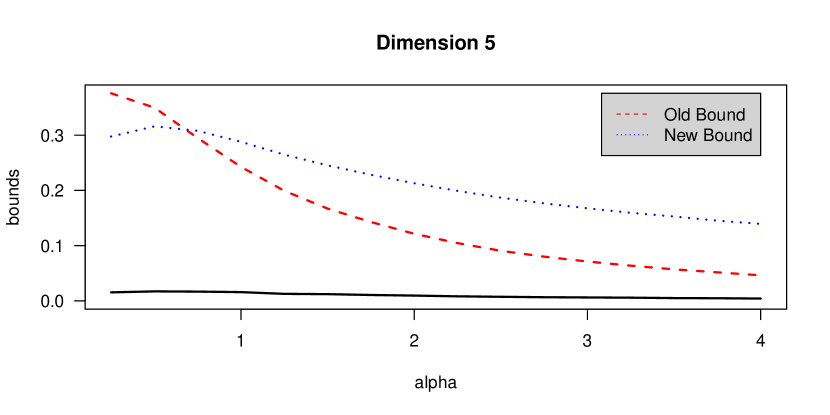
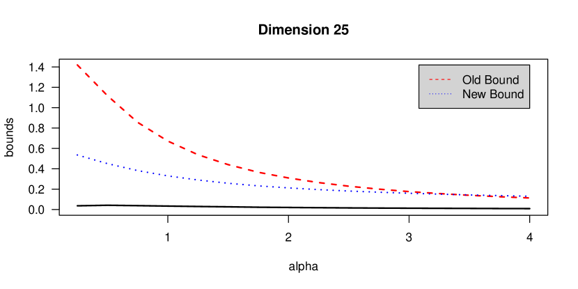
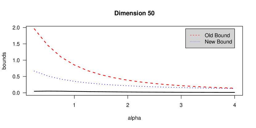
Figure 3: A comparison of the old bound from Proposition 4.3, the red dashed line, and the new bound from Proposition 4.4, the blue dotted line, for a sample $n=10$ $X_{i}\in\ell_{\infty}(\mathbb{R}^{d})$ for dimensions $d\in\{5,25,50\}$. Each $X_{i}=(X_{i,1},\ldots,X_{i,d})$ where each $X_{i,j}+\alpha/(1+\alpha)\overset{\text{iid}}{\sim}\mathrm{Beta}\left(\alpha,1\right)$. The solid black line indicates the left hand side in the two propositions of $\mathrm{E}\lVert S_{n}\rVert_{\infty}^{2}$.

4.4.1 A Nemirovski variant with weak variance

As one further example of improved symmetrization, a variation of Nemirovski’s inequality found in Section 13.5 of Boucheron et al. (2013) is proved via a similar symmetrization argument for the $\ell_{p}$ norm with $p\geq 1$. Let $X_{1},\ldots,X_{n}\in\mathbb{R}^{d}$ be independent mean zero random variables. Let $B_{q}=\{x\in\mathbb{R}^{d}:\lVert x\rVert_{q}\leq 1\}$, and define the weak variance $\Sigma_{p}^{2}=n^{-2}\mathrm{E}\sup_{t\in B_{q}}\sum_{i=1}^{n}\left\langle t,X_{i}\right\rangle^{2}$. The resulting inequality is

$$\mathrm{E}\lVert S_{n}\rVert^{2}_{p}\leq 578d\Sigma_{p}^{2}.$$

Replacing the old symmetrization inequality with the improved version reduces the coefficient of 578 roughly by a factor of 4 resulting in

$$\mathrm{E}\lVert S_{n}\rVert^{2}_{p}\leq 146d\Sigma_{p}^{2}+O(n^{-1/2}).$$

5 Discussion

The symmetrization inequality is a fundamental result for probability in Banach spaces, concentration inequalities, and many other related areas. However, not accounting for the amount of asymmetry in the given random variables has led to pervasive powers of two throughout derivative results. Our improved symmetrization inequality incorporates such a quantification of asymmetry through use of the Wasserstein distance. Besides being theoretically sound, it is shown in simulations to provide a tightness superior to that of the original result. Going beyond the inequality itself, this Wasserstein distance offers a novel and powerful way to analyze the symmetry of random variables or lack thereof. It can and should be applied to countless other results that were not considered in this current work.

Appendix A Past results used

Lemma A.1 ( Kantorovich-Rubinstein Duality, see Villani (2008) ).

Under the setting of Definition 2.1,

$$W_{1}(\mu,\nu)=\sup_{\lVert\phi\rVert_{Lip}\leq 1}\left\{\int_{\mathcal{X}}\phi d\mu-\int_{\mathcal{X}}\phi d\nu\right\}.$$

Lemma A.2.

Under the setting of Definition 2.1, for $p<q$,

$$W_{p}(\mu,\nu)\leq W_{q}(\mu,\nu).$$

Proof.

Jensen or Hölder’s Inequality ∎

Lemma A.3 ( Convolution property of $W_{2}$, see Bickel and Freedman (1981) ).

For Hilbert space valued random variables $X_{i}$ with law $\mu_{i}$ and $Y_{i}$ with law $\nu_{i}$ for $i=1,\ldots,n$, define $\mu^{*n}$ to be the law of $\sum_{i=1}^{n}X_{i}$ and similarly for $\nu^{*n}$. Then,

$$W_{2}^{2}(\mu^{*n},\nu^{*n})\leq\sum_{i=1}^{n}W_{2}^{2}(\mu_{i},\nu_{i}).$$

Lemma A.4 ( Convergence of Empirical Measure, see Bickel and Freedman (1981) ).

Let $X_{1},\ldots,X_{n}$ be independent and identically distributed Banach space valued random variables with common law $\mu$. Let $\mu_{n}$ be the empirical distribution of the $X_{i}$. Then,

$$W_{p}(\mu_{n},\mu)\rightarrow 0,~{}~{}\text{as }n\rightarrow\infty.$$

References

- Ahuja et al. (1993) Ravindra K. Ahuja, Thomas L. Magnanti, and James B. Orlin. Network Flows: Theory, Algorithms, and Applications. Prentice-Hall, Inc, 1993.
- Arlot et al. (2010) Sylvain Arlot, Gilles Blanchard, and Etienne Roquain. Some nonasymptotic results on resampling in high dimension, i: confidence regions. The Annals of Statistics, 38(1):51–82, 2010.
- Bickel and Freedman (1981) Peter J Bickel and David A Freedman. Some asymptotic theory for the bootstrap. The Annals of Statistics, pages 1196–1217, 1981.
- Boucheron et al. (2013) Stéphane Boucheron, Gábor Lugosi, and Pascal Massart. Concentration inequalities: A nonasymptotic theory of independence. Oxford University Press, 2013.
- Dümbgen et al. (2010) Lutz Dümbgen, Sara A van de Geer, Mark C Veraar, and Jon A Wellner. Nemirovski’s inequalities revisited. American Mathematical Monthly, 117(2):138–160, 2010.
- Efron and Stein (1981) Bradley Efron and Charles Stein. The jackknife estimate of variance. The Annals of Statistics, pages 586–596, 1981.
- Fan (2011) Zhou Fan. Confidence regions for infinite-dimensional statistical parameters. Part III essay in Mathematics, University of Cambridge, 2011. http://web.stanford.edu/ zhoufan/PartIIIEssay.pdf.
- Fournier and Guillin (2015) Nicolas Fournier and Arnaud Guillin. On the rate of convergence in wasserstein distance of the empirical measure. Probability Theory and Related Fields, 162(3-4):707–738, 2015.
- Giné and Nickl (2010) Evarist Giné and Richard Nickl. Adaptive estimation of a distribution function and its density in sup-norm loss by wavelet and spline projections. Bernoulli, 16(4):1137–1163, 2010.
- Giné and Zinn (1984) Evarist Giné and Joel Zinn. Some limit theorems for empirical processes. The Annals of Probability, 12(4):929–989, 1984.
- Kerkyacharian et al. (2012) Gerard Kerkyacharian, Richard Nickl, and Dominique Picard. Concentration inequalities and confidence bands for needlet density estimators on compact homogeneous manifolds. Probability Theory and Related Fields, 153(1-2):363–404, 2012.
- Koltchinskii (2006) Vladimir Koltchinskii. Local rademacher complexities and oracle inequalities in risk minimization. The Annals of Statistics, 34(6):2593–2656, 2006.
- Kuhn (1955) Harold W Kuhn. The hungarian method for the assignment problem. Naval research logistics quarterly, 2(1-2):83–97, 1955.
- Ledoux and Talagrand (1991) Michel Ledoux and Michel Talagrand. Probability in Banach Spaces: isoperimetry and processes, volume 23. Springer, 1991.
- Lounici and Nickl (2011) Karim Lounici and Richard Nickl. Global uniform risk bounds for wavelet deconvolution estimators. The Annals of Statistics, 39(1):201–231, 2011.
- Mardia (1970) Kanti V Mardia. Measures of multivariate skewness and kurtosis with applications. Biometrika, 57(3):519–530, 1970.
- Mardia (1974) Kanti V Mardia. Applications of some measures of multivariate skewness and kurtosis in testing normality and robustness studies. Sankhyā: The Indian Journal of Statistics, Series B, pages 115–128, 1974.
- Nemirovski (2000) Arkadi Nemirovski. Topics in non-parametric. Ecole d’Eté de Probabilités de Saint-Flour, 28:85, 2000.
- Panchenko (2003) Dmitry Panchenko. Symmetrization approach to concentration inequalities for empirical processes. Annals of Probability, pages 2068–2081, 2003.
- Rhee and Talagrand (1986) WanSoo T Rhee and Michel Talagrand. Martingale inequalities and the jackknife estimate of variance. Statistics & probability letters, 4(1):5–6, 1986.
- Steele (1986) J Michael Steele. An Efron-Stein inequality for nonsymmetric statistics. The Annals of Statistics, pages 753–758, 1986.
- Steele (1997) J Michael Steele. Probability theory and combinatorial optimization, volume 69. Siam, 1997.
- Villani (2008) Cédric Villani. Optimal transport: old and new, volume 338. Springer Science & Business Media, 2008.