A bootstrap-based method to estimate directional extreme risk regions at high levels
Abstract
In multivariate extreme value theory (MEVT), the focus is on analysis outside of the observable sampling zone, which implies that the region of interest is associated to high risk levels. This work provides tools to include directional notions into the MEVT, giving the opportunity to characterize the recently introduced directional multivariate quantiles (DMQ) at high levels. Then, an out-sample estimation method for these quantiles is given. A bootstrap procedure carries out the estimation of the tuning parameter in this multivariate framework and helps with the estimation of the DMQ. Asymptotic normality for the proposed estimator is provided and the methodology is illustrated with simulated data-sets. Finally, a real-life application to a financial case is also performed.
1 Introduction
The estimation of extreme level curves is important for identifying extreme events and for characterizing the joint tails of multidimensional distributions. They are usually considered as quantiles at high levels; that is, they are linked with a probability of occurrence of certain event, where is a very small number. This proposal considers a non-parametric approach for values of lower or equal than , where denotes the sample size. This implies that the number of data points that fall beyond the quantile curve is small and can even be zero, thus we are outside of the observable sample zone, or in other words, in the out-sample estimation framework. This lack of relevant data points makes the estimation difficult, making it necessary to introduce tools from the multivariate extreme value theory (MEVT).
The main purpose of this paper is to provide an extension of the by introducing the directional approach and also to give an out-sample estimation method for the directional multivariate quantiles (DMQ) introduced in [Torres et al.(2015)] and [Torres et al.(2016)]. In these papers, the directional setting refers to the inclusion of a parameter of direction that allows analysis of data by looking at the cloud of observations from different perspectives. Accurate assessments of these quantiles are sought in a diversity of applications from financial risk management (e.g. [Torres et al.(2015)]) to environmental impact assessment (e.g. [Torres et al.(2016)]). A non-parametric estimation method was developed in [Torres et al.(2015)] to estimate the directional quantile based on the empirical probability distribution, which is valid just for the in-sample scenario; that is .
Both scenarios, in-sample and out-sample, have been widely studied in the univariate setting and recently the literature has focused on the extension to the multivariate context. Some relevant references in this area can be grouped into three categories as follows. Firstly, estimation under optimization processes, for instance, based on optimization over linear quantile regression (see, e.g., [Chaudhuri (1996), Hallin et al.(2010), Mukhopadhyay and Chatterjee (2011), Kong and Mizera (2012), Girard and Stupfler (2015)]). In this case, an example of the in-sample framework is given by [Chaudhuri (1996)] for geometric quantiles. [Girard and Stupfler (2015)] also proposed an out-sample estimation method for geometric quantiles.
A second category contains methods determining level curves of joint density functions in such a way that the set of points outside those contours has a probability equal to a given level . These methods easily describe inner and outer regions at the given level and inherently cover the infinite set of directions through those contours (e.g., [Cai et al.(2011), Einmahl et al.(2013)]). The estimators proposed in this category have been developed mainly for the out-sample framework. For instance, [Cai et al.(2011)] provided estimation of bivariate contour levels for some joint densities with elliptical and non-elliptical distributions, considering cases with asymptotic dependence and asymptotic independence. Other methodologies in this category are based on the trimming through depth functions. [Serfling (2002)] described in-sample methods considering different depth functions and [He and Einmahl (2017)] presented an out-sample contour estimation based on the Tukey depth.
Last category considers level curve estimations using either joint distribution or survival functions (e.g. [De Haan and Huang (1995), Fernández-Ponce and Suárez-Llorens (2002), Belzunce et al.(2007), Chebana and Ouarda (2009), Di Bernardino et al.(2011)]). Works based on copulas are also classified in this group (e.g. [Chebana and Ouarda (2011), Durante and Salvadori (2010), Salvadori et al.(2011), Binois et al.(2015)]). These works have introduced the estimation procedures in both contexts, in-sample and out-sample, but most of them present the theory and related applications only in the bivariate case. Since the proposal developed in this work is somehow based on distributions, it belongs to this third category.
As we have mentioned before, the methodology developed in this work includes a directional notion and we want to highlight its importance in our contribution. One can find in the literature a few references dealing with this notion. [Chaudhuri (1996)] is one of the first works that includes directions. However, this multivariate aspect starts to take importance just in the past decade, where an accurate assessment of risk regions arises in a diversity of applications. For instance, [Embrechts and Puccetti (2006)] studied bounds for multivariate financial risks, highlighting the usefulness of analysis considering two particular directions. [Belzunce et al.(2007)] presented a bivariate quantile application to air quality where the directions are related to the four classical orthants.
Other examples describing the importance of directions are [Hallin et al.(2010)], where it was proposed directional projections to show a relationship between their quantile trimming and the trimming obtained through the Tukey depth. [Kong and Mizera (2012)] used a similar idea to build multivariate growth chart applications. [Fraiman and Pateiro-López (2012)] provided a directional projection-based definition for infinite-dimensional multivariate quantiles in Hilbert spaces. In financial risk management [Torres et al.(2015)] showed the advantage of using the portfolio weights of investment as the direction of analysis to provide an upper bound for the maximum loss. [Torres et al.(2016)] performed an application to environmental impact assessment, where it can be seen the improvement of identifying extremes by using the first principal component as a direction of analysis.
Therefore, inspired by [De Haan and Huang (1995)] where an out-sample estimator for bivariate level curves of a distribution function was established, the contribution in this paper is threefold: 1) to include the directional framework given in [Torres et al.(2015), Torres et al.(2016)] in the MEVT analysis, 2) to establish an estimator those directional high level quantiles in a general dimension and 3) to provide a non-parametric estimation method for these high level directional quantiles and some asymptotic results.
The paper is organized as follows. In Section 2 we summarize the main definitions and results related to the directional framework used in the paper. Section 3 introduces definitions from the multivariate extreme theory to fix conditions over the random vector that allow to ensure the results under the directional framework. In Section 3.1, we describe the characterization of the elements of the DMQ at high levels, based on the heuristic ideas in [De Haan and Huang (1995)]. Section 4 develops statistical tools to perform an out-sample estimation of the DMQ. The high level estimator is introduced in Section 4.1. Asymptotic normality of this estimator is presented in Section 4.2. Later on, we adapt a bootstrap-based method to deal with the tuning parameter. Section 5 illustrates the performance of our multivariate estimation procedure (in dimensions and ) in a multivariate distribution case. Section 6 presents a directional analysis over daily filtered returns of three different international indices. Finally, in Section 7 some conclusions and perspectives are provided. Proofs and auxiliary results are postponed to Appendix A.
2 Directional multivariate quantiles
This section introduces the preliminary definitions and notation necessary to understand the contributions of the paper. Our directional multivariate setting is based on the work developed in [Laniado et al.(2012)]. Firstly, we recall the notion of oriented orthant.
Definition 2.1 (Oriented orthant).
An oriented orthant in with vertex in direction is defined by,
where and is an orthogonal matrix such that , with .
Note that an oriented orthant is a translation by and rotation by of the non-negative Euclidean orthant. [Torres et al.(2015)] pointed out that is not unique for . Hence, in order to guarantee uniqueness, they stated the following. Let be a unit vector with non-null components and let and be matrices defined as,
where , is the th component of , is the scalar sign function and is the th column of the identity matrix. Then and have full rank and unique QR decomposition,
such that , are triangular matrices with positive diagonal elements and , are the correspondent orthogonal matrices (see [Horn and Johnson (2013)][Theorem 2.1.14, p.g. 89]). Therefore, [Torres et al.(2015)] defined the QR oriented orthant as follows.
Definition 2.2 (QR oriented orthant).
The QR oriented orthant with vertex in direction , denoted as , is the oriented orthant satisfying .
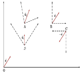
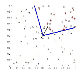
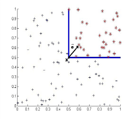
Figure 1 illustrates the QR oriented orthant in Definition 2.2 for different vertexes and directions. One can observe that the mass accumulated inside a QR oriented orthant with vertex and direction corresponds to the probability of such orthant and moreover, it is equivalent to evaluate the vertex in the survival function of the rotated random vector . We remark that directions with non-null components is not a restrictive assumption, because if there exists a direction with zero in one or more components, this implies independence of the corresponding marginals from the joint extreme behavior of interest.
Also, quantiles at certain level in direction have been defined in [Torres et al.(2015)] as follows.
Definition 2.3 (Directional multivariate quantile (DMQ)).
Let be a random vector with associated probability distribution . Then the directional multivariate quantile at level in direction is defined as
| (2.1) |
where denotes the boundary of the considered set and .
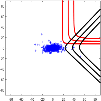
Examples of the previous definition applied on a multivariate distribution are given for high levels of in different directions in Figure 2 (dimension ) and Figure 9 (dimension ). In the univariate setting, extremes are analyzed considering the two possibilities of exceeding from either distributions or survival functions and most of the extensions of these analyses to the multivariate setting have also been concentrated on these two types of exceeding. The interested reader is referred to [Shiau (2003), Salvadori (2004), Embrechts and Puccetti (2006)] for extensions on the bivariate case and also to [Gupta and Manohar (2005), Cousin and Di Bernardino (2013), Di Bernardino et al.(2015)] for some generalized multivariate versions.
However, the multivariate setting offers infinite possibilities of exceeding to be considered and our directional framework explores these alternatives. First, note that Definition 2.3 provides a multivariate quantile based on two free parameters: traditional level and a unit vector of direction . Given the out-sample framework of this paper, the level will be considered lower or equal than for a sample size , but more important is to highlight that the parameter of direction is completely free and each choice implies different hyper-curves, each of those focusing on the extreme behavior of in particular areas of its support. Note that the possibilities based on the distributions and the survival functions of a random vector are provided through the directions , respectively. Hereafter we will call these directions: classical directions.
Second, we point out that there are other interesting directions to be taken into consideration. For instance in portfolio optimization, the direction given by the portfolio weights of investments is of particular interest because it takes into account the losses due to the composition of the investment in a portfolio (see [Laniado et al.(2012), Torres et al.(2015)]). In environmental phenomena, the directional approach has also been applied to detect extreme events by considering the direction of maximum variability of the data (see [Torres et al.(2016)]). In summary, different contexts or phenomena could suggest different particular directions either by external information or other causes, so the direction is a parameter to be chosen by a practitioner helping to capture the overall behavior of the data and to improve the visualization of results.
3 Directional MEVT: A probabilistic approach
In this section, we introduce conditions over in order to extend classic MEVT by using the directional framework in Section 2. This allows us to provide a general theory that includes a free parameter of direction . Those conditions involve notions of multivariate regular variation. The interested reader is referred to [Resnick (1987), De Haan and Ferreira (2006), Resnick (2007)].
Assumption A1.
The support of is all .
This assumption is introduced to guarantee that, independently of the chosen direction , possesses a part of its support on the positive orthant. Indeed if has a bounded support, one should be aware of the fact that many directions become uninformative in terms of maximums. Then, if Assumption A1 is not satisfied, it is advisable to fix first the desired direction and then to make the corresponding analysis in terms of classical MEVT for the vector .
We now characterize the right tail behavior of (see Assumption A2) and later we show that this characterization is inherited for any rotation of the random vector (see Proposition 3.2).
Definition 3.1 (First order multivariate regular variation).
A random vector has first order multivariate regular variation with tail index , if there exists a real-value function that is regularly varying at infinity111A function , if it holds that , for all . with exponent , denoted by , and a non-zero measure on the Borel field , such that, if ,
| (3.1) |
where means vague convergence (see, e.g., [Jessen and Mikosh (2006), Resnick (1987)]).
If verifies Definition 3.1 with , then it is called a heavy tailed random vector and the measure of convergence in (3.1) has the homogeneity property of order , i.e., , for all and every Borel set .
Assumption A2.
has first order multivariate regular variation with tail index .
Note that Assumption A2 is a stronger condition than belonging to a multivariate max-domain of attraction (see [De Haan and Ferreira (2006)]). Indeed, as it is mentioned in [Resnick (1987)][Remark 6.1], A2 implies tail equivalence among marginal distributions, reducing all marginal tail indexes to . In practice, tails could be different and in this case, there are some techniques to overcome this flaw. (see for instance [Resnick (1987)][Section 6.5.6]). We refer to Remark 1 below for further comments on this point.
Proposition 3.2.
If satisfies Assumption A2 with tail index , then the random vector has first order multivariate regular variation with tail index , for any orthogonal transformation .
Proposition 3.2 is a special case of Proposition A.1 in [Basrak et al.(2002)] for a deterministic matrix . An alternative proof of Proposition 3.2 is given in Appendix A.
Definition 3.3 (Second order multivariate regular variation).
A random vector has second order multivariate regular variation with indexes , if there exist functions and , such that , ; satisfying,
locally uniformly for all relatively compact rectangles , where is not identically zero. (see [Resnick (2002)]).
Assumption A3.
has second order multivariate regular variation with indexes .
Proposition 3.4.
If satisfies Assumption A3 with indexes , then the random vector has second order regular variation with indexes , for any orthogonal transformation .
Proof of Proposition 3.4 is given in Appendix A. Assumption A3 will be crucial in Section 4.2 to prove asymptotic normality for the proposed estimator of the DMQ. From now on, we consider that a random vector satisfies Assumptions A1-A3.
3.1 Characterization of the DMQ at high levels
The aim of this paragraph is to characterize the points belonging to in Definition 2.3 for small values of the level, (). Our proposal is based in two main aspects. The first one is the quasi-orthogonal invariace property given in [Torres et al.(2015)][Property 3.8], i.e.,
| (3.2) |
and the second one is referred to the heuristic ideas of the bivariate quantile parameterization given in [De Haan and Huang (1995)] extended to a general directional multivariate context.
Let be the distribution function of the random vector . Note that is the set of points such that,
Furthermore, Proposition 3.2 implies that belongs to the max-domain of attraction of a non-degenerate multivariate extreme value distribution with the same Frechét marginals (the latter given the tail equivalence among marginal distributions see [Resnick (1987)][Chapter 5]). Moreover, there exist two sequences , such that,
| (3.3) |
In addition, a direct consequence of (3.3) is that each marginal of has the form , for (see also [De Haan and Ferreira (2006)][Chapter 6]). Hence, it is possible to write,
| (3.4) |
where is the marginal of . Thus, (3.4) implies that for small values of , the quantile related to verifies the following relationship,
| (3.5) |
Now, to obtain the joint behavior characterizing the elements belonging to , we introduce the bivariate heuristic ideas in [De Haan and Huang (1995)] based on a parameterizable scalar function that approximates such joint quantile structure by a deformation of the marginal quantiles. Then, we first recall that any point can be written alternatively in polar coordinates as , where and belonging to the unit dimensional ball (for a further discussion see [Driver (2003)][pg. 217]). Note also that Assumption A1 expressed in terms of the polar parameterization becomes in the analysis of upper-end points when is such that , for all .
Now, any point of under polar parameterization will be denoted by , where . Finally, we can write the following heuristic for the elements of ,
| (3.6) |
It is crucial to remark the difference between given in (3.5) and in (3.6). The former is related to the univariate quantile of the marginal and the latter is the component of an element in . Therefore, except for , all the elements in (3.6) are known or can be estimated. Then, the problem of estimating turns into the problem of finding a mathematical expression for the scalar function . From (3.3) and (3.6), we obtain
| (3.7) | ||||
Last equality in (3.7) is due to the homogeneity property of (see [De Haan and Ferreira (2006)] [Theorem 6.1.9]).
Hence, from (3.7), we achieve a expression of by approximation. This expression will be denoted as
| (3.8) |
which implies the approximation of given by
| (3.9) |
Thus, is approximated at high levels by the parameterization,
| (3.10) |
where . Thus, by using previous characterizations one can get an out-sample estimator for , which is the objective of next section.
Remark 1.
Note that the analysis provided in this section by using Assumptions A1-A3 makes the characterization feasible independently of the chosen direction . However, if A2 does not hold, but for some direction , belongs to a multivariate max-domain of attraction, then the results of [De Haan and Huang (1995)] for a general dimension , can be directly applied for the transformed vector.
Conversely, our aim here is to develop a general directional theory where under the considered Assumptions A1-A3, practitioners have: (1) to test the regular variation only once for the original random vector and (2) the capacity to look at the data with different perspectives of analysis or even to apply an overall analysis, similar to those provided by density function or depth function approaches, by moving in all its domain.
4 Inference for DMQ at high-levels
For any direction , let be independent and identically distributed (i.i.d.) random vectors, distributed as and denote by the collection of the corresponding th order statistics for each marginal.
Marginal order statistics are important since they allow Equation (3.3) to be written in terms of a subsample that provides significant information about the tail behavior of the joint distribution (see [De Haan and Ferreira (2006)][Section 7.2]). This subsample is related to a tuning intermediate sequence , as . This crucial sequence leads to the break point from which the information of an ordered sample starts to be considered in the tail of the distribution. Then, we obtain,
We now introduce an estimator of (see Section 4.1) and we provide its asymptotic normality (see Section 4.2). Furthermore, we describe a bootstrap based methodology to find an optimal solution of the tuning parameter in our multivariate approach (see Section 4.3).
Notice that due to Proposition 3.2, Proposition 3.4 and the quasi-orthogonal property in Equation (3.2), all the results in the present section are fulfilled independently from the choice of . However, as we mentioned in Remark 1, if we allow to lose the generality of the directional approach and we fix the direction beforehand. Then, we could ask for the random vector to belong to a multivariate max-domain of attraction and we fall on the extension of the work in [De Haan and Huang (1995)] removing the tail equivalence for marginal distributions.
4.1 Directional multivariate quantile estimator
Note that if one has estimators for all the elements in (3.9), an estimator of (3.10) can be provided. For the estimation of the tail index , one can consider a steps procedure. Firstly, the multivariate regular variation condition in Assumption A2 can be tested using the procedure described in [Einmahl and Krajina (2016)]. This ensure the statistical equality of all the marginal tail indexes.
Secondly, each marginal estimation can be done through the moments estimators given in [Dekkers et al.(1989)], i.e.,
| (4.1) |
where .
Notice that each depends on the sample size and the tuning parameter . In Section 4.3, we discuss how to find an optimal selection of based on a joint estimation of the marginal tail indexes.
The estimators for the components of the sequences , can be defined as in [De Haan and Huang (1995)] by
| (4.2) | ||||
| (4.3) |
4.2 Asymptotic normality of
We prove in the following the point-wise asymptotic normality of in (4.6), when , as . Firstly, in our setting, one can get
where , means convergence in distribution, means a component-wise product, means the vector of partial derivatives of a function; , and are such that,
where
is a zero-mean Gaussian random field with covariance function (see [De Haan and Resnick (1993)]),
and is the finite measure provided by Proposition 3.2, such that, . Moreover, from Proposition 4.1 in [De Haan and Resnick (1993)], one can see that the joint distribution of is a multivariate Gaussian distribution. Thus, we can prove the following central limit theorem.
Proposition 4.1 (Point-wise asymptotic normality for ).
Let . Suppose that satisfies Assumption A3 and for the following strong marginal second order condition holds
Assume that
where , , are as in Definition 3.3 and .
Then, for ,
converges in distribution to
Proof of Proposition 4.1 is given in Appendix A. Finally, in Corollary 4.2 below, the point-wise asymptotic normality of is derived since the orthogonal transformations preserve the result in Proposition 4.1.
Corollary 4.2 (Point-wise asymptotic normality for ).
The point-wise asymptotic normality property of the estimator is preserved under orthogonal transformations. Therefore the quasi-orthogonal property in (4.6) implies the point-wise asymptotic normality of .
4.3 Bootstrap method to estimate the tuning parameter
From Equations (4.1)-(4.4), one can appreciate the key role of sequence . However, it is not an easy task to establish optimal tuning parameter for a given sample size . This tuning parameter is complicated to tackle in practice and methods to provide optimality are still a matter of research and discussion.
In the recent literature, one can find only heuristic guidelines adapted to each multivariate application (e.g. [Cai et al.(2011), Cai et al.(2015), Di Bernardino and Palacios-Rodríguez (2016)]), where the selection of parameters such as are mostly based on the identification of a common region of stability across the estimation of particular marginal elements such as marginal tail indexes. For instance, can be selected through a graphical visualization of the common range of values providing the flattest behavior around the marginal estimations. On the other hand, some sophisticated methodologies based on bootstrap have been presented in the univariate case to provide optimality on the choice of (e.g. [Draisma et al.(1999), Danielsson et al.(2001), Ferreira et al.(2003), Qi (2008)]). Therefore, a natural question here is: how to select an optimal value of to perform estimation in the multivariate context? To achieve this goal, it is necessary to overcome the lack of a total order in , for . In this sense, we will use the orthant order introduced in [Torres et al.(2015)], which is a partial order in based on Definition 2.1. For a fixed direction ,
where and is as in Definition 2.2. Equivalently,
| (4.7) |
where the inequality on the right side is component-wise. Our proposal is described in the following pseudo-algorithm, which is based on the univariate method introduced in [Danielsson et al.(2001)].
-
Step 1.
Rotate the sample to generate .
-
Step 2.
Set for some , where denotes the integer part function. Draw a large number of bootstrap samples of size and drop the observations with non-positive components (this is equivalent to keep observations greater than according to (4.7)). After this, use the marginal order to sort each of the remaining observations of the bootstrap samples.
-
Step 3.
Denote by the error obtained in each marginal , where varies from to ,
Then, determine the value that minimizes
-
Step 4.
Set , and repeat Step 2 and Step 3 to obtain .
-
Step 5.
Estimate marginal rates of convergence to the tail index by
which marginally are consistent estimators (see [Qi (2008)]).
-
Step 6.
The optimal selection for is given by,
Remark 2 in [Qi (2008)] should be applied for .
Notice that the previous bootstrap method selects the optimal in terms of the quality of the approximation of the tail index . However it does not imply that the same will be optimal in the estimation of in Equation (4.4).
5 Simulation Study
In this section, we illustrate the estimation methodology introduced in Section 4 by using the -dimensional -distribution with d.f. . This distribution satisfies Assumptions A1-A3 with multivariate regular variation indexes (see [Hult and Lindskog (2002)], [Hua and Joe (2011)]). To derive the theoretical DMQ for any direction , it is necessary to recall Lemma 3.1 in [Hult and Lindskog (2002)] for elliptical distributions (see Lemma A.5).
Indeed, Lemma A.5 establishes that is again a multivariate distribution with the same d.f. , but with location and scale given by , . Thus, tail indexes remain invariant for all and it makes this model suitable to perform simulation analysis in any direction and/or in different dimensions. Some results in 2D and 3D scenarios are derived using the following distributions,
| (5.1) | |||||
The main goal of this section is to illustrate the differences and the importance of the directions in our methodology, as well as, to show the performance of the estimation method for . Therefore, the initial analysis over is performed in the classical direction . Later, the direction given by the main axis of the elliptical random vector is considered, which is equivalent to the vector characterizing the first principal component (FPC). We focus the initial part of the study to the bivariate case and then we present the results for .
Figure 2 shows in red the theoretical curves for three extreme values of (). It is also displayed in black the theoretical curves for the same ’s, (in this case the theoretical is . These level curves show visual improvements of the extreme detection through directional analysis, since FPC does take into account the shape of the data in contrast to the classical direction .
Now, we proceed to describe step by step all the necessary elements for the estimation of the extreme DMQ. Our simulation study has been done for different sample sizes, but we present here only two representative cases: (1) (“small sample”), and (2) (“large sample”). We consider in the following .
-
1.
Tuning parameter : This parameter is estimated with the bootstrap methodology described in Section 4.3 by considering bootstrap samples. We performed iterations of the estimation procedure, i.e., samples from the model are drawn, then the optimal bootstrap selection of is done and corresponding are calculated. Figure 3 displays box-plots of the optimal when .
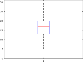
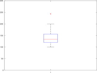
(A) (B)
Figure 3: Boxplots of the bootstrap estimation of the tuning parameter . Similarly, Figure 4 shows the results obtained for the ratio of when . The results for the other marginal are similar. However, since in (5.1), we only display here the ratios of the first marginal.
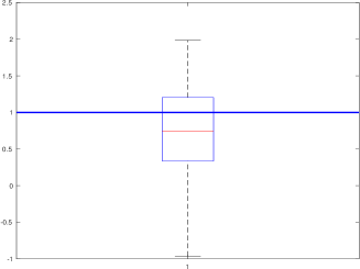
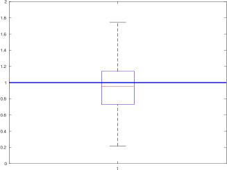
(A) (B)
Figure 4: Boxplots for the ratio . -
2.
Tail index estimation and sequences of normalization : Previous step provides estimations of the marginal tail indexes through moments estimators in (4.1) by using the optimal bootstrap selection of described in Section 4.3. Then, for this simulated data example and without loss of generality, we complete the estimation of by taking the average of the marginal estimations. Finally, the estimations of the sequences of normalization and are given by using (4.2) and (4.3).
-
3.
The scalar function : Note that (3.8) uses the function , which is the stable tail dependence function of the multivariate extreme value distribution . The theoretical tail function for a multivariate distribution is provided by [Nikoloulopoulos et al.(2009)] [Theorem 2.3]. For sake of clarity this result is recalled in Appendix A (see Theorem A.6).
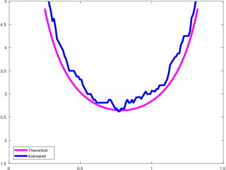
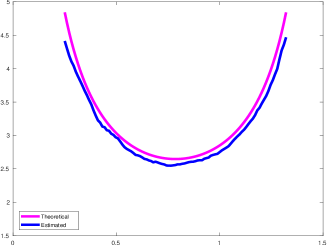
Therefore for any direction , we can calculate and its estimator by using Lemma A.5, Theorem A.6 and Equation (4.4). Figure 5 shows the theoretical curves (in magenta) and the estimated ones (in blue), with the argument described in terms of the angles of its polar parameterization. We can appreciate a good performance of the estimation for both sample sizes. Furthermore, as expected, the larger the sample size, the better the performance of the estimator.
(A) (B)
Figure 5: Theoretical and estimated curves . -
4.
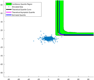
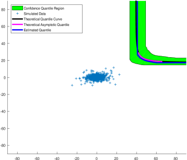
The directional quantile curve : Once the previous steps are completed, both theoretical and estimated results for can be calculated. We use the model to simulate Monte Carlo samples and we apply previous items 1-3 in order to construct point-wise confidence bands. The results are displayed in Figure 6.
(A) (B)
Figure 6: Estimations for . Then, for both sample sizes , Figure 6 shows the theoretical quantiles plotted in black222Theoretical quantiles are the computational iso-curves and iso-surfaces of the multivariate distribution., theoretical asymptotic approximations through the tail function are in magenta, medians point by point of the 100 Monte Carlo estimated curves are in blue and confidence regions from to are shaded in green. We can appreciate the accuracy of the estimations of .
Now, for the FPC direction, we have that theoretical FPC is equal to and the parameters of this directional model are
Thereby, we calculate theoretical and associated estimators by using previous items 1-4. We consider the same sample sizes and Figure 7 presents the results in the same colors as before.
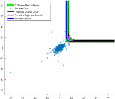
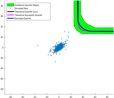
(A) (B)
Figure 7: Estimations for with . Finally, applying the inverse rotation indicated in Equation (4.6), Figure 8 presents the results for . One can appreciate a good performance of our estimators and the improvements on the visualization of extremes, which are more in concordance with the shape of this data-set.
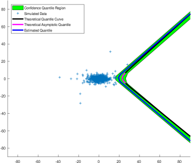
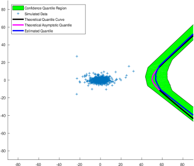
(A) (B)
Figure 8: Estimations for .
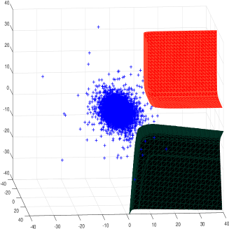
Similar results can be shown for the case presented in (5.1). Firstly, Figure 9 displays the theoretical quantile surfaces at level . The red quantile is performed in the classical direction and the black one is in the direction. These iso-surfaces shown more concordance with the shape of the data when the direction is considered.
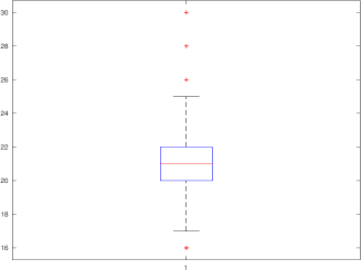
Then, we proceed to illustrate the results through the bootstrap procedure from Figure 10 to Figure 12, but just in the direction, () and without the construction of the point-wise confidence bands. However, in Figure 10 we include Monte Carlo replications to describe the distribution of the tuning parameter selected by bootstrap method. In this trivariate example we consider and .
(A) (B)
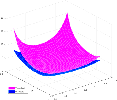
Figure 11 displays the behavior of with described in terms of the angles of its polar parameterization. The estimation is accurate in general, but specially in the central part of the parametric domain of , which is very important to describe properly the behavior of the directional quantile because it represents the region with maximum curvature in the quantile surface. Figure 12 displays the final estimation of .
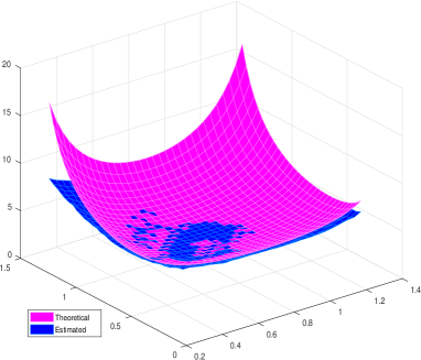
(A) (B)
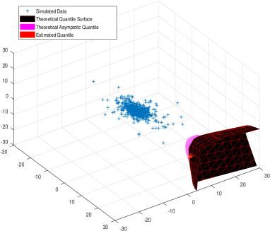
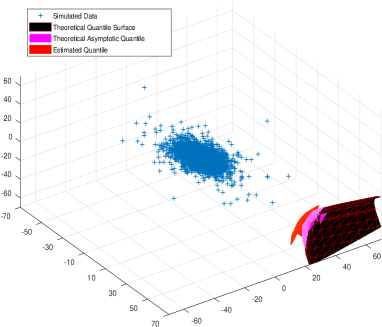
(A) (B)
The visual performance is quite accurate. We introduce in the following a measurement to assess the quality of these results, i.e., the relative error between estimated and asymptotic theoretical quantiles in the point of maximum convexity. By using (3.9) and (4.5), it can be written as
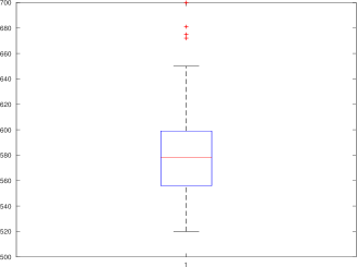
where . Box-plots of for the two considered sample sizes are displayed in Figure 13.
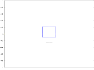
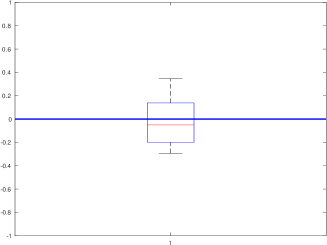
(A) (B)
6 Application to financial real data set
When the object of study is a financial portfolio, the relevance of analysis in the direction of the vector of weights of investment was pointed out in [Torres et al.(2015)]. In this section, the aim is to highlight that the methodology presented in this paper offers an alternative for decision making when investment allocation and particular management criteria are considered. Therefore, we summarize a real case analyzed previously in [He and Einmahl (2017)], describing the main differences between a general analysis of risks through close trimming contours and the specific directional analysis proposed in this paper.
[He and Einmahl (2017)] analyzed the daily market return of a portfolio composed of three international indices from July 2nd, 2001 to June 29th, 2007. The indices are the SP 500 index from USA, the FTSE 100 index from UK and the Nikkei 225 index from Japan. The data contains 1564 observations and it is well-known from the financial literature that stocks returns usually reject the serial independence. Hence, one cannot work with the raw data since the assumption of i.i.d. observations may be inappropriate. [He and Einmahl (2017)] filtered the data to solve this issue. Each time series of market returns was modeled by an exponential GARCH(1,1) and fitted the parameters by maximizing the quasi-likelihood to obtain the filtered returns, also called innovations, which were modeled by a distribution.
As we pointed out in Section 1, methods based on depth and density contours inherently consider the whole set of directions, which provides an overall analysis. However, an analysis considering particular criteria or manager preferences is outside of the aim of those methods. [He and Einmahl (2017)] used the Tukey depth to build out-sample trimming contours for the innovations of these three indices and they suggested to consider the big loss in the US market on February 27th, 2007 as an outlier by considering its innovation far enough based on the high level contour with . Figure 14 displays the results in spherical coordinates to support their claim.
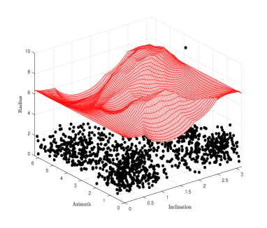
Thus, the region above the surface in Figure 14 accumulates an approximated probability of in its global analysis. However, the directional approach concentrates the level of probability in the set , where can incorporate some manager preferences. Then, the QR oriented orthant in Definition 2.2 can provide an analog rule to identify directional outliers in a similar way as in [He and Einmahl (2017)]. A naive proposal is to consider the fact that the QR oriented orthant in direction divides the space in “disjoint parts” which leads to the value of .
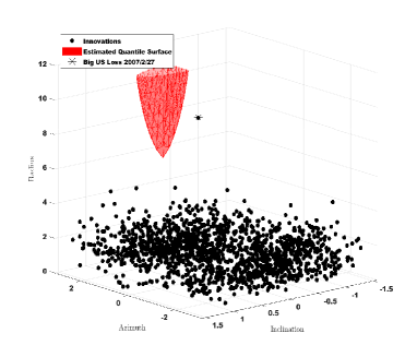
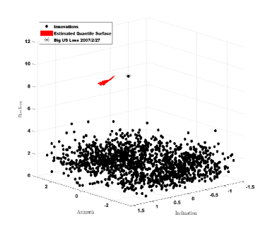
For instance, if the criteria of analysis is the portfolio weights of investment and considering , two examples can be chosen to highlight differences: 1) the naive diversification of the portfolio, i.e., and 2) an investment with large participation in the U.S. market, regular in the U.K. market and small in the Japanese market: . The directional analysis is carried out over the filtered losses, i.e., the negative of the innovations. As in [He and Einmahl (2017)], the filtered losses can be fitted by a multivariate Student distribution, which allows us to perform the directional approach in twofold:
-
1)
A semi-parametric method; that is, the estimation of the parameters of the model for the negative innovations and the calculation of the theoretical directional iso-surfaces for this model by using tools presented in Section 5.
-
2)
Our full non-parametric method presented in Section 4, considering the fact that [He and Einmahl (2017)] previously tested the multivariate regular variation condition on this data-set by the method in [Einmahl and Krajina (2016)].
In Figure 15 we focus in the classical direction . One can see that the big U.S. loss is not identified here as an outlier point because it is not contained in the critical region. This suggests a leverage effect that cannot be underestimated for this particular investment. Conversely, Figure 16 shows that the so called big U.S. loss is indeed above the critical layer for the investment weights . This leads to a similar interpretation of outlier to the one provided by [He and Einmahl (2017)].
(A) Semi-parametric approach (B) Non-parametric approach
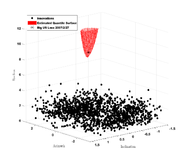
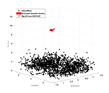
(A) Semi-parametric approach (B) Non-parametric approach
[He and Einmahl (2017)] commented that “Neglecting the joint behaviour can lead to an overestimated diversifiability of risks across international markets and, therefore, underestimation of systematic risk”. In this sense, we add that the directional approach allows to include external information or manager criteria providing a joint local analysis that could lead to different conclusions than those in an overall joint behavior. Furthermore, in [He and Einmahl (2017)] is noted that “an outlier in a high dimensional space is not necessarily an outlier in its subspaces with reduced dimensions”. We also point out that an outlier in one direction is not necessarily an outlier in the other ones.
7 Conclusions
The theory has been extended by the inclusion of the directional framework into it. Also, this paper presented an out-sample characterization of those DMQ , recently introduced in [Torres et al.(2015), Torres et al.(2016)]. Necessary conditions to ensure the estimation of the DMQ at high levels independently of the chosen direction were also presented and the proposed estimator integrates different asymptotic results from the univariate and the multivariate extreme value theory through a parameterization in polar coordinates in .
We introduced an adapted bootstrap-based method to find an optimal solution for the tuning parameter in this multivariate framework, joint to a non-parametric method to complete the estimation of the DMQ. Finally, asymptotic normality of the estimator was derived.
Based on the multivariate distribution, illustrations of the estimation procedure in dimensions 2 and 3 are shown. This family of distributions possesses properties such as heavy tails and closure under rotations, which provides a good example for comparing theoretical and estimated solutions. Finally, a real case study identifying directional outliers in the filtered losses of a financial portfolio is performed. This example suggests that joint local analysis could lead to different conclusions than overall joint behavior. This provides a wider vision to the fact that neglecting the joint behavior can lead to an overestimated diversifiability of risks across international markets.
Future interesting works are to extend the directional framework to the multivariate max-domain of attraction setting, i.e., to relax Assumption A2. Also, to analyze if there exist improvement of estimation by setting independent optimal tuning parameters, for instance, for the estimation of in Equation (4.4). Finally, focusing on applications, it is a task to build a multivariate Value-at-Risk measure in the out-sample framework based on DMQ to analyze risks in different real case scenarios. And also, it is demanding a definition of return period in a general multivariate framework for environmental problems.
Appendix A Auxiliary results and proofs
This section is devoted to the proofs of main results of this paper. Furthermore, different necessary results are introduced below.
Proof of Proposition 3.2. For each Borel set , we have that is a Borel set. Let denote and as the probability measures of and , respectively. For a Borel set , one can write
Therefore, we obtain that the random vector is also multivariate regularly varying with tail index since
Proof of Proposition 3.4. As in the proof of Proposition 3.2, we denote and the probability measures of and , respectively. Then, we get for any relatively compact rectangle that,
Hence,
For the sake of readability, we now introduce the directional multivariate versions of the four lemmas, Lemma 2.1 to Lemma 2.4 in [De Haan and Huang (1995)] without proof. These four lemmas will be useful to prove Proposition 4.1 below.
Lemma A.1.
If has continuous first-order derivatives , then
converges to
Lemma A.2.
Lemma A.3.
Under the conditions of Proposition 4.1,
Lemma A.4.
Let . Then, under the conditions of Proposition 4.1,
The proofs of these lemmas work in a similar way as in [De Haan and Huang (1995)] considering the arrangements due to the directional multivariate framework, then they are omitted here. Now, by using Lemmas A.1-A.4, one can prove the main Proposition 4.1.
Proof of Proposition 4.1. Lemma A.1 proves asymptotic convergence of the standardized difference . This implies asymptotic normality of the standardized difference in Lemma A.2.
Also, Lemma A.3 proves the convergence to zero of the standardized difference , which helps to prove Lemma A.4 where the convergence to zero of the standardized difference is given. Then, by using the asymptotic normality of the standardized difference between the approximation and the estimation in Lemma A.2 and the convergence to zero of the standardized difference between the true elements and its approximations in Lemma A.4, the result in Proposition 4.1 is achieved.
We recall below an useful result for elliptical distribution (see Lemma 3.1 in [Hult and Lindskog (2002)]).
Lemma A.5.
If has an elliptical distribution and decomposition given by
where is a random variable independent from the random vector , which is uniformly distributed in the unit circle of dimension , a location parameter and a matrix indicating scale. Then, for any orthogonal matrix , has an elliptical distribution with associated decomposition given by
Moreover, its marginals are the associated univariate elliptical distributions with parameters of location and scale given by and .
Now we summarize the result from [Nikoloulopoulos et al.(2009)], where the theoretical stable tail dependence function for a multivariate distribution is obtained. The interested reader is also referred to [Opitz (2013)].
Theorem A.6 ([Nikoloulopoulos et al.(2009)], Theorem 2.3).
The theoretical tail function of , a dimensional distribution with d.f. , location parameter and scale parameter , is given by,
where are the correlations between the components , is a distribution in dimension (removing the component), with d.f. , location parameter and scale parameter given by,
where , for .
Acknowledgments
This research was partially supported by a Spanish Ministry of Economy and Competitiveness grant ECO2015-66593-P, the French project LEFE-MANU MULTIRISK and by Consejería de Educación de la Junta de Castilla y León and FEDER funds (ref. VA005P17).
References
- [Basrak et al.(2002)] Basrak B., Davis R., and Mikosch T. (2002). Regular variation of GARCH processes, Stochastic Processes and Their Applications, 99, 95-115.
- [Belzunce et al.(2007)] Belzunce F., Castaño A., Olvera-Cervantes A. and Suárez-Llorens A. (2007). Quantile curves and dependence structure for bivariate distributions. Computational Statistical Data Analysis, 51, 5112-5129.
- [Binois et al.(2015)] Binois M., Rullieèrec D. and Roustant O. (2015). On the estimation of Pareto fronts from the point of view of copula theory. Information Sciences, 324, 270-285.
- [Cai et al.(2011)] Cai J., Einmahl J., and de Haan L. (2011). Estimation of extreme risk regions under multivariate regular variation. Annals of Statistics, 39(3), 1803-1826.
- [Cai et al.(2015)] Cai J., Einmahl J., de Haan L., and Zhou C. (2015). Estimation of the marginal expected shortfall: the mean when a related variable is extreme. Journals of the Royal Statistical Society. Series B. Statistical Methodology, 77(2), 417-442.
- [Chatterjee and Chatterjee (1990)] Chatterjee S. and Chatterjee S. (1990). A note on finding extreme points in multivariate space. Computational Statistics Data Analysis, 10(1), 87-92.
- [Chaudhuri (1996)] Chaudhuri P. (1996). On a geometric notion of quantiles for multivariate data. Journal of the American Statistical Association, 91, 862-872.
- [Chebana and Ouarda (2009)] Chebana F. and Ouarda T. (2009). Index flood-based multivariate regional frequency analysis. Water Resour. Res., 45, W10435.
- [Chebana and Ouarda (2011)] Chebana F. and Ouarda T. (2011). Multivariate quantiles in hydrological frecuency analysis. Envirometrics, 22, 63-78.
- [Cousin and Di Bernardino (2013)] Cousin A. and Di Bernardino E. (2013). On multivariate extensions of Value-at-Risk. Journal of Multivariate Analysis, 119, 32-46.
- [Danielsson et al.(2001)] Danielsson J., de Haan L. and De Vries C. (2001). Using a Bootstrap Method to Choose the Sample Fraction in Tail Index Estimation, Journal of Multivariate Analysis, 76, 226-248.
- [De Haan and Ferreira (2006)] de Haan L. and Ferreira A. (2006). Extreme Value Theory, An Introduction. Springer, New York.
- [De Haan and Huang (1995)] de Haan L., and Huang X. (1995). Large Quantile Estimation in a Multivariate Setting. Journal of Multivariate Analysis, 53, 247-263.
- [De Haan and Resnick (1993)] de Haan L. and Resnick S. (1993). Estimating the Limit Distribution of Multivariate Extremes. Commun. Statist. - Stochastic Models, 9, 275-309.
- [Dekkers et al.(1989)] Dekkers A. Einmahl J. and de Haan L. (1989). A moment estimator for the index of an extreme-value distribution. Annals of Statistics, 17, 1833-1855.
- [Di Bernardino et al.(2011)] Di Bernardino E., Laloe T., Maume-Deschamps V. and Prieur C. (2011). Plug-in estimation of level sets in a non-compact setting with applications in multivariate risk theory. ESAIM: Probability and Statistics, 17, 236-256.
- [Di Bernardino et al.(2015)] Di Bernardino E., Fernández-Ponce J., Palacios-Rodríguez F., Rodíguez-Griñolo M. (2015). On multivariate extensions of the conditional Value-at-Risk measure. Insurance: Mathematics and Statistics, 61, 1-16.
- [Di Bernardino and Palacios-Rodríguez (2016)] Di Bernardino E. and Palacios-Rodríguez, F. (2016). Estimation of extreme quantiles conditioning on multivariate critical layers. Environmetrics, 27(3), 158-168.
- [Draisma et al.(1999)] Draisma G., de Haan L., Peng L. and Pereira T. (1999). A bootstrap-based method to achieve optimality in estimating the extreme-value index. Extremes 2, 367-404.
- [Driver (2003)] Driver B. (2003). Analysis Tools with Applications. Springer, Berlin.
- [Durante and Salvadori (2010)] Durante F. and Salvadori G. (2010). On the construction of multivariate extreme value models via copulas. Envirometrics, 21, 143-161.
- [Einmahl et al.(2013)] Einmahl J., de Haan L. and Krajina A. (2013). Estimating extreme bivariate quantile regions. Extremes, 16 (2), 121-145.
- [Einmahl and Krajina (2016)] Einmahl J. and Krajina A. (2016). Empirical likelihood based testing for multivariate regular variation. Tilburg University, Tilburg.
- [Embrechts and Puccetti (2006)] Embrechts P. and Puccetti G. (2006). Bounds for functions of multivariate risks. Journal of Multivariate Analysis, 97, 526-547.
- [Ferreira et al.(2003)] Ferreira A., de Haan L., Peng L. (2003). On optimising the estimation of high quantiles of a probability distribution. Statistics 37(5), 401-434.
- [Fraiman and Pateiro-López (2012)] Fraiman R. and Pateiro-López B. (2012). Quantiles for finite and infinite dimensional data. Rutcor Research Report 25.
- [Fernández-Ponce and Suárez-Llorens (2002)] Fernández-Ponce J. and Suárez-Llorens A. (2002). Central regions for bivariate distributions. Austrian Journal of Statistics, 31, 141-156.
- [Girard and Stupfler (2015)] Girard S. and Stupfler G. (2015). Extreme geometric quantiles in a multivariate regular variation framework. Extremes, 18, 629-663.
- [Gupta and Manohar (2005)] Gupta S. and Manohar C. (2005). Multivariate extreme value distributions for random vibration applications. Journal of engineering mechanics, 131(7), 712-720.
- [Hallin et al.(2010)] Hallin M., Paindaveine D. and Šiman M. (2010). Multivariate quantiles and multiple-output regression quantiles: from optimization to halfspace depth. Annals of Statistics, 38, 635-669.
- [He and Einmahl (2017)] He, Y. and Einmahl, J. H. J. (2017). Estimation of extreme depth-based quantile regions. Journals of the Royal Statistical Society, Series B, Statistical Methodology, 79, 449-461.
- [Horn and Johnson (2013)] Horn R. and Johnson C. (2013). Matrix Analysis. Cambridge University Press, 2nd Ed.
- [Hua and Joe (2011)] Hua, L., and H. Joe. (2011). Second Order Regular Variation and Conditional Tail Expectation of Multiple Risks. Insurance: Mathematics and Economics 49, 537-546.
- [Hult and Lindskog (2002)] Hult H. and Lindskog F. (2002). Multivariate extremes, aggregation and dependence in elliptical distributions. Advances in Applied Probability, 34, 587-608.
- [Jessen and Mikosh (2006)] Jessen A. and Mikosh T. (2006). Regularly varying functions. Publications de l’institute mathematique, 79.
- [Kong and Mizera (2012)] Kong L. and Mizera I. (2012). Quantile tomography: Using quantiles with multivariate data. Statistica Sinica, 22(4), 1589-1610.
- [Laniado et al.(2012)] Laniado H., Lillo R., Pellerey F. and Romo J. (2012). Portfolio selection through an extremality stochastic order. Insurance: Mathematics and Economics, 51, 1-9.
- [Mikosch (2003)] Mikosch T. (2003). Modeling dependence and tails of financial time series. In: Finkenstädt, B., Rootzén, H. (eds.) Extreme Values in Finance, Telecommunications, and the Environment, 187-286, Chapman Hall, Boca Raton.
- [Mukhopadhyay and Chatterjee (2011)] Mukhopadhyay N. and Chatterjee S. (2011). High dimensional data analysis using multivariate generalized spatial quantiles. Journal of Multivariate Analysis, 102 (4), 768-780.
- [Nikoloulopoulos et al.(2009)] Nikoloulopoulos A., Joe H. and Li H. (2009). Extreme value properties of multivariate t copulas. Extremes, 12, 129-148.
- [Opitz (2013)] Opitz T. (2013). Extremal processes: Elliptical domain of attraction and a spectral representation, Journal of Multivariate Analysis, 122, 409-413.
- [Qi (2008)] Qi Y., Bootstrap and empirical likelihood methods in extremes, Extremes 11, 81-97, (2008).
- [Resnick (1987)] Resnick S. (1987). Extreme values, regular variation and point process. Springer-Verlag.
- [Resnick (2002)] Resnick, S. (2002). Hidden regular variation, second order regular variation, and asymptotic independence. Extremes, 5, 303-336.
- [Resnick (2007)] Resnick S. (2004). Heavy-tail Phenomena: Probabilistic and Statistical Modeling. Springer, New York, (2007).
- [Salvadori (2004)] Salvadori, G., Bivariate return periods via 2-copulas. Statist. Methodol., 1, 129-144.
- [Salvadori et al.(2011)] Salvadori G., De Michele C. and Durante F. (2011). On the return period and design in a multivariate framework. Hydrol. Earth Syst. Sci., 15, 3293-3305.
- [Serfling (2002)] Serfling R. (2002). Generalized quantile processes based on multivariate depth function, with applications in nonparametric multivariate analysis. Journal of Multivariate Analysis, 83, 232-247.
- [Shiau (2003)] Shiau J. (2003). Return period of bivariate distributed extreme hydrological events, Stochastic Environmental Research and Risk Assessment, 17, 42-57.
- [Torres et al.(2015)] Torres R. (2015). Lillo R. and Laniado H., A Directional Multivariate Value at Risk. Insurance: Mathematics and Economics, 65, 111-123.
- [Torres et al.(2016)] Torres R. (2017). De Michele C., Laniado H. and Lillo R., Directional Multivariate Extremes in Environmental Phenomena. Environmetrics, 28 (2), e2428.
- [Rachev et al.(2013)] Rachev, S. (2013). Klebanov, L., Stoyanov, S., and Fabozzi, F. The methods of distances in the theory of probability and statistics. Springer Series in Probability Theory and Stochastic Processes. Springer, New York.