Nonparametric Dynamic State Space Modeling of Observed Circular Time Series with Circular Latent States: A Bayesian Perspective

Abstract

Circular time series has received relatively little attention in statistics and modeling complex circular time series using the state space approach is non-existent in the literature. In this article we introduce a flexible Bayesian nonparametric approach to state space modeling of observed circular time series where even the latent states are circular random variables. Crucially, we assume that the forms of the observational and evolutionary functions, both of which are circular in nature, are unknown and time-varying. We model these unknown circular functions by appropriate wrapped Gaussian processes having desirable properties.

We develop an effective Markov chain Monte Carlo strategy for implementing our Bayesian model by judiciously combining Gibbs sampling and Metropolis-Hastings methods. Validation of our ideas with a simulation study and two real bivariate circular time series data sets, where we assume one of the variables to be unobserved, revealed very encouraging performance of our model and methods.

We finally analyse a data consisting of directions of whale migration, considering the unobserved ocean current direction as the latent circular process of interest. The results that we obtain are encouraging, and the posterior predictive distribution of the observed process correctly predicts the observed whale movement.
Keywords: Circular time series; Latent circular process; Look-up table; Markov Chain Monte Carlo; State-space model; Wrapped Gaussian process.

1 Introduction

In contrast with the traditional time series where the variables take values on the real line, circular time series with angular variables have received much less attention in the statistical literature. Some of the relatively scarce undertakings on circular time series, all in the classical statistical framework, are Breckling (1989), Fisher and Lee (1994), Holzmann et al. (2006), Hughes (2007) and Di Marzio et al. (2012). The classical approach, however, is limited to models with relatively simple dependence structures, such as the $p$-th order Markov dependence, to enable inference. Far more flexible and realistic models can be accommodated within the Bayesian paradigm without any compromise; the inference can be carried out arbitrarily accurately using powerful Markov chain Monte Carlo (MCMC) methods. In this article, we propose and develop a novel and highly flexible approach to modeling circular time series using a Bayesian nonparametric state space approach, and an effective MCMC methodology for Bayesian inference.

Indeed, versatility of state space structures in modeling complex time series is well-appreciated in various scientific disciplines such as statistics, engineering, economics, biology, ecology, finance, and most of the existing time series models admit the state space representation. Notably, state space models consist of an observational equation for the observed part of the time series and an evolutionary equation that accounts for the latent, unobserved process that is presumed to affect the observed process. In this work, we shall concern ourselves with Bayesian state space modeling of complex circular time series data, where the latent process is also circular in nature, and where the observational and evolutionary functions are time-varying, but unknown. We model both the unknown functions nonparametrically using appropriate wrapped Gaussian process priors developed by Mazumder and Bhattacharya (2016a). For our state space model, the circular observations are conditionally independent given the latent states and the observational function, and the latent states have the Markov property conditionally on the evolutionary function. Unconditionally, however, the latent circular states are realizations of a complex, intractable stochastic process possessing a complex, intractable dependence structure in a way that all the latent states depend upon each other. The observed circular process is also intractable unconditionally, with a dependence structure that makes all the observational variables interdependent. However, the attractive properties of the wrapped Gaussian process prior ensure that the dependence structure, although complex, is very reasonable. Thus, our Bayesian state space modeling approach frees the circular time series paradigm of the limitations of the classical approach, while the MCMC procedure we propose, takes care of the inference part.

It is worth noting that Mazumder and Bhattacharya (2016a) developed a Bayesian nonparametric state space approach to modeling observed linear time series, assuming circular latent process. The obvious difference of our current work with theirs is that in our case, even the observed time series is circular. This circular extension of the observed process, however, is not insignificant, and throws much difficult challenges compared to the approach of Mazumder and Bhattacharya (2016a). In particular, because of our Gaussian process approach, the joint distribution of the observed data conditional on the latent states and the other parameters, is a product of wrapped normal distributions, for which closed forms are not available, and as many discrete auxiliary variables as the data size are needed to be introduced to express the likelihood conditional on the auxiliary variables. To make things harder, these wrapped normal distributions, even conditionally on the auxiliary variables, involve the unknown observational function in a way that it can not be integrated out as in Mazumder and Bhattacharya (2016a). Indeed, thanks to the linear nature of the observed process, Mazumder and Bhattacharya (2016a) could marginalize over the unknown observational function to arrive at a multivariate normal distribution of the observed data conditionally on the latent states and other parameters.

Combination of our involved conditional distribution of the observed data with the heavily involved form of the joint distribution of the state variables yields a structure that is way beyond the scope of Mazumder and Bhattacharya (2016a). It is thus clear that in comparison with Mazumder and Bhattacharya (2016a), a substantially different and involved MCMC method is also required for the implementation of our approach.

Once we build the necessary Bayesian nonparametric model and methods, we evaluate them on a simulated data generated from a state space model with specific circular observational and circular evolutionary equations, but fitted with our proposed model and methods. We also consider two real data sets for validation of our ideas. In one case, wind directions at $6.00$ am and $12.00$ pm on each of 21 days, are recorded. Pretending that the wind directions at $6.00$ am are unobserved, we obtain the posteriors of these circular latent states and compare it with the actual observed values. The second data set for our validation purpose consists of spawning time of a particular fish and the low tide times, both measured on the 24-hour clock, for 86 days. In this case, we assume that the low tide times are unobserved, and fit our Bayesian model, viewing the times as circular variables. In all the three cases, we obtained excellent predictions of the latent circular states and excellent forecasts of both latent and observed states.

We then apply our ideas to a real data set consisting of only the directions associated with movements of a whale in course of its migration. The directions of ocean current, which are presumed to influence the movements of the whale, are not observed, and hence, we consider them to be the latent circular states of our interest. Our Bayesian model and methods yielded quite sensible results on the latent states and correct prediction of the whale movement.

The rest of this article is structured as follows. In Section 2 we introduce our Bayesian state space model with circular observed data and circular latent states, discussing our wrapped Gaussian process prior and explicitly providing the form of the Bayesian hierarchical model, and the forms of the priors on the parameters. In Section 3 we briefly discuss the main technical issues distinguishing our MCMC method with that of Mazumder and Bhattacharya (2016a), showing that our present MCMC methodology is far more involved. The details of our MCMC procedure are provided in the supplement Mazumder and Bhattacharya (2016b). We then validate our model and methods with a simulation study in Section 4 and two real data sets on pairs of wind directions and spawning/low tide times in Section 5. We apply our ideas to the whale data in Section 6, obtaining the posteriors of the ocean current directions and forecasting whale movement. Finally, we summarize our work and provide concluding remarks in Section 7.

2 Dynamic state space model with circular latent and observed states

Our proposed state space model is as follows: For $t=1,2,\ldots T$,

$$y_{t} =\left\{f(t,x_{t})+\epsilon_{t}\right\}~{}[2\pi],~{}~{}\epsilon_{t}\sim N(0,\sigma^{2}_{\mbox{\scriptsize{$\epsilon$}}}),$$ (1)

$$x_{t} =\left\{g(t,x_{t-1})+\eta_{t}\right\}~{}[2\pi],~{}~{}\eta_{t}\sim N(0,\sigma^{2}_{\mbox{\scriptsize{$\eta$}}}),$$ (2)

where $\{y_{t};~{}t=1,\ldots,T\}$ is the observed circular time series; $\{x_{t};~{}t=0,1,\ldots,T\}$ are the latent circular states; $f(\cdot,\cdot)$ and $g(\cdot,\cdot)$ are the unknown evolutionary functions with values on the circular manifold. In equations (1) and (2), $[2\pi]$ stands for the $\mbox{mod}~{}2\pi$ operation. Note that

$$\left\{f(t,x_{t})+\epsilon_{t}\right\}~{}[2\pi] =\left\{f^{*}(t,x_{t})+\epsilon_{t}\right\}~{}[2\pi]$$ (3)

and

$$\left\{g(t,x_{t-1})+\eta_{t}\right\}~{}[2\pi] =\left\{g^{*}(t,x_{t-1})+\eta_{t}\right\}~{}[2\pi],$$ (4)

where $f^{*}$ and $g^{*}$ are the linear counterparts of $f$ and $g$, that is, $f^{*}(t,x_{t})$ is the linear random variable such that $f^{*}(t,x_{t})~{}[2\pi]=f(t,x_{t})$ and similarly, $g^{*}(t,x_{t-1})~{}[2\pi]=g(t,x_{t-1})$. For convenience, we shall frequently use the representations (3) and (4). For more details on such a representation the reader is referred to Mazumder and Bhattacharya (2016a). Indeed, to derive the distributions of $y_{t}$ and $x_{t}$, we shall first obtain the distributions of the linear random variables $f^{*}(t,x_{t})+\epsilon_{t}$ and $g^{*}(t,x_{t-1})+\eta_{t}$ and then apply the $\mbox{mod}~{}2\pi$ operation to these variables to derive the distribution of the circular variables $y_{t}$ and $x_{t}$.

Note that both the observational and evolutionary functions have the linear argument $t$ and the angular argument $x$. The linear argument guarantees that the functions are time-varying, that is, the functions are allowed to freely evolve with time.

2.1 Wrapped Gaussian process representations of the observational and evolutionary functions

We now provide a brief discussion on modeling the unknown circular functions $f$ and $g$. Mazumder and Bhattacharya (2016a) have constructed a wrapped Gaussian process by convolving a suitable kernel with standard Wiener process as a function of time and directions. The created wrapped Gaussian process has the desirable properties; for example, the covariance becomes 0 whenever the difference between the angles becomes $\pi/2$, implying orthogonality of the directions, irrespective of the value of the time difference. Similarly, as the time difference goes to $\infty$, the covariance converges to 0. Moreover, the desired continuity and smoothness properties do hold for the constructed Gaussian process (the proofs are provided in the supplement of Mazumder and Bhattacharya (2016a)). While constructing such a wrapped Gaussian process the basic idea was to first construct a Gaussian process as a function of time and angle and then apply the mod $2\pi$ operation. Here also, to model $f$ and $g$, we first model $f^{*}$ and $g^{*}$, the linear parts of $f$ and $g$, using the Gaussian process, created in Mazumder and Bhattacharya (2016a). The mean functions of $f^{*}$ and $g^{*}$ are of the forms $\mu_{f}(\cdot,\cdot)$ = $\mbox{\boldmath{$h$}}(\cdot,\cdot)^{\prime}\mbox{\boldmath{$\beta$}}_{f}$ and $\mu_{g}(\cdot,\cdot)$ = $\mbox{\boldmath{$h$}}(\cdot,\cdot)^{\prime}\mbox{\boldmath{$\beta$}}_{g}$, where $\mbox{\boldmath{$h$}}(t,z)$ = $(1,t,\cos(z),\sin(z))^{\prime}$; here $z$ is an angular quantity and $\mbox{\boldmath{$\beta$}}_{f}$, $\mbox{\boldmath{$\beta$}}_{g}$ are parameters in $\mathbb{R}^{4}$. For any fixed $(t_{1},z_{1})$ and $(t_{2},z_{2})$, where $t_{1},t_{2}$ are linear quantities and $z_{1},z_{2}$ are angular quantities, the covariance structures are given by $c_{f}((t_{1},z_{1}),(t_{2},z_{2}))$ = $\exp\{-\sigma_{f}^{4}(t_{1}-t_{2})^{2}\}\cos(|z_{1}-z_{2}|)$ and $c_{g}((t_{1},z_{1}),(t_{2},z_{2}))$ = $\exp\{-\sigma_{g}^{4}(t_{1}-t_{2})^{2}\}\cos(|z_{1}-z_{2}|)$, where $\sigma_{f}$ and $\sigma_{g}$ are positive, real valued parameters. For details, see Mazumder and Bhattacharya (2016a). After modeling $f^{*}$ and $g^{*}$ by the aforementioned Gaussian process, we derive the wrapped Gaussian distribution of $f(\cdot,\cdot)+\epsilon_{t}$ and $g(\cdot,\cdot)+\eta_{t}$ using the mod $2\pi$ operation on the distributions of $f^{*}(\cdot,\cdot)+\epsilon_{t}$ and $g^{*}(\cdot,\cdot)+\eta_{t}$, respectively.

2.2 Bayesian hierarchical structure of our proposed model

Our modeling approach can be described succinctly by the following hierarchical Bayesian representation:

$$[y_{t}|f,\mbox{\boldmath{$\theta$}}_{f},x_{t}] \sim N\left(f^{*}(t,x_{t}),\sigma^{2}_{\epsilon}\right)~{}[2\pi];~{}t=1,\ldots,T,$$ (5)

$$[x_{t}|g,\mbox{\boldmath{$\theta$}}_{g},x_{t-1}] \sim N\left(g^{*}(t,x_{t-1}),\sigma^{2}_{\eta}\right)[2\pi];~{}t=1,\ldots,T,$$ (6)

$$[f(\cdot,\cdot)|\mbox{\boldmath{$\theta$}}_{f}] \sim GP\left(\mbox{\boldmath{$h$}}(\cdot,\cdot)^{\prime}\mbox{\boldmath{$\beta$}}_{f},\sigma^{2}_{f}c_{f}(\cdot,\cdot)\right)~{}[2\pi],$$ (7)

$$[g(\cdot,\cdot)|\mbox{\boldmath{$\theta$}}_{g}] \sim GP\left(\mbox{\boldmath{$h$}}(\cdot,\cdot)^{\prime}\mbox{\boldmath{$\beta$}}_{g},\sigma^{2}_{g}c_{g}(\cdot,\cdot)\right)[2\pi],$$ (8)

$$[\mbox{\boldmath{$\beta$}}_{f},\sigma^{2}_{f},\mbox{\boldmath{$\beta$}}_{g},\sigma^{2}_{g},\sigma^{2}_{\epsilon},\sigma^{2}_{\eta}] =[\mbox{\boldmath{$\beta$}}_{f},\sigma^{2}_{f}][\mbox{\boldmath{$\beta$}}_{g},\sigma^{2}_{g}][\sigma^{2}_{\epsilon},\sigma^{2}_{\eta}],$$ (9)

where $\mbox{\boldmath{$\theta$}}_{f}=(\mbox{\boldmath{$\beta$}}_{f},\sigma_{f},\sigma_{\epsilon})^{\prime}$ and $\mbox{\boldmath{$\theta$}}_{g}=(\mbox{\boldmath{$\beta$}}_{g},\sigma_{g},\sigma_{\eta})^{\prime}.$ In the above, GP stands for “Gaussian Process”.

For obtaining the joint distribution of the latent circular state variables, we utilize the “look-up” table approach (see Bhattacharya (2007)) along the same line as Mazumder and Bhattacharya (2016a). The idea and the complete details of the look-up table approach in the context of circular latent variable is discussed in Mazumder and Bhattacharya (2016a), and thereby we skip the details in this current article. In the next section we provide the forms of the prior distributions of the parameters associated with the above hierarchical structure.

2.3 Prior specifications

Our prior distributions have the following forms.

$$[x_{0}] \sim\mbox{von-Mises}(\mu_{0},\sigma_{0}^{2});$$ (10)

$$[\sigma^{2}_{\mbox{\scriptsize$\epsilon$}}] \propto(\sigma^{2}_{\mbox{\scriptsize$\epsilon$}})^{\left(-\frac{\alpha_{\mbox{\tiny$\epsilon$}}+2}{2}\right)}\mbox{ exp }\left\{-\frac{\gamma_{\mbox{\tiny$\epsilon$}}}{2\sigma^{2}_{\mbox{\scriptsize$\epsilon$}}}\right\};~{}~{}\alpha_{\mbox{\tiny$\epsilon$}},\,\gamma_{\mbox{\tiny$\epsilon$}}>0$$ (11)

$$[\sigma^{2}_{\mbox{\scriptsize$\eta$}}] \propto(\sigma^{2}_{\mbox{\scriptsize$\eta$}})^{\left(-\frac{\alpha_{\mbox{\tiny$\eta$}}+2}{2}\right)}\mbox{ exp }\left\{-\frac{\gamma_{\mbox{\tiny$\eta$}}}{2\sigma^{2}_{\mbox{\scriptsize$\eta$}}}\right\};~{}~{}\alpha_{\mbox{\tiny$\eta$}},\,\gamma_{\mbox{\tiny$\eta$}}>0$$ (12)

$$[\sigma^{2}_{g}] \propto(\sigma^{2}_{g})^{\left(-\frac{\alpha_{\mbox{\tiny$g$}}+2}{2}\right)}\mbox{ exp }\left\{-\frac{\gamma_{\mbox{\tiny$g$}}}{2\sigma^{2}_{g}}\right\};~{}~{}\alpha_{\mbox{\tiny$g$}},\,\gamma_{\mbox{\tiny$g$}}>0$$ (13)

$$[\sigma^{2}_{f}] \propto(\sigma^{2}_{f})^{\left(-\frac{\alpha_{\mbox{\tiny$f$}}+2}{2}\right)}\mbox{ exp }\left\{-\frac{\gamma_{\mbox{\tiny$f$}}}{2\sigma^{2}_{f}}\right\};~{}~{}\alpha_{\mbox{\tiny$f$}},\,\gamma_{\mbox{\tiny$f$}}>0$$ (14)

$$[\mbox{\boldmath{$\beta$}}_{f}] \sim N_{4}(\mbox{\boldmath{$\beta$}}_{f,0},\mbox{\boldmath{$\Sigma$}}_{\beta_{f,0}});$$ (15)

$$[\mbox{\boldmath{$\beta$}}_{g}] \sim N_{4}(\mbox{\boldmath{$\beta$}}_{g,0},\mbox{\boldmath{$\Sigma$}}_{\beta_{g,0}}).$$ (16)

Here, by $N_{4}(\cdot,\cdot)$, we mean the 4 variate normal distribution. We discuss the choice of prior parameters in Sections 4, 5 and 6, in the contexts of applications to simulated and real data sets.

3 MCMC-based inference

The aim of our MCMC-based inference is to address the problem of forecasting $y_{T+1}$ and to learn about the latent circular states, given the observed data set $\mbox{\boldmath{$D$}}_{T}=(y_{1},\ldots,y_{T})^{\prime}$. Unlike Mazumder and Bhattacharya (2016a) here $y_{t}$ is circular and hence dealing with the conditional distribution of $y_{T+1}$ given the data $\mbox{\boldmath{$D$}}_{T}$ is rendered far more difficult. As already remarked in Section 1, the distribution of the observed variables is circular normal, and does not admit any closed form expression. To deal with such a situation one needs to bring in the auxiliary variables $N_{t}$ = $\langle y_{t}^{*}/2\pi\rangle$, where $y_{t}^{*}$ is the linear part of the circular variable $y_{t}$ and $\langle u\rangle$ denotes the largest integer not exceeding $u$. The wrapped random variable $N_{t}$ can take values in the set $\mathbb{Z}$, where $\mathbb{Z}$ denotes the set of the integers. For details on wrapped variable in the context of circular data, see, for example, Ravindran and Ghosh (2011); see also Mazumder and Bhattacharya (2016a). However, even conditionally on the auxiliary variables, $f^{*}$ can not be marginalized out of the model to simplify the proceedings, so that our MCMC method must include simulation of $f^{*}$, in addition to the auxiliary variables. In contrast, Mazumder and Bhattacharya (2016a) was able to work with a much simpler form thanks to joint conditional normality of their linear observed data, which also enabled them to integrate out the unknown observational function, further simplifying their proceedings.

In our case, the posterior distribution of $y_{T+1}$ given $\mbox{\boldmath{$D$}}_{T}$ admits the following form after introducing the auxiliary variables $N_{1},\ldots,N_{T}$:

$$[y_{T+1}|\mbox{\boldmath{$D$}}_{T}]$$

$$=\sum_{N_{1},\ldots,N_{T}}\int\left[y_{T+1}|\mbox{\boldmath{$D$}}_{T},f^{*}(1,x_{1}),\ldots,f^{*}(T+1,x_{T+1}),N_{1},\ldots N_{T},x_{0},\ldots,x_{T+1},\mbox{\boldmath{$\beta$}}_{f},\mbox{\boldmath{$\beta$}}_{g},\sigma_{f},\right.$$

$$\quad\left.\sigma_{g},\sigma_{\epsilon},\sigma_{\eta}\right][f^{*}(1,x_{1}),\ldots,f^{*}(T+1,x_{T+1}),N_{1},\ldots N_{T},x_{0},\ldots,x_{T+1},\mbox{\boldmath{$\beta$}}_{f},\mbox{\boldmath{$\beta$}}_{g},\sigma_{f},\sigma_{g},\sigma_{\epsilon},\sigma_{\eta}|\mbox{\boldmath{$D$}}_{T}]$$

$$\quad df^{*}(1,x_{1})\ldots df^{*}(T+1,x_{T+1})dx_{0}\ldots dx_{T+1}d\mbox{\boldmath{$\beta$}}_{f}d\mbox{\boldmath{$\beta$}}_{g}d\sigma_{f}d\sigma_{g}d\sigma_{\epsilon}d\sigma_{\eta}.$$ (17)

Therefore, once we have a sample from the joint posterior $[f^{*}(1,x_{1}),\ldots,f^{*}(T+1,x_{T+1}),N_{1},\ldots,N_{T},x_{0},\ldots,\\ x_{T+1},\mbox{\boldmath{$\beta$}}_{f},\mbox{\boldmath{$\beta$}}_{g},\sigma_{f},\sigma_{g},\sigma_{\epsilon},\sigma_{\eta}|\mbox{\boldmath{$D$}}_{T}]$, we can generate an observation from $[y_{T+1}|\mbox{\boldmath{$D$}}_{T}]$ by simply generating an observation from $[y_{T+1}|\mbox{\boldmath{$D$}}_{T},f^{*}(1,x_{1}),\ldots,f^{*}(T+1,x_{T+1}),N_{1},\ldots N_{T},x_{0},\ldots,x_{T+1},\mbox{\boldmath{$\beta$}}_{f},\mbox{\boldmath{$\beta$}}_{g},\sigma_{f},\sigma_{g},\sigma_{\epsilon},\sigma_{\eta}]$. Further, we note that given a sample from $[f^{*}(1,x_{1}),\ldots,f^{*}(T+1,x_{T+1}),N_{1},\ldots N_{T},x_{0},\ldots,x_{T+1},\mbox{\boldmath{$\beta$}}_{f},\mbox{\boldmath{$\beta$}}_{g},\sigma_{f},\sigma_{g},\\ \sigma_{\epsilon},\sigma_{\eta}|\mbox{\boldmath{$D$}}_{T}]$, $y_{T+1}$ has a wrapped normal distribution with parameter $f^{*}(T+1,x_{T+1})\mbox{ and }\sigma^{2}_{\epsilon}$, because

$$[y_{T+1}|\mbox{\boldmath{$D$}}_{T},f^{*}(1,x_{1}),\ldots,f^{*}(T+1,x_{T+1}),N_{1},\ldots N_{T},x_{0},\ldots,x_{T+1},\mbox{\boldmath{$\beta$}}_{f},\mbox{\boldmath{$\beta$}}_{g},\sigma_{f},\sigma_{g},\sigma_{\epsilon},\sigma_{\eta}]$$

$$= [y_{T+1}|f^{*}(T+1,x_{T+1}),\sigma_{\epsilon},x_{T+1}].$$

Therefore, we need to obtain a sample from $[f^{*}(1,x_{1}),\ldots,f^{*}(T+1,x_{T+1}),N_{1},\ldots N_{T},x_{0},\ldots,x_{T+1},\\ \mbox{\boldmath{$\beta$}}_{f},\mbox{\boldmath{$\beta$}}_{g},\sigma_{f},\sigma_{g},\sigma_{\epsilon},\sigma_{\eta}|\mbox{\boldmath{$D$}}_{T}]$. Define $\mbox{\boldmath{$f$}}^{*}$ = $(f^{*}(1,x_{1}),\ldots,f^{*}(T+1,x_{T+1}))^{\prime}$ = $(\mbox{\boldmath{$f$}}_{\mbox{\scriptsize$D_{T}$}}^{*},f^{*}(T+1,x_{T+1}))^{\prime}$. Note that given $(x_{1},\ldots,x_{T+1})^{\prime},\mbox{\boldmath{$\beta$}}_{f},\mbox{ and }\sigma_{f}$, $\mbox{\boldmath{$f$}}^{*}$ follows a $(T+1)$-variate normal distribution with mean $E[\mbox{\boldmath{$f$}}^{*}|(x_{1},\ldots,\\ x_{T+1})^{\prime},\mbox{\boldmath{$\beta$}}_{f}]$ = $\mbox{\boldmath{$H$}}\mbox{\boldmath{$\beta$}}_{f}$, and covariance matrix $\sigma^{2}_{f}\mbox{\boldmath{$A$}}_{f}$, where $\mbox{\boldmath{$H$}}=\left[\mbox{\boldmath{$h$}}(1,x_{1})^{\prime},\ldots,\mbox{\boldmath{$h$}}(T+1,x_{T+1})^{\prime}\right]^{\prime}$ and $\mbox{\boldmath{$A$}}_{f}$ = $(\exp\left(-\sigma_{f}^{4}(i-j)^{2}\right)\cos(|x_{i}-x_{j}|);~{}1\leq i,j\leq(T+1))$. Therefore, $\mbox{\boldmath{$f$}}_{\mbox{\scriptsize$D_{T}$}}^{*}$ given $(x_{1},\ldots,x_{T})^{\prime},\mbox{\boldmath{$\beta$}}_{f}$ and $\sigma_{f}$, follows a $T$-variate normal with mean $\mbox{\boldmath{$H$}}_{\mbox{\scriptsize$D_{T}$}}\mbox{\boldmath{$\beta$}}_{f}$ and covariance $\mbox{\boldmath{$A$}}_{f,D_{T}}$, where $\mbox{\boldmath{$H$}}_{\mbox{\scriptsize$D_{T}$}}=\left[\mbox{\boldmath{$h$}}(1,x_{1})^{\prime},\ldots,\mbox{\boldmath{$h$}}(T,x_{T})^{\prime}\right]^{\prime}$ and $\mbox{\boldmath{$A$}}_{f,D_{T}}$ = $(\exp\left(-\sigma_{f}^{4}(i-j)^{2}\right)\cos(|x_{i}-x_{j}|);~{}1\leq i,j\leq T)$. Moreover, it is immediate that $[f^{*}(T+1,x_{T+1})|\mbox{\boldmath{$f$}}_{\mbox{\scriptsize$D_{T}$}}^{*},x_{T+1},\mbox{\boldmath{$\beta$}}_{f},\sigma_{f}]$ $\sim$ $N(\mu_{\mbox{\scriptsize$f^{*}(T+1,x_{T+1})$}},\sigma_{\mbox{\scriptsize$f^{*}(T+1,x_{T+1})$}}^{2})$, where $\mu_{\mbox{\scriptsize$f^{*}(T+1,x_{T+1})$}}=\mbox{\boldmath{$h$}}(T+1,x_{T+1})^{\prime}\mbox{\boldmath{$\beta$}}_{f}+\mbox{\boldmath{$s$}}_{f,D_{T}}(T+1,x_{T+1})^{\prime}\mbox{\boldmath{$A$}}_{f,D_{T}}^{-1}(\mbox{\boldmath{$f$}}_{\mbox{\scriptsize$D_{T}$}}^{*}-\mbox{\boldmath{$H$}}_{\mbox{\scriptsize$D_{T}$}}\mbox{\boldmath{$\beta$}}_{f})$ and $\sigma_{\mbox{\scriptsize$f^{*}(T+1,x_{T+1})$}}^{2}=\sigma^{2}_{f}(1-\mbox{\boldmath{$s$}}_{f,D_{T}}(T+1,x_{T+1})^{\prime}\mbox{\boldmath{$A$}}_{f,D_{T}}^{-1}\mbox{\boldmath{$s$}}_{f,D_{T}}(T+1,x_{T+1}))$ with $\mbox{\boldmath{$s$}}_{f,D_{T}}(T+1,x_{T+1})^{\prime}=(\exp(-\sigma_{f}^{4}(T+1-j)^{2})\cos(|x_{T+1}-x_{j}|),1\leq j\leq T).$

By introducing the auxiliary variables $K_{1},\ldots,K_{T}$, the wrapped variables for latent circular variables $x_{t}$, defined as $K_{t}$ = $\langle x_{t}^{*}/2\pi\rangle$, and the set of linear-circular grid points $\mbox{\boldmath{$D$}}_{z}$ (defined below), we can write

$$[\mbox{\boldmath{$f$}}^{*},N_{1}\ldots,N_{T},x_{0},\ldots,x_{T+1},\mbox{\boldmath{$\beta$}}_{f},\mbox{\boldmath{$\beta$}}_{g},\sigma_{f},\sigma_{g},\sigma_{\epsilon},\sigma_{\eta}|\mbox{\boldmath{$D$}}_{T}]$$

$$\propto\sum_{K_{1},\ldots,K_{T}}\int[\mbox{\boldmath{$f$}}^{*},N_{1}\ldots,N_{T},x_{0},\ldots,x_{T+1},\mbox{\boldmath{$\beta$}}_{f},\mbox{\boldmath{$\beta$}}_{g},\sigma_{f},\sigma_{g},\sigma_{\epsilon},\sigma_{\eta},g^{*}(1,x_{0}),\mbox{\boldmath{$D$}}_{z},\mbox{\boldmath{$D$}}_{T}]dg^{*}d\mbox{\boldmath{$D$}}_{z}$$

$$=\sum_{K_{1},\ldots,K_{T}}\int[\mbox{\boldmath{$\beta$}}_{f}][\mbox{\boldmath{$\beta$}}_{g}][\sigma_{f}][\sigma_{g}][\sigma_{\epsilon}][\sigma_{\eta}][x_{0}][\mbox{\boldmath{$f$}}_{\mbox{\scriptsize$D_{T}$}}^{*}|x_{1},\ldots,x_{T},\mbox{\boldmath{$\beta$}}_{f},\sigma_{f}][f^{*}(T+1,x_{T+1})|\mbox{\boldmath{$f$}}_{\mbox{\scriptsize$D_{T}$}}^{*},x_{T+1},\mbox{\boldmath{$\beta$}}_{f},\sigma_{f}]$$

$$\quad\times\prod_{t=1}^{T}[N_{t}|f^{*}(t,x_{t}),\sigma_{\epsilon},x_{t}][g^{*}(1,x_{0})|x_{0},\mbox{\boldmath{$\beta$}}_{g},\sigma_{g}][\mbox{\boldmath{$D$}}_{z}|g^{*}(1,x_{0}),x_{0},\mbox{\boldmath{$\beta$}}_{g},\sigma_{g}][x_{1}|g^{*}(1,x_{0}),\sigma_{\eta},K_{1}][K_{1}|g^{*}(1,x_{0}),\sigma_{\eta}]$$

$$\quad\times\prod_{t=2}^{T+1}[x_{t}|\mbox{\boldmath{$\beta$}}_{g},\sigma_{\eta},\sigma_{g},\mbox{\boldmath{$D$}}_{z},x_{t-1},K_{t}]\prod_{t=2}^{T+1}[K_{t}|\mbox{\boldmath{$\beta$}}_{g},\sigma_{\eta},\sigma_{g},\mbox{\boldmath{$D$}}_{z},x_{t-1}]\left[\mbox{\boldmath{$D$}}_{T}|x_{1},\ldots,x_{T},f^{*}(1,x_{1}),\ldots,f^{*}(T,x_{T}),\right.$$

$$\left.\qquad N_{1},\ldots,N_{T},\sigma_{\epsilon}\right]d\mbox{\boldmath{$D$}}_{z}dg^{*}(1,x_{0}).$$ (18)

We note that $[\mbox{\boldmath{$D$}}_{T}|x_{1},\ldots,x_{T},f^{*}(1,x_{1}),\ldots,f^{*}(T,x_{T}),N_{1},\ldots,N_{T},\sigma_{\epsilon}]$ = $\prod_{t=1}^{T}[y_{t}|N_{t},f^{*}(t,x_{t}),\sigma_{\epsilon},x_{t}]$, and define $\mbox{\boldmath{$D$}}_{z}=(g^{*}(t_{1},z_{1}),\ldots,g^{*}(t_{n},z_{n}))^{\prime}$, where, for $i=1,\ldots,n$, $(t_{i},z_{i})$ is a set of linear-circular grid-points with $t_{i}\geq 0$ and $z_{i}\in[0,2\pi]$, for $i=1,\ldots,n$. This grid, which we denote by $\mbox{\boldmath{$G$}}_{z}$, is associated with the look-up table; see Mazumder and Bhattacharya (2016a) for details. Hence, from (3), we obtain

$$[\mbox{\boldmath{$f$}}^{*},N_{1}\ldots,N_{T},x_{0},\ldots,x_{T+1},\mbox{\boldmath{$\beta$}}_{f},\mbox{\boldmath{$\beta$}}_{g},\sigma_{f},\sigma_{g},\sigma_{\epsilon},\sigma_{\eta}|\mbox{\boldmath{$D$}}_{T}]$$

$$\propto\sum_{K_{1},\ldots,K_{T}}\int[\mbox{\boldmath{$\beta$}}_{f}][\mbox{\boldmath{$\beta$}}_{g}][\sigma_{f}][\sigma_{g}][\sigma_{\epsilon}][\sigma_{\eta}][x_{0}][\mbox{\boldmath{$f$}}_{\mbox{\scriptsize$D_{T}$}}^{*}|x_{1},\ldots,x_{T},\mbox{\boldmath{$\beta$}}_{f},\sigma_{f}][f^{*}(T+1,x_{T+1})|\mbox{\boldmath{$f$}}_{\mbox{\scriptsize$D_{T}$}}^{*},x_{T+1},\mbox{\boldmath{$\beta$}}_{f},\sigma_{f}]$$

$$\quad\times\prod_{t=1}^{T}[N_{t}|f^{*}(t,x_{t}),\sigma_{\epsilon},x_{t}][g^{*}(1,x_{0}|x_{0},\mbox{\boldmath{$\beta$}}_{g},\sigma_{g})][\mbox{\boldmath{$D$}}_{z}|g^{*}(1,x_{0}),x_{0},\mbox{\boldmath{$\beta$}}_{g},\sigma_{g}][x_{1}|g^{*}(1,x_{0}),\sigma_{\eta},K_{1}][K_{1}|g^{*}(1,x_{0}),\sigma_{\eta}]$$

$$\quad\times\prod_{t=2}^{T+1}[x_{t}|\mbox{\boldmath{$\beta$}}_{g},\sigma_{\eta},\sigma_{g},\mbox{\boldmath{$D$}}_{z},x_{t-1},K_{t}]\prod_{t=2}^{T+1}[K_{t}|\mbox{\boldmath{$\beta$}}_{g},\sigma_{\eta},\sigma_{g},\mbox{\boldmath{$D$}}_{z},x_{t-1}]\prod_{t=1}^{T}[y_{t}|N_{t},f^{*}(t,x_{t}),\sigma_{\epsilon},x_{t}]d\mbox{\boldmath{$D$}}_{z}dg^{*}(1,x_{0}).$$ (19)

In (3) and (3) the identity $[\mbox{\boldmath{$f$}}^{*}|x_{1},\ldots,x_{T+1},\mbox{\boldmath{$\beta$}}_{f},\sigma_{f}]=\left[\mbox{\boldmath{$f$}}_{\mbox{\scriptsize$D_{T}$}}^{*}|x_{1},\ldots,x_{T},\mbox{\boldmath{$\beta$}}_{f},\sigma_{f}\right][f^{*}(T+1,x_{T+1})|\mbox{\boldmath{$f$}}_{\mbox{\scriptsize$D_{T}$}}^{*},\\ x_{T+1},\mbox{\boldmath{$\beta$}}_{f},\sigma_{f}]$ is used.

The complete details of our MCMC algorithm is presented in the supplement.

4 Simulation study

4.1 True model

We now illustrate the performance of our model and methodologies using a simulation study, considering the following dynamic nonlinear model:

$$y_{t} =\{-\tan(x_{t})+\tan^{2}(x_{t})/20+v_{t}\}~{}[2\pi];$$

$$x_{t} =\left\{\alpha x_{t-1}+\frac{\beta x_{t-1}}{1+x_{t-1}^{2}}+\gamma\cos(1.2(t-2))+u_{t}\right\}~{}[2\pi],$$

for $t=1,\ldots,T$ with $T=101$. In the above, $u_{t}$ and $v_{t}$ are normally distributed with means zero and variances $\sigma^{2}_{\eta}$ and $\sigma^{2}_{\epsilon}$. We choose the values of $\alpha$, $\beta$ and $\gamma$ to be $1$, $0.5$ and $0.2$, respectively, and fix the values of both $\sigma_{\eta}$ and $\sigma_{\epsilon}$ at $0.1$. The first $100$ observations of $y_{t}$ are assumed to be known, and the last observation is set aside for the purpose of forecasting.

The true model can be thought of as the circularized version of a slightly generalized non-linear state-space model on the real line adopted in Example 3.2 of Carlin et al. (1992). A variant of such a nonlinear model is also considered in Ghosh et al. (2014) and in Mazumder and Bhattacharya (2016a).

4.2 Choices of prior parameters and the grid $\mbox{\boldmath{$G$}}_{z}$

For this simulation experiment we have chosen the four-variate normal prior distribution for $\mbox{\boldmath{$\beta$}}_{f}$ with mean $(0,0,0,0)^{\prime}$ and covariance matrix as $4\times 4$ identity matrix. The prior mean for $\mbox{\boldmath{$\beta$}}_{g}$ is taken to be $(1,1,1,1)^{\prime}$. The choice of these prior parameters facilitated adequate mixing of our MCMC algorithm. As in Mazumder and Bhattacharya (2016a), we throughout fixed the third and fourth components of $\mbox{\boldmath{$\beta$}}_{g}$ to be $1$ to tackle identifiability problems. Hence, we take the covariance matrix in the prior distribution of $\mbox{\boldmath{$\beta$}}_{g}$ as a diagonal matrix with diagonal elements $(1,1,0,0)^{\prime}$. Let us heuristically explain the identifiability problem and why fixing the values of the last two components of $\mbox{\boldmath{$\beta$}}_{g}$ is expected to solve the problem. First note that both the observational and evolutionary equations are non-identifiable since the last two components of the unknown parameter $\mbox{\boldmath{$\beta$}}_{f}$ are multiplied with the random quantities $\cos(x_{t})$ and $\sin(x_{t})$ in the observational equation and the last two components of the unknown parameter $\mbox{\boldmath{$\beta$}}_{g}$ are multiplied with the random quantities $\cos(x_{t-1})$ and $\sin(x_{t-1})$ in the evolutionary equation. In other words, multiplying the last two components of the two parameter vectors with arbitrary non-zero constants and dividing the multiplicative random quantities with the same constant, does not change the equations, implying non-identifiability. In the case of the observational equation, the identifiability problem is less severe considering the fact that least $\{y_{1},\ldots,y_{T}\}$ are observed (known), and so, for $t=1,\ldots,T$, the quantity $\mbox{\boldmath{$h$}}(t,x_{t})^{\prime}\mbox{\boldmath{$\beta$}}_{f}$ is identifiable and estimable from the observed data, although $\mbox{\boldmath{$\beta$}}_{f}$ itself is not identifiable. However, putting a prior on $\mbox{\boldmath{$\beta$}}_{f}$ which assigns low probabilities to undesirable regions, essentially solves the identifiability problem of $\mbox{\boldmath{$\beta$}}_{f}$. As is evident from the simulation based posterior inference, our prior on $\mbox{\boldmath{$\beta$}}_{f}$ indeed ensures that the posteriors of all the components of $\mbox{\boldmath{$\beta$}}_{f}$ are unimodal, for all the simulated and real examples that we reported, essentially indicating identifiability. However, for the evolutionary equation, the identifiability problem is more severe. This is because, unlike $\{y_{1},\ldots,y_{T}\}$, which are observed, $\{x_{0},x_{1},\ldots,x_{T}\}$ are unobserved, and so, the quantity $\mbox{\boldmath{$h$}}(t,x_{t-1})^{\prime}\mbox{\boldmath{$\beta$}}_{g}$ can not be directly estimated using $\{x_{0},x_{1},\ldots,x_{T}\}$, and does not admit straightforward identifiability. This makes the task of choosing appropriate “identifiability-ensuring” prior on $\mbox{\boldmath{$\beta$}}_{g}$ infeasible. The only solution available to us, is to fix the last two components of $\mbox{\boldmath{$\beta$}}_{g}$, which of course solves the identifiability problem.

Like Mazumder and Bhattacharya (2016a), in our current paper impropriety of the posteriors of $\sigma_{f}$, $\sigma_{\epsilon}$, $\sigma_{g}$, $\sigma_{\eta}$, $K_{t},~{}t=1,\ldots,T$ and $N_{t},~{}t=1\ldots,T$ result when they all permitted to be random. To be precise, for any value of $N_{t}$ (or $K_{t}$), exactly the same of circular variable $y_{t}$ (or $x_{t}$) is obtained by the mod $2\pi$ transformation applied to $y_{t}^{*}$ = $y_{t}+2\pi N_{t}$ (or $x_{t}^{*}$ = $x_{t}+2\pi K_{t}$). Therefore, given $y_{t}$ (or $x_{t}$), it is not possible to constrain $N_{t}$ (or $K_{t}$) unless both $\sigma_{f}$ and $\sigma_{\epsilon}$ (or $\sigma_{g}$ and $\sigma_{\eta}$) are bounded. Boundedness of $\sigma_{\epsilon}$ and $\sigma_{f}$ (or $\sigma_{g}$ and $\sigma_{\eta}$) would ensure finite variance of $y_{t}$ (or $x_{t}$), which in turn would imply finite variability of $N_{t}$ (or $K_{t}$). Since it is not immediate how to select a bounded prior for $\sigma_{f}$, $\sigma_{\epsilon}$, $\sigma_{g}$ and $\sigma_{\eta}$ we obtain the maximum likelihood estimates (MLEs) of these variances and plug those values in our model. For obtaining the MLEs we used the simulated annealing technique (see, for instance, Robert and Casella (2004), Liu (2001)) where at each iteration new values of these variances are considered, then all the other parameters are integrated out using average of Monte Carlo simulations, given the proposed values of $\sigma_{f}$, $\sigma_{\epsilon}$, $\sigma_{g}$ and $\sigma_{\eta}$, so that the integrated likelihood is obtained given the proposed variances. Then we calculate the acceptance ratio, and finally decrease the temperature parameter of our simulated annealing algorithm before proceeding to the next iteration. The values of the MLEs turned out to be $\hat{\sigma}_{f}=2.64410$, $\hat{\sigma}_{\epsilon}=0.29289$, $\hat{\sigma}_{g}=0.20363$ and $\hat{\sigma}_{\eta}=0.64201$.

As regards the von-Mises$(\mu_{0},\sigma^{2}_{0})$ prior on $x_{0}$, we throughout set $\mu_{0}=\pi$, the mean of the interval $(0,2\pi]$ and $\sigma^{2}_{0}=3$, which ensures moderately large variability.

Lastly, we divide the interval $[0,2\pi]$ into $100$ sub-intervals of the forms $\left[\frac{2\pi i}{100},\frac{2\pi(i+1)}{100}\right]$, $i=0,\ldots,99$, and choose a random number uniformly for each of the sub-intervals; these values constitute the circular second component of the two dimensional grid $\mbox{\boldmath{$G$}}_{z}$. For the linear first component of $\mbox{\boldmath{$G$}}_{z}$, we choose a random number uniformly from each of the 100 subintervals $\left[i,i+1\right]$, $i=0,\ldots,99$.

4.3 MCMC details

Our MCMC algorithm updates some parameters using Gibbs steps and the remaining ones using Metropolis-Hastings steps; see the supplement for details. We update $x_{0}$ using von-Mises distribution with the mean being the accepted value of $x_{0}$ in the previous iteration and with the concentration parameter $\kappa$ = $3$; for updating $x_{t}$ we use a mixture of two von-Mises distributions with $\kappa=0.5$ and $\kappa=3$ for $t=1,\ldots,T$. The wrapping variables $N_{t};~{}t=1,\ldots T$ and $K_{t};~{}t=1,\ldots,T$, are updated using the discrete normal random walk with variance $1$. All these choices are made very painstakingly after cautiously adjudging the mixing properties of many pilot MCMC runs. The remaining parameters are updated using Gibbs steps.

We performed $2.5\times 10^{5}$ MCMC iterations with a burn-in period consisting of the first $2\times 10^{5}$ iterations using the above choices of the prior parameters and $\mbox{\boldmath{$G$}}_{z}$, and with the above MCMC updating procedure of the parameters. The time taken to run $2.5\times 10^{5}$ MCMC simulations in a server machine (64 bit, 1247.265 MHz CPU speed and 65 GB memory) is 25 hours and 34 minutes. The usual tests for convergence of MCMC iterations are performed and all the tests turned out to be satisfactory. All our codes, for all the applications reported in this paper, are written in C.

4.4 Results of simulation study

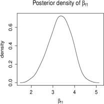
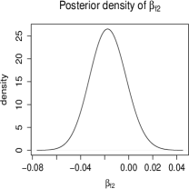
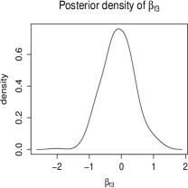
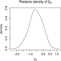
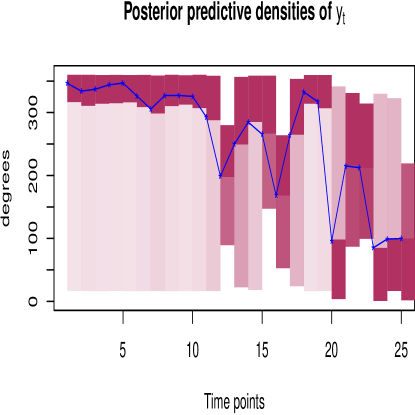
Figures 1 and 2 depict the posterior densities of the four components of $\mbox{\boldmath{$\beta$}}_{f}$ and the first two components of $\mbox{\boldmath{$\beta$}}_{g}$, respectively. The posterior predictive densities of $x_{101}$ and $y_{101}$ are provided in Figure 3. The horizontal bold black lines denote the 95% highest posterior density credible intervals and the vertical lines denote the true values. We observe that the true values of $y_{101}$ and $x_{101}$ fall well within the respective intervals.

It is seen that the densities of most of $x_{t}$, $t=1,\ldots,T,$ have multiple modes. So, a plot of the posterior probability distribution of the latent process for each time point is more appropriate than ordinary credible regions. Such a plot for the latent circular time series $x_{1},\dots,x_{T}$ is displayed in Figure 4. In this plot, regions with progressively higher densities are shown by progressively more intense colors. Encouragingly, most of the true values are seen to lie in the high probability regions.

Figure 1: Posterior densities of the four components of $\mbox{\boldmath{$\beta$}}_{f}$ for simulated data.

Figure 2: Posterior densities of the first and second components of $\mbox{\boldmath{$\beta$}}_{g}$ for simulated data.

Figure 3: From left: The first panel displays the posterior predictive density of $y_{101}$ of simulated data. The second plot represents the posterior predictive density of $x_{101}$ (last latent observation). The thick horizontal line denotes the 95% highest posterior density credible interval and the vertical line denotes the true value for both the figures.

Figure 4: Depiction of the posterior densities of the latent circular process $\left\{x_{t};t=1,\ldots,T\right\}$; higher the intensity of the color, higher is the posterior density. The blue stars denote the true time series.

4.4.1 Cross-validation

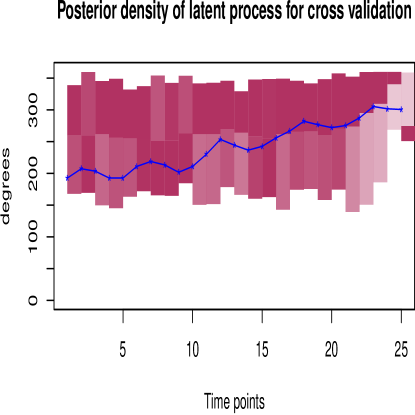
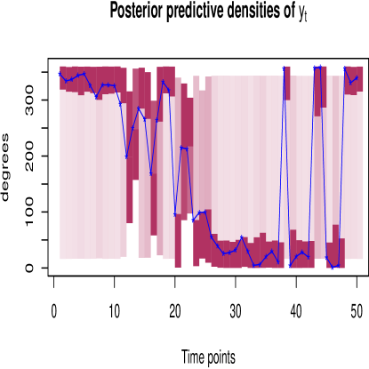
For further validation of our model, we consider detailed leave-one-out cross-validation for three simulated data sets with sample sizes 25, 50 and 100. In each case, at every time point $t$, we set aside $y_{t}$ pretending it to be unobserved and predict the same, for $t=1,\ldots,T$. The colored posterior probability plots for the leave-one-out posterior predictive densities of $\left\{y_{t},~{}t=1,\ldots,T\right\}$, along with the corresponding latent circular process $\left\{x_{t},~{}t=1,\ldots,T\right\}$, are displayed in Figures 5, 6 and 7, respectively, for simulated data with sample sizes 25, 50 and 100. It is very heartening to observe that in almost all the cases, $y_{t}$ and $x_{t}$ fall in high probability regions under the leave-one-out cross-validation scheme. Importantly, one should note that the sample sizes do not have any effect on our proposed methodology.

Thus, in a nutshell, we can claim that our model performs quite optimistically, in spite of the true model being highly non-linear and assumed to be unknown. As a consequence, we expect our model and methods to perform adequately in general situations.

Figure 5: Depiction of the posterior densities of the latent circular process $\left\{x_{t};t=1,\ldots,25\right\}$ and the observed circular process $\left\{y_{t};t=1,\ldots,25\right\}$ under the leave-one-out cross-validation scheme; higher the intensity of the color, higher is the posterior density. The blue stars denote the true time series for $x_{t}$ and $y_{t}$.

Figure 6: Depiction of the posterior densities of the latent circular process $\left\{x_{t};t=1,\ldots,50\right\}$ and the observed circular process $\left\{y_{t};t=1,\ldots,50\right\}$ under the leave-one-out cross-validation scheme; higher the intensity of the color, higher is the posterior density. The blue stars denote the true time series for $x_{t}$ and $y_{t}$.

Figure 7: Depiction of the posterior densities of the latent circular process $\left\{x_{t};t=1,\ldots,100\right\}$ and the observed circular process $\left\{y_{t};t=1,\ldots,100\right\}$ under the leave-one-out cross-validation scheme; higher the intensity of the color, higher is the posterior density. The blue stars denote the true time series for $x_{t}$ and $y_{t}$.

5 Model validation with real data analysis

In this section we validate our methodologies by applying them to two real circular time series data where the time-varying and circular covariates are originally known but we assume to be unknown. In other words, we attempt to predict the circular covariates considering them to be unobserved latent variables.

5.1 Wind pair data

5.1.1 Brief description of the data

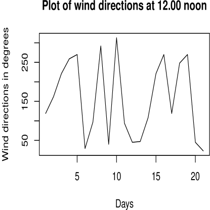
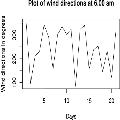
Our first data set consists of a pair of wind directions recorded at $6.00$ am and $12.00$ noon for each of twenty one consecutive days at a weather station in Milwaukee. This data set, which is taken from Fisher (1993) (see page $253$ of Fisher (1993) for more details of the data), is originally recorded in degrees; for our convenience, we converted them to radians ranging from $0$ to $2\pi$. Here we consider the wind directions at $6.00$ am to be the latent circular variables and those at $12.00$ noon, to be the observed variables. Moreover, we use 20 observations for our analysis and set aside the last observation for the purpose of forecasting. In this study we are mainly interested in demonstrating how well our model is able to capture the recorded, real, wind direction data observed at $6.00$ am, considered to be latent relative to our model. Plots of the true wind directions at both the time points for 21 days are provided in Figure 8.

5.1.2 Prior choices and MCMC implementations

We choose the prior means of $\mbox{\boldmath{$\beta$}}_{f}$ and $\mbox{\boldmath{$\beta$}}_{g}$ to be $(0,0,0,0)^{\prime}$ and $(1,1,1,1)^{\prime}$, respectively. As regards the prior covariance matrices of $\mbox{\boldmath{$\beta$}}_{f}$ and $\mbox{\boldmath{$\beta$}}_{g}$, we consider the identity matrix of dimension 4 and a diagonal matrix with diagonal entries $(1,1,0,0)^{\prime}$, respectively. To avoid identifiability issues, we fix the last two components of $\mbox{\boldmath{$\beta$}}_{g}$ at $1$.

The MLEs of $\sigma_{f}$, $\sigma_{\epsilon}$, $\sigma_{g}$ and $\sigma_{\eta}$, which are calculated using simulated annealing and assumed to be known thereafter, turned out to be $2.74891$, $0.30649$, $0.71260$ and $0.36719$, respectively. Using these prior parameters we run $3.5\times 10^{5}$ MCMC iterations and store the last $50,000$ observations for inference, discarding the first $3\times 10^{5}$ as burn in. The time taken by our server machine to implement $3.5\times 10^{5}$ iterations of our MCMC algorithm is 11 hours 47 minutes.

5.1.3 Model fitting results

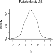
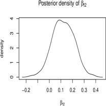
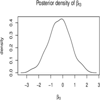
The posterior densities of the four components of the vector $\mbox{\boldmath{$\beta$}}_{f}$ and the two components of $\mbox{\boldmath{$\beta$}}_{g}$ are provided in Figures 9 and 10, respectively, and the posterior predictive densities of $y_{21}$ and $x_{21}$ are displayed in Figure 12. It is observed that the true values of $y_{21}$ and $x_{21}$ fall well within the 95% highest posterior density credible intervals, clearly demonstrating how well our model and the prior distributions of the parameters successfully describe the uncertainty present in the data. The marginal posterior densities of the latent variables are shown in Figure 11, where progressively higher intensities of the color denote regions of progressively higher posterior densities, and the blue stars stand for the true values of the wind directions at time $6.00$ am. It is noted that the true values of the latent variable, namely, the wind directions at time $6.00$ am (in radians), fall mostly in the respective high probability regions. Our Bayesian model and methods are particularly impressive in the sense that the highly nonlinear trend of the latent variable is adequately captured even when the data size is only 20. Since our nonparametric ideas permit the unknown observational and evolutionary function, based on Gaussian processes, to change with time, such encouraging performance is not surprising.

Figure 8: Plot of the wind directions at 12.00 noon and 6.00 am for 21 days.

Figure 9: Posterior densities of the four components of $\mbox{\boldmath{$\beta$}}_{f}$ for the wind pair data.

Figure 10: Posterior densities of the first two components of $\mbox{\boldmath{$\beta$}}_{g}$ for the wind pair data.

Figure 11: Representation of the marginal posterior densities of the latent variables corresponding to wind directions at 6.00 am as a color plot; progressively higher densities are represented by progressively intense colors. The blue stars represent the true wind directions (at 6.00 am) data.

Figure 12: From left: The first panel displays the posterior predictive density of the $21$st observation of wind directions at 12.00 noon for the wind pair data. The second plot represents the posterior predictive density of the 21st observation of wind direction at 6.00 am (latent variable). The thick horizontal line denotes the 95% highest posterior density credible interval and the vertical line denotes the true value (in radian) for both the panels.

5.1.4 Cross-validation results

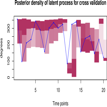
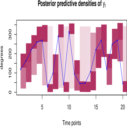
We now present the results of leave-one-out cross-validation for the wind pair data. As in the simulation studies, here we predict wind directions at time $12.00$ pm for 20 days, assuming that the variable is not observed on the $t$-th day, $t=1,\ldots,20$. We also record the posterior distribution of the corresponding latent process, namely, wind directions at time $6.00$ am. The posterior densities are depicted in Figure 13 for both the observed and latent circular processes. As expected, the true values of both the wind directions fall in the high probability regions in almost all the cases.

Figure 13: Depiction of the posterior densities of the latent circular process wind direction at time $6.00$ am for 20 days and the observed circular process wind direction at time $12.00$ pm for 20 days under the leave-one-out cross-validation scheme; higher the intensity of the color, higher is the posterior density. The blue stars denote the true values.

5.2 Spawning time and low tide time data

5.2.1 A brief description of the data set

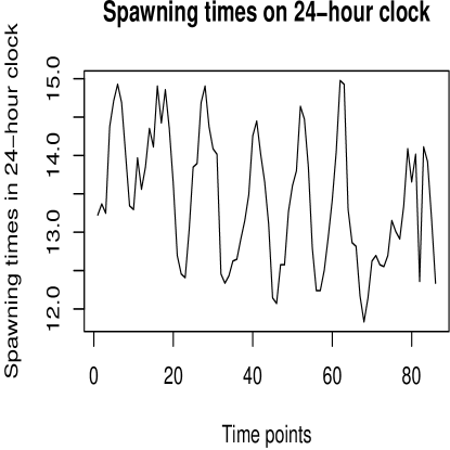
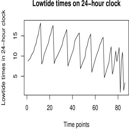
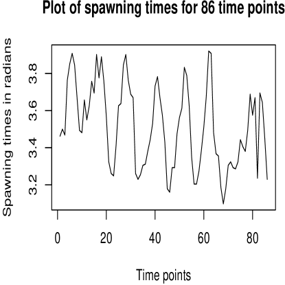
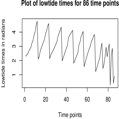
We apply our model and methodology to another real data set for the purpose of validation. Robert R. Warner at the University of California collected data on the spawning times of a particular fish in a marine biology study (see Lund (1999)). It is seen that the spawning time of a fish is influenced by the tidal characteristic of the fish’s local environment. A regression study was done by Lund (1999) considering spawning time as dependent variable and time of low tide as the covariate. There are 86 observations for spawning times and low tide times. The plots of both the variables on the 24-hour clock scale are provided in Figure 14. We wrap the spawning time points and low tide time points on the $(0,2\pi]$ scale (a corresponding plot is given in Figure 15) for our analysis. For our model we assume that the low tide times are latent and spawning times are observed. We use 85 observations for our analysis and set aside the last observation for the prediction purpose. As in Section 5.1 here also our main aim is to show that our methodology is equipped enough to capture the recorded low tide times, considered to be latent with respect to our model.

5.2.2 Prior choices and MCMC implementations for spawning time data

In this example, we choose the prior means of $\mbox{\boldmath{$\beta$}}_{f}$ and $\mbox{\boldmath{$\beta$}}_{g}$ to be $(0,0,0,0)^{\prime}$ and $(0,1.25,1,1)^{\prime}$, and the prior covariance matrices for $\mbox{\boldmath{$\beta$}}_{f}$ and $\mbox{\boldmath{$\beta$}}_{g}$ to be the identity matrix of dimension 4 and a diagonal matrix with diagonal entries $(1,1,0,0)^{\prime}$, respectively, the latter matrix signifying, as usual, our attempt to resolve identifiability problems. The MLEs of $\sigma_{f}$, $\sigma_{\epsilon}$, $\sigma_{g}$ and $\sigma_{\eta}$, obtained by simulated annealing, turned out to be $1.97462$, $0.37569$, $0.67960$ and $0.31686$, respectively. We implemented $2.5\times 10^{5}$ iterations of our MCMC algorithm, storing the last $50,000$ observations for inference. The time taken by our server machine to implement this exercise is 18 hours 54 minutes.

5.3 Results and discussions on the spawning time data

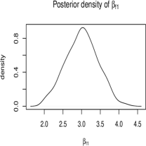
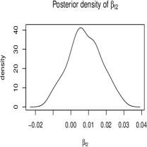
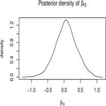
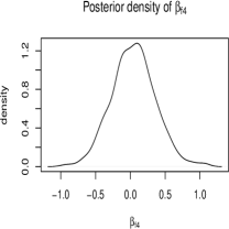
We provide the plots of the posterior densities of the four components of $\mbox{\boldmath{$\beta$}}_{f}$ for the spawning time data in Figure 16 and those of the two components of $\mbox{\boldmath{$\beta$}}_{g}$ are displayed in Figure 17. The posterior densities of the latent variables, that is, low tide times, are depicted in Figure 18. As in the previous experiment, here also it is seen that the posterior densities of the latent variables are highly multimodal. The plots of the posterior densities of the latent process for all the time points are presented in Figure 18, where the observed values of the low tide times are denoted by the blue colored stars. Encouragingly, all the true values, except only the first three points, fall in the high probability density regions. Finally the posterior predictive densities of $x_{86}$ and $y_{86}$, displayed in Figure 19, show that the true values of $x_{86}$ and $y_{86}$ fall well within the 95% highest posterior probability density region. We have conducted the usual tests of MCMC convergence diagnostics, all of which turned out to be satisfactory.

Figure 14: Plots of spawning times of a fish and low tide times on the 24-hour clock.

Figure 15: Plots of spawning times of a fish and low tide times after wrapping on $(0,2\pi]$.

Figure 16: Posterior densities of the four components of $\mbox{\boldmath{$\beta$}}_{f}$ for the spawning time data.

Figure 17: Posterior densities of the first two components of $\mbox{\boldmath{$\beta$}}_{g}$ for the spawning time data.

Figure 18: Representation of the marginal posterior densities of the latent variables corresponding to 85 low tide times as a color plot; progressively higher densities are represented by progressively intense colors. The blue stars represent the true low tide timings (in degrees).

Figure 19: The left panel displays the posterior predictive density of the $86$-th observation for the spawning time. The right panel depicts the posterior predictive density of the $86$-th observation for low tide time. For both the plots, the thick horizontal line denotes the 95% highest posterior density credible interval and the vertical line denotes the true value (in radian).

5.3.1 Results of cross-validation

As earlier cases of simulation and wind pair data, here we predict the spawning times for 85 observations, setting aside the $t$-th spawning time, $t=1,\ldots,85$, as unobserved; we also record, as before, the posteriors of the $t$-th low tide time, the corresponding latent variable. The relevant cross-validation posterior densities along with the true time series, are displayed in Figure 20. Once again, the results have been highly encouraging.

Figure 20: Depiction of the posterior densities of the latent circular process, low tide times for 85 observations, and that of the observed circular process, spawning time for 85 observations, under the leave-one-out cross-validation scheme; higher the intensity of the color, higher is the posterior density. The blue stars denote the true values.

6 Application to whale positional data

6.1 A brief description of the data set

An interesting data set on whale movement directions is available at http://nbviewer.jupyter.org/github/robertodealmeida/notebooks/blob/master/earth_day_data_challenge/Analyzing%20whale%20tracks.ipynb , on which we apply our model and methodologies to predict the directions of the ocean current.

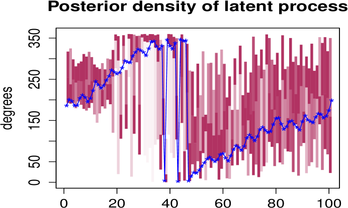
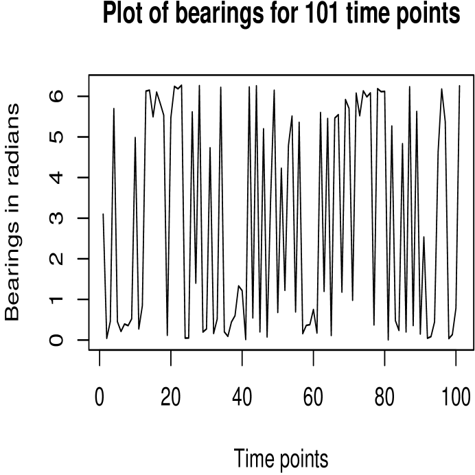
Specifically, in this website 242 positions of a whale has been recorded in terms of latitudes and longitudes. The whale began its migration on 24th December of 2003 at the position 20.465 S, 40.04 W, and ended on 28th February of 2004 at 54.67 S, 26.261 W. This was an experimental project by Roberto De Almeida, who was interested whether whales could benefit from the ocean currents while migrating. For our purpose, first we processed the raw data by calculating the angles between these latitudes and longitudes, known as bearing, using the formula given in http://www.movable-type.co.uk/scripts/latlong.html. Finally, we obtained 241 circular univariate angular observations in radians. To reduce computational complexity here we have considered only the first 100 observations for our analysis setting aside the 101-th observation for the purpose of prediction. A plot of the first 101 bearings is shown in Figure 21. It is expected that the positions of the whale depends upon the directions of the ocean current, but the latter are not recorded. Hence, we anticipate that our general, nonparametric model and its corresponding methods will provide useful predictions of the direction of the ocean current, even though only the whale positions are observed.

6.2 Prior choices and MCMC implementation

The means of the prior distributions of $\mbox{\boldmath{$\beta$}}_{f}$ and $\mbox{\boldmath{$\beta$}}_{g}$ are set as $(5,5,5,5)^{\prime}$ and $(0,2,1,1)^{\prime}$, respectively, and their covariance matrices are as before considered to be the $4\times 4$ identity matrix and the diagonal matrix with the diagonal entries $(1,1,0,0)^{\prime}$. We made these choices to ensure adequate mixing of our MCMC chain. The MLEs of $\sigma_{f}$, $\sigma_{\epsilon}$, $\sigma_{g}$ and $\sigma_{\eta}$ are found to be $1.15391$, $0.24421$, $0.19264$ and $0.26019$, respectively, using simulated annealing.

With these choices of prior parameters we implemented $2.5\times 10^{5}$ iterations of our MCMC algorithm, storing the last 50,000 observations for inference. The entire exercise took 25 hours 31 minutes in our server computer. The usual tests for convergence of MCMC indicated adequate mixing properties.

6.3 Results of the whale positional data

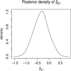
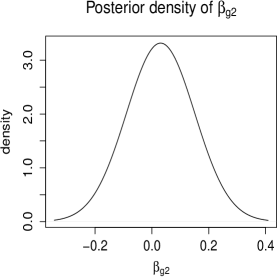
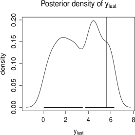
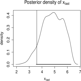
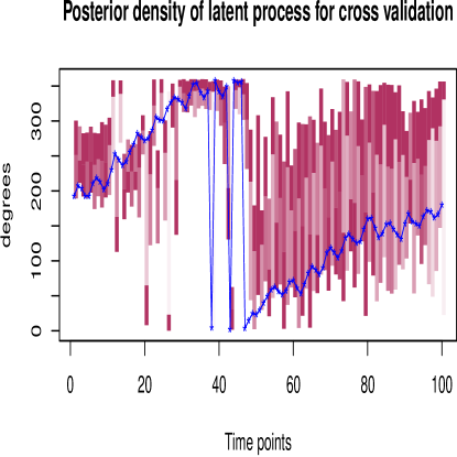
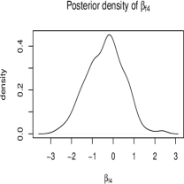
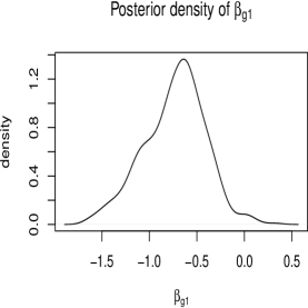
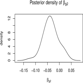
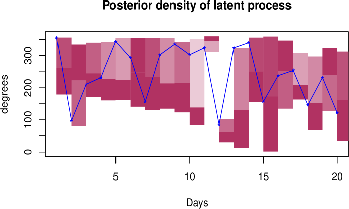
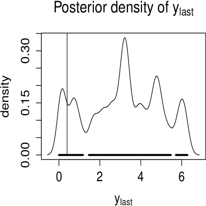
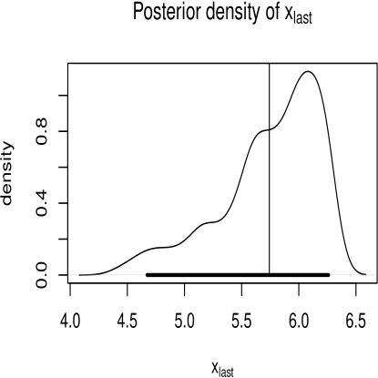
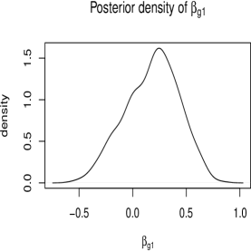
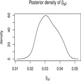
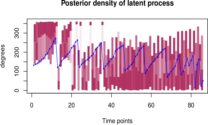
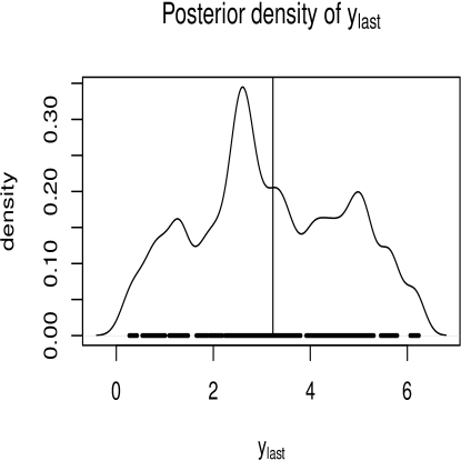
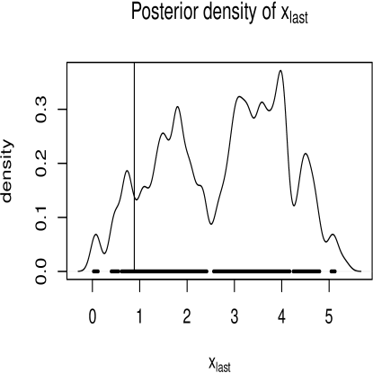
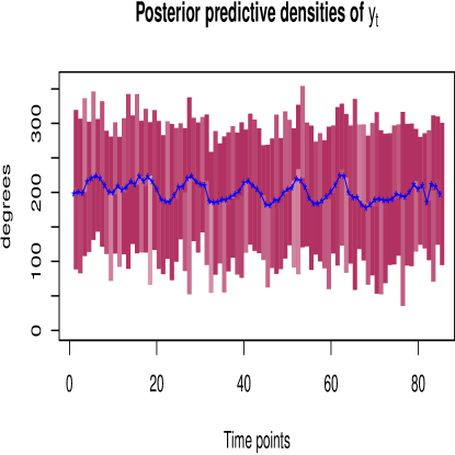
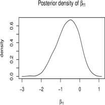
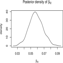
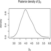
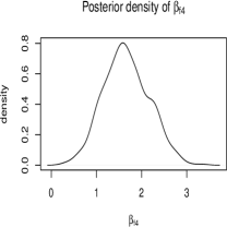
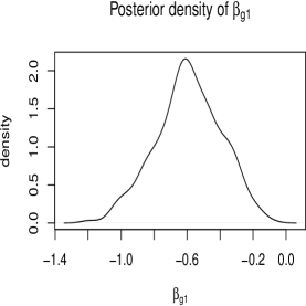
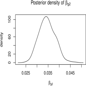
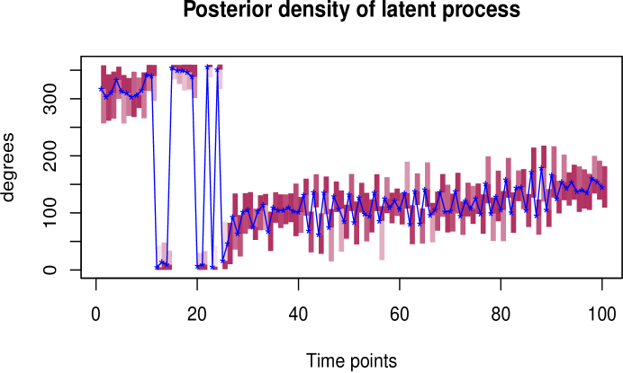
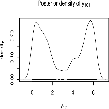
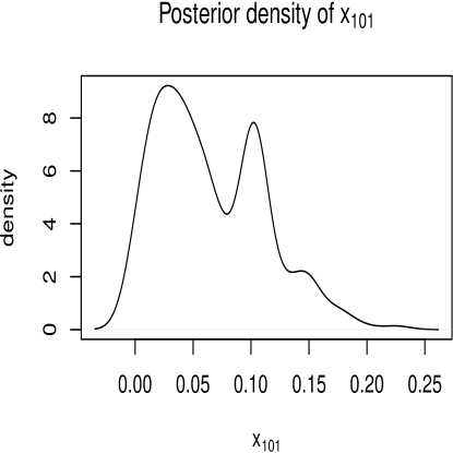
We provide the plots of posterior densities of four components of $\mbox{\boldmath{$\beta$}}_{f}$ and two components of $\mbox{\boldmath{$\beta$}}_{g}$ in Figures 22 and 23, respectively. Figure 24 shows the marginal posterior distributions associated with the latent circular process depicted by progressively intense colors. In Figure 24, the blue stars indicate the posterior medians of the latent process. Finally, the posterior predictive densities corresponding to $y_{101}$ and $x_{101}$ are shown in Figure 25. The thin vertical line in the left panel denotes the true value of the $101$-th observation of the bearing value and the thick, broken line on the horizontal axis represents the 95% highest density region of the posterior predictive density of $y_{101}$. As in our previous experiments, here also the true value falls well within the 95% highest posterior density credible interval. Thus, overall, the performance of our model and methods seems to be quite satisfactory.

Figure 21: Plots of the bearings for 101 time points of the whale positions.

Figure 22: Posterior densities of the four components of $\mbox{\boldmath{$\beta$}}_{f}$ for the whale positional data.

Figure 23: Posterior densities of the first two components of $\mbox{\boldmath{$\beta$}}_{g}$ for the whale positional data.

Figure 24: Depiction of the marginal posterior distributions of the latent variables using progressively intense colors for progressively higher densities. The blue stars represent the posterior medians of the latent process.

Figure 25: The left panel shows the posterior predictive density of the $101$-th observation of bearing of the whale positional data. The thick horizontal line denotes the 95% highest posterior density credible interval and the vertical line denotes the true value. The right panel displays the posterior predictive density of the 101-th observation of the direction of ocean current.

6.4 Cross-validation results

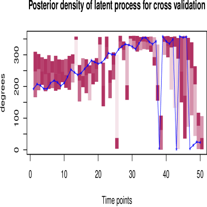
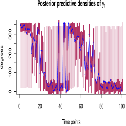
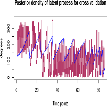
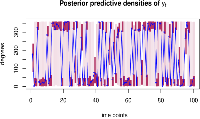
In the leave-one-out cross-validation exercise for the whale positional data, we provide the results only for the observed data, since, unlike the previous experiments, the true values associated with the latent process are unknown. The posterior densities of the 100 bearings are displayed in Figure 26, and as expected, the results have been highly encouraging.

Figure 26: Depiction of the posterior densities of the observed circular process, bearings of whale positions for 100 time points, under the leave-one-out cross-validation scheme; higher the intensity of the color, higher is the posterior density. The blue stars denote the true values.

7 Discussion and conclusion

In nature there exist plentiful examples of circular time series where the underlying influential circular variable remains unrecorded. Some such examples, apart from the whale movement directions considered in this paper, are directions of flights of birds and missiles, where the underlying wind directions, although affects the flight directions, generally remains unrecorded. Modeling such circular time series using traditional parametric and nonparametric methods existing in the literature (for example, methods proposed in Breckling (1989), Fisher and Lee (1994), Holzmann et al. (2006), Hughes (2007), Di Marzio et al. (2012)) will be far less effective compared to state space approaches that treat the underlying unrecorded process as a latent circular process. In this regard, we have introduced and developed a novel Bayesian nonparametric state space model for circular time series where the latent states also constitute a circular process.

Moreover, since it is clearly non-trivial to model general circular time series accounting for adequate non-Markov angular dependence structure, our endeavor seems to facilitate significant advance in this respect. Indeed, the observed time series in our state space model has a complex and realistic dependence structure, facilitated by the circular latent state process along with the structures induced by the wrapped Gaussian process, even though conditionally on the latent states and the observational function we assume the circular observations to be independent and further assume a Markovian structure of the latent states conditional on the look-up table. These structures within our state space model facilitates an effective MCMC procedure, while ensuring highly realistic dependence structure. Such realistically complex dependence structures are absent in the traditional parametric and nonparametric circular time series models existing in the literature.

Other than our current work, the only research on state space models that considers circular latent states is that of Mazumder and Bhattacharya (2016a); however, they assume that the observed time series is associated with a linear process, unlike our observed circular time series. The observed circular process, as we argued, gave rise to significantly more complexities and difficult technical challenges in our case, compared to that of Mazumder and Bhattacharya (2016a). However, the complexities of our Bayesian model and methods notwithstanding, we have amply demonstrated with simulation studies as well as with three real data sets, the effectiveness of our proposed procedures.

Ideally, it seems that comparison of our proposed model and methods with the existing works is desirable, but for circular times series such comparison does not seem to be possible. We explain this as follows. Most linear time series admit state-space representation, where both the observational and evolutionary equations are defined on the real line. However, it is unclear if the existing circular time series admit state-space representation. Even if some of them do, it is unlikely that the corresponding latent states will be circular. This is because for circular latent states, it is unlikely that marginalization over the circular latent states is analytically possible to arrive at the known forms of the existing circular time series. The difficulty of marginalization stems from the need to integrate complex expressions over the bounded domain $(0,2\pi]$. We are not aware of any existing circular time series that admits a state space representation with circular latent states. Since the main assumption of our model is that there is an underlying circular latent structure, it seems that comparison of the existing methods with our method is not possible.

Note that there perhaps exists a much larger class of circular time series in nature which depend upon unrecorded linear processes, necessitating the development of Bayesian nonparametric state space models with observed circular process and latent linear process. But such development is a much simpler exercise given our current work and the developments provided in Ghosh et al. (2014). As more interesting alternatives, we shall focus on developing Bayesian nonparametric state space models and methods when the observed times series and the latent states are multivariate, with several linear and several circular components.

Supplementary Material

S-1 Full conditional distributions of $\mbox{\boldmath{$\beta$}}_{f}$

$$[\mbox{\boldmath{$\beta$}}_{f}|\ldots] \propto[\mbox{\boldmath{$\beta$}}_{f}][\mbox{\boldmath{$f$}}^{*}|x_{1},\ldots,x_{T+1},\mbox{\boldmath{$\beta$}}_{f},\sigma_{f}]$$

$$\propto\exp\left\{-\frac{1}{2}(\mbox{\boldmath{$\beta$}}_{f}-\mbox{\boldmath{$\beta$}}_{f,0})^{\prime}\Sigma^{-1}_{\mbox{\boldmath{$\beta$}}_{f,0}}(\mbox{\boldmath{$\beta$}}_{f}-\mbox{\boldmath{$\beta$}}_{f,0})-\frac{1}{2}(\mbox{\boldmath{$f$}}^{*}-\mbox{\boldmath{$H$}}\mbox{\boldmath{$\beta$}}_{f})^{\prime}\sigma^{-2}_{f}\mbox{\boldmath{$A$}}_{f}^{-1}(\mbox{\boldmath{$f$}}^{*}-\mbox{\boldmath{$H$}}\mbox{\boldmath{$\beta$}}_{f})\right\}$$

$$\propto\exp\left\{-\frac{1}{2}\left[\mbox{\boldmath{$\beta$}}_{f}^{\prime}\left(\Sigma^{-1}_{\mbox{\boldmath{$\beta$}}_{f,0}}+\mbox{\boldmath{$H$}}^{\prime}\sigma^{-2}_{f}A^{-1}_{f}\mbox{\boldmath{$H$}}\right)\mbox{\boldmath{$\beta$}}_{f}-2\mbox{\boldmath{$\beta$}}_{f}^{\prime}\left(\Sigma^{-1}_{\mbox{\boldmath{$\beta$}}_{f,0}}\mbox{\boldmath{$\beta$}}_{f,0}+\mbox{\boldmath{$H$}}^{\prime}\sigma^{-2}_{f}\mbox{\boldmath{$A$}}_{f}^{-1}\mbox{\boldmath{$f$}}^{*}\right)\right]\right\},$$ (20)

where $\mbox{\boldmath{$H$}}=\left[\mbox{\boldmath{$h$}}(1,x_{1})^{\prime},\ldots,\mbox{\boldmath{$h$}}(T+1,x_{T+1})^{\prime}\right]^{\prime}$. Therefore, the full conditional distribution of $\mbox{\boldmath{$\beta$}}_{f}$ is a four-variate normal distribution with mean

$$E[\mbox{\boldmath{$\beta$}}_{f}|\ldots]=\left(\Sigma^{-1}_{\mbox{\boldmath{$\beta$}}_{f,0}}+\mbox{\boldmath{$H$}}^{\prime}\sigma^{-2}_{f}A^{-1}_{f}\mbox{\boldmath{$H$}}\right)^{-1}\left(\Sigma^{-1}_{\mbox{\boldmath{$\beta$}}_{f,0}}\mbox{\boldmath{$\beta$}}_{f,0}+\mbox{\boldmath{$H$}}^{\prime}\sigma^{-2}_{f}\mbox{\boldmath{$A$}}_{f}^{-1}\mbox{\boldmath{$f$}}^{*}\right)$$ (21)

and variance covariance matrix

$$V[\mbox{\boldmath{$\beta$}}_{f}|\ldots]=\left(\Sigma^{-1}_{\mbox{\boldmath{$\beta$}}_{f,0}}+\mbox{\boldmath{$H$}}^{\prime}\sigma^{-2}_{f}A^{-1}_{f}\mbox{\boldmath{$H$}}\right)^{-1}.$$ (22)

To update $\mbox{\boldmath{$\beta$}}_{f}$ we use Gibbs sampling.

S-2 Full conditional distribution of $\sigma_{f}$

$$[\sigma_{f}^{2}|\ldots] \propto[\sigma_{f}^{2}][\mbox{\boldmath{$f$}}^{*}|x_{1},\ldots,x_{T+1},\mbox{\boldmath{$\beta$}}_{f},\sigma_{f}]$$

$$=(\sigma^{2}_{f})^{-\frac{\alpha_{f}+2+(T+1)}{2}}\exp\left\{-\frac{1}{2\sigma^{2}_{f}}\left[\gamma_{f}+(\mbox{\boldmath{$f$}}^{*}-\mbox{\boldmath{$H$}}\mbox{\boldmath{$\beta$}}_{f})^{\prime}\mbox{\boldmath{$A$}}_{f}^{-1}(\mbox{\boldmath{$f$}}^{*}-\mbox{\boldmath{$H$}}\mbox{\boldmath{$\beta$}}_{f})\right]\right\}.$$ (23)

Since $\mbox{\boldmath{$A$}}_{f}$ involves $\sigma_{f}^{2}$ (recall that $\mbox{\boldmath{$A$}}_{f}$ = ($\exp\left(-\sigma_{f}^{4}(i-j)^{2}\right)\cos(|x_{i}-x_{j}|)$)) so, the closed form of the above posterior density is not tractable. Therefore, we use a random walk Metropolis-Hastings step to update $\sigma^{2}_{f}$.

S-3 Full conditional density of $\sigma_{\epsilon}$

$$[\sigma_{\epsilon}^{2}] \propto[\sigma_{\epsilon}^{2}]\prod_{t=1}^{T}[N_{t}|f^{*}(t,x_{t}),\sigma_{\epsilon},x_{t}]\prod_{t=1}^{T}[y_{t}|N_{t},f^{*}(t,x_{t}),\sigma_{\epsilon},x_{t}]$$

$$\propto(\sigma^{2}_{\epsilon})^{-\frac{\alpha_{\epsilon}+2+T}{2}}\exp\left\{-\frac{1}{2\sigma^{2}_{\epsilon}}\sum_{t=1}^{T}(y_{t}+2\pi N_{t}-f^{*}(t,x_{t}))^{2}\right\}.$$ (24)

Therefore, the full conditional distribution of $\sigma_{\epsilon}^{2}$ is inverse gamma with the parameters $\frac{\alpha_{\epsilon}+T}{2}$ and
$\frac{\sum_{t=1}^{T}(y_{t}+2\pi N_{t}-f^{*}(t,x_{t}))^{2}}{2}$. Thus, we use the Gibbs sampling technique to update $\sigma^{2}_{\epsilon}$.

S-4 Full conditional density of $\mbox{\boldmath{$f$}}_{\mbox{\scriptsize$D_{T}$}}^{*}$

$$[\mbox{\boldmath{$f$}}_{\mbox{\scriptsize$D_{T}$}}^{*}|\ldots] \propto[\mbox{\boldmath{$f$}}_{\mbox{\scriptsize$D_{T}$}}^{*}|x_{1},\ldots,x_{T+1},\mbox{\boldmath{$\beta$}}_{f},\sigma_{f}]\prod_{t=1}^{T}[N_{t}|f^{*}(t,x_{t}),\sigma_{\epsilon},x_{t}]\prod_{t=1}^{T}[y_{t}|N_{t},f^{*}(t,x_{t}),\sigma_{\epsilon},x_{t}]$$

$$\propto\exp\left\{-\frac{1}{2}(\mbox{\boldmath{$f$}}_{\mbox{\scriptsize$D_{T}$}}^{*}-\mbox{\boldmath{$H$}}_{\mbox{\scriptsize$D_{T}$}}\mbox{\boldmath{$\beta$}}_{f})^{\prime}\sigma^{-2}_{f}\mbox{\boldmath{$A$}}_{f,D_{T}}^{-1}(\mbox{\boldmath{$f$}}_{\mbox{\scriptsize$D_{T}$}}^{*}-\mbox{\boldmath{$H$}}_{\mbox{\scriptsize$D_{T}$}}\mbox{\boldmath{$\beta$}}_{f})-\frac{1}{2\sigma^{2}_{\epsilon}}\sum_{t=1}^{T}(y_{t}+2\pi N_{t}-f^{*}(t,x_{t}))^{2}\right\}$$

$$\propto\exp\left\{-\frac{1}{2}\left[\mbox{\boldmath{$f$}}_{\mbox{\scriptsize$D_{T}$}}^{*}\left(\sigma^{-2}_{f}\mbox{\boldmath{$A$}}_{f,D_{T}}^{-1}+\sigma^{-2}_{\mbox{\scriptsize$\epsilon$}}I_{T}\right)\mbox{\boldmath{$f$}}_{\mbox{\scriptsize$D_{T}$}}^{*}-2\mbox{\boldmath{$f$}}_{\mbox{\scriptsize$D_{T}$}}^{*}\left(\sigma^{-2}_{f}\mbox{\boldmath{$A$}}_{f,D_{T}}^{-1}\mbox{\boldmath{$H$}}_{\mbox{\scriptsize$D_{T}$}}\mbox{\boldmath{$\beta$}}_{f}+\sigma^{-2}_{\mbox{\scriptsize$\epsilon$}}[\mbox{\boldmath{$D$}}_{T}+2\pi\mbox{\boldmath{$N$}}]\right)\right]\right\},$$ (25)

where $\mbox{\boldmath{$D$}}_{T}+2\pi\mbox{\boldmath{$N$}}$ = $(y_{1}+N_{1},\ldots,y_{T}+N_{T})^{\prime}$. Hence, $[\mbox{\boldmath{$f$}}_{\mbox{\scriptsize$D_{T}$}}^{*}|\ldots]$ is a $T$-variate normal distribution with the parameters

$$E[\mbox{\boldmath{$f$}}_{\mbox{\scriptsize$D_{T}$}}^{*}|\ldots]=\left(\sigma^{-2}_{f}\mbox{\boldmath{$A$}}_{f}^{-1}+\sigma^{-2}_{\mbox{\scriptsize$\epsilon$}}I_{T}\right)^{-1}\left(\sigma^{-2}_{f}\mbox{\boldmath{$A$}}_{f,D_{T}}^{-1}\mbox{\boldmath{$H$}}_{\mbox{\scriptsize$D_{T}$}}\mbox{\boldmath{$\beta$}}_{f}+\sigma^{-2}_{\mbox{\scriptsize$\epsilon$}}[\mbox{\boldmath{$D$}}_{T}+2\pi\mbox{\boldmath{$N$}}]\right)$$ (26)

and

$$\mbox{cov}[\mbox{\boldmath{$f$}}_{\mbox{\scriptsize$D_{T}$}}^{*}|\ldots]=\left(\sigma^{-2}_{f}\mbox{\boldmath{$A$}}_{f,D_{T}}^{-1}+\sigma^{-2}_{\mbox{\scriptsize$\epsilon$}}I_{T}\right)^{-1}.$$ (27)

Hence, we use the Gibbs sampling technique to update $\mbox{\boldmath{$f$}}_{\mbox{\scriptsize$D_{T}$}}^{*}$.

S-5 Full conditional distribution of $f^{*}(T+1,x_{T+1})$

$$[f^{*}(T+1,x_{T+1})|\ldots]\propto[f^{*}(T+1,x_{T+1})|\mbox{\boldmath{$f$}}_{\mbox{\scriptsize$D_{T}$}}^{*},x_{T+1},\mbox{\boldmath{$\beta$}}_{f},\sigma_{f}].$$ (28)

Hence, $[f^{*}(T+1,x_{T+1})|\ldots]$ follows the univariate normal distribution with parameters $\mu_{\mbox{\scriptsize$f^{*}(T+1,x_{T+1})$}}$ and variance $\sigma_{\mbox{\scriptsize$f^{*}(T+1,x_{T+1})$}}^{2}$, and so, we update $f^{*}(T+1,x_{T+1})$ by Gibbs sampling.

S-6 Full conditional density of $N_{t}$, $t=1,\ldots,T$

$$[N_{t}|\ldots] \propto[N_{t}|f^{*}(t,x_{t}),\sigma_{\mbox{\scriptsize$\epsilon$}},x_{t}][y_{t}|N_{t},f^{*}(t,x_{t}),\sigma_{\mbox{\scriptsize$\epsilon$}},x_{t}]$$

$$\propto\exp{\left(-\frac{1}{2\sigma^{2}_{\mbox{\scriptsize$\epsilon$}}}(y_{t}+2\pi N_{t}-f^{*}(t,x_{t}))^{2}\right)}I_{\{\ldots,-1,0,1,\ldots\}}(N_{t}),~{}t=1,\ldots,T.$$ (29)

The full conditional distribution of $N_{t}$, $t=1,\ldots,T$, are not tractable, and so we update them by random walk Metropolis-Hastings steps.

S-7 Full conditional density of $\mbox{\boldmath{$\beta$}}_{g}$

$$[\mbox{\boldmath{$\beta$}}_{g}|\cdots] \propto[\mbox{\boldmath{$\beta$}}_{g}][\mbox{\boldmath{$D$}}_{z},g^{*}(1,x_{0})|x_{0},\mbox{\boldmath{$\beta$}}_{g},\sigma^{2}_{g}]\prod_{t=2}^{T+1}[x_{t}|\mbox{\boldmath{$\beta$}}_{g},\sigma^{2}_{\mbox{\scriptsize$\eta$}},\sigma^{2}_{g},\mbox{\boldmath{$D$}}_{z},x_{t-1},K_{t}]\prod_{t=2}^{T+1}\left[K_{t}|\mbox{\boldmath{$\beta$}}_{g},\sigma^{2}_{\mbox{\scriptsize$\eta$}}\right.$$

$$\quad\left.\sigma^{2}_{g},\mbox{\boldmath{$D$}}_{z},x_{t-1}\right]$$ (30)

We write down the right hand side of (S-7) as follows:

$$[\mbox{\boldmath{$\beta$}}_{g}][\mbox{\boldmath{$D$}}_{z},g^{*}(1,x_{0})|x_{0},\mbox{\boldmath{$\beta$}}_{g}]\prod_{t=2}^{T+1}[x_{t}|\mbox{\boldmath{$\beta$}}_{g},\sigma^{2}_{\mbox{\scriptsize$\eta$}},\mbox{\boldmath{$D$}}_{z},x_{t-1},K_{t}]\prod_{t=2}^{T+1}[K_{t}|\mbox{\boldmath{$\beta$}}_{g},\sigma^{2}_{\mbox{\scriptsize$\eta$}},\mbox{\boldmath{$D$}}_{z},x_{t-1}]$$

$$\propto\exp{\left(-\frac{1}{2}(\mbox{\boldmath{$\beta$}}_{g}-\mbox{\boldmath{$\beta$}}_{g,0})^{\prime}\mbox{\boldmath{$\Sigma$}}_{\beta_{g},0}^{-1}(\mbox{\boldmath{$\beta$}}_{g}-\mbox{\boldmath{$\beta$}}_{g,0})\right)}$$

$$\times\exp{\left(-\frac{1}{2}[(\mbox{\boldmath{$D$}}_{z},g^{*})^{\prime}-(\mbox{\boldmath{$H$}}_{D_{z}}\mbox{\boldmath{$\beta$}}_{g},\mbox{\boldmath{$h$}}^{\prime}(1,x_{0}))^{\prime}]^{\prime}\mbox{\boldmath{$A$}}^{-1}_{D_{z},g^{*}(1,x_{0})}[(\mbox{\boldmath{$D$}}_{z},g^{*})^{\prime}-(\mbox{\boldmath{$H$}}_{D_{z}}\mbox{\boldmath{$\beta$}}_{g},\mbox{\boldmath{$h$}}^{\prime}(1,x_{0}))^{\prime}]\right)}$$

$$\quad\times\exp{\left\{-\sum_{i=2}^{T+1}\frac{1}{2\sigma^{2}_{x_{t}}}(x_{t}+2\pi K_{t}-\mu_{x_{t}})^{2}\right\}}\prod_{t=2}^{T+1}I_{[0,2\pi]}(x_{t}),$$ (31)

where $\mbox{\boldmath{$H$}}_{D_{z}}=\left(\mbox{\boldmath{$h$}}(t_{1},z_{1}),\ldots,\mbox{\boldmath{$h$}}(t_{n},z_{n})\right)^{\prime}$, $\mbox{\boldmath{$A$}}_{D_{z},g^{*}(1,x_{0})}$ is $(n+1)\times(n+1)$ matrix defined as

$$\mbox{\boldmath{$A$}}_{D_{z},g^{*}(1,x_{0})}=\left[\begin{array}[]{c c}\mbox{\boldmath{$A$}}_{g,D_{z}}&\mbox{\boldmath{$s$}}_{g,D_{z}}(1,x_{0})\\ \mbox{\boldmath{$s$}}_{g,D_{z}}(1,x_{0})^{\prime}&\sigma^{2}_{g}\end{array}\right],$$

$\mu_{x_{t}}=\mbox{\boldmath{$h$}}(t,x_{t-1})^{\prime}\mbox{\boldmath{$\beta$}}_{g}+\mbox{\boldmath{$s$}}_{g,D_{z}}(t,x_{t-1})^{\prime}\mbox{\boldmath{$A$}}_{g,D_{z}}^{-1}(\mbox{\boldmath{$D$}}_{z}-\mbox{\boldmath{$H$}}_{D_{z}}\mbox{\boldmath{$\beta$}}_{g})$ and $\sigma^{2}_{x_{t}}=\sigma^{2}_{\mbox{\scriptsize{$\eta$}}}+{\sigma_{g}^{2}}(1-(\mbox{\boldmath{$s$}}_{g,D_{z}}(t,x_{t-1}))^{\prime}\mbox{\boldmath{$A$}}_{g,D_{z}}^{-1}\mbox{\boldmath{$s$}}_{g,D_{z}}(t,\\ x_{t-1}))$, with $\mbox{\boldmath{$A$}}_{g,D_{z}}$ being a $n\times n$ matrix having $(i,j)$th element as $c_{g}((t_{i},z_{i}),(t_{j},z_{j}))$ and with $\mbox{\boldmath{$s$}}_{g,D_{z}}(\cdot,\cdot)=(c_{g}((\cdot,\cdot),(t_{1},z_{1})),\ldots,c_{g}((\cdot,\cdot),(t_{n},z_{n})))^{\prime}$. Observe that the denominator of $[x_{t}|\mbox{\boldmath{$\beta$}}_{g},\sigma^{2}_{\mbox{\scriptsize$\eta$}},\mbox{\boldmath{$D$}}_{z},x_{t-1},K_{t}]$ cancels with the density of $[K_{t}|\mbox{\boldmath{$\beta$}}_{g},\sigma^{2}_{\mbox{\scriptsize$\eta$}},\mbox{\boldmath{$D$}}_{z},x_{t-1}]$, for each $t=2,\ldots,T+1$. Also, we note that the indicator function does not involve $\mbox{\boldmath{$\beta$}}_{g}$ for any $t=2,\ldots,T+1$. Therefore, after simplifying the exponent terms and ignoring the indicator function we can write

$$[\mbox{\boldmath{$\beta$}}_{g}|\cdots]\propto\exp{\left\{-\frac{1}{2}(\mbox{\boldmath{$\beta$}}_{g}-\mu_{\beta_{g}})^{\prime}\mbox{\boldmath{$\Sigma$}}_{\beta_{g}}^{-1}(\mbox{\boldmath{$\beta$}}_{g}-\mu_{\beta_{g}})\right\}},$$ (32)

where

$$\mu_{\beta_{g}}=E[\mbox{\boldmath{$\beta$}}_{g}|\cdots]=\left\{\mbox{\boldmath{$\Sigma$}}_{\beta_{g},0}^{-1}+\frac{1}{\sigma^{2}_{g}}[\mbox{\boldmath{$H$}}_{D_{z}}^{\prime},\mbox{\boldmath{$h$}}(1,x_{0})]\mbox{\boldmath{$A$}}^{-1}_{D_{z},g^{*}(1,x_{0})}[\mbox{\boldmath{$H$}}_{D_{z}}^{\prime},\mbox{\boldmath{$h$}}(1,x_{0})]^{\prime}\right.$$

$$\left.+\sum_{t=1}^{T}\frac{\left(\mbox{\boldmath{$H$}}_{D_{z}}^{\prime}\mbox{\boldmath{$A$}}^{-1}_{g,D_{z}}\mbox{\boldmath{$s$}}_{g,D_{z}}(t+1,x_{t})-\mbox{\boldmath{$h$}}(t+1,x_{t})\right)\left(\mbox{\boldmath{$H$}}_{D_{z}}^{\prime}\mbox{\boldmath{$A$}}^{-1}_{g,D_{z}}\mbox{\boldmath{$s$}}_{g,D_{z}}(t+1,x_{t})-\mbox{\boldmath{$h$}}(t+1,x_{t})\right)^{\prime}}{\sigma^{2}_{x_{t}}}\right\}^{-1}$$

$$\left\{\mbox{\boldmath{$\Sigma$}}_{\beta_{g},0}^{-1}\mbox{\boldmath{$\beta$}}_{g,0}+\frac{1}{\sigma^{2}_{g}}[\mbox{\boldmath{$H$}}_{D_{z}}^{\prime},\mbox{\boldmath{$h$}}(1,x_{0})]\mbox{\boldmath{$A$}}^{-1}_{D_{z},g^{*}(1,x_{0})}[\mbox{\boldmath{$D$}}_{z},g^{*}(1,x_{0})]\right.$$

$$\left.+\sum_{t=1}^{T}\frac{\left(x_{t+1}+2\pi K_{t+1}-\mbox{\boldmath{$s$}}_{g,D_{z}}(t+1,x_{t})^{\prime}\mbox{\boldmath{$A$}}^{-1}_{g,D_{z}}\mbox{\boldmath{$D$}}_{z}\right)\left(\mbox{\boldmath{$h$}}(t+1,x_{t})-\mbox{\boldmath{$H$}}_{D_{z}}^{\prime}\mbox{\boldmath{$A$}}^{-1}_{g,D_{z}}\mbox{\boldmath{$s$}}_{g,D_{z}}(t+1,x_{t})\right)}{\sigma^{2}_{x_{t}}}\right\}$$ (33)

and

$$\mbox{\boldmath{$\Sigma$}}_{\beta_{g}}=V[\mbox{\boldmath{$\beta$}}_{g}|\cdots]=\left\{\mbox{\boldmath{$\Sigma$}}_{\beta_{g},0}^{-1}+\frac{1}{\sigma^{2}_{g}}[\mbox{\boldmath{$H$}}_{D_{z}}^{\prime},\mbox{\boldmath{$h$}}(1,x_{0})]\mbox{\boldmath{$A$}}^{-1}_{D_{z},g^{*}(1,x_{0})}[\mbox{\boldmath{$H$}}_{D_{z}}^{\prime},\mbox{\boldmath{$h$}}(1,x_{0})]^{\prime}\right.$$

$$\left.+\sum_{t=1}^{T}\frac{\left(\mbox{\boldmath{$H$}}_{D_{z}}^{\prime}\mbox{\boldmath{$A$}}^{-1}_{g,D_{z}}\mbox{\boldmath{$s$}}_{g,D_{z}}(t+1,x_{t})-\mbox{\boldmath{$h$}}(t+1,x_{t})\right)\left(\mbox{\boldmath{$H$}}_{D_{z}}^{\prime}\mbox{\boldmath{$A$}}^{-1}_{g,D_{z}}\mbox{\boldmath{$s$}}_{g,D_{z}}(t+1,x_{t})-\mbox{\boldmath{$h$}}(t+1,x_{t})\right)^{\prime}}{\sigma^{2}_{x_{t}}}\right\}^{-1}.$$ (34)

Hence $[\mbox{\boldmath{$\beta$}}_{g}|\cdots]$ follows a four-variate normal distribution with mean and variance $\mu_{\beta_{g}}$ and $\mbox{\boldmath{$\Sigma$}}_{\beta_{g}}$, respectively. Therefore, we update $\mbox{\boldmath{$\beta$}}_{g}$ by Gibbs sampling.

S-8 Full conditional density of $\sigma^{2}_{\mbox{\scriptsize$\eta$}}$

$$[\sigma^{2}_{\mbox{\scriptsize$\eta$}}|\cdots] \propto[\sigma^{2}_{\mbox{\scriptsize$\eta$}}][x_{1}|g^{*}(1,x_{0}),\sigma^{2}_{\mbox{\scriptsize$\eta$}},K_{1}][K_{1}|g^{*}(1,x_{0}),\sigma^{2}_{\mbox{\scriptsize$\eta$}}]\prod_{t=2}^{T+1}[x_{t}|\mbox{\boldmath{$\beta$}}_{g},\sigma^{2}_{\mbox{\scriptsize$\eta$}},\sigma^{2}_{g},\mbox{\boldmath{$D$}}_{z},x_{t-1},K_{t}]$$

$$\quad~{}\times\prod_{t=2}^{T+1}[K_{t}|\mbox{\boldmath{$\beta$}}_{g},\sigma^{2}_{g},\sigma^{2}_{\mbox{\scriptsize$\eta$}},\mbox{\boldmath{$D$}}_{z},x_{t-1}]$$

$$\propto[\sigma^{2}_{\mbox{\scriptsize$\eta$}}]\exp{\left\{-\sum_{i=2}^{T+1}\frac{1}{2\sigma^{2}_{x_{t}}}(x_{t}+2\pi K_{t}-\mu_{x_{t}})^{2}\right\}}\exp{\left\{-\frac{1}{2\sigma^{2}_{\mbox{\scriptsize{$\eta$}}}}(x_{1}+2\pi K_{1}-g^{*})^{2}\right\}}.$$ (35)

The right hand side of (S-8) does not have a closed form and hence we update $\sigma^{2}_{\mbox{\scriptsize$\eta$}}$ using a random walk Metropolis-Hastings step.

S-9 Full conditional density of $\sigma_{g}^{2}$

$$[\sigma^{2}_{g}|\cdots] \propto[\sigma^{2}_{g}][\mbox{\boldmath{$D$}}_{z},g^{*}(1,x_{0})|x_{0},\mbox{\boldmath{$\beta$}}_{g},\sigma^{2}_{g}]\prod_{t=2}^{T+1}[x_{t}|\mbox{\boldmath{$\beta$}}_{g},\sigma^{2}_{\mbox{\scriptsize$\eta$}},\sigma^{2}_{g},\mbox{\boldmath{$D$}}_{z},x_{t-1},K_{t}]\prod_{t=2}^{T+1}\left[K_{t}|\mbox{\boldmath{$\beta$}}_{g},\sigma^{2}_{g},\right.$$

$$\quad~{}\left.\sigma^{2}_{\mbox{\scriptsize$\eta$}},\mbox{\boldmath{$D$}}_{z},x_{t-1}\right].$$ (36)

It is not possible to obtain a closed form of the right hand side of above equation and therefore, to update $\sigma^{2}_{g}$, we consider a random walk Metropolis-Hastings step.

S-10 Full conditional distribution of $x_{0}$

$$[x_{0}|\cdots]\propto[x_{0}][\mbox{\boldmath{$D$}}_{z},g^{*}(1,x_{0})|x_{0},\mbox{\boldmath{$\beta$}}_{g},\sigma^{2}_{g}].$$ (37)

The closed form of right hand side of (37) is not available. So, we update $x_{0}$ using a random walk Metropolis-Hastings step.

S-11 Full conditional density of $g^{*}(1,x_{0})$

$$[g^{*}(1,x_{0})|\cdots] \propto[g^{*}(1,x_{0})|x_{0},\mbox{\boldmath{$\beta$}}_{g},\sigma^{2}_{g}][\mbox{\boldmath{$D$}}_{z}|g^{*}(1,x_{0}),x_{0},\mbox{\boldmath{$\beta$}}_{g},\sigma^{2}_{g}][x_{1}|g^{*}(1,x_{0}),x_{0},\sigma^{2}_{\mbox{\scriptsize$\eta$}},K_{1}]$$

$$\qquad\times[K_{1}|g^{*}(1,x_{0}),\sigma^{2}_{\mbox{\scriptsize$\eta$}}]$$

$$\propto[g^{*}(1,x_{0})|x_{0},\mbox{\boldmath{$\beta$}}_{g}][\mbox{\boldmath{$D$}}_{z}|g^{*}(1,x_{0}),x_{0},\mbox{\boldmath{$\beta$}}_{g}]\exp{\left\{-\frac{1}{2\sigma^{2}_{\mbox{\scriptsize{$\eta$}}}}(x_{1}+2\pi K_{1}-g^{*})^{2}\right\}}$$

$$\propto\exp{\left\{-\frac{1}{2\gamma_{g}^{2}}(g^{*}-\nu_{g})^{2}\right\}},$$ (38)

where

$$\nu_{g}=E[g^{*}(1,x_{0})|\cdots] =\left\{\frac{1}{\sigma^{2}_{\mbox{\scriptsize$\eta$}}}+\frac{1}{\sigma^{2}_{g}}(1+\mbox{\boldmath{$s$}}_{g,D_{z}}(1,x_{0})^{\prime}\mbox{\boldmath{$\Sigma$}}^{-1}_{g,D_{z}}\mbox{\boldmath{$s$}}_{g,D_{z}}(1,x_{0}))\right\}^{-1}$$

$$\qquad\left\{\frac{x_{1}+2\pi K_{1}}{\sigma_{\mbox{\scriptsize$\eta$}}^{2}}+\frac{1}{\sigma^{2}_{g}}(\mbox{\boldmath{$h$}}(1,x_{0})^{\prime}\mbox{\boldmath{$\beta$}}_{g}+\mbox{\boldmath{$s$}}^{\prime}_{g,D_{z}}\mbox{\boldmath{$\Sigma$}}^{-1}_{g,D_{z}}\mbox{\boldmath{$D$}}_{z}^{*})\right\}$$ (39)

and

$$\gamma_{g}^{2}=V[g^{*}(1,x_{0})|\cdots]=\left\{\frac{1}{\sigma^{2}_{\mbox{\scriptsize$\eta$}}}+\frac{1}{\sigma^{2}_{g}}(1+\mbox{\boldmath{$s$}}_{g,D_{z}}(1,x_{0})^{\prime}\mbox{\boldmath{$\Sigma$}}^{-1}_{g,D_{z}}\mbox{\boldmath{$s$}}_{g,D_{z}}(1,x_{0}))\right\}^{-1},$$ (40)

with

$$\mbox{\boldmath{$D$}}_{z}^{*}=\mbox{\boldmath{$D$}}_{z}-\mbox{\boldmath{$H$}}_{D_{z}}\mbox{\boldmath{$\beta$}}_{g}+\mbox{\boldmath{$h$}}(1,x_{0})^{\prime}\mbox{\boldmath{$\beta$}}_{g}\mbox{\boldmath{$s$}}_{g,D_{z}},$$ (41)

and

$$\mbox{\boldmath{$\Sigma$}}_{g,D_{z}}=\mbox{\boldmath{$A$}}_{g,D_{z}}-\mbox{\boldmath{$s$}}_{g,D_{z}}(1,x_{0})\mbox{\boldmath{$s$}}_{g,D_{z}}(1,x_{0})^{\prime}.$$ (42)

Hence $[g^{*}|\cdots]$ follows a univariate normal distribution with mean $\nu_{g}$ and variance $\gamma_{g}$. Thus, we update $g^{*}$ using Gibbs sampling.

S-12 Full conditional of $\mbox{\boldmath{$D$}}_{z}$

$$[\mbox{\boldmath{$D$}}_{z}|\cdots] \propto[\mbox{\boldmath{$D$}}_{z}|g^{*}(1,x_{0}),x_{0},\mbox{\boldmath{$\beta$}}_{g},\sigma^{2}_{g}]\prod_{t=2}^{T+1}[x_{t}|\mbox{\boldmath{$\beta$}}_{g},\sigma^{2}_{g},\sigma^{2}_{\mbox{\scriptsize$\eta$}},\mbox{\boldmath{$D$}}_{z},x_{t-1},K_{t}]\prod_{t=2}^{T+1}\left[K_{t}|\mbox{\boldmath{$\beta$}}_{g},\sigma^{2}_{g},\sigma^{2}_{\mbox{\scriptsize$\eta$}},\right.$$

$$\quad~{}\left.\mbox{\boldmath{$D$}}_{z},x_{t-1}\right]$$ (43)

After simplification it turns out that the full conditional distribution of $\mbox{\boldmath{$D$}}_{z}$ is an $n$-variate normal with mean

$$E(\mbox{\boldmath{$D$}}_{z}|\cdots) =\left\{\frac{\mbox{\boldmath{$\Sigma$}}_{g,D_{z}}^{-1}}{\sigma^{2}_{g}}+\mbox{\boldmath{$A$}}_{g,D_{z}}^{-1}\left(\sum_{t=1}^{T}\frac{s_{g,D_{z}}(t+1,x_{t})s^{\prime}_{g,D_{z}}(t+1,x_{t})}{\sigma_{x_{t}}^{2}}\right)\mbox{\boldmath{$A$}}_{g,D_{z}}^{-1}\right\}^{-1}$$

$$\times \,\left\{\frac{\mbox{\boldmath{$\Sigma$}}_{g,D_{z}}^{-1}\mbox{\boldmath{$\mu$}}_{g,D_{z}}}{\sigma^{2}_{g}}+\mbox{\boldmath{$A$}}_{g,D_{z}}^{-1}\right.$$

$$\left.\quad\sum_{t=1}^{T}\frac{s_{g,D_{z}}(t+1,x_{t})\{x_{t+1}+2\pi K_{t+1}-\mbox{\boldmath{$\beta$}}^{\prime}_{g}(\mbox{\boldmath{$h$}}(1,t+1,x_{t})-\mbox{\boldmath{$H$}}^{\prime}_{D_{z}}\mbox{\boldmath{$A$}}_{g,D_{z}}^{-1}s_{g,D_{z}}(t+1,x_{t}))\}}{\sigma_{x_{t}^{2}}}\right\}$$ (44)

and covariance matrix

$$V(\mbox{\boldmath{$D$}}_{z}|\cdots)=\left\{\frac{\mbox{\boldmath{$\Sigma$}}_{g,D_{z}}^{-1}}{\sigma^{2}_{g}}+\mbox{\boldmath{$A$}}_{g,D_{z}}^{-1}\left(\sum_{t=1}^{T}\frac{s_{g,D_{z}}(t+1,x_{t})s^{\prime}_{g,D_{z}}(t+1,x_{t})}{\sigma_{x_{t}}^{2}}\right)\mbox{\boldmath{$A$}}_{g,D_{z}}^{-1}\right\}^{-1}.$$ (45)

We update $\mbox{\boldmath{$D$}}_{z}$ using the Gibbs sampling technique.

S-13 Full conditional of $x_{1}$

$$[x_{1}|\cdots] \propto[x_{1}|g^{*}(1,x_{0}),\sigma^{2}_{\mbox{\scriptsize$\eta$}}][\mbox{\boldmath{$f$}}_{\mbox{\scriptsize$D_{T}$}}^{*}|x_{1},\ldots,x_{T},\mbox{\boldmath{$\beta$}}_{f},\sigma_{f}][N_{1}|f^{*}(1,x_{1}),\sigma_{\epsilon},x_{1}]$$

$$\qquad[y_{1}|N_{1},f^{*}(1,x_{1}),\sigma_{\epsilon},x_{1}][x_{2}|\mbox{\boldmath{$\beta$}}_{g},\sigma^{2}_{g},\sigma^{2}_{\mbox{\scriptsize$\eta$}},\mbox{\boldmath{$D$}}_{z},x_{1},K_{2}][K_{2}|\mbox{\boldmath{$\beta$}}_{g},\sigma^{2}_{g},\sigma^{2}_{\mbox{\scriptsize$\eta$}},\mbox{\boldmath{$D$}}_{z},x_{1}]$$

$$\propto\frac{1}{\sqrt{2\pi}\sigma_{\mbox{\scriptsize$\eta$}}}\exp\left(-\frac{1}{2\sigma^{2}_{\mbox{\scriptsize$\eta$}}}(x_{1}+2\pi K_{1}-g^{*})^{2}\right)I_{[0,2\pi]}(x_{1})$$

$$\times\exp\left\{-\frac{1}{2}(\mbox{\boldmath{$f$}}_{\mbox{\scriptsize$D_{T}$}}^{*}-\mbox{\boldmath{$H$}}_{\mbox{\scriptsize$D_{T}$}}\mbox{\boldmath{$\beta$}}_{f})^{\prime}\sigma^{-2}_{f}\mbox{\boldmath{$A$}}_{f,D_{T}}^{-1}(\mbox{\boldmath{$f$}}_{\mbox{\scriptsize$D_{T}$}}^{*}-\mbox{\boldmath{$H$}}_{\mbox{\scriptsize$D_{T}$}}\mbox{\boldmath{$\beta$}}_{f})-\frac{1}{2\sigma^{2}_{\epsilon}}(y_{1}+2\pi N_{1}-f^{*}(1,x_{1}))^{2}\right\}$$

$$\quad\times\frac{1}{\sqrt{2\pi}\sigma_{x_{2}}}\exp\left(-\frac{1}{2\sigma^{2}_{x_{2}}}(x_{2}+2\pi K_{2}-\mu_{x_{2}})^{2}\right),$$ (46)

where $\mu_{x_{2}}=\mbox{\boldmath{$h$}}(2,x_{1})^{\prime}\mbox{\boldmath{$\beta$}}_{g}+\mbox{\boldmath{$s$}}_{g,D_{z}}((2,x_{1}))^{\prime}\mbox{\boldmath{$A$}}_{g,D_{z}}^{-1}(\mbox{\boldmath{$D$}}_{z}-\mbox{\boldmath{$H$}}_{D_{z}}\mbox{\boldmath{$\beta$}}_{g})$ and $\sigma^{2}_{x_{2}}=\sigma^{2}_{\mbox{\scriptsize{$\eta$}}}+{\sigma_{g}^{2}}(1-(\mbox{\boldmath{$s$}}_{g,D_{z}}(2,x_{1}))^{\prime}\mbox{\boldmath{$A$}}_{g,D_{z}}^{-1}\\ \mbox{\boldmath{$s$}}_{g,D_{z}}(2,x_{1}))$. However, the closed form of the above expression is not tractable. So, we update $x_{1}$ with a random walk Metropolis-Hastings step.

S-14 Full conditional of $x_{t+1}$, for $t=1,\ldots,T-1$

$$[x_{t+1}|\cdots] \propto[x_{t+1}|\mbox{\boldmath{$\beta$}}_{g},\sigma^{2}_{g},\sigma^{2}_{\mbox{\scriptsize$\eta$}},\mbox{\boldmath{$D$}}_{z},x_{t}][x_{t+2}|\mbox{\boldmath{$\beta$}}_{g},\sigma^{2}_{g},\sigma^{2}_{\mbox{\scriptsize$\eta$}},\mbox{\boldmath{$D$}}_{z},x_{t+1},K_{t+2}]\left[K_{t+2}|\mbox{\boldmath{$\beta$}}_{g},\sigma^{2}_{g},\sigma^{2}_{\mbox{\scriptsize$\eta$}},\right.$$

$$\qquad\left.\mbox{\boldmath{$D$}}_{z},x_{t+1}\right][\mbox{\boldmath{$f$}}_{\mbox{\scriptsize$D_{T}$}}^{*}|x_{1},\ldots,x_{T},\mbox{\boldmath{$\beta$}}_{f},\sigma_{f}][N_{t+1}|f^{*}(t+1,x_{t+1}),\sigma_{\epsilon},x_{t+1}]$$

$$\qquad\times[y_{t+1}|N_{t+1},f^{*}(t+1,x_{t+1}),\sigma_{\epsilon},x_{t+1}]$$

$$\propto\frac{1}{\sqrt{2\pi}\sigma_{x_{t+1}}}\exp\left(-\frac{1}{2\sigma^{2}_{x_{t+1}}}(x_{t+1}+2\pi K_{t+1}-\mu_{x_{t+1}})^{2}\right)I_{[0,2\pi]}(x_{t+1})$$

$$\qquad\times\frac{1}{\sqrt{2\pi}\sigma_{x_{t+2}}}\exp\left(-\frac{1}{2\sigma^{2}_{x_{t+2}}}(x_{t+2}+2\pi K_{t+2}-\mu_{x_{t+2}})^{2}\right)$$

$$\qquad\times\exp\left\{-\frac{1}{2}(\mbox{\boldmath{$f$}}_{\mbox{\scriptsize$D_{T}$}}^{*}-\mbox{\boldmath{$H$}}_{\mbox{\scriptsize$D_{T}$}}\mbox{\boldmath{$\beta$}}_{f})^{\prime}\sigma^{-2}_{f}\mbox{\boldmath{$A$}}_{f,D_{T}}^{-1}(\mbox{\boldmath{$f$}}_{\mbox{\scriptsize$D_{T}$}}^{*}-\mbox{\boldmath{$H$}}_{\mbox{\scriptsize$D_{T}$}}\mbox{\boldmath{$\beta$}}_{f})-\right.$$

$$\qquad\left.\frac{1}{2\sigma^{2}_{\epsilon}}(y_{t+1}+2\pi N_{t+1}-f^{*}(t+1,x_{t+1}))^{2}\right\}$$ (47)

The expression of the full conditional distribution of $x_{t+1}$, $t=1,\ldots T-1$, are not tractable and therefore, we update $x_{t+1}$, $t=1,\ldots T-1$, using random walk Metropolis-Hastings steps.

S-15 Full conditional of $x_{T+1}$

$$[x_{T+1}|\cdots] \propto[x_{T+1}|\mbox{\boldmath{$\beta$}}_{g},\sigma^{2}_{g},\sigma^{2}_{\mbox{\scriptsize$\eta$}},\mbox{\boldmath{$D$}}_{z},x_{T},K_{T+1}][f^{*}(T+1,x_{T+1})|\mbox{\boldmath{$f$}}_{\mbox{\scriptsize$D_{T}$}}^{*},x_{T+1},\mbox{\boldmath{$\beta$}}_{f},\sigma_{f}]$$

$$\propto\frac{\frac{1}{\sqrt{2\pi}\sigma_{x_{T+1}}}\exp\left(-\frac{1}{2\sigma^{2}_{x_{T+1}}}(x_{T+1}+2\pi K_{T+1}-\mu_{x_{T+1}})^{2}\right)I_{[0,2\pi]}(x_{T+1})}{\Phi\left(\frac{2\pi(K_{T+1}+1)-\mu_{x_{T+1}}}{\sigma_{x_{T+1}}}\right)-\Phi\left(\frac{2\pi K_{T+1}-\mu_{x_{T+1}}}{\sigma_{x_{T+1}}}\right)}$$

$$\qquad\times\frac{1}{\sqrt{2\pi}\sigma_{\mbox{\scriptsize$f^{*}(T+1,x_{T+1})$}}}\exp\left(-\frac{1}{2\sigma_{\mbox{\scriptsize$f^{*}(T+1,x_{T+1})$}}^{2}}(f^{*}(T+1,x_{T+1})-\mu_{\mbox{\scriptsize$f^{*}(T+1,x_{T+1})$}})^{2}\right)$$

$$\propto\exp\left(-\frac{1}{2\sigma^{2}_{x_{T+1}}}(x_{T+1}+2\pi K_{T+1}-\mu_{x_{T+1}})^{2}\right)I_{[0,2\pi]}(x_{T+1})$$

$$\qquad\times\frac{1}{\sqrt{2\pi}\sigma_{\mbox{\scriptsize$f^{*}(T+1,x_{T+1})$}}}\exp\left(-\frac{1}{2\sigma_{\mbox{\scriptsize$f^{*}(T+1,x_{T+1})$}}^{2}}(f^{*}(T+1,x_{T+1})-\mu_{\mbox{\scriptsize$f^{*}(T+1,x_{T+1})$}})^{2}\right).$$ (48)

We note that $\mu_{x_{T+1}}$ and $\sigma^{2}_{x_{T+1}}$ do not depend upon $x_{T+1}$ but $\mu_{\mbox{\scriptsize$f^{*}(T+1,x_{T+1})$}}$ and $\sigma_{\mbox{\scriptsize$f^{*}(T+1,x_{T+1})$}}$ do depend upon $x_{T+1}$. However, in any case the right hand side of the above equation is not tractable. Therefore, we update $x_{T+1}$ as well using a random walk Metropolis-Hastings step.

S-16 Full conditional density of $K_{1}$

$$[K_{1}|\cdots] \propto[K_{1}|g^{*}(1,x_{0}),\sigma^{2}_{\mbox{\scriptsize$\eta$}}][x_{1}|g^{*}(1,x_{0}),\mbox{\boldmath{$\beta$}}_{g},\sigma^{2}_{\mbox{\scriptsize$\eta$}},K_{1}]$$

$$\propto\frac{1}{\sqrt{2\pi}\sigma_{\mbox{\scriptsize$\eta$}}}\exp\left(-\frac{1}{2\sigma^{2}_{\mbox{\scriptsize$\eta$}}}(x_{1}+2\pi K_{1}-g^{*})^{2}\right)I_{\{\ldots,-1,0,1,\ldots\}}(K_{1}).$$ (49)

The full conditional distribution of $K_{1}$ is not tractable and hence we update $K_{1}$ using a random walk Metropolis-Hastings step.

S-17 Full conditional density of $K_{t}$

$$[K_{t}|\cdots] \propto[x_{t}|\mbox{\boldmath{$\beta$}}_{g},\sigma^{2}_{\mbox{\scriptsize$\eta$}},\mbox{\boldmath{$D$}}_{z},x_{t-1},K_{t}][K_{t}|\mbox{\boldmath{$\beta$}}_{g},\sigma^{2}_{\mbox{\scriptsize$\eta$}},\mbox{\boldmath{$D$}}_{z},x_{t-1}],$$

$$\propto\exp\left(-\frac{1}{2\sigma^{2}_{x_{t}}}(x_{t}+2\pi K_{t}-\mu_{x_{t}})^{2}\right)I_{\{\ldots,-1,0,1,\ldots\}}(K_{t}),~{}t=2,\ldots,T+1.$$ (50)

As in the case of $K_{1}$, here also closed forms of the full conditional distributions of $K_{t}$, $t=2,\ldots,T+1$ are not available, and hence we update $K_{t}$, $t=2,\ldots,T+1$, using random walk Metropolis-Hastings steps.

References

- Bhattacharya (2007) Bhattacharya, S. (2007). A Simulation Approach to Bayesian Emulation of Complex Dynamic Computer Models. Bayesian Analysis, 2, 783–816.
- Breckling (1989) Breckling, J. (1989). The Analysis of Directional Time Series: Applications to Wind Speed and Direction. Number 61 in Lecture Notes in Statistics. Springer-Verlag, Berlin.
- Carlin et al. (1992) Carlin, B. P., Polson, N. G., and Stoffer, D. S. (1992). A Monte Carlo Approach to Nonnormal and Nonlinear State-Space Modeling. Journal of the American Statistical Association, 87, 493–500.
- Di Marzio et al. (2012) Di Marzio, M., Panzera, A., and Taylor, C. C. (2012). Non-parametric Smoothing and Prediction for Nonlinear Circular Time Series. Journal of Time Series Analysis, 33, 620–630.
- Fisher (1993) Fisher, N. I. (1993). Statistical Analysis of Circular Data. Cambridge University Press, Cambridge.
- Fisher and Lee (1994) Fisher, N. I. and Lee, A. J. (1994). Time Series Analysis of Circular Data. Journal of the Royal Statistical Society. Series B, 56, 327–339.
- Ghosh et al. (2014) Ghosh, A., Mukhopadhyay, S., Roy, S., and Bhattacharya, S. (2014). Bayesian Inference in Nonpaametric Dynamic State Space Models. Statistical Methodology, 21, 35–48.
- Holzmann et al. (2006) Holzmann, H., Munk, A., Suster, M., and Zucchini, W. (2006). Hidden Markov Models for Circular and Linear-Circular Time Series. Environmental and Ecological Statistics, 13, 325–347.
- Hughes (2007) Hughes, G. (2007). Multivariate and Time Series Models for Circular Data with Applications to Protein Conformational Angles. Doctoral thesis, University of Leeds.
- Liu (2001) Liu, J. (2001). Monte Carlo Strategies in Scientific Computing. Springer-Verlag, New York.
- Lund (1999) Lund, U. (1999). Least Circular Distance Regression for Directional Data. Journal of Applied Statistics, 26, 723–733.
- Mazumder and Bhattacharya (2016a) Mazumder, S. and Bhattacharya, S. (2016a). Bayesian Nonparametric Dynamic State-Space Modeling With Circular Latent States. Journal of Statistical Theory and Practice, 10, 154–178.
- Mazumder and Bhattacharya (2016b) Mazumder, S. and Bhattacharya, S. (2016b). Supplement to “Nonparametric Dynamic State-Space Modeling with Circular Latent and Observed States: A Bayesian Perspective”. Submitted.
- Ravindran and Ghosh (2011) Ravindran, P. and Ghosh, S. (2011). Bayesian Analysis of Circular Data Using Wrapped Distributions. Journal of Statistical Theory and Practice, 4, 1–20.
- Robert and Casella (2004) Robert, C. P. and Casella, G. (2004). Monte Carlo Statistical Methods. Springer-Verlag, New York.