quantreg.nonpar: An R Package for Performing Nonparametric Series Quantile Regression

Abstract

The R package quantreg.nonpar implements nonparametric quantile regression methods to estimate and make inference on partially linear quantile models. quantreg.nonpar obtains point estimates of the conditional quantile function and its derivatives based on series approximations to the nonparametric part of the model. It also provides pointwise and uniform confidence intervals over a region of covariate values and/or quantile indices for the same functions using analytical and resampling methods. This paper serves as an introduction to the package and displays basic functionality of the functions contained within.

Introduction: nonparametric series quantile regression

Let $Y$ be an outcome variable of interest, and $X$ a vector of observable covariates. The covariate vector is partitioned as $X=(W,V),$ where $W$ is the key covariate or treatment, and $V$ is a possibly high dimensional vector with the rest of the covariates that usually play the role of control variables. We can model the $\tau$-quantile of $Y$ conditional on $X=x$ using the partially linear quantile model

$$Q_{Y\mid X}\left(\tau\mid x\right)=g\left(\tau,w\right)+v^{\prime}\gamma\left(\tau\right),\ \ \tau\in[0,1].$$

Belloni et al. (2011) developed the nonparametric series quantile regression (QR) approximation

$$Q_{Y\mid X}\left(\tau\mid x\right)\approx Z\left(x\right)^{\prime}\beta\left(\tau\right),\ \ \beta\left(\tau\right)=\left(\alpha\left(\tau\right)^{\prime},\gamma\left(\tau\right)^{\prime}\right)^{\prime},\ \ Z\left(x\right)=\left(Z\left(w\right)^{\prime},v^{\prime}\right)^{\prime},$$

where the unknown function $g(\tau,w)$ is approximated by a linear combination of series terms $Z(w)^{\prime}\alpha(\tau)$. The vector $Z(w)$ includes transformations of $w$ that have good approximation properties such as powers, indicators, trigonometric terms or B-splines. The function $\tau\mapsto\alpha(\tau)$ contains quantile-specific coefficients. The quantreg.nonpar package implements estimation and inference method for linear functionals of the conditional quantile function based on the series QR approximation. These functionals include:

1. Conditional quantile function itself: $(\tau,x)\mapsto Q_{Y\mid X}(\tau\mid x)\approx Z(x)^{\prime}\beta(\tau).$

2. Partial first and second derivative functions with respect to $w$: $(\tau,x)\mapsto\partial^{k}Q_{Y\mid X}(\tau\mid x)/\partial w^{k}=\partial^{k}g(\tau,w)/\partial w^{k}\approx\partial^{k}Z(w)^{\prime}\beta(\tau)/\partial w^{k},$ $k\in\{1,2\}.$

3. Average partial first and second derivative functions with respect to $w$:
   $(\tau)\mapsto\int\partial^{k}g(\tau,w)/\partial w^{k}d\mu\approx\int\partial^{k}Z(w)^{\prime}\beta(\tau)/\partial w^{k}d\mu,$ $k\in\{1,2\},$ where $\mu$ is a measure for $W$.

Both pointwise or uniform inference over a region of quantile indexes and/or covariate values are implemeted.

The coefficient vector $\beta(\tau)$ is estimated using the QR estimator of Koenker and Basset (1978). Let $\left\{(Y_{i},X_{i}):1\leq i\leq n\right\}$ be a random sample from $(Y,X)$ and let $\hat{\beta}(\tau)$ be the QR estimator of $\beta(\tau)$, i.e.,

$$\hat{\beta}\left(\tau\right)\in{\displaystyle\arg\min_{\beta\in\mathbb{R}^{m}}}{\displaystyle\sum_{i=1}^{n}}\rho_{\tau}\left(Y_{i}-Z\left(X_{i}\right)^{\prime}\beta\right),\ \ \tau\in\mathcal{{T}}\subseteq\left(0,1\right),$$

where $\rho_{\tau}(z)=(\tau-1\{z<0\})z$ is the check function, $\mathcal{T}$ is a compact set, and $m=\dim\beta(\tau)$. We then construct estimators of the linear functionals of the conditional quantile function by applying the plug-in principle to the series approximations. For example, the series QR quantile estimator of $Q_{Y\mid X}(\tau\mid x)$ is

$$\hat{Q}_{Y\mid X}\left(\tau\mid x\right)=Z\left(x\right)^{\prime}\hat{\beta}\left(\tau\right).$$

A challenge to perform inference in this setting is that $m$ should increase with the sample size in order to reduce approximation error. Accordingly, the empirical series QR coefficient process $\tau\mapsto\sqrt{n}(\widehat{\beta}(\tau)-\beta(\tau))$ has increasing dimension with $n$ and therefore does not have a limit distribution. Belloni et al. (2011) dealed with this problem by deriving two couplings or strong approximations to $\tau\mapsto\sqrt{n}(\widehat{\beta}(\tau)-\beta(\tau))$. A coupling is a construction of two processes on the same probability space that uniformly close to each other with high probability. In this case, Belloni et al. (2011) constructed a pivotal process and a Gaussian process of dimension $m$ that are uniformly close to $\tau\mapsto\sqrt{n}(\widehat{\beta}(\tau)-\beta(\tau))$. They also provide four methods to estimate the distribution of these coupling processes that can be used to make inference on linear functionals of the conditional quantile function:

1. Pivotal: analytical method based on the pivotal coupling.

2. Gradient bootstrap: resampling method based on the pivotal coupling.

3. Gaussian: analytical method based on the Gaussian coupling.

4. Weighted bootstrap: resampling method based on the Gaussian coupling.

The quantreg.nonpar package implements all these methods.

Additionally, the linear functionals of interest might be naturally monotone in some of their arguments. For example, the conditional quantile function $\tau\mapsto Q_{Y\mid X}(\tau\mid x)$ is increasing, and in the growth chart application of next section the conditional quantile function of height, $(\tau,x)\mapsto Q_{Y\mid X}(\tau\mid x),$ is increasing with respect to both the quantile index, $\tau$, and the treatment age, $w$. The series QR estimates might not satisfy this logical monotonicity restrictions giving rise to so-called quantile crossing problem in the case of $\tau\mapsto\hat{Q}_{Y\mid X}(\tau\mid x)$. The quantreg.nonpar package deals with the quantile crossing and other non monotonicity problems in the estimates of the linear functionals by applying the rearrangement method of Chernozhukov et al. (2009) and Chernozhukov et al. (2010).

Related R packages

Several existing R packages are available to estimate conditional quantile models. The package quantreg (Koenker (2016)) includes multiple commands for parametric and nonparametric quantile regression. The command rqss estimates univariate and bivariate local nonparametric smoothing splines, and the command rearrange implements the rearrangement method to tackle the quantile crossing problem. The package QuantifQuantile (Charlier et al. (2015)) estimates univariate conditional quantile models using a local nonparametric method called optimal quantization or partitioning. The nonparametric methods implemented in the previous packages are local or kernel-type, whereas our methods are global or series-type. Finally, the command gcrq in the package quantregGrowth (Muggeo et al. (2013)) implements a univariate B-spline global nonparametric method with a penalty to deal with the quantile crossing and impose monotonicity with respect to the covariate. To our knowledge, no existing R package allows the user to perform uniform nonparametric inference on linear functionals of the conditional quantile function over a region of quantile indexes and/or covariate values, making quantreg.nonpar the first package to do so.

The package quantreg.nonpar

Model specification

We illustrate the functionality of the package with an empirical application based on data from Koenker (2011) for childhood malnutrition in India, where we model the effect of a child’s age and other covariates on the child’s height. Here, $Y$ is the child’s height in centimeters; $W$ is the child’s age in months; and $V$ is a vector of 22 controls. These controls include the mother’s body mass index (BMI), the number of months the child was breastfed, and the mother’s age (as well as the square of the previous three covariates); the mother’s years of education and the father’s years of education; dummy variables for the child’s sex, whether the child was a single birth or multiple birth, whether or not the mother was unemployed, whether the mother’s residence is urban or rural, and whether the mother has each of: electricity, a radio, a television, a refrigerator, a bicycle, a motorcycle, and a car; and factor variables for birth order of the child, the mother’s religion and quintiles of wealth.

First, we load the data and construct the variables that will be used in the analysis. Note that the variable prefixes "c" and "m" refer to "child" and "mother". For each factor variable (csex, ctwin,
cbirthorder, munemployed, mreligion, mresidence, wealth, electricity, radio, television,
refrigerator, bicycle, motorcycle, and car), we generate a variable "facvar" which is the factor version of the variable "var". For each quadratic variable (mbmi, breastfeeding, and mage), we generate a variable "varsq" which is the variable squared. For example:

data <- indiafaccsex <- factor(csex)mbmisq <- mbmi^2

We also construct the formula to be used for the linear part of the model, $v^{\prime}\gamma(\tau)$:

form.par <- cheight ~ mbmi + mbmisq + breastfeeding + breastfeedingsq + mage + magesq+ medu + edupartner + faccsex + facctwin + faccbirthorder + facmunemployed+ facmreligion + facmresidence + facwealth + facelectricity + facradio+ factelevision + facrefrigerator + facbicycle + facmotorcycle + faccar

Note that this formula does not contain a term for our variable of interest $W$; namely, the child’s age. Let us now construct the nonparametric bases that will be used to estimate the effect of $W$, i.e., $g(\tau,w)\approx Z(w)^{\prime}\alpha(\tau)$. For our base case, we construct a cubic B-spline basis with knots at the $\left\{0,0.1,0.2,...,0.9,1\right\}$ quantiles of the observed values of child’s age.

basis.bsp <- create.bspline.basis(breaks = quantile(cage, c(0:10)/10))

Finally, we set the values of some of the other parameters. For the purposes of this example, we use 500 simulations for the pivotal and Gaussian methods, and 100 repetitions for the weighted and gradient bootstrap methods. The set of analyzed quantile indices will be $\left\{0.04,0.08,...,0.96\right\}$, but we will have npqr print only results for quantile indices contained in the set $\left\{0.2,0.4,0.6,0.8\right\}$. Finally, we will use $\alpha=0.05$ as the significance level for the confidence intervals (i.e., the confidence level is 0.95).

B <- 500B.boot <- 100taus <- c(1:24)/25print.taus <- c(1:4)/5alpha <- 0.05

Comparison of the inference processes

Initially, we will focus on the average growth rate, i.e., the average first derivative of the conditional quantile function with respect to child’s age

$$\tau\mapsto\int\partial_{w}g\left(\tau,w\right)d\mu\left(w\right),\ \ \tau\in\mathcal{T},$$

where $\mu$ is a measure for $W$ and $\mathcal{T}$ is the set of quantile indices of interest specified with taus. We specify the average first derivative with the options nderivs = 1 and average = 1. Inference will be performed uniformly over $\mathcal{T}$, and the standard errors will be computed unconditionally for the pivotal and Gaussian processes; see Section Confidence intervals and standard errors.

We first construct the four inference processes based on the B-spline basis. By default, npqr generates output similar to that seen below. In this example, output is suppressed in each call following the first. Instead of invoking a particular process, we may also set process="none". In that case, inference will not be performed, and only point estimates will be reported.

piv.bsp <- npqr(formula = form.par, basis = basis.bsp, var = "cage", taus = taus,nderivs = 1, average = 1, print.taus = print.taus, B = B, uniform = T)gaus.bsp <- update(piv.bsp, process = "gaussian", printOutput = F)wboot.bsp <- update(gaus.bsp, process = "wbootstrap", B = B.boot)gboot.bsp <- update(wboot.bsp, process = "gbootstrap")

The output for the pivotal method (which is generated whenever printOutput = T) is:

The point estimates represent the average derivative of the conditional quantile function with respect to the variable of interest: the child’s age. In other words, each value represents the average rate of growth (in centimeters per month) at each quantile of the height distribution. They are reported, along with their standard errors and respective two-sided and one-sided confidence intervals, at each quantile for which output was requested using print.taus. The null hypotheses on which hypothesis testing is performed state that the average growth rate is negative, positive, and equal to zero, respectively, at all quantiles of the distribution. We reject, at the 5% level, the null hypotheses that the growth rate is negative and that the growth rate is equal to zero. We can not reject, at the 5% level, the null hypothesis that the growth rate is positive.

Additionally, the following results are saved in piv.bsp:

• piv.bsp$CI: a 1 $\times$ length(taus) $\times$ 2 array: each pair is the lower and upper bounds of the 95% confidence interval for the average derivative of the conditional quantile function at each quantile index in taus

• piv.bsp$CI.oneSided: a 1 $\times$ length(taus) $\times$ 2 array: each pair contains bounds for two separate one-sided 95% confidence intervals (a lower bound and an upper bound, respectively) for the average derivative of the conditional quantile function at each quantile index in taus

• piv.bsp$point.est: a 1 $\times$ length(taus) matrix: each entry is the point estimate for the average derivative of the conditional quantile function at each quantile index in taus

• piv.bsp$std.error: a 1 $\times$ length(taus) matrix: each entry is the standard error of the estimator of the average derivative of the conditional quantile function at each quantile index in taus (here, unconditional on the sample)

• piv.bsp$pvalues: a three item vector containing the p-values reported above: the first tests the null hypothesis that the average derivative is less than zero everywhere (at each quantile index in taus); the second tests the null hypothesis that the average derivative is everywhere greater than zero; the third tests the null hypothesis that the average derivative is everywhere equal to zero

• piv.bsp$taus: the input vector taus, i.e., $\left\{0.04,0.08,...,0.96\right\}$

• piv.bsp$coefficients: a list of length length(taus): each element of the list contains the estimates of the QR coefficient vector $\beta(\tau)$ at the corresponding quantile index

• piv.bsp$var.unique: a vector containing all values of the covariate of interest, $W$, with no repeated values

• piv.bsp$load: the input vector or matrix load. If load is not input (as in this case), the output load is generated based on average and nderivs. Here, it is a vector containing the average value of the derivative of the regression equation with respect to the variable of interest, not including the estimated coefficients.

Using piv.bsp$taus, piv.bsp$CI, and piv.bsp$point.est, as well as the corresponding objects for the Gaussian, weighted bootstrap, and gradient bootstrap methods, we construct plots containing the estimated average quantile derivatives, as well as 95% uniform confidence bands over the quantile indices in taus:

par(mfrow = c(2, 2))yrange <- c(.65, .95)xrange <- c(0, 1)plot(xrange, yrange, type = "n", xlab = "Quantile Index",ylab = "Average Growth (cm/month)", ylim = yrange)lines(piv.bsp$taus, piv.bsp$point.est)lines(piv.bsp$taus, piv.bsp$CI[1, , 1], col = "blue")lines(piv.bsp$taus, piv.bsp$CI[1, , 2], col = "blue")title("Pivotal")plot(xrange, yrange, type = "n", xlab = "Quantile Index", ylab = "", ylim = yrange)lines(gaus.bsp$taus, gaus.bsp$point.est)lines(gaus.bsp$taus, gaus.bsp$CI[1, ,1], col="blue")lines(gaus.bsp$taus, gaus.bsp$CI[1, ,2], col="blue")title("Gaussian")plot(xrange, yrange, type = "n", xlab = "Quantile Index",ylab = "Average Growth (cm/month)", ylim = yrange)lines(wboot.bsp$taus, wboot.bsp$point.est)lines(wboot.bsp$taus, wboot.bsp$CI[1, , 1], col = "blue")lines(wboot.bsp$taus, wboot.bsp$CI[1, , 2], col = "blue")title("Weighted Bootstrap")plot(xrange, yrange, type = "n", xlab = "Quantile Index", ylab = "", ylim = yrange)lines(gboot.bsp$taus, gboot.bsp$point.est)lines(gboot.bsp$taus, gboot.bsp$CI[1, , 1], col = "blue")lines(gboot.bsp$taus, gboot.bsp$CI[1, , 2], col = "blue")title("Gradient Bootstrap")title("Average Growth Rate with 95% CI", outer = T)

Figure 1: Comparison of Inference Methods for Growth Rate: point estimates and 95% uniform confidence bands for the average derivative of the conditional quantile function of height with respect to age based on B-spline series approximation.

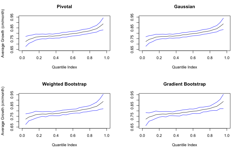
As we can see in Figure 1, the confidence bands generated are roughly similar. Note that the point estimates are the same for all the methods.

We can compare the computation times of each of the approximations using the command Sys.time. Additionally, we compare the p-values generated by each of the four inference methods. Note that computation times may vary widely depending on the machine in use. However, the relative computation times will be approximately constant across different machines. The computation times in the table below were obtained on a computer with two eight-core 2.6 GHz processors (note: npqr does not make use of parallel computing).

pval.dimnames <- vector("list", 2)pval.dimnames[[1]] <- c("Pivotal", "Gaussian", "Weighted Bootstrap","Gradient Bootstrap")pval.dimnames[[2]] <- c("H0: Growth Rate <= 0", "H0: Growth Rate >= 0","H0: Growth Rate = 0", "Computation Minutes")pvals <- matrix(NA, nrow = 4, ncol = 4, dimnames = pval.dimnames)pvals[1,] <- c(round(piv.bsp$pvalues, digits = 4), round(piv.time, digits = 0))pvals[2,] <- c(round(gaus.bsp$pvalues, digits = 4), round(gaus.time, digits = 0))pvals[3,] <- c(round(wboot.bsp$pvalues, digits = 4), round(wboot.time, digits = 0))pvals[4,] <- c(round(gboot.bsp$pvalues, digits = 4), round(gboot.time, digits = 0))print(pvals)

These commands generate the output:

	H0: Growth	H0: Growth	H0: Growth	Computation
	Rate <= 0	Rate >= 0	Rate = 0	Minutes
Pivotal	0	1	0.0237	0.9
Gaussian	0	1	0.0234	0.6
Weighted Bootstrap	0	1	0.0221	30
Gradient Bootstrap	0	1	0.0221	346

As expected, we reject at the 5% level the null hypothesis that the growth rate is negative and the null hypothesis that the growth rate is equal to zero in all cases, and we fail to reject the null hypothesis that the growth rate is positive in all cases. For the one-sided tests, the relevant null hypothesis is that the average growth rate is less than or equal to zero (greater than or equal to zero) at all the quantile indices in taus. For the two-sided test, the relevant null hypothesis is that the average growth rate is equal to zero at all the quantile indices in taus. Additionally, note that the pivotal and Gaussian methods are substantially faster than the two bootstrap methods.

Comparison of series bases

Another option is to take advantage of the variety of bases available in the quantreg.nonpar package. Here, we consider three bases: the B-spline basis used in the analysis above, an orthogonal polynomial basis of degree 12, and a Fourier basis with 9 basis functions and a period of 200 months. We compare the estimates of the average quantile derivative function generated by using each of these bases. We construct the orthogonal polynomial basis and the Fourier basis with the commands:

basis.poly <- poly(cage, degree = 12)basis.four <- create.fourier.basis(rangeval = range(data$cage), nbasis = 9,                     period = 200)

In this section, we focus on the pivotal method for inference. We run npqr for the orthogonal polynomial basis and the Fourier basis, mimicking the analysis run above for the B-spline basis.

piv.poly <- update(piv.bsp, basis = basis.poly)piv.four <- update(piv.bsp, basis = basis.four)

Figure 2: Comparison of Series Bases for Growth Rate: point estimates and 95% uniform confidence bands for the average derivative of the conditional quantile function of height with respect to age based on B-spline, polynomial, and Fourier series approximations.

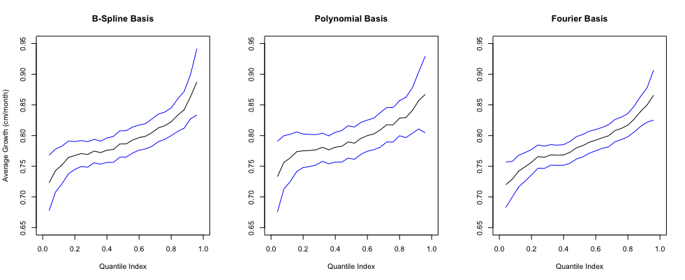
Similar to Section Comparison of the inference processes, we plot the point estimates with their uniform 95% confidence bands for each basis. Figure 2 shows that, given the parameters of the chosen bases, the type of basis does not have an important impact on the estimation and inference on the growth rate charts. A table containing the p-values associated with the hypothesis tests for each basis are generated by the following code:

pval2.dimnames <- vector("list", 2)pval2.dimnames[[1]] <- c("B-spline", "Polynomial", "Fourier")pval2.dimnames[[2]] <- c("H0: Growth Rate <= 0", "H0: Growth Rate >= 0","H0: Growth Rate = 0")pvals2 <- matrix(NA, nrow = 3, ncol = 3, dimnames = pval2.dimnames)pvals2[1,] <- round(piv.bsp$pvalues, digits = 4)pvals2[2,] <- round(piv.poly$pvalues, digits = 4)pvals2[3,] <- round(piv.four$pvalues, digits = 4)print(pvals2)

These commands yield:

	H0: Growth	H0: Growth	H0: Growth
	Rate <= 0	Rate >= 0	Rate = 0
B-Spline	0	1	0.0239
Polynomial	0	1	0.0334
Fourier	0	1	0.0386

For all bases, the tests’ conclusions are identical: at the 5% level, we reject the null hypothesis that the average growth rate is negative, fail to reject the null hypothesis that the average growth rate is positive, and reject the null hypothesis that the average growth rate is equal to zero.

Confidence intervals and standard errors

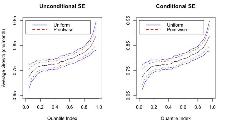
Now, we illustrate two additional options available to the user. First, to perform inference pointwise over a region of covariate values and/or quantile indices instead of uniformly, and second, to estimate the standard errors conditional on the values of the covariate $W$ in the sample. When inference is uniform, the test statistic used in construction of the confidence interval is the maximal t-statistic across all covariate values and quantile indices in the region of interest, whereas pointwise inference uses the t-statistic at each covariate value and quantile index. When standard errors are estimated unconditionally, a correction term is used to account for the fact that the empirical distribution of $W$ is an estimator of the distribution of $W$. The option to estimate standard errors conditionally or unconditionally is not available for the bootstrap methods. The inference based on these methods is always unconditional.

We will use only the pivotal method with a B-spline basis for this illustration. First, we run npqr for each combination of options mentioned above:

piv.bsp <- npqr(formula = form.par, basis = basis.bsp, var = "cage", taus = taus,B = B, nderivs = 1, average = 1, alpha = alpha, process = "pivotal",uniform = T, se = "unconditional", printOutput = F)piv.bsp.cond <- update(piv.bsp, se = "conditional")piv.bsp.point <- update(piv.bsp,  uniform = F, se = "unconditional")piv.bsp.point.cond <- update(piv.bsp,  uniform = F, se = "conditional")

We obtain Figure 3 using the graphing techniques described in Sections Comparison of the inference processes and Comparison of series bases. As is visible in this figure, usage of conditional standard errors changes the confidence bands only minimally in our example. As expected, the pointwise confidence bands are narrower than the uniform confidence bands.

Figure 3: Comparison of Pointwise vs Uniform and Conditional vs Unconditional Inference for Growth Rate: 95% uniform and pointwise confidence bands for the average derivative of the conditional quantile function of height with respect to age based on B-spline series approximation. The left panel uses unconditional standard errors in the construction of the bands. The right panel uses conditional standard errors.

We can also compare how much of the differences (or lack thereof) in the confidence bands are driven by differences in the standard errors versus the test statistics. Here, we compare the estimated standard errors at the median for conditional versus unconditional inference:

piv.bsp.med <- npqr(formula = form.par, basis = basis.bsp, var = "cage", taus = 0.5,B = B, nderivs = 1, average = 1, alpha = alpha, process = "pivotal", uniform=T,se = "unconditional", printOutput = F)piv.bsp.cond.med <- update(piv.bsp.med, se = "conditional")stderr.dimnames <- vector("list",2)stderr.dimnames[[1]] <- c("Unconditional", "Conditional")stderr.dimnames[[2]] <- c("Standard Error")stderr <- matrix(NA, nrow = 2, ncol = 1, dimnames = stderr.dimnames)stderr[1,] <- piv.bsp.med$std.error[1]stderr[2,] <- piv.bsp.cond.med$std.error[1]print(stderr)

These commands yield the output:

	Standard Error
Unconditional	0.008104
Conditional	0.007663

Finally, we compare p-values generated by each of the option choices:

pval3.dimnames <- vector("list", 2)pval3.dimnames[[1]] <- c("Uniform, Unconditional", "Uniform, Conditional","Pointwise, Unconditional", "Pointwise, Conditional")pval3.dimnames[[2]] <- c("H0: Growth Rate <= 0", "H0: Growth Rate >= 0","H0: Growth Rate = 0")pvals3 <- matrix(NA, nrow = 4, ncol = 3, dimnames = pval3.dimnames)pvals3[1,] <- round(piv.bsp$pvalues, digits = 4)pvals3[2,] <- round(piv.bsp.cond$pvalues, digits = 4)pvals3[3,] <- round(piv.bsp.point$pvalues, digits = 4)pvals3[4,] <- round(piv.bsp.point.cond$pvalues, digits = 4)print(pvals3)

	H0: Growth	H0: Growth	H0: Growth
	Rate <= 0	Rate >= 0	Rate = 0
Uniform, Unconditional	0	1	0.0239
Uniform, Conditional	0	1	0.0243
Pointwise, Unconditional	0	1	0.0267
Pointwise, Conditional	0	1	0.0222

In this example, where the sample size is large, about 38,000 observations, conditional versus unconditional standard errors and uniform versus pointwise inference have little impact on the estimated p-values.

Estimation and uniform inference on linear functionals

Finally, we illustrate how to estimate and make uniform inference on linear functionals of the conditional quantile function over a region of covariate values and quantile indices. These functionals include the function itself and derivatives with respect to the covariate of interest. The quantreg.nonpar package is able to perform estimation and inference on the conditional quantile function, its first derivative, and its second derivative over a region of covariate values and/or quantile indices. We also illustrate how to report the estimates using three dimensional plots.

First, we consider the first and second derivatives of the conditional quantile function. In the application they correspond to the growth rate and growth acceleration of height with respect to age as a function of age (from 0 to 59 months) and the quantile index. To do so, we use the output of npqr called var.unique, which contains a vector with all the distinct values of the covariate of interest (cage here). To generate this output, we estimate the first and second derivatives of the conditional quantile function using a B-spline series approximation over the covariate values in var.unique and the quantile indices in taus:

piv.bsp.firstderiv <- npqr(formula = form.par, basis = basis.bsp, var = "cage",taus = taus, nderivs = 1, average = 0, print.taus = print.taus, B = B,process = "none", printOutput = F)piv.bsp.secondderiv <- update(piv.bsp.firstderiv, nderivs = 2)

Next, we generate vectors containing the region of covariate values and quantile indices of interest:

xsurf1 <- as.vector(piv.bsp.firstderiv$taus)ysurf1 <- as.vector(piv.bsp.firstderiv$var.unique)zsurf1 <- t(piv.bsp.firstderiv$point.est)xsurf2 <- as.vector(piv.bsp.secondderiv$taus)ysurf2 <- as.vector(piv.bsp.secondderiv$var.unique)zsurf2 <- t(piv.bsp.secondderiv$point.est)

Finally, we create the three dimensional plots for:

$$\left(\tau,w\right)\mapsto\partial^{k}g\left(\tau,w\right)/\partial w^{k},\ \ \left(\tau,w\right)\in I,$$

where $k\in\{1,2\}$, and $I$ is the region of interest.

par(mfrow = c(1, 2))persp(xsurf1, ysurf1, zsurf1, xlab = "Quantile Index", ylab = "Age (months)",zlab = "Growth Rate", ticktype = "detailed", phi = 30, theta = 120, d = 5,col = "green", shade = 0.75, main = "Growth Rate (B-splines)")persp(xsurf2, ysurf2, zsurf2, xlab = "Quantile Index", ylab = "Age (months)",zlab = "Growth Acceleration", ticktype = "detailed", phi = 30, theta = 120,d = 5, col = "green", shade = 0.75, main = "Growth Acceleration (B-splines)")

Figure 4: Growth Rate and Acceleration: estimates of the first and second derivatives of the conditional quantile function of height with respect to age.

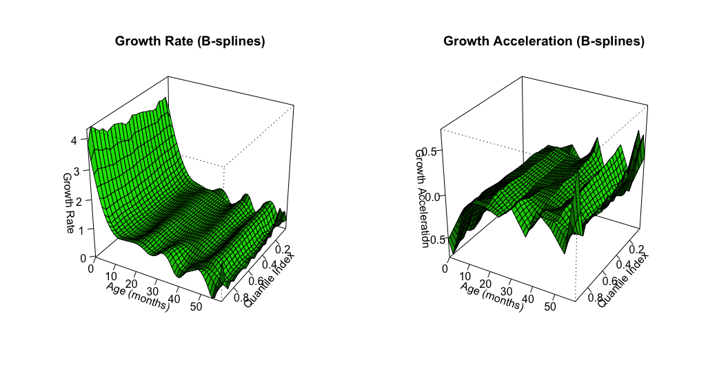
These commands produce Figure 4. Here, we see that the growth rate is positive at all ages and quantile indices. The growth rate decreases in the first few months of life and stabilizes afterwards, which can also be seen in the graph of growth acceleration. Growth acceleration is negative at young ages but stabilizes around zero at about 15 months. Both growth rate and growth acceleration are relatively homogeneous across quantiles at all ages. Saved in piv.bsp.firstderiv$pvalues and piv.bsp.secondderiv$pvalues are the p-values from hypothesis tests to determine whether the first and second derivatives, respectively, are negative, positive, and equal to zero uniformly over the region of ages and quantile indices:

Order of	H0: Growth	H0: Growth	H0: Growth
Derivative	Rate <= 0	Rate >= 0	Rate = 0
First Derivative	0	1	0.042
Second Derivative	1	0	0.061

Thus, we reject at the 5% level the null hypotheses that growth rate is negative, that growth rate is equal to zero, and that growth acceleration is positive over all the first five years of the children’s lives at all the quantiles of interest. We come close to rejecting at the 5% level the null hypothesis that growth acceleration is equal to zero over all the first five years of the children’s lives at all the quantiles of interest.

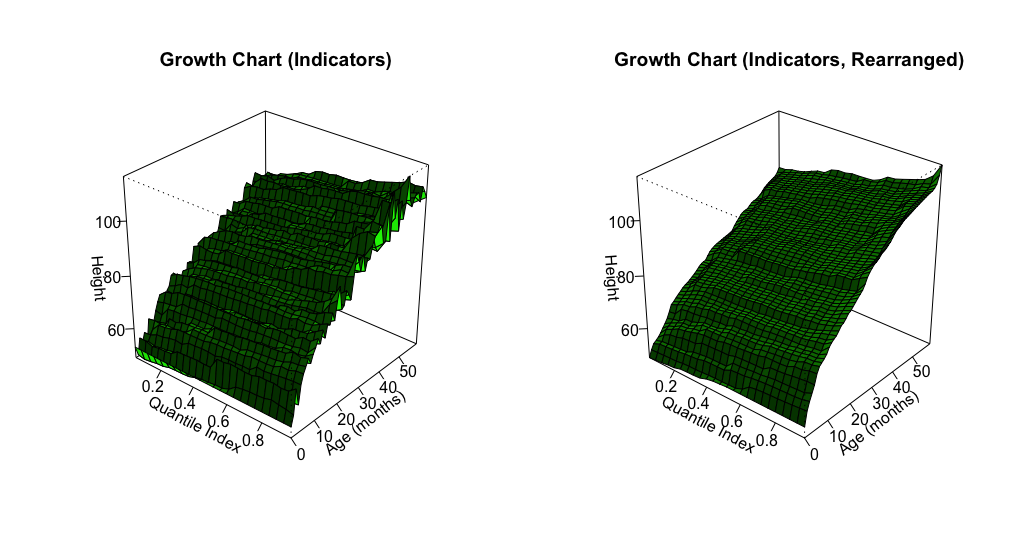
Similarly, we estimate the conditional quantile function over a region of covariate values and quantile indices, which corresponds to a growth chart in our application. Here, we use a fully saturated indicator basis for the series approximation to the nonparametric part of the model. We also compare the original estimates of the resulting growth chart to rearranged estimates that impose that the conditional quantile function of height is monotone in age and the quantile index. In this example, the conditional quantile function estimated using all data is nearly monotone without rearrangement. To illustrate the power of rearrangement when estimates are not monotone, we use a subset of the data containing the first 1,000 observations:

data.subset <- data[1:1000,]detach(data)attach(data.subset)

Now, we create the fully saturated indicator basis for cage:

faccage <- factor(cage)

To perform estimation using this basis, we input faccage for basis:

piv.fac.fun <- npqr(formula = form.par, basis = faccage, var = "cage", taus = taus,print.taus = print.taus, B = B, nderivs = 0, average = 0, alpha = alpha,process = "none", rearrange = F, rearrange.vars="both", se = "conditional",printOutput = F, method = "fn")

We also obtain the rearranged estimates with respect to age and the quantile index using the options of the command npqr. Note that we input "both" for rearrange.vars. This option performs rearrangement over quantile indices and age. Other allowable options are "quantile" (for monotonization over quantile indices only) and "var" (for monotonization over the variable of interest only).

piv.fac.fun.re <- update(piv.fac.fun, rearrange.vars = "both")

Now, we construct three dimensional plots for the estimates of the conditional quantile function:

$$\left(\tau,w\right)\mapsto Q_{Y\mid X}\left(\tau\mid x\right)=g\left(\tau,w\right)+v^{\prime}\gamma\left(\tau\right),\ \ \left(\tau,w\right)\in I,$$

where $v$ are evaluated at the sample mean for cardinal variables (mbmi, breastfeeding, mage, medu, and edupartner) and the sample mode for unordered factor variables (faccsex, facctwin, faccbirthorder, facmunemployed, facmreligion, facmresidence, facwealth, facelectricity, facradio,
factelevision, facrefrigerator, facbicycle, facmotorcycle, and faccar).

xsurf <- as.vector(piv.fac.fun$taus)ysurf <- as.vector(piv.fac.fun$var.unique)zsurf.fac <- t(piv.fac.fun$point.est)zsurf.fac.re <- t(piv.fac.fun.re$point.est)par(mfrow = c(1, 2))persp(xsurf, ysurf, zsurf.fac, xlab = "Quantile Index", ylab = "Age (months)",zlab = "Height", ticktype = "detailed", phi = 30, theta = 40, d = 5,col = "green", shade = 0.75, main = "Growth Chart (Indicators)")persp(xsurf, ysurf, zsurf.fac.re, xlab = "Quantile Index", ylab = "Age (months)",zlab = "Height", ticktype = "detailed", phi = 30, theta = 40, d = 5,col = "green", shade = 0.75, main = "Growth Chart (Indicators, Rearranged)")

Figure 5 shows that the rearrangement fixes the non-monotonic areas of the original estimates.

Figure 5: Growth Chart, with and without Rearrangement: estimates of the conditional quantile function of height based on a fully saturated indicator approximation with respect to age.

Conclusion

In this paper we introduced the R package quantreg.nonpar, which implements the methods of Belloni et al. (2011) to estimate and make inference on partially linear quantile models. The package allows the user to obtain point estimates of the conditional quantile function and its derivatives based on a nonparametric series QR approximation. Using pivotal, gradient bootstrap, Gaussian, and a weighted bootstrap methods, the user is also able to obtain pointwise and uniform confidence intervals. We apply the package to a dataset containing information on child malnutrition in India, illustrating the ability of quantreg.nonpar to generate point estimates and confidence intervals, as well as output that allows for easy visualization of the computed values. We also illustrate the ability of the package to monotonize estimates by the variable of interest and by quantile index.

Michael Lipsitz
Boston University
Department of Economics
USA
lipsitzm@bu.edu

Alexandre Belloni
Duke University
Fuqua School of Business
USA
abn5@duke.edu

Victor Chernozhukov
MIT
Department of Economics
USA
vchern@mit.edu

Iván Fernández-Val
Boston University
Department of Economics
USA
ivanf@bu.edu

References

- Belloni et al. (2011) A. Belloni, V. Chernozhukov, D. Chetverikov, and I. Fernandez-Val. Conditional Quantile Processes based on Series or Many Regressors. ArXiv e-prints, May 2011.
- Charlier et al. (2015) I. Charlier, D. Paindaveine, and J. Saracco. QuantifQuantile: Estimation of Conditional Quantiles using Optimal Quantization, 2015. URL https://CRAN.R-project.org/package=QuantifQuantile. R package version 2.2.
- Chernozhukov et al. (2009) V. Chernozhukov, I. Fernández-Val, and A. Galichon. Improving point and interval estimators of monotone functions by rearrangement. Biometrika, 96(3):559–575, 2009.
- Chernozhukov et al. (2010) V. Chernozhukov, I. Fernández-Val, and A. Galichon. Quantile and probability curves without crossing. Econometrica, 78(3):1093–1125, 2010.
- Koenker (2011) R. Koenker. Additive models for quantile regression: Model selection and confidence bandaids. Braz. J. Probab. Stat., 25(3):239–262, 11 2011. doi: 10.1214/10-BJPS131. URL http://dx.doi.org/10.1214/10-BJPS131.
- Koenker (2016) R. Koenker. quantreg: Quantile Regression, 2016. URL https://CRAN.R-project.org/package=quantreg. R package version 5.21.
- Koenker and Basset (1978) R. Koenker and G. Basset. Regression quantiles. Econometrica, 46(1):33–50, 1978.
- Muggeo et al. (2013) V. Muggeo, M. Sciandra, A. Tomasello, and S. Calvo. Estimating growth charts via nonparametric quantile regression: a practical framework with application in ecology. Environmental and Ecological Statistics, 20:519–531, 2013.
- Ramsay et al. (2014) J. O. Ramsay, H. Wickham, S. Graves, and G. Hooker. fda: Functional Data Analysis, 2014. URL https://CRAN.R-project.org/package=fda. R package version 2.4.4.