APPROXIMATE EIGENVALUE DISTRIBUTION OF A CYLINDRICALLY ISOTROPIC NOISE SAMPLE COVARIANCE MATRIX

Abstract

The statistical behavior of the eigenvalues of the sample covariance matrix (SCM) plays a key role in determining the performance of adaptive beamformers (ABF) in presence of noise. This paper presents a method to compute the approximate eigenvalue density function (EDF) for the SCM of a cylindrically isotropic noise field when only a finite number of shapshots are available. The EDF of the ensemble covariance matrix (ECM) is modeled as an atomic density with many fewer atoms than the SCM size. The model results in substantial computational savings over more direct methods of computing the EDF. The approximate EDF obtained from this method agrees closely with histograms of eigenvalues obtained from simulation.

Index Terms—  Random Matrix Theory, Cylindrically Isotropic Noise, Sample Covariance Matrix, Polynomial Method

1 Introduction

In array processing, adaptive beamformers (ABF) rely on the knowledge of the spatial covariance matrix of the data [1]. In most applications the ensemble covariance matrix (ECM) is not known a priori, thus it must be estimated from measurements. A common technique for estimating the ECM is to compute the sample covariance matrix (SCM).

A spatially white background noise is a common assumption in analyzing the performance of ABFs in presence of noise. In practice however, a spatially correlated noise field may exist in the environment. In a shallow underwater acoustic channel, the correlated noise is generally modeled as cylindrically isotropic field [2]. The noise model developed in [3] simplifies to cylindrically isotropic noise for a horizontal linear array at a constant depth.

Assuming a uniform linear array placed on the plane of symmetry of the noise field, the entries of the ECM ($\boldsymbol{\Sigma}_{X}$) for the cylindrically isotropic noise field are given by

$$[\boldsymbol{\Sigma}_{X}]_{pq}=J_{0}(2\pi\zeta|p-q|),$$ (1)

where $J_{0}()$ is the zeroth order Bessel function of the first kind and $\zeta$ is the ratio of the sensor spacing to wavelength. The statistical behavior of the eigenvalues and eigenvectors of the SCM in the presence of noise plays a crucial role in the performance of ABFs. Thus, understanding the distribution of the eigenvalues of the noise SCM is important for ABFs.

Traditionally the replacement of the ECM by the SCM in ABFs was justified by the asymptotic convergence of the SCM to the ECM. However, in practice the SCM has to be estimated from a finite number of snapshots. The number of snapshots ($L$) available is usually on the order of the number of sensors ($N$) in the array. In practice and in simulations it has been observed that the performance of the ABF depends on the ratio $N/L$ [1].

Random Matrix Theory (RMT) offers an attractive framework to understand the behaviors of SCMs. RMT has results for the eigenstructure of SCMs as the number of rows $N$ and columns $L$ of the data matrix go to infinity while $N/L\rightarrow c$. The resulting distributions are therefore characterized by the same ratio that appears in ABF performance analysis. Although RMT results are for the limiting case of infinitely large matrices, they are frequently accurate for modest data sizes. This makes the RMT approach well suited for analyzing the eigenvalue distribution of the SCM.

The Polynomial Method (PM) is an RMT technique for calculating the asymptotic eigenvalue distribution of a class of ‘algebraic’ random matrices [4]. The Stieltjes transform of the EDF of algebraic random matrices satisfies a polynomial equation. The PM is based on a transform representation of a random matrix. Conceptually, this is similar to the Laplace transform used to represent scalar random variables by polynomial moment generating functions. Both techniques are based on a one-to-one correspondence between probability density functions (PDFs) and polynomials. The Laplace transform represents the PDFs of a scalar random variable as a univariate polynomials, i.e., moment generating functions. The PM requires several additional layers in its transform representation whose details are well beyond the limited scope of the present paper. The central concept is that the PDF for the eigenvalues of a random matrix is represented by a bivariate polynomial. A set of deterministic and stochastic operations on random matrices are mapped to operations on the bivariate polynomials. The polynomial representations are thus manipulated in the manner corresponding to the desired operations on the random matrices. Finally, the polynomial representation is transformed back to the EDF of the desired output random matrix. The bivariate polynomial manipulations corresponding to common matrix operations can be quite complicated, but fortunately the toolbox RMTool is available to handle the symbolic algebra [5].

This paper presents a method to predict an approximate EDF for the SCM of a cylindrically isotropic noise field. The technique presented here is similar in spirit to the results presented in [6], but it differs in two important ways. First, this paper focuses on cylindrically isotropic noise rather than the spherically isotropic noise in [6]. Second, this paper exploits the PM and its RMTool toolbox rather than working directly with the Stieltjes transform as in [6].

The next section describes the method of applying the PM to obtain an approximate EDF of the noise SCM. Sec. 3 illustrates the application of this technique for a particular array size. Finally, Sec. 4 provides a short discussion of the results.

2 Method

This section describes a technique to compute an approximate EDF for the SCM of cylindrically isotropic noise observed by a uniform linear array (ULA). The technique exploits properties of free multiplicative convolution [4] to approximate the eigenvalue density of an $N\times N$ SCM by replacing the EDF of the ECM by an atomic density (PDF containing only Dirac delta functions) with fewer than $N$ atoms. The PM computes a numerical approximation to the SCM EDF using this lower order atomic density.

Let $\boldsymbol{\Sigma}_{X}$ be the ECM for the cylindrically isotropic noise measured at the $N$-element ULA. The entries of this matrix are given by (1). The eigenvalues of $\boldsymbol{\Sigma}_{X}$ are $\gamma_{1}\geq\gamma_{2}\geq\ldots\gamma_{N}\geq 0$. The data matrix ${\bf X}$ is an $N\times L$ matrix of complex phasors representing the $L$ temporally independent but spatially correlated snapshots observed on the array after demodulating to baseband. These snapshots can be modeled as ${\bf X}=\boldsymbol{\Sigma}_{X}^{1/2}{\bf\mathcal{G}}$, where ${\bf\mathcal{G}}$ is an $N\times L$ matrix of independent, identically distributed proper complex Gaussian random variables with zero mean and unit variance. This model guarantees that the SCM converges to the desired ECM, i.e. $E\{(1/L){\bf X}{\bf X}^{H}\}=\boldsymbol{\Sigma}_{X}$.

The SCM is computed from the data matrix ${\mathbf{X}}$ as

$${\bf S}_{X}=(1/L){\mathbf{X}}{\mathbf{X}}^{H}=(1/L)\boldsymbol{\Sigma}_{X}^{1/2}({\bf\mathcal{G}}{\bf\mathcal{G}}^{H})\boldsymbol{\Sigma}_{X}^{1/2}.$$ (2)

The eigenvalues of ${\bf S}_{X}$ are $g_{1}\geq g_{2}\geq\ldots g_{N}$. The SCM of ${\bf\mathcal{G}}$ is a Wishart matrix ${\bf W}(c)=(1/L){\bf\mathcal{G}}{\bf\mathcal{G}}^{H}$ where $c=N/L$. Thus the SCM in (2) can be expressed as ${\bf S}_{X}=\boldsymbol{\Sigma}_{X}^{1/2}{\bf W}(c)\boldsymbol{\Sigma}_{X}^{1/2n}$. This matrix has the same eigenvalues as the product $\boldsymbol{\Sigma}_{X}$${\bf W}(c)$. The Wishart matrix is an algebraic matrix [4, Remark 5.15] with an EDF given by the Marčenko-Pastur (MP) density $f_{MP(c)}{}(x)$ parameterized by $c$ [7]. If $\boldsymbol{\Sigma}_{X}$ is an algebraic matrix, then the product is also an algebraic matrix [4, Theorem 5.19]. Thus, if $\boldsymbol{\Sigma}_{X}$ can be modeled as an algebraic matrix, the PM provides a straightforward way to compute the eigenvalue density for $\boldsymbol{\Sigma}_{X}{\bf W}(c){}$, or equivalently, the EDF for the SCM.

The simplest way to create an algebraic density for $\boldsymbol{\Sigma}_{X}$ is to construct an atomic density with all $N$ eigenvalues of $\boldsymbol{\Sigma}_{X}$, each with mass $1/N$. All matrices with atomic eigenvalue densities fall within the class of algebraic random matrices [4, Example 3.6]. The polynomial representation of the SCM ${\bf S}_{X}$ ($L_{mz}^{{\bf S}_{X}}$) can be found directly from the polynomials representing $\boldsymbol{\Sigma}_{X}$ ($L_{mz}^{\boldsymbol{\Sigma}_{X}}$) and the Wishart matrix ${\bf W}(c)$ ($L_{mz}^{{\bf W}(c)}$) using the Multiply Wishart operation in the PM [4, Table 7]. The dependence of the SCM eigenvalues on the number of snapshots enters through the parameterization of $L_{mz}^{{\bf W}(c)}$. An inverse operation is performed on $L_{mz}^{{\bf S}_{X}}$ to extract the desired density $f^{{\bf S}_{X}}(x)$ on the support region of interest [5].

The drawback of this approach is that the degree in $m$ of the polynomial $L_{mz}^{{\bf S}_{X}}$ grows as $\mathcal{O}(N)$. Moreover, the free multiplicative convolution (FMC) describing $\boldsymbol{\Sigma}_{X}$${\bf W}(c)$ replaces each impulse in the atomic EDF of $\boldsymbol{\Sigma}_{X}$ with some non-linearly convolved version of the MP density, i.e., $\hat{f}(x)$, to produce the continuous eigenvalue density function for ${\bf S}_{X}$. The ensemble eigenvalues whose separation is much less than the support region the density $\hat{f}(x){}$ will be smeared together resulting into single continuous density. This suggests that the eigenvalue density of ${\bf S}_{X}$ can be modeled using many fewer than $N$ atoms for the density of $\boldsymbol{\Sigma}_{X}$ by intelligently exploiting the smearing that results when multiplying $\boldsymbol{\Sigma}_{X}$ by a Wishart matrix. As a result, the EDF $f^{\boldsymbol{\Sigma}_{X}}(x)$ generated by using all $N$ atoms from $\boldsymbol{\Sigma}_{X}$ can be replaced by a modified EDF $\tilde{f}^{\boldsymbol{\Sigma}_{X}}(x)$ with many fewer atoms, resulting in a much lower order polynomial $L_{mz}^{{\bf S}_{X}}$ substantially reducing computational time.

Designing the reduced order model relies on properties of the covariance matrix $\boldsymbol{\Sigma}_{X}{}$ for cylindrically isotropic noise. The covariance matrix is a Hermitian Toeplitz matrix whose entries are samples of $J_{0}(\alpha n)$. The eigenvalues of such a matrix are asymptotically equally distributed as the samples of the Fourier transform of the entries of the first row of $\boldsymbol{\Sigma}_{X}$. For cylindrically isotropic noise, the first row is $J_{0}(\alpha n)$ [8, 9] and the Fourier transform is equal to $F(\omega)=2/\sqrt{\alpha^{2}-\omega^{2}}$ for $|\omega|<\alpha$. The form of this Fourier transform implies that most of eigenvalues will be very close to $2/\alpha$,thus very close together relative to the width of the resulting MP density. Only a small subset of eigenvalues will be sufficiently spaced to remain distinct after smearing by the MP PDF in the nonlinear FMC. Fig. 1 shows the eigenvalues of $\boldsymbol{\Sigma}_{X}$ for N = 51, where the eigenvalues are plotted on the horizontal axis against their index on the vertical. This behavior is very similar to what is known as a spiked covariance model in RMT.

The SCM eigenvalue behavior for a spiked covariance model is described in [10]. This model assumes that the data matrix consists of a low rank perturbation in a unit power white noise background. In the event that the white noise background is not unit power, it is straightforward to scale the problem by the eigenvalue $\gamma_{N}$ representing the background power. Assuming $\gamma_{N}=1$, the $N_{low}$ ensemble eigenvalues between $(1+\sqrt{c})$ and 1 will produce $N_{low}$ SCM eigenvalues $g_{N-N_{low}+1},\ldots,g_{N_{low}}$ distributed nearly indistinguishably than if there had been a single atom at $1$ with mass $N_{low}/N$ [10]. This suggests that all ensemble eigenvalues $\gamma_{i}\leq(1+\sqrt{c})$ can be collapsed into a single atom at $\gamma_{N}=1$ with mass $N_{low}/N$ without significant impact on the SCM eigenvalue distribution. This atom will be replaced by the non-linearly convolved version of MP density $\hat{f}(x){}$, in the EDF of ${\bf S}_{X}$. The eigenvalues with $\gamma_{i}>(1+\sqrt{c})$ will behave as distinct atoms in principle. However, many of these atoms are also very closely spaced relative to the width of support width of $\hat{f}(x)$ and will also be smeared together nearly indistinguishably in the density for ${\bf S}_{X}$. Consequently, these atoms are also collapsed into a single atom at $\gamma_{mid}=((1+\sqrt{c})+(1+\sqrt{c})^{2})/2$. Finally the eigenvalues above $(1+\sqrt{c})^{2}$ maintain their identity as distinct atoms.

To define the model precisely, let $\Gamma_{dist}=\{\gamma_{i}|\gamma_{i}>(1+\sqrt{c})^{2}\}$ be a set of atoms expected to remain distinct even after FMC. The number of eigenvalues in different ranges are given by $N_{mid}=|\{\gamma_{i}|(1+\sqrt{c})<\gamma_{i}<(1+\sqrt{c})^{2}\}|$ and $N_{low}=|\{\gamma_{i}|1\leq\gamma_{i}\leq(1+\sqrt{c})\}|$ where $|\cdot|$ indicates the cardinality of the set. Then the modified EDF for $\boldsymbol{\Sigma}_{X}$ is

$$\tilde{f}^{\boldsymbol{\Sigma}_{X}{}}(x) =\frac{1}{N}\sum\limits_{\gamma_{i}\in\Gamma_{dist}}\delta(x-\gamma_{i})+$$

$$\frac{N_{mid}}{N}\delta(x-\gamma_{mid})+\frac{N_{low}}{N}\delta(x-\gamma_{N})$$ (3)

The SCM eigenvalue density $f^{{\bf S}_{X}}(x)$ can be computed using (3) and the multiplication by Wishart properly as described earlier.

This approach results in a much lower order polynomial $L_{mz}^{{\bf S}_{X}}$ to represent ${\bf S}_{X}$. For the example in Fig. 1, this approach reduces the atomic distribution from $N=51$ to a mere $5$ atoms. The computation required in solving for the roots of the polynomial $L_{mz}^{{\bf S}_{X}}$ is of the order $\mathcal{O}(N^{3})$ [11]. Hence the lowered polynomial degree results in substantial savings in computational requirement.

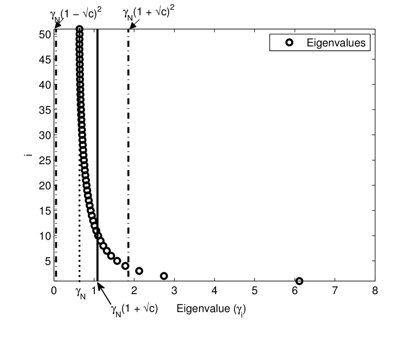
Fig. 1: Ensemble eigenvalues (circles) of $\boldsymbol{\Sigma}_{X}$ computed for the case of $N=51$ and $c=0.25$. The support set of Marčenko-Pastur distribution is denoted by dashed lines and the threshold value is denoted by the solid line.

3 Simulation Results

This section compares the SCM eigenvalue density predicted by the model described in Sec. 2 with histograms obtained through Monte Carlo simulations of cylindrically isotropic noise measured at a horizontal ULA with $N=51$ sensors at $\lambda/2$ spacing. The approximate EDFs obtained for the SCM are compared with simulation results for different numbers of snapshots to verify the accuracy of the technique. Fig. 2 compares the EDF predicted by the method in Sec. 3 with a histogram obtained from 5000 Monte Carlo simulations.

Fig. 1 shows the ensemble eigenvalues (circles) for $\boldsymbol{\Sigma}_{X}$. Note that most of the eigenvalues are clustered around the smallest eigenvalue $\gamma_{N}=2/\pi=0.6366$ and a few eigenvalues are distinctly larger than the rest. As mentioned in the Sec. 2, $\boldsymbol{\Sigma}_{X}$ can be viewed as a spiked covariance matrix, most of whose eigenvalues are $\gamma_{N}=0.6366$. Note that because the smallest eigenvalue is not one as in the canonical spiked covariance model, the threshold and support regions for the model must all be scaled by $\gamma_{N}$ when determining the atomic distribution. Thus, the two dashed lines in Fig. 2 indicate the upper and the lower limit of the Marčenko-Pastur density scaled by $\gamma_{N}$, and the solid line indicates the scaled threshold value. Note that there are at least three dominant ensemble eigenvalues, one well separated at around $\gamma_{1}=6.11$ and two slightly separated around $\gamma_{2}=2.74$ and $\gamma_{3}=2.12$.

Fig. 2 shows a comparison of the approximate EDF for the SCM and the histograms. The blue line indicates the approximate EDF computed using the PM, while the red circles indicate the histogram from the simulation. The four panels correspond to $c=\{0.25,0.5,1,1.5\}$ from top to bottom, respectively. The choice of values for $c$ covers a range of sensor to snapshot ratios that describe many practical scenarios.

In all four cases, there is close agreement between the EDF and the simulation histograms, suggesting that this method for approximating the EDF of the cylindrically isotropic noise SCM is accurate. Note that for the cases with $c>1$, ${\bf S}_{X}$ is singular thus, the eigenvalue density also includes an impulse of area $(1-1/c)$ at $x=0$ that is not shown on these figures.

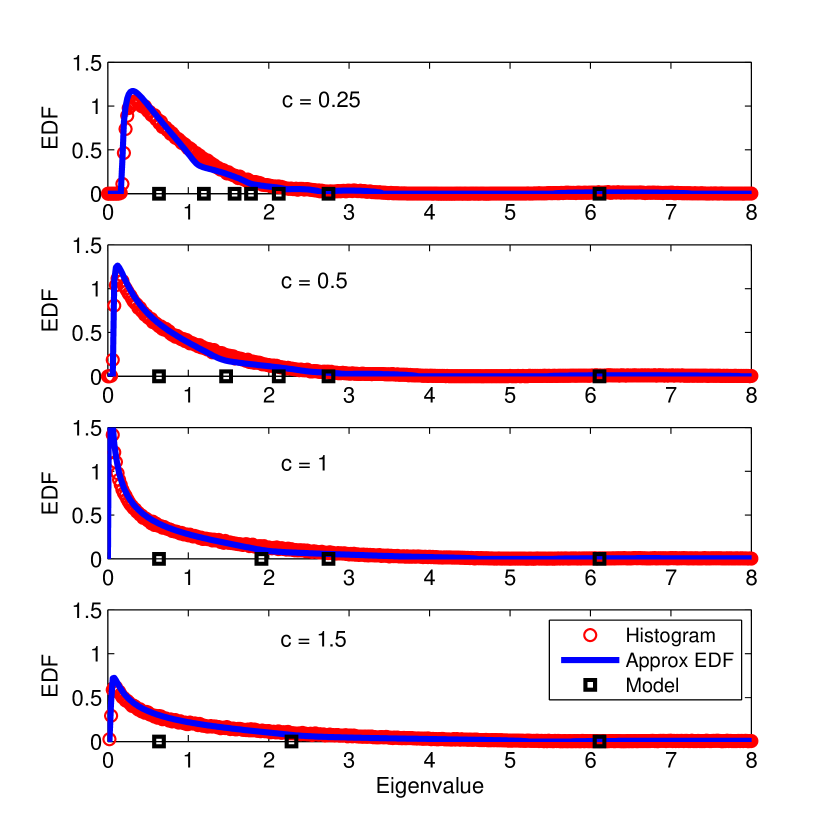
Fig. 2: Comparison of approximate EDF (solid blue) with histogram of eigenvalues (red circles) observed from 5000 Monte Carlo simulations of N = 51 element horizontal uniform linear array. The location of atoms for the EDF in (3) are shown as black squares in each panel. The four panels shows different scenario from snapshot rich case at the top ($L=204,c=0.25$) to snapshot deficient case at the bottom ($L=34,c=1.5$).

4 Discussion and Conclusion

The simulation results in Fig. 2 confirm that the approximate EDF computed from the method in Sec. 2 gives a good approximation of the histogram of the eigenvalues obtained from the simulation.

In practice this algorithm is limited by the symbolic computation of the roots of $L_{mz}$ for the Stieltjes transform $m(z)$ for the SCM [5]. As noted in Sec. 2, the degree of the polynomial $L_{mz}$ in $m$ grows with the number of atoms in the model density function (3). From (3) it is evident that the eigenvalues below $(1+\sqrt{c})^{2}$ always contribute two atoms. But the eigenvalues above $(1+\sqrt{c})^{2}$ contribute as distinct atoms. The number of eigenvalues modeled as distinct atoms depends on the choice of $c$ and $N$. As the order of $L_{mz}^{{\bf S}_{X}}$ grows, the number of roots to be solved for also grows.

This model can be combined with signal models to produce more accurate estimates of ABF performance for bearing estimation in shallow water where the background noise is often cylindrically isotropic. Additionally, as discussed in [6], understanding the nature of the isotropic noise model will make it clear when noise eigenvalues will appear as distinct in $\Gamma_{dist}$, and should prevent misinterpretation of these noise eigenvalues as false targets.

In conclusion, the proposed method approximates the EDF for the SCM of cylindrically isotropic noise using the PM to realize a substantial computational savings. The method exploits properties of FMC to model the SCM EDF with a greatly reduced polynomial order. This results in a lower order polynomial $L_{mz}$ hence less computation is required to solve for its roots. The EDF obtained from this method gives a good approximation of the histogram of eigenvalues obtained from simulation.

References

- [1] H. L. Van Trees, Optimum Array Processing, Wiley-Interscience, 2002.
- [2] H. Cox, “Spatial correlation in arbitrary noise fields with application to ambient sea noise,” J. Acoust. Soc. Am., vol. 54, pp. 1289–1301, 1973.
- [3] W. A. Kuperman and F. Ingenito, “Spatial correlation of surface generated noise in a stratified ocean,” J. Acoust. Soc. Am., vol. 67, no. 6, pp. 1988–1996, 1980.
- [4] N. R. Rao and A. Edelman, “The polynomial method for random matrices,” Foundations of Computational Mathematics, vol. 8, no. 6, pp. 649–702, 2008.
- [5] N. R. Rao, “RMTool: A random matrix and free probability calculator in MATLAB,” http://www.eecs.umich.edu/ rajnrao/rmtool/.
- [6] R. Menon, P. Gerstoft, and W. Hodgkiss, “Asymptotic eigenvalue density of noise covariance matrices,” IEEE Trans.Sig. Proc, 2012.
- [7] VA Marčenko and L.A. Pastur, “Distribution of eigenvalues for some sets of random matrices,” Mathematics of the USSR-Sbornik, vol. 1, pp. 457, 1967.
- [8] R. Gray, “On the asymptotic eigenvalue distribution of Toeplitz matrices,” IEEE Trans. Info. Th., vol. 18, no. 6, pp. 725–730, 1972.
- [9] U. Grenander and G. Szegő, Toeplitz forms and their applications, Chelsea. Pub. Co., 1984.
- [10] D. Paul, “Asymptotics of sample eigenstructure for a large dimensional spiked covariance model,” Statistica Sinica, vol. 17, no. 4, pp. 1617–1642, 2007.
- [11] A. Edelman and H. Murakami, “Polynomial roots from companion matrix eigenvalues,” Mathematics of Computation, vol. 64, no. 210, pp. 763–776, 1995.