Large Halloween Asteroid at Lunar Distance^,

The near-Earth asteroid (NEA) 2015~TB$_145$ had a very close encounter with Earth at 1.3 lunar distances on October 31, 2015. We obtained 3-band mid-infrared observations of this asteroid with the ESO VLT-VISIR instrument covering approximately four hours in total. We also monitored the visual lightcurve during the close-encounter phase. The NEA has a (most likely) rotation period of 2.939 $\pm$ 0.005 hours and the visual lightcurve shows a peak-to-peak amplitude of approximately 0.12 $\pm$ 0.02 mag. A second rotation period of 4.779 $\pm$ 0.012 h, with an amplitude of the Fourier fit of 0.10 $\pm$ 0.02 mag, also seems compatible with the available lightcurve measurements. We estimate a V-R colour of 0.56 $\pm$ 0.05 mag from different entries in the MPC database. A reliable determination of the object’s absolute magnitude was not possible. Applying different phase relations to the available R-/V-band observations produced H_R = 18.6 mag (standard H-G calculations) or H_R = 19.2 mag & H_V = 19.8 mag (via the H-G₁₂ procedure for sparse and low-quality data), with large uncertainties of approximately 1 mag. We performed a detailed thermophysical model analysis by using spherical and partially also ellipsoidal shape models. The thermal properties are best explained by an equator-on ($\pm$ $\approx$30^∘) viewing geometry during our measurements with a thermal inertia in the range 250-700 Jm^-2s^-0.5K^-1 (retrograde rotation) or above 500 Jm^-2s^-0.5K^-1 (prograde rotation). We find that the NEA has a minimum size of approximately 625 m, a maximum size of just below 700 m, and a slightly elongated shape with a/b $\approx$1.1. The best match to all thermal measurements is found for: (i) Thermal inertia $\Gamma$ = 900 Jm^-2s^-0.5K^-1; D_eff = 644 m, p_V = 5.5% (prograde rotation with 2.939 h); regolith grain sizes of $\approx$50-100 mm; (ii) thermal inertia $\Gamma$ = 400 Jm^-2s^-0.5K^-1; D_eff = 667 m, p_V = 5.1% (retrograde rotation with 2.939 h); regolith grain sizes of $\approx$10-20 mm. A near-Earth asteroid model (NEATM) confirms an object size well above 600 m (best NEATM solution at 690 m, beaming parameter $\eta$ = 1.95), significantly larger than early estimates based on radar measurements. In general, a high-quality physical and thermal characterisation of a close-encounter object from two-week apparition data is not easily possible. We give recommendations for improved observing strategies for similar events in the future.

1 Introduction

The Apollo-type near-Earth asteroid (NEA) 2015~TB$_145$ was discovered by Pan-STARRS on October 10, 2015. It is on a highly eccentric (e = 0.86) and inclined (i = 39.7^∘) orbit with a semi-major axis of 2.11 AU, a perihelion distance of 0.29 AU and an aphelion at 3.93 AU. Its current minimum orbital intersection distance (MOID) with Earth is at 0.0019 AU. The pre-encounter H-magnitude estimate of 19.8 mag indicated a size range of 200 m (assuming a high albedo of 50%) up to 840 m (assuming a very dark surface with 3% albedo). For comparison: Apophis, the object with the currently highest impact risk on the Torino scale, has a size of approximately 375 m in diameter and a high albedo of 30% (Müller et al. mueller14 (2014); Licandro et al. licandro16 (2016)). Based on its MOID and H-magnitude estimate, it is considered as a Potentially Hazardous Asteroid (PHA: H $<$ 22.0 mag and MOID $\leq$ 0.05 AU). On Oct. 31, 2015 it passed Earth at approximately 1.3 lunar distances. It was the closest approach of an object of that size since 2006, the next (known) similar event is the passage of 137108 (1999 AN₁₀) on Aug. 7, 2027. 99942 Apophis will follow on Apr. 13, 2029 with an Earth passage at approximately 0.1 lunar distances.

The close Earth approach made 2015 TB₁₄₅ an important reference target for testing various techniques to characterise the object’s properties, required for a long-term orbit prediction based on gravitational and non-gravitational forces. There were several ongoing, ground-based observing campaigns to obtain simultaneous visual lightcurves. NASA took advantage of this truly outstanding opportunity to obtain radar images with 2 m/pixel resolution via Green Bank, and Arecibo antennas. The lightcurve measurements, in combination with radar data, will help to characterise the object’s shape and rotation period. The thermal measurements with VISIR are crucial for deriving the object’s size and albedo via radiometric techniques (see e.g. Delbo et al. delbo15 (2015), and references therein). The multi-wavelength coverage of the thermal N-band lightcurve will also contain information about the object’s cross-section, but more importantly, it allows us to constrain thermal properties of the object’s surface (e.g. Müller et al. mueller05 (2005)). The derived properties such as size, albedo, shape, spin properties and thermal inertia can then be used for long-term orbit calculations and impact risk studies which require careful consideration of the Yarkovsky effect, a small, but significant non-gravitational force (Vokrouhlicky et al. vokrouhlicky15 (2015)).

In this paper, we first present our ESO-VISIR Director Discretionary awarded Time (DDT) observations of 2015 TB₁₄₅, including the data reduction and calibration steps. The results from lightcurve observations, absolute measurements and colours are described in Section 3. We follow this with a radiometric analysis using all available data by means of our thermal model and present the derived properties (Section 4). In Section 5 we discuss the object’s size, shape and albedo in a wider context and study the influences of surface roughness, thermal inertia, rotation period and H-magnitude in more detail. We finally conclude the paper with a summary of all derived properties and with the implications for observations of other Potentially Hazardous Asteroids (PHAs).

2 Mid-infrared observations with ESO VLT-VISIR

We were awarded DDT to observe 2015 TB₁₄₅ in October 2015 via ground-based N-band observations with the ESO-VISIR instrument (Lagage et al. lagage04 (2004)) mounted on the 8.2 m VLT telescope MELIPAL (UT 3) on Paranal. The work presented here is, to the best of our knowledge, the first publication after the upgrade of VISIR (Käufl et al. kaeufl15 (2015)).

The service-mode observers worked very hard to execute our observing blocks (OB) in the only possible observing window on October 30, 2015 (stored in ESO archive under 2015-10-29). All OBs were done in imaging mode, each time including the J8.9 ($\lambda_{c}$ = 8.72 $\mu$m), SIV_2 (10.77 $\mu$m), and the PAH2_2 (11.88 $\mu$m) filters. The 2015 TB₁₄₅ observations were performed in parallel nod-chop mode with a throw of 8^′′ and a chopper frequency of 4 Hz, a detector integration time of 0.0125 s (ten integrations per chopper half cycle where seven integrations are used in the data reduction), and a pixel field-of-view of 0.0453^′′.

Table 1: Observation log summary. The ESO VLT-VISIR observations of the calibration star HD26967 are related to the programme ID 60.A-9234(A), while the HD37160 and our science target observations are related to the programme ID 296.C-5007(A). The observing date (UT) was 2015-Oct-30.

UT [hh:mm]	source	filter sequence	AM range	remarks
05:05 - 05:15	HD26967	1$\times$ (J8.9, SIV_2, PAH2_2)	1.09…1.08	standard calibration 60.A-9234(A)
05:30 - 05:40	NEA	J8.9	1.18…1.16	target acquisition
05:44 - 07:58	NEA	7$\times$ (J8.9, SIV_2, PAH2_2)	1.12…1.19	lightcurve sequence 1
08:01 - 08:17	HD37160	1$\times$ (SIV_2, PAH2_2, J8.9)	1.21…1.22	standard calibration 296.C-5007(A)
08:21 - 08:24	NEA	J8.9	1.24…1.25	target acquisition
08:25 - 09:05	NEA	2$\times$ (J8.9, SIV_2, PAH2_2)	1.26…1.39	lightcurve sequence 2
09:06 - 09:10	NEA	J8.9	1.41…1.42	lightcurve sequence 2 (con’t)
09:14 - 09:29	HD37160	1$\times$ (SIV_2, PAH2_2, J8.9)	1.31…1.35	standard calibration 296.C-5007(A)

Table 1 shows a summary of the observing logs. In each band we executed on-array chopped measurements at nod positions A, B, A, and B again. For the calibration stars, the data have been stored in a nominal way for each full nod cycle. For our extremely-fast moving NEA, the data had to be recorded in half nod cycles, that is, one image every 0.125 s, to avoid elongated Point-spread functions (PSFs) due to the significant field-rotation in the auto-guiding system. Due to the frequent manual interventions of the operator, not all OBs could be executed during the proposal-related 3.5 h schedule slot. The science blocks were taken in tracking mode based on Cerro Paranal centric JPL Horizons ephemeris predictions from Oct. 29, 2015.

The pipeline-processed images of either half or full nod cycles were used for aperture photometry. The aperture size was selected separately for each band (but identical for calibrators and NEA) with the aim to (i) include the entire object flux even in cases of elongated or distorted PSF structures, (ii) to optimise S/N ratios, and (iii) to avoid background structures or detector artifacts. Aperture photometry was performed on the positive and negative beams separately.

Table 2 shows the conversion factors derived from the star measurements listed in Table 1. The observing conditions during the 4.5 h of measurements were very stable and the average counts-to-Jansky conversion factors changed by only 1-2% in a given band. The stars and the NEA were observed at similar airmass (AM) and no correction was needed (see Schütz & Sterzik schuetz05 (2005)).

Table 2: Calibration star model fluxes and count-to-Jansky conversion factors. The model fluxes are taken from stellar model templates (Cohen et al. cohen99 (1999)) and interpolated to the band reference wavelength.

Filter	J8.9	SIV_2	PAH2_2
FD at	8.72 $\mu$m	10.77 $\mu$m	11.88 $\mu$m
	[Jy]	[Jy]	[Jy]
HD26967	15.523	11.011	9.106
HD37160	11.470	7.704	6.374
Conversion factors [Jy/s/counts]:
aper. radius	30 pixel	25 pixel	25 pixel
sky annulus	50-60 pixel	50-60 pixel	50-60 pixel
conversion	4214.0 $\pm$ 84.9	1628.3 $\pm$ 35.8	2695.2 $\pm$ 20.7
Colour-correction terms: FD${}_{\lambda_{c}}$ = FDobs/cc_corr
cc_corr	0.99	1.01	0.97

Figure 1: The observed and calibrated VISIR flux densities of 2015 TB₁₄₅. Zero-time corresponds to Oct. 30, 2015 at 05:46 UT. Top: The flux increase with time is for the most part related to the rapidly changing observing geometry. Bottom: Same fluxes, but now distance corrected to the first measurement in a given filter.

Table 3: Observing geometry for 2015 TB₁₄₅: r_helio is the heliocentric distance, $\Delta$ is the observatory-object distance, $\alpha$ is the phase angle, $\delta$RA$\cdot$cos(DEC) and $\delta$(DEC)/dt are rate of change of target center apparent right ascension and declination. The observing date (UT) was 2015-Oct-30.

UT	rhelio	$\Delta$	$\alpha$	$\delta$RA$\cdot$cos(DEC)	$\delta$(DEC)/dt
$[$hh:mm]	[AU]	[AU]	[∘]	[′′/h]	[′′/h]	remarks
05:30	1.01777	0.02998	+34.37	293.9	519.9	start target acquisition 1
05:40	1.01765	0.02984	+34.38	295.8	524.7	end target acquisition 1
05:44	1.01761	0.02979	+34.38	296.6	526.6	start lightcurve sequence 1
07:58	1.01604	0.02792	+34.42	339.1	597.4	end lightcurve sequence 1
08:21	1.01577	0.02760	+34.43	349.8	610.9	start target acquisition 2
08:24	1.01573	0.02756	+34.43	351.3	612.7	end target acquisition 2
08:25	1.01572	0.02755	+34.43	351.8	613.3	start lightcurve sequence 2
09:10	1.01519	0.02693	+34.45	376.2	641.4	end lightcurve sequence 2

We applied colour corrections of 0.99 (J8.9), 1.01 (SIV_2), and 0.97 (PAH2_2) to obtain the object’s mono-chromatic flux density at the corresponding band reference wavelengths (see Table 2). These corrections are based on stellar model SEDs for both stars, our best pro- and retrograde model predictions for 2015 TB₁₄₅, and the corresponding VISIR filter transmission curves. For the error calculation we quadratically added the following error sources: error in count-to-Jy conversion factor (2%), error of stellar model (3%) and aperture photometry error as given by the standard deviation of the eight photometric data points of the two full nod cycles with two positive and two negative beams each (1…5%), summing up to a total of 4-6% error in the derived absolute flux densities (see Table 5 and Fig. 1).

3 Photometric observations

3.1 Results from lightcurve observations

To obtain the rotational period of 2015 TB₁₄₅ , we planned several observing runs at different telescopes in Spain: the 1.23-m telescope at Calar Alto Observatory (CAHA) in Almeria, the 1.5-m telescope at Sierra Nevada Observatory (OSN) in Granada, and the 0.80-m telescope at La Hita Observatory, near Toledo.

The OSN observations were carried out by means of a 2k x 2k CCD, with a total field of view (FOV) of 7.8 x 7.8 arcmin. We used a 2x2 binning mode, which provides a scale of image of 0.46 arcsec/pixel. Observations with this telescope were made from Oct. 29, 2015 23:56 UT to Oct. 30, 2015 04:22 UT using a Johnson R-filter, obtaining a total of 930 images with 15 sec exposure time each frame. Due to the object’s extremely fast motion, the extraction of useful information for the lightcurve reconstruction proved very difficult, however it was possible to obtain calibrated R-band magnitudes of the asteroid using the data.

The CAHA observing run was executed from Oct. 30, 2015 22:18 UT to Oct. 31, 2015 05:59 UT using the 4k x 4k DLR-MKIII CCD camera of the 1.23-m Calar Alto Observatory telescope. The image scale and the FOV of the instrument are 0.32 arcsec/pixel and 21.5 x 21.5 arcmin, respectively. The images were obtained in 2x2 binning mode and were taken using the clear filter. A total of 158 science images were obtained (distributed over 21 fields of view) with an integration time of 1 second. Bias frames and twilight sky flat-field frames were taken each night for the three telescopes. These bias and flatfields were used to properly calibrate the images. Relative photometry was obtained for each night and each FOV using as many stars as possible to minimise errors in photometry. These data are used in the Fourier analysis to find the true rotation period.

The La Hita Observatory observations were carried out by means of a 4k x 4k CCD, with a FOV of 47 x 47 arcmin. Observations with this telescope were made from Oct. 30, 2015 03:12 to 05:36 UT using no filter to reach larger signal-to-noise ratios (S/N), and obtaining a total of 144 images with 15 sec exposure time each one. A second night at La Hita telescope produced a total of 147 images with 5 sec exposure time for each image from Oct. 30, 2015 21:15 to 23:19 UT, also without filter. Due to the fast apparent movement of the object on the sky plane, two different FOVs were acquired in the second night, therefore different reference stars were used to do the relative photometry. However, the final quality of these measurements was not sufficient to constrain the object’s rotation period.

Another lightcurve from Chile (small telescope BEST at Cerro Armazones) taken on Oct. 31, 2015 also had to be excluded because this fragment fitted neither in amplitude nor any period. The data were taken at similar phase angle as our other lightcurves, however instrumental effects due to the object’s fast motion, proximity to the Moon, and smearing are very likely to have had a severe impact on the data quality.

In addition to our lightcurves, we used another three datasets from the observer J. Oey (Australia) available from the MPC lightcurve database (data from Oct. 24, 29, and 30 (another set from Oct. 25 was too noisy and was therefore excluded)), and a large collection of data presented in Warner et al. (warner16 (2016)) and provided by B. Warner (priv. communication, Jul. 2016).

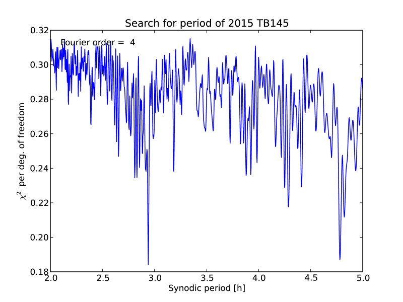
Figure 2: The resulting periodogram from our lightcurve analysis. There are two possible solutions: at (synodic) rotation period of 2.939 h (lowest $\chi^{2}$ solution), and 4.779 h (second best solution). Others have more than 10% higher $\chi^{2}$ values.

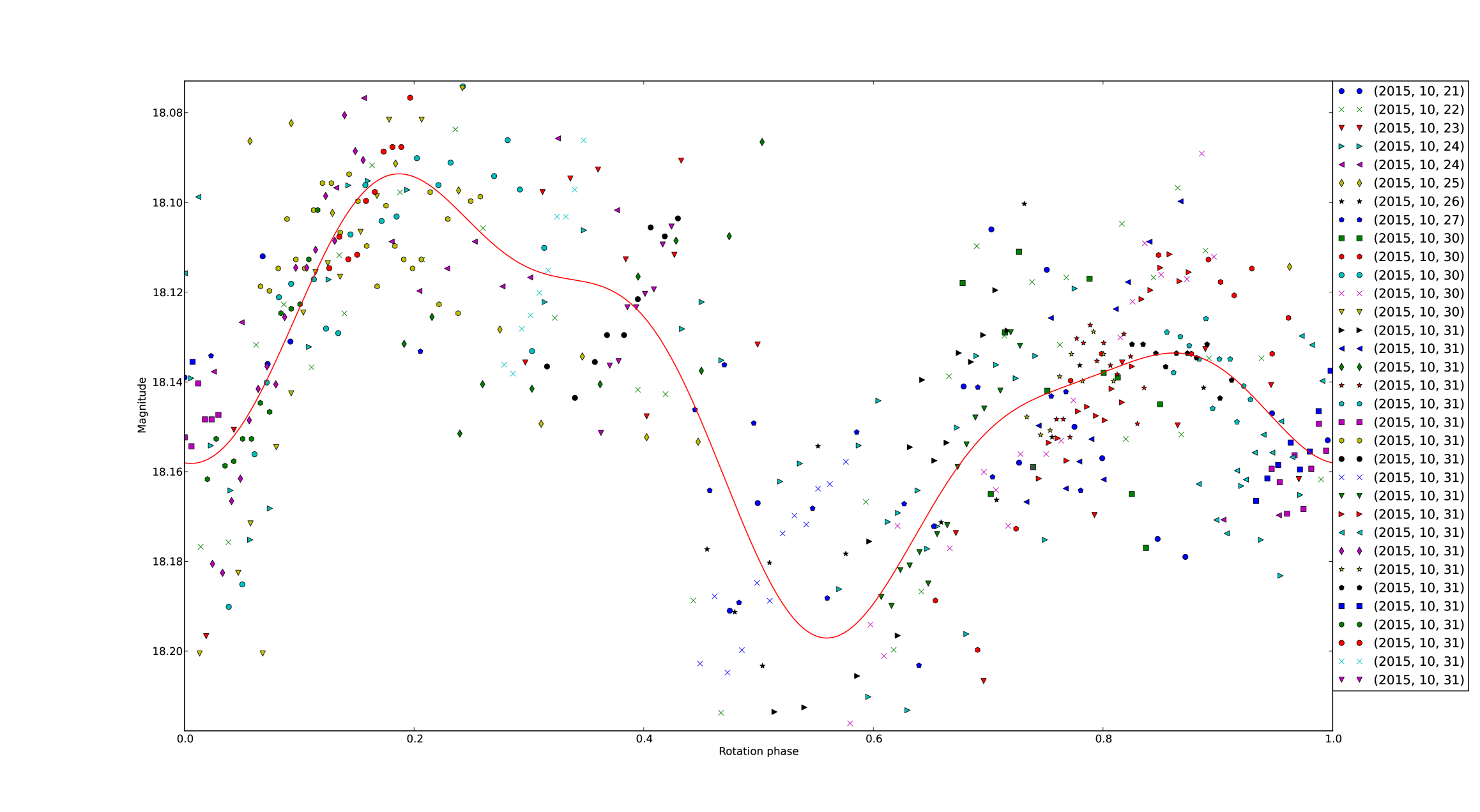
Figure 3: The best composite lightcurve from our Fourier analysis using relative magnitudes. Different telescopes and dates are indicated with different colours and/or symbols. The rotation period is 2.939 $\pm$ 0.005 h, with an amplitude of the 4^th-order Fourier fit of 0.12 $\pm$ 0.02 mag. The zero date used to fold the data is 2015 Oct. 21.3771 UTC (LT corrected).

On this combined dataset, we performed a Fourier analysis (see periodogram in Fig. 2) and found the best period at 2.939 $\pm$ 0.005 hours with the model lightcurve having an amplitude of 0.12 $\pm$ 0.02 mag (see Fig. 3), very close to the Warner et al. (warner16 (2016)) solution with 2.938 $\pm$ 0.002 h rotation period and 0.13 $\pm$ 0.02 mag amplitude. The second-lowest $\chi^{2}$ is found for a rotation period at 4.779 h (see Fig. 4). We consider the second solution less probable, as it implies a more complicated rarely-occurring 3-maxima lightcurve. Other solutions have $\chi^{2}$ values that are more than 10% higher than the one for the best solution and lead to a severe misfit of various fragments relative to one another. They can be excluded with high probability. To verify our results, we also used another algorithm based on pure $\chi^{2}$ fitting to search for the best composite lightcurves within a given range. The resulting composite is shown in Fig. 5, with a start date close to our first VLT-VISIR measurement. Both methods find the same (best) solution within the given error bars, given the poor quality of the data and large uncertainty range.

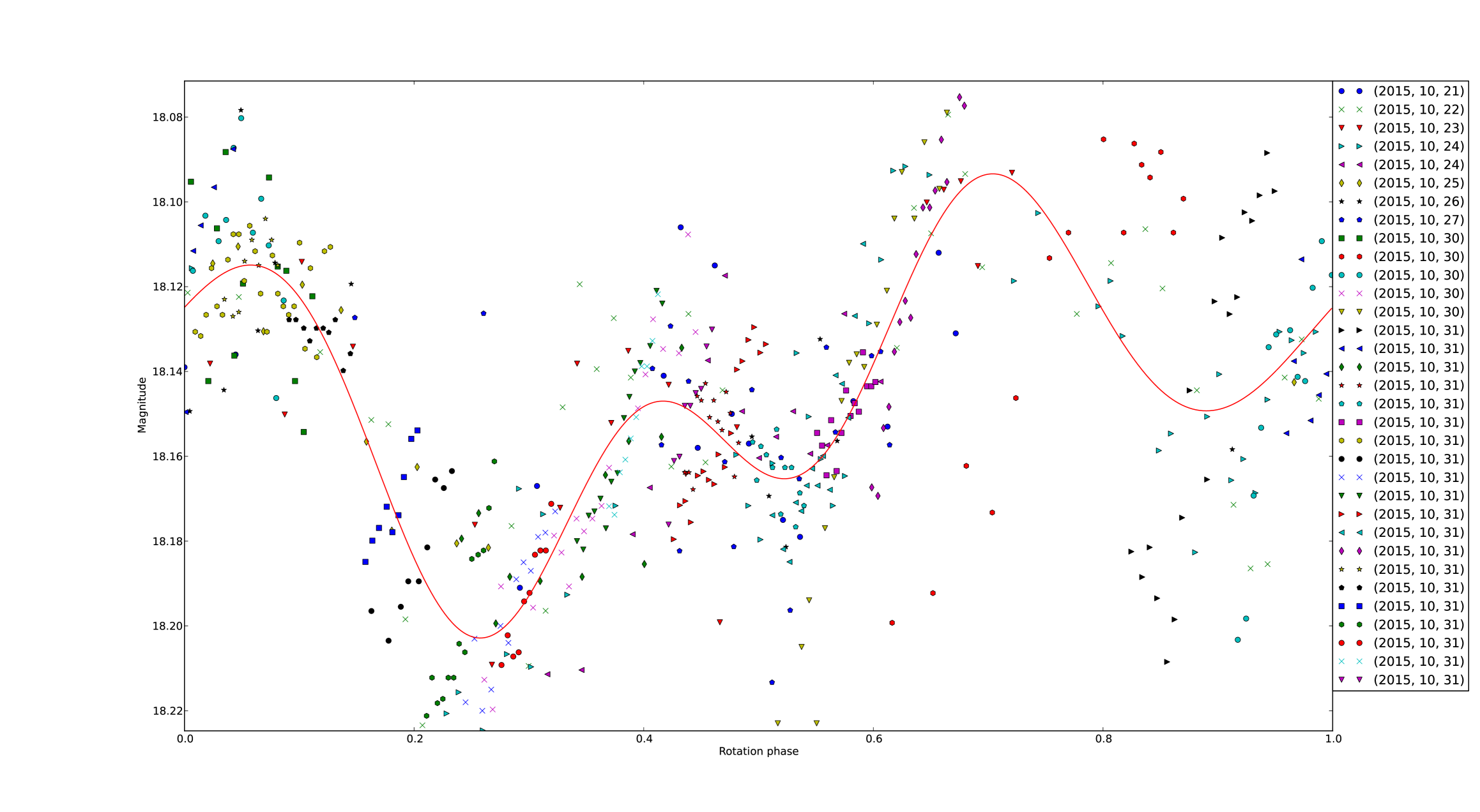
Figure 4: The second best composite lightcurve from our Fourier analysis. The rotation period is 4.779 $\pm$ 0.012 h, with an amplitude of the 4^th-order Fourier fit of 0.10 $\pm$ 0.02 mag. The zero date used to fold the data is 2015 Oct. 21.3771 UTC (LT corrected).

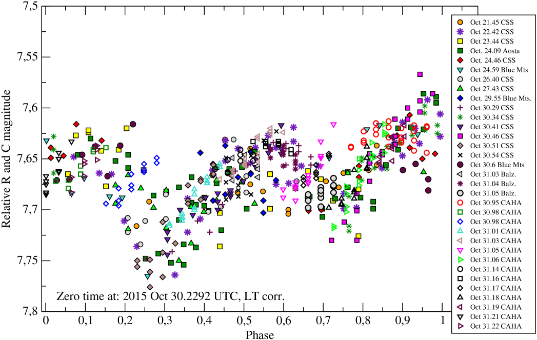
Figure 5: The composit lightcurve of 2015 TB₁₄₅ with a zero phase close to the start of the VLT-VISIR measurements (based on P = 2.941 $\pm$ 0.005 h, amplitude of 0.15 $\pm$ 0.03 mag, and zero phase at 2015, Oct 30.2292 UTC, LT corr.).

3.2 Absolute V-/R-magnitudes

Absolute magnitudes were obtained using the images from the OSN telescope as they were the only images obtained with a filter; the R-Johnson filter. For each star in the FOV with R magnitude in the USNOB1 catalog, we determined the magnitudes of the NEA and the star in 3-5 different images. The error was assumed to be the dispersion of the measured star magnitudes with respect to the catalogue star magnitudes. The obtained asteroid magnitude was then corrected by geocentric and heliocentric distances and by phase angle. Following the description in Bowell et al. (bowell89 (1989)), we calculated the H_R magnitude:

$$H_{R}(1,1,\alpha)=R_{mag}-5.0\cdot log(r\cdot\Delta)$$ (1)

$$H_{R}=H_{R}(1,1,\alpha)+2.5\cdot log((1-G)\cdot\phi\leavevmode\nobreak\ 1+G\cdot\phi\leavevmode\nobreak\ 2)$$ (2)

with $\alpha$ being the phase angle, R_mag the calibrated R-band magnitude of our target in the images, r the heliocentric distance, $\Delta$ the distance to the observer, H_R (1, 1, $\alpha$) is the R-band magnitude, at solar phase angle $\alpha$ reduced to unit heliocentric and geocentric distance, H_R is the absolute magnitude (at $\alpha$ = 0^∘), G the slope parameter (here we used the default value of 0.15), and $\phi$1 and $\phi$2 are two specified phase functions that are normalised to unity at $\alpha$ = 0^∘.

After the correction, we obtained the median of this H_R for the asteroid. In total, we determined seven different values (three for the night of Oct. 30, and four for the night of Oct. 29). The median of all seven values is H_R = 18.7 $\pm$ 0.2 mag.

As an alternative approach we used the Phase Curve Analyser tool (Oszkiewicz et al. oszkiewicz11 (2011); Oszkiewicz et al. oszkiewicz12 (2012)) and entered all available V- and R-band measurements from the MPC database. The phase curve analyser tool does not put any restraints on the slope parameters. Both absolute magnitude and slope parameters are fitted simultaneously, thus accounting for the different slopes of various taxonomic types. We found the following results:

• Based on the Bowell et al. (bowell89 (1989)) H-G conventions, the phase curve analyser tool produced H_R = 18.6 (with rms of the fit: 0.29 mag) and H_V = 19.3 mag (rms: 0.25 mag). This H_R solution is in excellent agreement with our own calibrated OSN measurements.

• Based on Muinonen et al. (muinonen10 (2010)) H-G₁₂ conventions, the phase curve analyser tool produced H_R = 19.18 mag and H_V = 19.75 mag. This is significantly different from the standard H-G assumptions, but, according to the authors, the H,G₁₂ phase function is applicable to asteroids with sparse or low-accuracy photometric data, which is the case for 2015 TB₁₄₅.

We use the H-G₁₂ solution in the following analysis and also discuss the impact of different values. It should be mentioned, however, that a reliable H magnitude cannot be derived from our data nor from the entries in the MPC astrometric database. The above values are, in effect, covering all possible slope values, which are not very well constrained. From the fitting of various phase functions (H-G, H-G₁₂, H-G₁-G₂) and taking the whole range of all possible solutions into account, we conservatively estimated a H-mag uncertainty of approximately 1 mag.

3.3 V-R colour

The above analysis leads to V-R colours of 0.7 mag (in the H-G system) and 0.6 mag (in the H-G₁₂ system). We also searched the MPC entries for measurements with V- and R-band observations taken by the same observatory (obs. code) during the same night (see Table 4).

Figure 6: V-R colour determination based on selected MPC entries.

Table 4: Number of MPC entries where V- and R-band measurements are listed for the same night by the same observer (observatory code). All measurements are from October 2015.

obs.	time span	meas. #
code	[days]	V	R	comments
C48	22.778 … 22.824	18	23	interchanged
Q62	24.540 … 24.612	6	8	sequential
Q62	26.503 … 26.767	26	3	sequential
C48	28.759 … 28.774	9	4	interchanged
C48	29.839 … 29.842	13	8	interchanged
585	31.065 … 31.080	49	60	interchanged

The entries from the Kyiv comet station (Ukraine) from Oct. 31, 2015, are the most consistent, and V- and R-band measurements are alternating. The summary of all data is shown in Fig. 6. Based on these data we calculated a V-R = 0.56 $\pm$ 0.05 mag which is confirmed by data from Oct. 22, 2015 for obscode C48 (0.55 mag), and also from Oct. 23 for obscode Q62 (0.57 mag). The other nights or datasets are more problematic with V- and R-band data appearing poorly balanced, covering different time periods or with large outliers. Our derived V-R finding agrees with values documented for other NEAs such as those by Pravec et al. (pravec95 (1995)) or Lin et al. (lin14 (2014)), for example.

4 Radiometric analysis

We used the derived properties from Section 3 together with the thermal measurements (Sect. 2) to calculate radiometric properties of the Halloween asteroid with standard thermophysical model techniques (see e.g. Müller et al. mueller13 (2013) or Müller et al. mueller16 (2016)). First, we consider a spherical shape model with a rotation period of 2.939 h and spin-axis orientations ranging from pole-on to equator-on during the VLT-VISIR observations. Size, albedo and thermal properties (thermal inertia $\Gamma$ and surface roughness) are free parameters in the analysis. Figure 7 shows the $\chi^{2}$ values for a very wide range of thermal inertias and as a function of spin-axis orientation. Here, we assumed a low surface roughness (r.m.s. of surface slopes of 0.1). The best fit to the VISIR data (accepting $\chi^{2}$ up to 20% above the minimum $\chi^{2}$) is found for thermal inertias in the range 250 to 700 Jm^-2s^-0.5K^-1 (retrograde rotation) and thermal inertias larger than 500 Jm^-2s^-0.5K^-1 (prograde rotation). The lowest $\chi^{2}$ values are connected to viewing geometries close to equator-on ($\pm$30^∘), with the spin axis roughly perpendicular to the line-of-sight. The best radiometric solutions for an equator-on viewing geometry and a surface roughness with r.m.s. of surface slopes of 0.1 are:

• prograde rotation (2.939 h): Thermal inertia $\Gamma$ = 900 Jm^-2s^-0.5K^-1; D_eff = 644 m, p_V = 5.5%;

• retrograde rotation (2.939 h): Thermal inertia $\Gamma$ = 400 Jm^-2s^-0.5K^-1; D_eff = 667 m, p_V = 5.1% (see also Fig. 8).

Based on the retrograde best solution, we produced plots with observation-to-model ratios as a function of wavelength and rotational phase (see Fig. 8). No obvious deviations or trends were visible. Our prograde best solution produces a similar match between measurements and model predictions.

Figure 7: The $\chi^{2}$ radiometric analysis of the VLT-VISIR data for a spherical shape solution, and for a range of different spin-axis orientations. The dashed horizontal line indicates a $\chi^{2}$ threshold 20% above the minium value. The solid lines show prograde cases (0^∘, +30^∘, and +45^∘ from a perfect equator-on geometry), the dashed-dotted lines are calculated for the same spin-axis orientations, but for retrograde cases. The dashed curve with $\chi^{2}$-values above 3 shows the pole-on geometry.

Figure 8: The VLT-VISIR observations divided by the corresponding TPM solution, assuming a spherical shape with a retrograde rotation (2.939 h rotation period), a size of 667 m, geometric albedo of 5.1%, thermal inertia of 400 Jm^-2s^-0.5K^-1 and low surface rougness (r.m.s. of surface slopes of 0.1). Top: ratios as a function of wavelength; bottom: as a function of rotational phase.

The same analysis for a high surface roughness (r.m.s. of surface slopes of 0.5) leads to thermal inertias shifted to higher values ($\Gamma$ $>$ 500 Jm^-2s^-0.5K^-1 for retrograde, and $\Gamma$ $>$ 1500 Jm^-2s^-0.5K^-1 for prograde rotation), with very similar size-albedo values. With our thermal dataset limited to a small wavelength range and a single epoch, it is not possible to break the degeneracy between thermal inertia and surface roughness: high-inertia combined with high surface roughness fits equally well as a low-inertia, low-roughness case.

The geometric V-band albedo p_V of 5-6% is tightly connected to our choice for the H magnitude. Assuming H_V = 19.3 mag (see H-G results in Section 3.2) would immediately lead to larger albedos of 8-9% whilst a larger H magnitude would produce smaller albedo values.

We also tested the influence of a longer rotation period of 2015 TB₁₄₅. A slower rotating body (4.779 h instead of 2.939 h) would shift the location of the $\chi^{2}$ minima in Fig. 7 to larger values: The best solution for a prograde rotation would be around a thermal inertia of 1250 Jm^-2s^-0.5K^-1 whilst the retrograde case would be best explained with an inertia of approximately 500 Jm^-2s^-0.5K^-1. Radiometric size and albedo solutions remain very similar.

The VISIR fluxes (mainly J8.9 data) show a sinusoidal change over time (most easily seen in Fig. 8 bottom, box symbols). If we interpret these variations as changes in the cross-section during the object’s rotation, we find a maximum effective size of approximately 680 m at thermal lightcurve maximum and approximately 650 m at lightcurve minimum. A rotating ellipsoidal shape (rotation axis $c$, equator-on viewing) with a/b=1.09 and b/c=1.0 would explain such a variation. A similar conclusion can be drawn from the observed visual lightcurve amplitude $\Delta$Mag = 0.12 $\pm$ 0.02 mag (see Fig. 3), which is pointing towards an axis ratio of a/b = 1.12, very similar to what we see in the varying thermal measurements. Also, the variations in visual brightness and thermal flux seem to be approximately in phase, with minima and maxima occurring at similar times. A firm statement is not possible, however, due to the error bars of the thermal measurements and the large scatter in visual brightness.

Table 5: Observational results. The ESO VLT-VISIR observations are related to the programme-ID 296.C-5007(A). The times and fluxes are related to the 2-nod averaged photometry. The flux errors include the errors of the aperture photometry (standard deviation of the eight individual fluxes from the 2-nod cycle images), a 3% error for the uncertainties in the models of the two calibration stars, and the error of the calibration factors.

Julian Date	$\lambda_{ref}$	FD	FDerr
mid-time	[$\mu$m]	[Jy]	[Jy]
2457325.74034	8.72	4.115	0.187
2457325.75106	8.72	4.116	0.184
2457325.76347	8.72	4.265	0.245
2457325.77852	8.72	4.548	0.226
2457325.79478	8.72	4.485	0.183
2457325.80909	8.72	4.509	0.194
2457325.82194	8.72	4.442	0.177
2457325.85373	8.72	4.828	0.285
2457325.86695	8.72	4.804	0.204
2457325.88110	8.72	4.826	0.208
2457325.74326	10.77	6.129	0.258
2457325.75526	10.77	6.344	0.268
2457325.76757	10.77	6.592	0.293
2457325.78568	10.77	6.664	0.280
2457325.80061	10.77	6.837	0.301
2457325.81363	10.77	7.026	0.306
2457325.82648	10.77	6.856	0.342
2457325.85789	10.77	7.385	0.321
2457325.87195	10.77	7.501	0.331
2457325.74587	11.88	6.575	0.317
2457325.75860	11.88	6.708	0.326
2457325.77186	11.88	7.023	0.303
2457325.78929	11.88	7.177	0.254
2457325.80398	11.88	7.191	0.306
2457325.81727	11.88	7.281	0.352
2457325.83013	11.88	7.199	0.283
2457325.86117	11.88	7.584	0.259
2457325.87613	11.88	7.643	0.293

5 Discussions

5.1 Rotation period

The Halloween asteroid is an interesting example for demonstrating the possibilities and limitations of radiometric techniques in cases of very limited observational data. The lightcurves cover only approximately ten days in total and the object had a very high apparent motion (up to several arcsec/sec) on the sky. It was therefore very difficult to extract reliable photometry from small field-of-view images and constantly changing reference stars. The construction of a full composite lightcurve from such short fragments is always very difficult and problematic. Here, the resulting large number of short and partly noisy lightcurve snippets led to two possible rotation periods (approximately 2.94 h and 4.78 h) in the periodogram (Fig. 2). A visual inspection of various possible periods was still needed, and the two remaining solutions were found to produce an acceptable fit of the various lightcurve fragments relative to each other. The thermal VISIR measurements also cover more than three hours, but, due to the low lightcurve amplitude, they do not put any additional constraints on the rotation period. In the end, the two derived rotation periods remain. Both have similar $\chi^{2}$ minima in the periodogram and the minima are within 10% of each other. All the periods are only synodic periods, however. Sidereal periods can only be determined with the help of full spin and shape model solutions, using data from multiple apparitions and/or a wide range of observing geometries. Our synodic periods are based on the single short apparition from October 2015, and they are only precise to within two or three decimals at best.

5.2 Spin-axis orientation

Single apparition visible lightcurves contain only very limited information about the orientation of the spin axis: a flat lightcurve can indicate either a pole-on viewing geometry (combined with arbitrary shape) or a spherical shape (with arbitrary orientation of the spin axis). Thermal data, however, can provide clues about the spin-axis orientation: a measurement of the shape of the spectral energy distribution contains information about the surface temperatures and these temperatures depend on the orientation of the spin axis and the thermal history of surface elements. Typically, a pole-on geometry produces much higher sub-solar temperatures (almost independent of the thermal properties of the surface) than a equator-on geometry where surface heat is constantly transported to the night side. Multi-band thermal measurements (single- or multiple-epoch data) can therefore be used to constrain the orientation of the object at the time of the observations. Here, the knowledge of the (approximate) rotation period is important for such investigations. In the case of our 3-band VISIR data we find that the observed spectral N-band slope is much better explained by temperatures connected to an equator-on viewing geometry. A pole-on temperature distribution would produce systematically higher J8.9 fluxes and lower PAH2_2, that is, a less-steep SED slope in the N-band wavelength range. These equator-on geometries correspond to a rotation axis pointing towards ($\lambda_{ecl}$, $\beta_{ecl}$) = (67^∘, +71^∘) for a prograde rotation and (67^∘, -71^∘) for a retrograde rotation ($\pm$ $\approx$30^∘).

A more accurate test would require thermal measurements covering a wider wavelength range. The VISIR instrument is equipped with an M-band filter (bandpass 4.54 - 5.13 $\mu$m), but no M-band measurements were included in our programme. In this context, we also searched for possible NEOWise (Mainzer et al. mainzer14 (2014)) detections at shorter wavelengths (3.4 and 4.6 $\mu$m), but our target was either too faint (Jun. and Nov. 2014, Aug. 2015, Jun. 2016) or too bright (Oct. 2015). In Oct. 2015, the Halloween asteroid was very close to Earth and it crossed the solar elongation zone visible by NEOWise (approximately 87^∘ - 93^∘) with an apparent motion of more than 10^′′/s. At the same time, the object was extremely bright with an estimated W2 (4.6 $\mu$m) flux of more than 10 Jy, well above the NEOWise saturation limits. We are not aware of any other auxiliary thermal measurements of 2015 TB₁₄₅.

5.3 Thermal inertia

If we look at an object pole-on, the temperature distribution does not depend significantly on the thermal inertia of the surface, but it does have a significant effect on viewing geometries close to equator-on: a large thermal inertia transports more engery to the night side than a low thermal inertia, and the sense of rotation determines if we see a warm or cold terminator. In our case, we observed the object at approximately 34^∘ phase angle. The prograde rotation requires a relatively large thermal inertia close to 1000 Jm^-2s^-0.5K^-1 to explain our measurements, while a retrograde rotation would lead to $\Gamma$-values close to 400 Jm^-2s^-0.5K^-1. It is not possible to distinguish these two cases from our limited observations. These two minima also depend on the object’s rotation period: taking the second-best period (approximately 5 h) would shift both $\Gamma$-minima to larger values at approximately 500 Jm^-2s^-0.5K^-1 (retrograde) and 1250 Jm^-2s^-0.5K^-1 (prograde). A similar effect can be seen when changing the surface-roughness settings in the TPM: rougher surfaces lead to larger thermal inertias in the radiometric analysis. This degeneracy cannot be completely broken by our limited observations. One would need more thermal data from different phase angles (before and after opposition) combined with data from a wider wavelength range to be able to distinguish between roughness and thermal inertia effects. Here in our case, the fit to the measurements is better when assuming low-roughness surfaces (r.m.s. of surface slopes below 0.5) with $\chi^{2}$ minima close to 1.0. Very high-roughness cases, similar to the pole-on geometries, lead to poor fits to our measurements and the corresponding $\chi^{2}$ minima are far from 1.0. Overall, NEAs tend to have thermal inertias well below 1000 Jm^-2s^-0.5K^-1 (Delbo et al. delbo15 (2015)). If we accept this as a general (natural?) limit, then we have to conclude that 2015 TB₁₄₅ is very likely to have a retrograde rotation and that the most-likely thermal inertia is approximately 400-500 Jm^-2s^-0.5K^-1. Based on our limited coverage of the object’s SED, and unkowns in rotation period, surface roughness, and possibly also the presence of shallow spectral features, the derived inertias have considerable uncertainties. For our retrograde solution we find that the thermal measurements are compatible with $\Gamma$-values in the range 250 to 700 Jm^-2s^-0.5K^-1.

5.4 Size

Radiometric techniques are known to produce highly-reliable size estimates (e.g. Müller et al. mueller14 (2014), and references therein). But in cases with limited observational data from only one apparition, the situation is less favorable. Unknowns in the object’s rotational properties lead directly to large error bars for the derived thermal inertias. For our retrograde, equator-on situation we find thermal inertias from 250 to 700 Jm^-2s^-0.5K^-1 for a best-fit to the thermal slope. The translation into radiometric sizes produces values between 630 m (low $\Gamma$) and 695 m (high $\Gamma$). A rougher surface would also require higher thermal inertias, but the resulting sizes would be very similar. Also, a longer rotation period pushes the acceptable inertias to slightly larger values, but roughly equal sizes. First indications from radar measurements gave a size estimate of approximately 600 m. Our analysis shows that even extreme settings (low roughness, fast rotation and perfect equator-on geometry) would require thermal inertias below 150 Jm^-2s^-0.5K^-1 to produce a radiometric size of 600 m. The corresponding reduced $\chi^{2}$ value in Fig. 7 is above 1.5 and the fit (especially to the J8.9 data) is very poor. However, we cannot completely rule out the 600-m size (in combination with a thermal inertia of approximately 100-200 Jm^-2s^-0.5K^-1). One explanation could be that fine-grained regolith material affects the surface emissivity in a strongly wavelength-dependent way (while we assume a flat emissivity of 0.9), with approximately 10% higher emissivities in the SIV_2 band compared to the J8.9 band. Studying the emissivity variations found for three Trojans (Emery et al. emery06 (2006)), however, we believe that such strong variations in the 9-12 $\mu$m range are not possible. The poor $\chi^{2}$ fit of a 600-m body (with or without spectral emission features in the N-band) make such a size-solution very unlikely. Taking all these aspects into account, we estimate a minimum size of approximately 625 m, and a maximum of just below 700 m for the NEA 2015 TB₁₄₅. Our best-fit value is 667 m ($\Gamma$ = 400 Jm^-2s^-0.5K^-1, retrograde rotation) or 644 m ($\Gamma$ = 900 Jm^-2s^-0.5K^-1, prograde rotation).

An independent NEATM approach (Harris harris98 (1998)) in analysing the VISIR measurements confirms our large size for 2015 TB₁₄₅ which exceeds the radar estimates. Figure 9 shows the results in terms of size as a function of the beaming parameter $\eta$ (top) and the fit to our averaged 3-band fluxes connected to the observing geometry at half way through the VISIR measurements (see Tables 3 and 5). For these calculations we assumed a spherical shape and a wide range for $\eta$. We determined the radiometric NEATM size for each $\eta$ together with the corresponding reduced $\chi^{2}$ value. The best fit is found for a size of D = 690 m, $\eta$ = 1.95 and a geometric V-band albedo p_V = 0.05 (assuming H_V = 19.75 mag).

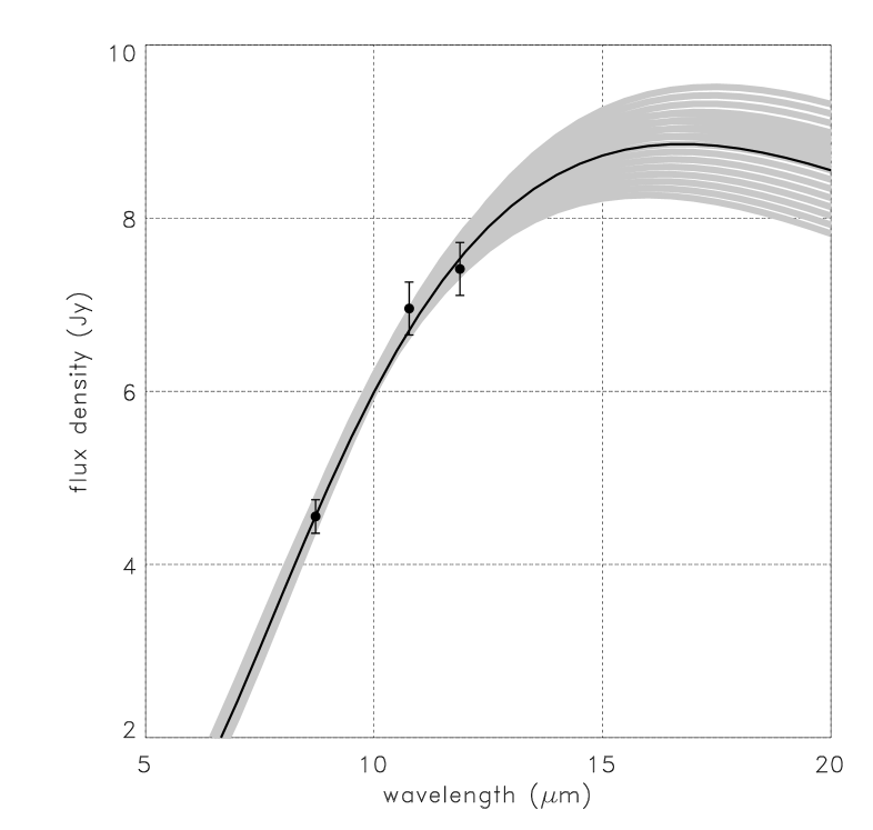
Figure 9: NEATM analysis of averaged 3-band VISIR data. Contours in the diameter-$\eta$ plot (top) correspond to reduced $\chi^{2}$ values of 1.0, 1.3, 1.6, and 1.9. The best-fit solution (bottom) is shown as a solid black line. Grey curves have $\chi^{2}_{red}$ below 1.9.

The optimum $\eta$ is relatively high, but justified considering the fast rotation (2.9 h) of a kilometer-sized object. There is a strong correlation between the possible diameters and $\eta$ values and a simple error estimate is not easy, but following the previous TPM analysis, the object’s size is found to be significantly larger than 600 m.

5.5 Albedo

Calculation of the geometric albedo requires a robust estimate of the object’s absolute magnitude. Here again, the H-magnitude calculations suffer from low-quality single-apparition measurements. Our case with observations from an extremely restricted phase angle range is probably not typical, but often the H-mag calculations suffer from unknowns in the phase relation. Our own calibrated R-band measurements are all taken close to 34^∘ phase angle and the MPC R-/V-band database entries were optimised for astrometric calculations and have no error bars. Simply plotting the reduced magnitudes from MPC shows scatter on a 1-2 magnitude scale within a given night, bearing in mind that the object’s lightcurve amplitude is only approximately 0.1 mag. We applied different techniques to derive an absolute magnitude: the two methods, standard H-G and H-G₁₂ , produce H_V solutions of 19.3 mag and 19.75 mag, respectively. The true uncertainty could even be in the order of 1-2 mag, depending on the different phase functions and fitting routines (non-linear vs. linear). Such large uncertainties are probably common among the single-apparition NEAs. In the absence of thermal measurements, these H-mag estimates are commonly used to derive sizes for low- and high-albedo assumptions. Here, a 19 mag value for a low-albedo (p_V = 0.03) object leads to a size estimate above 1.2 km, while 20 mag combined with p_V = 0.5 would result in a size estimate of 188 m, smaller in size by a factor of over 6. Adding thermal data changes the situation dramatically and produces reliable size-albedo solutions. However, using a H-mag of 19.0 pushes the geometric albedo to approximately 10%, while an absolute magnitude of 20.0 would give a 4% albedo. This uncertainty in albedo can only be reduced with more reliable photometric data points spread over a wider phase angle range.

5.6 Shape

Both the visual lightcurves and the thermal measurements show brightness/flux variations over timescales of a few hours. After correcting for the rapidly changing observing geometries, we find lightcurve amplitudes close to 10%. This is compatible with a rotating ellipsoid with an axis ratio a/b = 1.1 seen equator-on. More elongated bodies are also possible, but then in combination with a different obliquity for the spin axis. An extreme axis ratio of a very elongated object can be excluded with high probability, mainly because of the observed thermal emission spectrum which can be best explained by equator-on viewing geometries. On the other hand, a regular ellipsoidal shape can also be excluded by the strong deviations of the lightcurve from a sinosoidal shape (see Figs. 3, 4, and 5).

6 Conclusions

NEAs with very close encounters with Earth always receive great attention from the public. It is usually also relatively easy to obtain high-S/N photometry during the encounter phase, even with small telescopes and for very small objects. However, a reliable and high-quality physical and thermal characterisation of the objects with single-apparition data is often challenging. The Halloween asteroid had an encounter with Earth at 1.3 lunar distances on October 31, 2015, and nicely illustrates the possibilities and limitations of current analysis techniques.

The calculation of a reliable H-magnitude is difficult and depends strongly on a good photometric coverage over wide phase angle ranges. For 2015 TB₁₄₅ there are no measurements available at phase angles below 33^∘ and we obtained H_V magnitudes between 19 and 20 mag, depending on the applied phase relation. Using the H-G₁₂ conventions for sparse and low-accuracy photometric data (Muinonen et al. muinonen10 (2010)), we find H_R = 19.2 mag and H_V = 19.8 mag, with large uncertainties which could easily be up to one magnitude (conservative estimate based on fitting various phase functions (H-G, H-G₁₂, H-G₁-G₂) and taking the whole range of all possible solutions and uncertainties into account). The determination of the object’s V-R colour is more reliable and based on different calculations and different data sets, we find a V-R colour of 0.56 $\pm$ 0.05 mag.

We combined lightcurve observations from different observers with our own measurements. The Fourier analysis periodogram shows several possible rotation periods, with two periods producing best $\chi^{2}$ minima and an acceptable fit of various lightcurve fragments relative to each other: 2.939 $\pm$ 0.005 hours (amplitude 0.12 $\pm$ 0.02 mag) and 4.779 $\pm$ 0.012 h (amplitude 0.10 $\pm$ 0.02 mag). A similar lightcurve amplitude is also seen in the thermal measurements (after correcting for the rapidly changing Earth-NEA distance), but measurement errors are too large to constrain the rotation period.

The detemination of the object’s spin axis orientation is not possible from such sets of lightcurves. 2015 TB₁₄₅ was observable only for approximately two weeks in October 2015 and neither the phase angle bisector nor the phase angle changed significantly and no noticeable change in rotation period or amplitude was seen (Warner et al. warner16 (2016)) (also confirmed by our additional lightcurve data).

For our TPM radiometric analysis we find 2015 TB₁₄₅ was very likely close to an equator-on observing geometry ($\pm$ $\approx$30^∘) during the time of the VLT-VISIR measurements. A pole-on geometry can be excluded from the observed 8-12 $\mu$m emission slope from the multiple 3-filter N-band measurements. In the process of radiometric size and albedo determination from the combined thermal data set we find the object’s thermal inertia to be between 250 to 700 Jm^-2s^-0.5K^-1 in case of a retrograde rotation, and above $\approx$500 Jm^-2s^-0.5K^-1 for a prograde rotation. These ranges are found for an equator-on observing geometry of a spherical body with 2.939 h rotation period and a low surface roughness (r.m.s. of surface slopes of 0.1). Moving away from an equator-on geometry, or using longer rotation periods or higher surface roughness would shift these thermal inertia ranges to larger values. The maximum (model) surface temperatures during our VISIR measurements are close to 350 K, (equator-on geometry) or even above in case of a spin axis closer to a pole-on geometry. From our radiometric TPM analysis we estimate a minimum size of approximately 625 m, and a maximum of just below 700 m for the NEA 2015 TB₁₄₅ (the corresponding NEATM diameter range is between 620 and 760 m, for beaming parameters $\eta$ of 1.6 and 2.2, respectively, and best-fit values at 690 m for $\eta$ = 1.95). The best match to all thermal measurements is found for: (i) Thermal inertia $\Gamma$ = 900 Jm^-2s^-0.5K^-1; D_eff = 644 m, p_V = 5.5% (prograde rotation with 2.939 h); (ii) thermal inertia $\Gamma$ = 400 Jm^-2s^-0.5K^-1; D_eff = 667 m, p_V = 5.1% (retrograde rotation with 2.939 h).

The reconstruction of the object’s shape is not possible, but an equator-on viewing geometry combined with the visual and thermal lightcurve amplitude would point to an ellipsoidal shape with an axis ratio a/b of approximately 1.1 (assuming a rotation around axis $c$).

Following the discussions and formulas in Gundlach & Blum (gundlach13 (2013)) we can also estimate possible grain sizes on the surface of the NEA 2015 TB₁₄₅. For the calculations we used the CM2 meteoritic sample properties (matching our low albedo of approximately 5%) from Opeil et al. (opeil10 (2010)), with a density $\rho$ = 1700 kg m^-3, and a specific heat capacity of the regolith particles $c$ = 500 J kg^-1 K^-1. A thermal inertia of 400 Jm^-2s^-0.5K^-1 leads to heat conductivities $\lambda$ in the range 0.3-1.9 W K^-1 m^-1, or 2-12 W K^-1 m^-1 for a thermal inertia of 1000 Jm^-2s^-0.5K^-1. The estimated grain sizes would then be in the order of 10-20 mm ($\Gamma$ = 400 Jm^-2s^-0.5K^-1) or 50-100 mm ($\Gamma$ = 1000 Jm^-2s^-0.5K^-1), considering a wide range of regolith volume-filling factors from 0.1 (extremely fluffy) to 0.6 (densest packing).

Based on our analysis and careful inspection of the available data, we make several recommendations for future observations of similar-type objects:

1. Size estimates for single-apparition NEAs from H-magnitudes alone are highly uncertain. The estimates depend on assumptions for the albedo, but also suffer from possible huge uncertainties in H-magnitudes which can easily reach 1-2 mag. Here, without thermal data, one would estimate a size below 200 m (H = 20.0, p_V = 0.5) or above 1.2 km (H = 19.0, p_V = 0.03). Having a more accurate H-magnitude would shrink the possible sizes to values between approximately 250 and 950 m.

2. For the determination of reliable H-magnitudes it is essential to have calibrated R- or V-band photometric data points spread over a wide range of phase angles, preferably also including small phase angles below 7.5^∘.

3. For a good-quality physical characterisation (radiometric analysis and also the interpretation of radar echos) it is important to find the object’s rotational properties. This requires high-quality lightcurves: (i) in cases of very short rotation periods it is important to avoid rotational smearing, with exposures well below $\approx$0.2 of the rotation period (Pravec et al. pravec00 (2000)); (ii) for rotation periods of several hours or longer there is the challenge of covering substantial parts of the lightcurve of very fast-moving objects with one set of reference stars; rapidly changing image FOVs cause severe problems in reconstructing the composite lightcurve. Thus, observing instruments with large FOVs of the order of one or a few degrees are recommended.

4. For thermal measurements of NEAs it is very helpful to have (i) the widest possible wavelength coverage, possibly also including M- or Q-bands, to constrain the thermal inertia from the reconstructed thermal emission spectrum; (ii) well-calibrated measurements (calibration stars close in flux, airmass, time and location on the sky) to derive reliable size estimates; (iii) observations before and after opposition at different phase angles to determine the sense of rotation, to put strong constraints on thermal inertia and to break the degeneracy between thermal inertia and surface roughness effects.

The next encounter of 2015 TB₁₄₅ with Earth is in November 2018 at a distance of approximately 0.27 AU and with an apparent magnitude of approximately 19.5 mag. During that apparition it would easily be possible to get reliable R-band lightcurves for 2015 TB₁₄₅. The object will reach approximately 5, 60 and 90 mJy at 5, 10 and 20 $\mu$m, respectively, detectable with useful S/N ratios with ground-based MIR instruments such as VLT/VISIR. In the future, with telescope sizes well above 10 m, one can expect to study Apollo asteroids comparable to 2015 TB₁₄₅ out to distances of up to 0.5 AU.

- (1) Bowell, E. 1989, Asteroids II; Proceedings of the Conference, Tucson, AZ, Mar. 8-11, 1988 (A90-27001 10-91), University of Arizona Press, 1989, p. 524-556
- (2) Cohen, M., Walker, R. G., Carter, B. et al. 1999, AJ, 117, 1864-1889
- (3) Delbo, M., Mueller, M., Emery, J. P. et al. 2015, in Asteroids IV, P. Michel, F. E. DeMeo, W. F. Bottke (eds.), University of Arizona Press, Tucson, 107-128
- (4) Emery, J. P., Cruikshank, D. P., Van Cleve, J. 2006, Icarus, 182, 496
- (5) Gundlach, B. & Blum, J. 2013, Icarus 223, 479-492
- (6) Harris, A. W. 1998, Icarus 131, 291
- (7) Käufl, H. U., Kerber, F., Asmus, D. et al. 2015 The Messenger, 159, 15-18
- (8) Lagage, P. O., Pel, J. W., Authier, M. et al. 2004, The Messenger 117, 12-16
- (9) Licandro, J., Müller, T., Alvarez, C. et al. 2016, A&A 585, 10L
- (10) Lin, C.-H. Ip, W.-H., Lin, Z.-Y. et al. 2014 Research in Astronomy and Astrophysics 14, 311
- (11) Mainzer, A., Bauer, J., Cutri, R. M. et al. 2014, ApJ, 792, 30M
- (12) Müller, T. G., Sekiguchi, T., Kaasalainen, M. et al. 2005, A&A, 443, 347-355
- (13) Müller, T. G., Miyata, T., Kiss, C. et al. 2013, A&A, 558, 97
- (14) Müller, T. G., Hasegawa, S. & Usui, F. 2014, PASJ, 66, 52M
- (15) Müller, T. G., Ďurech, J., Ishiguro, M. et al. 2016 A&A, submitted
- (16) Muinonen, K., Belskaya, I. N., Cellino, A. et al. 2010, Icarus, 209, 542
- (17) Opeil, C.P., Consolmagno, G.J., Britt, D.T. 2010, Icarus 208, 449-454
- (18) Oszkiewicz, D. A., Muinonen, K., Bowell, E. et al. 2011, Journal of Quantitative Spectroscopy and Radiative Transfer 112, 1919-1929
- (19) Oszkiewicz, D. A., Bowell, E., Wasserman, L. H. et al. 2012, Icarus 219, 283-296
- (20) Pravec, P., Wolf, M., Varady, M., and Bárta, P. 1995, EM&P, 71, 177
- (21) Pravec, P., Hergenrother, C., Whiteley, R. et al. (2000), Icarus 147, 477-486
- (22) Schütz, O. & Sterzik, M. 2005, in High Resolution Infrared Spectroscopy in Astronomy, Proceedings of an ESO Workshop held at Garching, Germany, 18-21 November 2003. Käufl, Siebenmorgen, Moorwood (Eds.), 104
- (23) Vokrouhlický, D., Farnocchia, D., Čapek, D. et al. 2015, Icarus, 252, 277
- (24) Warner, B. D., Carbognani, A., Franco, L., Oey, J. 2016, The Minor Planet Bulletin, Vol. 43, No. 2, pp. 141-142