Modulation of unpolarized light in planar aligned subwavelength-pitch deformed-helix ferroelectric liquid crystals

Abstract

We study the electro-optic properties of subwavelength-pitch deformed-helix ferroelectric liquid crystals (DHFLC) illuminated with unpolarized light. In the experimental setup based on the Mach-Zehnder interferometer, it was observed that the reference and the sample beams being both unpolarized produce the interference pattern which is insensitive to rotation of in-plane optical axes of the DHFLC cell. We find that the field induced shift of the interference fringes can be described in terms of the electrically dependent Pancharatnam relative phase determined by the averaged phase shift, whereas the visibility of the fringes is solely dictated by the phase retardation.

I Introduction

Liquid crystal (LC) spatial light modulators (SLMs) are known to be the key elements widely employed to modulate amplitude, phase, or polarization of light waves in space and time Efron (1995). Ferroelectric liquid crystals (FLCs) represent most promising chiral liquid crystal material which is characterized by very fast response time (a detailed description of FLCs can be found, e.g., in Oswald and Pieranski (2006)). However, most of the FLC modes are not suitable for phase-only modulation devices because their optical axis sweeps in the plane of the cell substrate producing undesirable changes in the polarization state of the incident light.

In order to get around the optical axis switching problem the system consisting of a FLC half-wave plate sandwiched between two quarter-wave plates was suggested in Love and Bhandari (1994). But, in this system, the $2\pi$ phase modulation requires the smectic tilt angle to be equal to 45^∘. This value is a real challenge for the material science and, in addition, the response time dramatically increases when the tilt angle grows up to 45^∘ Barnik et al. (1987); Pozhidaev et al. (1988).

An alternative approach proposed in Pozhidaev et al. (2013, 2014) is based on the orientational Kerr effect in a vertically aligned deformed helix ferroelectric LC (DHFLC) with subwavelength helix pitch. This effect is characterized by fast and, under certain conditions Blinov et al. (2005); Pozhidaev et al. (2012), hysteresis-free electro-optics that preserves ellipticity of the incident light.

An important point is that all the above mentioned studies deal with the case of linearly polarized illumination where the incident beam is fully polarized. In this paper, we will go beyond this limitation and examine the electro-optic behavior of the planar aligned DHFLC cells illuminated with unpolarized light as the way to obtain the response insensitive to the effect of electric-field-induced rotation of in-plane optical axes which was found to be responsible for the presence of amplitude modulation Kotova et al. (2015). The paper is organized as follows.

In Sec. II, after introducing the geometry of the DHFLC cell and discussing the orientational Kerr effect, we describe the samples and our experimental setup which is based on the Mach-Zehnder interferometer. The experimental results are interpreted theoretically in Sec. III. Finally, in Sec. IV we draw the results together and make some concluding remarks. Details on the effective dielectric tensor of DHFLC cells are given in the Appendix.

II Experiment

We consider a DHFLC layer of thickness $D$ with the $z$ axis normal to the bounding surfaces: $z=0$ and $z=D$ (see Fig. 1). The geometry of a uniform lying DHFLC helix with subwavelength pitch where the helix (twisting) axis $\hat{\mathbf{h}}$ is directed along the $x$ axis will be our primary concern. In this geometry depicted in Fig. 1 the equilibrium orientational structure can be described as a helical twisting pattern where FLC molecules align on average along a local unit director

$$\hat{\mathbf{d}}=\cos\theta\,\hat{\mathbf{h}}+\sin\theta\,\hat{\mathbf{c}},$$ (1)

where $\theta$ is the smectic tilt angle; $\hat{\mathbf{h}}=\hat{\mathbf{x}}$ is the twisting axis normal to the smectic layers and $\hat{\mathbf{c}}\perp\hat{\mathbf{h}}$ is the $c$-director. The FLC director (1) lies on the smectic cone depicted in Fig. 1(left) and rotates in a helical fashion about a uniform twisting axis $\hat{\mathbf{h}}$ forming the FLC helix. This rotation is described by the azimuthal angle around the cone $\phi$ that specifies orientation of the $c$-director in the plane perpendicular to $\hat{\mathbf{h}}$.

Figure 1(right) illustrates the uniform lying FLC helix in the slab geometry with the smectic layers normal to the substrates and

$$\hat{\mathbf{h}}=\hat{\mathbf{x}},\quad\hat{\mathbf{c}}=\cos\phi\,\hat{\mathbf{y}}+\sin\phi\,\hat{\mathbf{z}},\quad\mathbf{E}=E\,\hat{\mathbf{z}},$$ (2)

where $\mathbf{E}$ is the applied electric field which is linearly coupled to the spontaneous ferroelectric polarization

$$\mathbf{P}_{s}=P_{s}\hat{\mathbf{p}},\quad\hat{\mathbf{p}}=\hat{\mathbf{h}}\times\hat{\mathbf{c}}=\cos\phi\,\hat{\mathbf{z}}-\sin\phi\,\hat{\mathbf{y}},$$ (3)

where $\hat{\mathbf{p}}$ is the polarization unit vector.

For a biaxial FLC, the components of the dielectric tensor, $\boldsymbol{\varepsilon}$, are given by

$$\epsilon_{ij}=\epsilon_{\perp}\delta_{ij}+(\epsilon_{1}-\epsilon_{\perp})\,d_{i}d_{j}+(\epsilon_{2}-\epsilon_{\perp})\,p_{i}p_{j}$$

$$=\epsilon_{\perp}[\delta_{ij}+(r_{1}-1)d_{i}d_{j}+(r_{2}-1)p_{i}p_{j}],$$ (4)

where $i,j\in\{x,y,z\}$, $\delta_{ij}$ is the Kronecker delta; $d_{i}$ ($p_{i}$) is the $i$th component of the FLC director [unit polarization vector] given by Eq. (1) [Eq. (3)]; $r_{1}=\epsilon_{1}/\epsilon_{\perp}$ ($r_{2}=\epsilon_{2}/\epsilon_{\perp}$) is the anisotropy (biaxiality) ratio. In the case of uniaxial anisotropy with $r_{2}=1$, we have the two principal values of the dielectric tensor, $\epsilon_{2}=\epsilon_{\perp}$ and $\epsilon_{1}=\epsilon_{\parallel}$, giving the ordinary (extraordinary) refractive index $n_{\perp}=\sqrt{\mu\epsilon_{\perp}}$ ($n_{\parallel}=\sqrt{\mu\epsilon_{\parallel}}$), where the magnetic tensor of FLC is assumed to be isotropic with the magnetic permittivity $\mu$.

According to Refs. Kiselev et al. (2011); Kiselev and Chigrinov (2014); Kotova et al. (2015), optical properties of such cells can be described by the effective dielectric tensor of a homogenized DHFLC helical structure (the results used in this paper are summarized in the Appendix). As is shown in Fig. 2, the zero-field ($\mathbf{E}=0$) dielectric tensor is uniaxially anisotropic with the optical axis directed along the twisting axis $\hat{\mathbf{h}}=\hat{\mathbf{x}}$. The zero-field effective refractive indices of extraordinary (ordinary) waves, $n_{h}$ ($n_{p}$), generally depend on the smectic tilt angle $\theta$ and the optical (high frequency) dielectric constants characterizing the FLC material that enter the tensor given in Eq. (4) (the expressions for $\epsilon_{h}=n_{h}^{2}$ and $\epsilon_{p}=n_{p}^{2}$ are given by Eq. (37) in the Appendix).

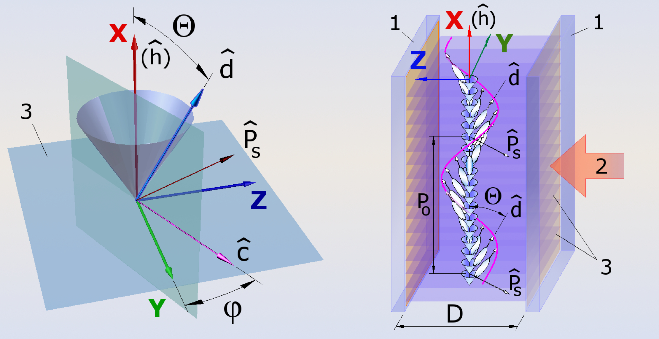
Figure 1: Geometry of smectic cone (left) and DHFLC cell (right). 1 – cell substrates; 2 – incident light beam; 3 – smectic layers.

Referring to Fig. 2, the electric-field-induced anisotropy is generally biaxial so that the dielectric tensor is characterized by the three generally different principal values (eigenvalues): $\epsilon_{\pm}=n_{\pm}^{2}$ and $\epsilon_{z}=n_{z}^{2}$ (see Eqs. (40) and (41) in the Appendix). The in-plane principal optical axes (eigenvectors)

$$\hat{\mathbf{d}}_{+}=\cos\psi_{d}\,\hat{\mathbf{x}}+\sin\psi_{d}\,\hat{\mathbf{y}},\quad\hat{\mathbf{d}}_{-}=\hat{\mathbf{z}}\times\hat{\mathbf{d}}_{+}$$ (5)

are rotated about the vector of electric field, $\mathbf{E}\parallel\hat{\mathbf{z}}$, by the azimuthal angle $\psi_{\mathrm{d}}$ (see Eq. (46) in the Appendix). In the low electric field region, the electric field dependence of the angle $\psi_{\mathrm{d}}$ is approximately linear: $\psi_{\mathrm{d}}\propto E$, whereas the electrically induced part of the principal refractive indices, $n_{\pm}$ and $n_{z}$, is typically dominated by the Kerr-like nonlinear terms proportional to $E^{2}$ (see, e.g., equations (10)–(18) in Ref. Kotova et al. (2015)). This effect  —  the so-called orientational Kerr effect —  is caused by the electrically induced distortions of the helical structure. It is governed by the effective dielectric tensor of a nanostructured chiral smectic liquid crystal defined through averaging over the FLC orientational structure Pozhidaev et al. (2013, 2014); Kiselev et al. (2011); Kiselev and Chigrinov (2014).

Figure 2: Ellipsoids of effective refractive indices of a short-pitch DHFLC cell. Left: at $\mathbf{E}=0$, the field-free effective ellipsoid is uniaxially anisotropic with the optical axis parallel to the helix axis (the $x$ axis). The refractive indices $n_{h}$ and $n_{p}$ correspond to the optical axes along and perpendicular to the helix axis, respectively. Right: applying an electric field across the cell, makes the optical anisotropy biaxial with the two in-plane optical axes rotated by the angle $\psi_{d}\propto E$ about the electric field vector $\mathbf{E}$.

In our experiments we have used the FLC mixture FLC-624 (from P.N. Lebedev Physical Institute of Russian Academy of Sciences) as the material for the DHFLC layer. The FLC-624 is a mixture of the FLC-618 (the chemical structure can be found in Pozhidaev et al. (2014)) and the well-known nematic liquid crystal 5CB. The weight concentrations in the mixture are 98% of FLC-618 and 2% of 5CB. The phase transition sequence of the FLC-624 during heating from the solid crystalline phase is $\mathrm{Cr}\xrightarrow{+20^{\circ}\mathrm{C}}\mathrm{Sm}C^{\star}\xrightarrow{+60^{\circ}\mathrm{C}}\mathrm{Sm}A^{\star}\xrightarrow{+116^{\circ}\mathrm{C}}\mathrm{Iso},$ whereas at cooling down from isotropic phase crystallization occurs around +6^∘C. At room temperature ($T=23^{\circ}$C), the spontaneous polarization $P_{s}$ and the FLC helix pitch $p_{0}$ are $185$ nC/cm² and $210$ nm, respectively.

The FLC-624 layer is sandwiched between two glass substrates covered by indium tin oxide (ITO) and aligning films with the thickness $20$ nm and the gap is fixed by spacers at $D\approx 53$ $\mu$m. The FLC alignment technique that provides high-quality chevron-free planar alignment with smectic layers perpendicular to the substrates is detailed in Ref. Kotova et al. (2015).

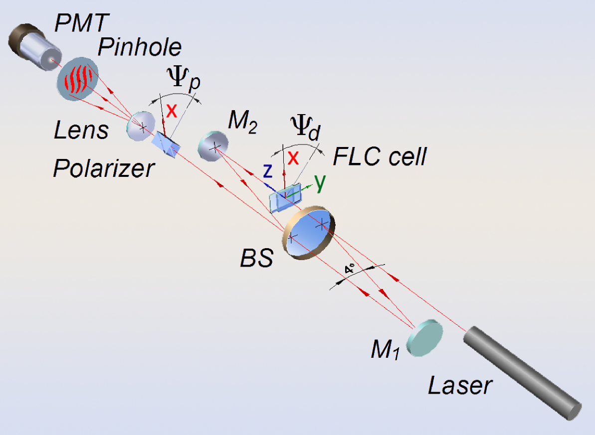
Figure 3: Experimental setup based on a Mach-Zehnder two-arm interferometer: BS is the beam splitter; M₁ and M₂ are the mirrors; PMT is the photomultiplier tube.

Electro-optical studies of DHFLC cells are typically carried out by measuring the transmittance of normally incident light passing through crossed polarizers. By contrast, our experimental setup shown in Fig. 3 is based on a Mach-Zehnder two-beam interferometer where the FLC cell is placed in the path of the sample beam.

A helium-neon laser with the wavelength of $632.8$ nm was used as a source of unpolarized light. A beam splitter (BS) divides a collimated unpolarized laser light into two beams, the reference and the sample beams, which, after reflection at the mirrors $M_{1}$ and $M_{2}$, are recombined at the semireflecting surface of the beam splitter (BS). The interfering beams emerging from the interferometer optionally pass through an output polarizer with the transmission axis azimuth $\psi_{p}$ and then are projected by the lens on to a screen with a pinhole. After passing the pinhole, light is collected by a photomultiplier (PMT) used in the linear regime as a photodetector.

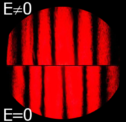
Figure 4: The interference fringes at $E\neq 0$ (top) and $E=0$ (bottom).

The interferometer was adjusted to obtain the fringes of equal thickness shown in Figs. 4 and 5. The period of the interference pattern was 120 times larger than the pinhole diameter and thus our measurements of the light intensity were performed with an accuracy less than 0.7%. In order to minimize the polarizing effects of Fresnel reflections, all the directions of incidence were close to the normal (deviations from the normal were less than $2^{\circ}$) so that the measured values of the degree of polarization of both beams were below $10^{-4}$.

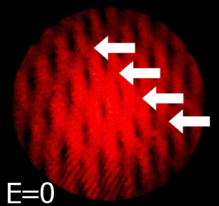
Figure 5: The interferogram obtained without the output polarizer shows the half-wave fringes indicated by arrows.

In order to facilitate data processing for signals registered by PMT, the mirrors $M_{1}$ and $M_{2}$ were fine tuned so as to bring the pinhole into coincidence with the position of an intensity minimum of the field-free interference pattern. The experimental results measured for triangular wave-form of driving voltage with the frequency $f=50$ Hz (the voltage applied across the DHFLC cell ranges from $-40$ V to $+40$ V) are presented in Figs. 6 and 7. These figures clearly indicate that the applied voltage results in modulation of the light intensity no matter whether the output wavefield passes through the polarizer or not. Another important effect is the electric field induced shift of the interference fringes which is illustrated in Fig. 4.

III Theory

Theoretically, the above findings can be interpreted in terms of the output beam written as the sum of the vector amplitudes

$$\mathbf{E}=\mathbf{E}_{s}+\mathbf{E}_{r}$$ (6)

representing the light transmitted through the FLC cell (the sample beam), $\mathbf{E}_{s}=\begin{pmatrix}E_{x}^{(s)}\\ E_{y}^{(s)}\end{pmatrix}$, and the reference beam, $\mathbf{E}_{r}=\begin{pmatrix}E_{x}^{(r)}\\ E_{y}^{(r)}\end{pmatrix}=\mathbf{T}_{r}\mathbf{E}_{0}=\mathrm{e}^{i\Phi_{0}}\mathbf{E}_{0}$, where $\mathbf{T}_{r}=\mathrm{e}^{i\Phi_{0}}\mathbf{I}_{2}$ and $\mathbf{I}_{2}$ is the $2\times 2$ unity matrix.

The vector amplitudes of incident and transmitted waves, $\mathbf{E}_{0}$ and $\mathbf{E}_{s}$, are related through the standard input-output relation

$$\mathbf{E}_{s}=\mathbf{T}_{s}\mathbf{E}_{0},$$ (7)

where $\mathbf{T}_{s}$ is the transmission matrix that, for the case of normal incidence, can be easily obtained from the general results of Refs. Kiselev et al. (2008); Kiselev and Chigrinov (2014) in the form:

$$\mathbf{T}_{s}=t_{+}\hat{\mathbf{d}}_{+}\otimes{\hat{\mathbf{d}}}^{\ast}_{+}+t_{-}\hat{\mathbf{d}}_{-}\otimes{\hat{\mathbf{d}}}^{\ast}_{-},$$ (8)

$$t_{\pm}=|t_{\pm}|\mathrm{e}^{i\Phi_{\pm}}=\frac{1-\rho_{\pm}^{2}}{1-\rho_{\pm}^{2}\exp(2in_{\pm}h)}\exp(in_{\pm}h),$$ (9)

where $\rho_{\pm}=(n_{\pm}-n_{\mathrm{m}})/(n_{\pm}+n_{\mathrm{m}})$ is the Fresnel reflection coefficient; $n_{\mathrm{m}}$ is the refractive index of the ambient medium; $h=k_{\mathrm{vac}}D$ is the thickness parameter; $k_{\mathrm{vac}}=\omega/c$ is the free-space wavenumber; and an asterisk will indicate complex conjugation. When the reflection coefficients, $\rho_{\pm}$, are small, the transmission coefficients, $t_{+}$ and $t_{-}$, can be approximated by the well-known formulas

$$t_{\pm}\approx\exp(i\Phi_{\pm}),\quad\Phi_{\pm}=n_{\pm}h.$$ (10)

and, in this reflectionless approximation, the transmission matrix is unitary.

The beam emerging from the interferometer and the incident light are characterized by the $2\times 2$ equal-time coherence matrices Mandel and Wolf (1995); Brosseau (1998), $\mathbf{M}$ and $\mathbf{M}_{0}$, with the elements $\mathbf{M}_{\alpha\beta}=\bigl{\langle}E_{\alpha}E_{\beta}^{\ast}\bigr{\rangle}$ and $\mathbf{M}_{\alpha\beta}^{(0)}=\bigl{\langle}E_{\alpha}^{(0)}\bigl{[}E_{\beta}^{(0)}\bigr{]}^{\ast}\bigr{\rangle}$, respectively. From the general relation linking these matrices $\mathbf{M}=\mathbf{T}\mathbf{M}_{0}\mathbf{T}^{\dagger}$, where $\mathbf{T}=\mathbf{T}_{s}+\mathbf{T}_{r}$ and a dagger will denote Hermitian conjugation, we have the coherence matrix of the output wavefield (6) given by

$$\mathbf{M}=\mathbf{M}_{r}+\mathbf{M}_{s}+\mathbf{M}_{i},\quad\mathbf{M}_{i}=\mathbf{T}_{s}\mathbf{M}_{0}\mathbf{T}_{r}^{\dagger}+\mathbf{T}_{r}\mathbf{M}_{0}\mathbf{T}_{s}^{\dagger},$$ (11)

where $\mathbf{M}_{r}=\mathbf{T}_{r}\mathbf{M}_{0}\mathbf{T}_{r}^{\dagger}=\mathbf{M}_{0}$ is the coherence matrix of the reference beam, $\mathbf{M}_{s}=\mathbf{T}_{s}\mathbf{M}_{0}\mathbf{T}_{s}^{\dagger}$ is the coherence matrix of the light transmitted through the DHFLC cell and $\mathbf{M}_{i}$ is the interference term.

For the case where the input light is unpolarized and its coherency matrix is proportional to the unity matrix, $\mathbf{M}_{0}=\dfrac{I_{0}}{2}\mathbf{I}_{2}\equiv\mathbf{M}_{u}$, the coherence matrix (11) takes the form:

$$\frac{1}{I_{0}}\mathbf{M}=\frac{m_{0}}{2}\mathbf{I}_{2}+\frac{m_{p}}{2}\begin{pmatrix}\cos 2\psi_{\mathrm{d}}&\sin 2\psi_{\mathrm{d}}\\ \sin 2\psi_{\mathrm{d}}&-\cos 2\psi_{\mathrm{d}}\end{pmatrix},$$ (12)

$$I/I_{0}\equiv m_{0}=1+\frac{|t_{+}|^{2}+|t_{-}|^{2}}{2}+\mathrm{Re}[\mathrm{e}^{-i\Phi_{0}}(t_{+}+t_{-})]$$

$$\approx 2\{1+\cos(\Phi-\Phi_{0})\cos(\Delta\Phi)\},$$ (13)

$$\Phi=(\Phi_{+}+\Phi_{-})/2,\quad\Delta\Phi=(\Phi_{+}-\Phi_{-})/2,$$ (14)

$$m_{p}=\frac{|t_{+}|^{2}-|t_{-}|^{2}}{2}+\mathrm{Re}[\mathrm{e}^{-i\Phi_{0}}(t_{+}-t_{-})]$$

$$\approx-2\sin(\Phi-\Phi_{0})\sin(\Delta\Phi),$$ (15)

where $I=\langle\mathbf{E}\cdot\mathbf{E}^{\ast}\rangle$ is the total intensity of the beams exiting the interferometer; $\Phi$ is the averaged phase shift; $2\Delta\Phi=(n_{+}-n_{-})h$ is the difference in optical path of the ordinary and extraordinary waves known as the phase retardation.

The approximate expressions for the intensity and polarization parameters, $m_{0}$ and $m_{p}$, are derived using the approximation given by Eq. (10). This is the case where the matrix $\mathbf{T}_{s}$ is unitary and, similar to the reference beam, the light field emerging from the FLC cell is unpolarized: $\mathbf{M}_{s}=\mathbf{M}_{r}=\mathbf{M}_{u}$. So, the only electric field dependent contribution to the coherence matrix of the total wavefield $\mathbf{M}$ (see Eq. (11)) comes from the interference term $\mathbf{M}_{i}$.

This term is responsible for the following two effects: (a) electrically induced modulation of the intensity described by Eq. (III); and (b) the total wavefield (6) is partially polarized with the degree of polarization $P=|m_{p}|/m_{0}$ and the Stokes parameters

$$(S_{1},S_{2},S_{3})=I_{0}m_{p}(\cos 2\psi_{\mathrm{d}},\sin 2\psi_{\mathrm{d}},0)\equiv I_{0}m_{p}\hat{\mathbf{s}}_{d}$$ (16)

varying with applied electric field. The latter, in particular, implies that the intensity of light that after the interferometer passes through a linear polarizer

$$I_{p}(\psi_{p})/I_{0}=[m_{0}+m_{p}\cos 2(\psi_{\mathrm{d}}-\psi_{p})]/2$$ (17)

depends on orientation of the polarizer transmission axis specified by the azimuthal angle $\psi_{p}$.

From (III), electric-field-induced modulation of the intensity does not depend on orientation of the optical axes (the azimuthal angle $\psi_{\mathrm{d}}$) and will occur even if the cell is optically isotropic and $\Phi_{+}=\Phi_{-}=\Phi$. Interestingly, this effect can be interpreted in terms of the Pancharatnam phase, $\Phi_{P}$.

This phase has a long history dating back to the original paper by Pancharatnam Pancharatnam (1956) (see also a collection of important papers Shapere and Wilczek (1989)) and can naturally be defined as the phase acquired by a light wave as it evolves along a path in the space of polarization states. In our case, the Pancharatnam phase is generated by evolution of mixed polarization states governed by the transmission matrix $\mathbf{T}_{s}(h)$ (a recent discussion of the Pancharatnam phase for pure and mixed states in optics can be found, e.g., in Hariharan (2005); Barberena et al. (2016)).

To be more specific, let us consider a partially polarized input beam with the degree of polarization equal to $P_{0}$ and the normalized coherency matrix $\rho_{0}=\mathbf{M}_{0}/I_{0}$ ($\mathrm{Tr}\rho_{0}=1$) which is known to play the role of the density matrix describing the mixed polarization state. This matrix can generally be expressed in terms of the eigenstates as follows

$$\rho_{0}=\frac{1+P_{0}}{2}\hat{\mathbf{f}}_{+}\otimes{\hat{\mathbf{f}}}^{\ast}_{+}+\frac{1-P_{0}}{2}\hat{\mathbf{f}}_{-}\otimes{\hat{\mathbf{f}}}^{\ast}_{-},$$ (18)

where the eigenpolarization vectors, $\hat{\mathbf{f}}_{+}$ and $\hat{\mathbf{f}}_{-}$, form the orthonormal basis that meets the orthogonality conditions: ${\hat{\mathbf{f}}}^{\ast}_{\mu}\cdot\hat{\mathbf{f}}_{\nu}=\delta_{\mu\nu}$ ($\delta_{\mu\nu}$ is the Kronecker delta). Similar to Eq. (16), the Stokes vector of the mixed state (18) can be written in the form:

$$(S_{1}^{(0)},S_{2}^{(0)},S_{3}^{(0)})=I_{0}P_{0}\hat{\mathbf{s}}_{0},$$ (19)

where $\hat{\mathbf{s}}_{0}$ is the normalized unit Stokes vector characterizing the partially polarized input wave.

In accordance with the interferometry based approach Sjöqvist et al. (2000); Tong et al. (2004), this is the interference part of the intensity, $I_{i}=\mathrm{Tr}\mathbf{M}_{i}$, determined by the interference term of the coherence matrix (11)

$$I_{i}/I_{0}=2\mathop{\rm Re}\nolimits[\mathrm{e}^{-i\Phi_{0}}F_{P}]=2V\cos(\Phi_{P}-\Phi_{0})$$ (20)

that gives the Pancharatnam phase, $\Phi_{P}$, and the visibility of the interference pattern, $V$. These are thus defined by the averaged transmission matrix through the general relation

$$F_{P}=\langle{\mathrm{T}_{s}(h)}\rangle_{0}\equiv\mathrm{Tr}[\mathbf{T}_{s}(h)\rho_{0}]=V\exp(i\Phi_{P}).$$ (21)

For the mixed state (18) and the transmission matrix (8), it is not difficult to derive the expression for $F_{P}$ which can be conveniently written in the following form:

$$F_{P}=[\tau_{+}+\tau_{-}P_{0}\cos\psi_{0}],\>\cos\psi_{0}=\hat{\mathbf{s}}_{0}\cdot\hat{\mathbf{s}}_{d},$$ (22)

$$\tau_{\pm}=(t_{+}\pm t_{-})/2.$$ (23)

In the case of unpolarized light and unitary transmission matrix [see Eq. (10)] where $P_{0}=0$ and $\tau_{+}\approx\cos(\Delta\Phi)\exp(i\Phi)$, the formulas for the Pancharatnam phase and the visibility assume the simplified form:

$$\Phi_{P}=\arg F_{P}\approx\begin{cases}\Phi,&\cos(\Delta\Phi)>0\\ \Phi+\pi,&\cos(\Delta\Phi)<0\\ \end{cases}$$ (24)

$$V=|F_{P}|\approx|\cos(\Delta\Phi)|.$$ (25)

It should be stressed that the phase $\Phi_{P}$ defined by the relations (21)–(23) is the total relative phase between the beams before and after the cell.

For unpolarized light with $P_{0}=0$, the Pancharatnam phase (24) is governed by the average of in-plane refractive indices: $(n_{+}+n_{-})/2$, whereas the visibility (25) is determined by the retardation phase $2\Delta\Phi$. The intensity of the interference pattern (III) can now be recast into the simple form

$$I=\mathrm{Tr}\,\mathbf{M}=2I_{0}[1+V\cos(\Phi_{P}-\Phi_{0})]$$ (26)

which is manifestly independent of optical axes orientation and shows that the electrically induced shift of the interferogram is solely dictated by the Pancharatnam phase.

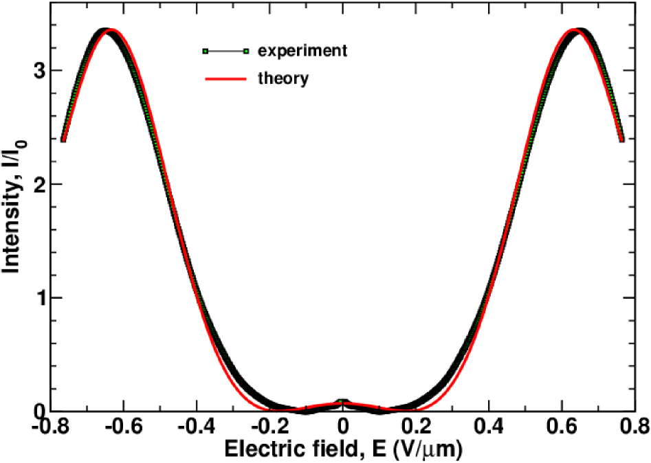
Figure 6: Intensity of output wavefield, $I/I_{0}$, as a function of the electric field for the DHFLC cell of thickness $D\approx 53$ $\mu$m filled with the FLC mixture FLC-624. Solid line represents the theoretical curve computed from (III) using the following parameters of the mixture: $n_{\perp}\approx 1.5$ is the ordinary refractive index, $n_{\parallel}\approx 1.71$ is the extraordinary refractive index, $\theta\approx 33^{\circ}$ is the smectic tilt angle, and $r_{2}\approx 1.03$ is the biaxiality ratio.

Note that the points where the visibility vanishes ($V=0$) represent the phase singularities where the Pancharatnam phase is undefined. In the observation plane, such singularity points may, under certain conditions, form curves that can be visualized as the zero visibility fringes. From (25), such fringes indicate the loci of the points where the phase retardation meets the condition of half-wave plates: $\cos(\Delta\Phi/2)=0$. So, these singularity lines might be called the half-wave fringes. Figure 5 shows the interferogram where such fringes arising from variations in cell thickness are easily discernible as zero-contrast stripes separating different areas of the interference fringes.

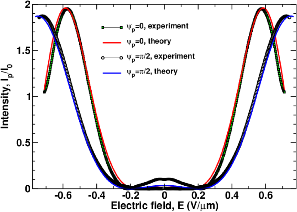
Figure 7: Intensity of output wavefield $I_{p}/I_{0}$, measured as a function of the electric field after the polarizer with the transmission axis oriented along ($\psi_{p}=0$) and perpendicular ($\psi_{p}=\pi/2$) to the helix axis. Solid lines represent the theoretical curves computed from (17) using the parameters listed in the caption of Fig. 6.

Formulas (III) and (17) in combination with the expressions for $n_{\pm}$ [see Eq. (41)] and $\psi_{\mathrm{d}}$ [see Eq. (46)] can now be used to fit the data on electric field dependence of the light intensity measured by the PMT and presented in Figs. 6 and 7. For this purpose, we assume that the FLC mixture is characterized by the parameters: $\epsilon_{\perp}\approx 2.22$ ($n_{\perp}\equiv n_{o}\approx 1.5$), $\epsilon_{\parallel}\approx 2.92$ ($n_{\parallel}\equiv n_{e}\approx 1.71$) and $\theta=33$^∘. Then the fitting gives the values of ratios: $P_{s}/\chi_{E}\approx 2.26$ V/$\mu$m and $r_{2}=\epsilon_{2}/\epsilon_{\perp}=1.03$ that are regarded as the fitting parameters. The theoretical curves are shown in Figs. 6 and 7. Interestingly, the value of the biaxiality ratio differs from unity and thus the optical anisotropy of the mixture appears to be weakly biaxial. Similar result was reported in our previous study Kotova et al. (2015).

IV Discussion and conclusion

In this paper, we have studied electric-field-induced modulation of unpolarized light in the DHFLC with subwavelength helix pitch using the experimental technique based on the Mach-Zehnder interferometer. Such modulation occurs under the action of the voltage applied across the cell and manifests itself in the electrically dependent shift and contrast of the interference pattern.

The shift and the visibility are found to be governed by the Pancharatnam phase and the phase retardation, respectively. The distinctive features of the electro-optic response in the regime of unpolarized illumination are: (a) insensitivity to the rotation of in-plane optical axes (this property was initially regarded as a requirement for pure phase modulation); and (b) modulation at subkiloherz operating frequencies (similar result was reported in Pozhidaev et al. (2014) for vertically aligned DHFLCs). So, modulation of unpolarized light driven by the orientational Kerr effect might be of considerable importance for applications in photonic devices such as deflectors, switchable gratings and wave-front correctors.

Our concluding remark concerns the Pancharatnam phase that, for the mixed polarization state (18), is given by formulas (21) and (22). The electrically induced shift of the interference fringes is naturally associated with this phase. We can also apply the approach of Refs. Sjöqvist et al. (2000); Tong et al. (2004) to derive the expression for the geometric phase $\Phi_{g}$  — the so-called Sjöqvist’s phase  – which is the part of $\Phi_{P}$ obtained by excluding the dynamical contribution. Such phase is an important characteristics which is determined solely by the geometry of the path in the space of polarization states.

In particular, when the transmission matrix is unitary [see Eq. (10)], it is rather straightforward to show that the geometric phase can be written in the following form:

$$\Phi_{g}=\arg(\mathop{\rm Re}\nolimits F_{g}+iP_{0}\mathop{\rm Im}\nolimits F_{g}),$$ (27)

$$F_{g}=[\cos(\Delta\Phi)+i\sin(\Delta\Phi)\cos\psi_{0}]\mathrm{e}^{-i\Delta\Phi\cos\psi_{0}}.$$ (28)

From Eqs. (27) and (28), it can be inferred that, similar to the visibility, $V=|F_{P}|$, the geometric phase $\Phi_{g}$ depends on the phase retardation $2\Delta\Phi$, and the angle between the unit Stokes vectors, $\hat{\mathbf{s}}_{0}$ and $\hat{\mathbf{s}}_{d}$, characterizing the input wave and the light linearly polarized along the optical axis $\hat{\mathbf{d}}_{+}$, respectively: $\cos\psi_{0}=\hat{\mathbf{s}}_{0}\cdot\hat{\mathbf{s}}_{d}$. It comes as no surprise that, for unpolarized incident light, the geometric phase (27) vanishes. Similar remark applies to the case of circular polarized light where $\cos\psi_{0}=0$. A more general case of non-unitary evolution requires a more sophisticated and comprehensive analysis of the electrically dependent geometric phases generated by DHFLC cells. Such analysis is beyond the scope of this paper and its results will be published elsewhere.

Appendix A Dielectric tensor of homogenized DHFLC cells

In this Appendix we recapitulate the key results on the effective dielectric tensor of the DHFLC cells. More details on these results can be found in Refs. Kiselev et al. (2011); Pozhidaev et al. (2013); Kiselev and Chigrinov (2014).

According to Ref. Kiselev et al. (2011), when the pitch-to-wavelength ratio $P/\lambda$ is sufficiently small, $P/\lambda<1$, the effective dielectric tensor

$$\boldsymbol{\varepsilon}_{\mathrm{eff}}=\begin{pmatrix}\epsilon_{xx}^{(\mathrm{eff})}&\epsilon_{xy}^{(\mathrm{eff})}&\epsilon_{xz}^{(\mathrm{eff})}\\ \epsilon_{yx}^{(\mathrm{eff})}&\epsilon_{yy}^{(\mathrm{eff})}&\epsilon_{yz}^{(\mathrm{eff})}\\ \epsilon_{zx}^{(\mathrm{eff})}&\epsilon_{zy}^{(\mathrm{eff})}&\epsilon_{zz}^{(\mathrm{eff})}\end{pmatrix}$$ (29)

can be expressed in terms of the averages over the pitch of the uniform lying distorted FLC helical structure

$$\eta_{zz}=\langle{\epsilon_{zz}^{-1}}\rangle=\epsilon_{0}^{-1}\langle{[1+u_{1}d_{z}^{2}+u_{2}p_{z}^{2}]^{-1}}\rangle,$$ (30)

$$\beta_{z\alpha}=\langle{\epsilon_{z\alpha}/\epsilon_{zz}}\rangle=\left\langle\frac{u_{1}d_{z}d_{\alpha}+u_{2}p_{z}p_{\alpha}}{1+u_{1}d_{z}^{2}+u_{2}p_{z}^{2}}\right\rangle,$$ (31)

where $\langle{\ldots}\rangle\equiv\langle{\ldots}\rangle_{\phi}=(2\pi)^{-1}\int_{0}^{2\pi}\ldots\mathrm{d}\phi$ and $\alpha\in\{x,y\}$, as follows:

$$\epsilon_{zz}^{(\mathrm{eff})}=1/\eta_{zz},\quad\epsilon_{z\alpha}^{(\mathrm{eff})}=\beta_{z\alpha}/\eta_{zz},$$

$$\epsilon_{\alpha\beta}^{(\mathrm{eff})}=\langle{\epsilon_{\alpha\beta}^{(P)}}\rangle+\beta_{z\alpha}\beta_{z\beta}/\eta_{zz},$$ (32)

where $\langle{\epsilon_{\alpha\beta}^{(P)}}\rangle$ are the components of the averaged tensor $\langle{\boldsymbol{\varepsilon}_{P}}\rangle$,

$$\langle{\epsilon_{\alpha\beta}^{(P)}}\rangle=\left\langle\epsilon_{\alpha\,\beta}-\frac{\epsilon_{\alpha\,z}\epsilon_{z\,\beta}}{\epsilon_{zz}}\right\rangle$$

$$=\epsilon_{0}\left\langle\delta_{\alpha\beta}+\frac{u_{1}d_{\alpha}d_{\beta}+u_{2}p_{\alpha}p_{\beta}+u_{1}u_{2}q_{\alpha}q_{\beta}}{1+u_{1}d_{z}^{2}+u_{2}p_{z}^{2}}\,\right\rangle,$$ (33)

$$q_{\alpha}=p_{z}d_{\alpha}-d_{z}p_{\alpha},\quad\alpha,\beta\in\{x,y\},$$ (34)

describing effective in-plane anisotropy that governs propagation of normally incident plane waves.

The general formulas (30)-(34) give the zeroth-order approximation for homogeneous models describing the optical properties of short-pitch DHFLCs. These formulas can be used to derive the effective optical tensor of the homogenized short-pitch DHFLC cell for both vertically and planar aligned FLC helices Kiselev et al. (2011); Pozhidaev et al. (2013); Kiselev and Chigrinov (2014).

We concentrate on the geometry of the uniform lying DHFLC helix shown in Fig. 1. For this geometry, the effective dielectric tensor can be written in the following form Kiselev and Chigrinov (2014):

$$\boldsymbol{\varepsilon}_{\mathrm{eff}}=\begin{pmatrix}\epsilon_{h}+\gamma_{xx}\alpha_{E}^{2}&\gamma_{xy}\alpha_{E}&0\\ \gamma_{xy}\alpha_{E},&\epsilon_{p}+\gamma_{yy}\alpha_{E}^{2}&0\\ 0&0&\epsilon_{p}-\gamma_{yy}\alpha_{E}^{2}\end{pmatrix},$$ (35)

where, following Ref. Pozhidaev et al. (2013), we have introduced the electric field parameter

$$\alpha_{E}=\chi_{E}E/P_{s}$$ (36)

proportional to the dielectric susceptibility of the Goldstone mode Carlsson et al. (1990); Urbanc et al. (1991): $\chi_{E}=\partial\langle{P_{z}}\rangle/\partial E$ with $P_{z}=P_{s}\cos\phi$.

The zero-field dielectric constants, $\epsilon_{h}$ and $\epsilon_{p}$, that enter the tensor (35) are given by

$$\epsilon_{h}/\epsilon_{\perp}=(n_{h}/n_{\perp})^{2}=r_{2}^{-1/2}\biggl{\{}\sqrt{r_{2}}$$

$$+u_{1}\cos^{2}\theta\left(\frac{r_{2}-1}{\sqrt{u}+\sqrt{r_{2}}}+u^{-1/2}\right)\biggr{\}},$$ (37a)

$$\epsilon_{p}/\epsilon_{\perp}=(n_{p}/n_{\perp})^{2}=\sqrt{r_{2}u},$$ (37b)

$$u=u_{1}\sin^{2}\theta+1.$$ (37c)

Similar results for the coupling coefficients $\gamma_{xx}$, $\gamma_{yy}$ and $\gamma_{xy}$ read

$$\gamma_{xx}/\epsilon_{\perp}=\frac{3\sqrt{r_{2}/u}}{(\sqrt{u}+\sqrt{r_{2}})^{2}}(u_{1}\cos\theta\sin\theta)^{2},$$ (38a)

$$\gamma_{yy}/\epsilon_{\perp}=\frac{3\sqrt{r_{2}u}}{(\sqrt{u}+\sqrt{r_{2}})^{2}}(u-r_{2}),$$ (38b)

$$\gamma_{xy}/\epsilon_{\perp}=\frac{2\sqrt{r_{2}}}{\sqrt{u}+\sqrt{r_{2}}}u_{1}\cos\theta\sin\theta.$$ (38c)

In Ref. Kiselev and Chigrinov (2014), the results (35)–(38c) were derived by using the averaging technique that allows high-order corrections to the dielectric tensor to be accurately estimated and improves agreement between the theory and the experimental data in the high-field region.

The dielectric tensor (35) is characterized by the three generally different principal values (eigenvalues) and the corresponding optical axes (eigenvectors) as follows

$$\boldsymbol{\varepsilon}_{\mathrm{eff}}=\epsilon_{z}\hat{\mathbf{z}}\otimes\hat{\mathbf{z}}+\epsilon_{+}\hat{\mathbf{d}}_{+}\otimes\hat{\mathbf{d}}_{+}+\epsilon_{-}\hat{\mathbf{d}}_{-}\otimes\hat{\mathbf{d}}_{-},$$ (39)

$$\epsilon_{z}=n_{z}^{\,2}=\epsilon_{zz}^{(\mathrm{eff})}=\epsilon_{p}-\gamma_{yy}\alpha_{E}^{2},$$ (40)

$$\epsilon_{\pm}=n_{\pm}^{\,2}=\bar{\epsilon}\pm\sqrt{[\Delta\epsilon]^{2}+[\gamma_{xy}\alpha_{E}]^{2}}$$ (41)

where

$$\bar{\epsilon}=(\epsilon_{xx}^{(\mathrm{eff})}+\epsilon_{yy}^{(\mathrm{eff})})/2=\bar{\epsilon}_{0}+(\gamma_{xx}+\gamma_{yy})\alpha_{E}^{2}/2,$$ (42)

$$\Delta\epsilon=(\epsilon_{xx}^{(\mathrm{eff})}-\epsilon_{yy}^{(\mathrm{eff})})/2=\Delta\epsilon_{0}+(\gamma_{xx}-\gamma_{yy})\alpha_{E}^{2}/2,$$ (43)

$$\bar{\epsilon}_{0}=(\epsilon_{h}+\epsilon_{p})/2,\>\Delta\epsilon_{0}=(\epsilon_{h}-\epsilon_{p})/2.$$ (44)

The in-plane optical axes are given by

$$\hat{\mathbf{d}}_{+}=\cos\psi_{d}\,\hat{\mathbf{x}}+\sin\psi_{d}\,\hat{\mathbf{y}},\quad\hat{\mathbf{d}}_{-}=\hat{\mathbf{z}}\times\hat{\mathbf{d}}_{+},$$ (45)

$$2\psi_{\mathrm{d}}=\arg[\Delta\epsilon+i\gamma_{xy}\alpha_{E}].$$ (46)

From Eq. (35), it is clear that the zero-field dielectric tensor is uniaxially anisotropic with the optical axis directed along the twisting axis $\hat{\mathbf{h}}=\hat{\mathbf{x}}$. The applied electric field changes the principal values (see Eqs. (40) and (41)) so that the electric-field-induced anisotropy is generally biaxial. In addition, the in-plane principal optical axes are rotated about the vector of electric field, $\mathbf{E}\parallel\hat{\mathbf{z}}$, by the angle $\psi_{\mathrm{d}}$ given in Eq. (46).

References

- Efron (1995) Uzi Efron, ed., Spatial Light Modulator Technology: Materials, Applications, and Devices (Marcell Dekker, NY, 1995) p. 665.
- Oswald and Pieranski (2006) Patrick Oswald and Pawel Pieranski, Smectic and Columnar Liquid Crystals: Concepts and Physical Properies Illustrated by Experiments, The Liquid Crystals Book Series (Taylor & Francis Group, London, 2006) p. 690.
- Love and Bhandari (1994) G. D. Love and R. Bhandari, “Optical properties of QHQ ferroelectric liquid crystal phase modulator,” Opt. Commun. 110, 475–478 (1994).
- Barnik et al. (1987) M. I. Barnik, V. A. Baikalov, V. G. Chigrinov, and E. P. Pozhidaev, “Electrooptics of a thin ferroeiectric smectic liquid crystal layer,” Mol. Cryst. Liq. Cryst. 143, 101–112 (1987).
- Pozhidaev et al. (1988) E. P. Pozhidaev, M. A. Osipov, V. G. Chigrinov, V. A. Baikalov, L. M. Blinov, and L. A. Beresnev, “Rotational viscosity of the smectic phase of ferroelectric liquid crystals,” Zh. Eksp. Teor. Fiz. 94, 125–132 (1988).
- Pozhidaev et al. (2013) Evgeny P. Pozhidaev, Alexei D. Kiselev, Abhishek Kumar Srivastava, Vladimir G. Chigrinov, Hoi-Sing Kwok, and Maxim V. Minchenko, “Orientational Kerr effect and phase modulation of light in deformed-helix ferroelectric liquid crystals with subwavelength pitch,” Phys. Rev. E 87, 052502 (2013).
- Pozhidaev et al. (2014) Evgeny P. Pozhidaev, Abhishek Kumar Srivastava, Alexei D. Kiselev, Vladimir G. Chigrinov, Valery V. Vashchenko, Alexander V. Krivoshey, Maxim V. Minchenko, and Hoi-Sing Kwok, “Enhanced orientational Kerr effect in vertically aligned deformed helix ferroelectric liquid crystals,” Optics Letters 39, 2900–2903 (2014).
- Blinov et al. (2005) L. M. Blinov, S. P. Palto, E. P. Pozhidaev, Yu. P. Bobylev, V. M. Shoshin, A. L. Andreev, F. V. Podgornov, and W. Haase, “High frequency hysteresis-free switching in thin layers smectic- ferroelectric liquid crystals,” Phys. Rev. E 71, 071715 (2005).
- Pozhidaev et al. (2012) Eugene Pozhidaev, Vladimir Chigrinov, Anatoli Murauski, Vadim Molkin, Du Tao, and Hoi-Sing Kwok, “V-shaped electro-optical mode based on deformed-helix ferroelectric liquid crystal with subwavelength pitch,” Journal of the SID 20, 273–278 (2012).
- Kotova et al. (2015) Svetlana P. Kotova, Sergey A. Samagin, Evgeny P. Pozhidaev, and Alexei D. Kiselev, “Light modulation in planar aligned short-pitch deformed-helix ferroelectric liquid crystals,” Phys. Rev. E 92, 062502 (2015).
- Kiselev et al. (2011) Alexei D. Kiselev, Eugene P. Pozhidaev, Vladimir G. Chigrinov, and Hoi-Sing Kwok, “Polarization-gratings approach to deformed-helix ferroelectric liquid crystals with subwavelength pitch,” Phys. Rev. E 83, 031703 (2011).
- Kiselev and Chigrinov (2014) Alexei D. Kiselev and Vladimir G. Chigrinov, “Optics of short-pitch deformed-helix ferroelectric liquid crystals: Symmetries, exceptional points, and polarization-resolved angular patterns,” Phys. Rev. E 90, 042504 (2014).
- Kiselev et al. (2008) A. D. Kiselev, R. G. Vovk, R. I. Egorov, and V. G. Chigrinov, “Polarization-resolved angular patterns of nematic liquid crystal cells: Topological events driven by incident light polarization,” Phys. Rev. A 78, 033815 (2008).
- Mandel and Wolf (1995) Leonard Mandel and Emil Wolf, Optical Coherence and Quantum Optics (Cambridge University Press, Cambridge, 1995) p. 1194.
- Brosseau (1998) Christian Brosseau, Fundamentals of Polarized Light: A Statistical Optics Approach (Wiley, New York, 1998) p. 424.
- Pancharatnam (1956) S. Pancharatnam, “Generalized theory of interference and its apllications,” The Proceedings of the Indian Academy of Sciences Sect. A 44, 247 (1956).
- Shapere and Wilczek (1989) Alfred Shapere and Frank Wilczek, Geometric Phases in Physics, Advanced Series in Mathematical Physics, Vol. 5 (World Scientific, Singapore, 1989) p. 509.
- Hariharan (2005) P. Hariharan, “The geometric phase,” Progress in Optics 48, 293–363 (2005).
- Barberena et al. (2016) D. Barberena, O. Ortíz, Y. Yugra, R. Caballero, and F. De Zela, “All-optical polarimetric generation of mixed-state single-photon geometric phases,” Phys. Rev. A 93, 013805 (2016).
- Sjöqvist et al. (2000) Erik Sjöqvist, Arun K. Pati, Artur Ekert, Jeeva S. Anandan, Marie Ericsson, Daniel K. L. Oi, and Vlatko Vedral, “Geometric phases for mixed states in interferometry,” Phys. Rev. Lett. 85, 2845–2849 (2000).
- Tong et al. (2004) D. M. Tong, E. Sjöqvist, L. C. Kwek, and C. H. Oh, “Kinematic approach to the mixed state geometric phase in nonunitary evolution,” Phys. Rev. Lett. 93, 080405 (2004).
- Carlsson et al. (1990) T. Carlsson, B. Žekš, C. Filipič, and A. Levstik, “Theoretical model of the frequency and temperature dependence of the complex dielectric constant of ferroelectric liquid crystals near the smectic- — smectic- phase transition,” Phys. Rev. A 42, 877–889 (1990).
- Urbanc et al. (1991) B. Urbanc, B. Žekš, and T. Carlsson, “Nonlinear effects in the dielectric response of ferroelectric liquid crystals,” Ferroelectrics 113, 219–230 (1991).