Short term prediction of extreme returns based on the recurrence interval analysis

Abstract

Being able to predict the occurrence of extreme returns is important in financial risk management. Using the distribution of recurrence intervals—the waiting time between consecutive extremes—we show that these extreme returns are predictable on the short term. Examining a range of different types of returns and thresholds we find that recurrence intervals follow a $q$-exponential distribution, which we then use to theoretically derive the hazard probability $W(\Delta t|t)$. Maximizing the usefulness of extreme forecasts to define an optimized hazard threshold, we indicates a financial extreme occurring within the next day when the hazard probability is greater than the optimized threshold. Both in-sample tests and out-of-sample predictions indicate that these forecasts are more accurate than a benchmark that ignores the predictive signals. This recurrence interval finding deepens our understanding of reoccurring extreme returns and can be applied to forecast extremes in risk management.

1 Introduction

Predicting such extreme financial events as market crashes, bank failures, and currency crises is of great importance to investors and policy markers because they destabilize the financial system and can greatly shrink asset value. Much research has been carried out in an attempt to detect the underlying vulnerabilities and the common precursors to financial extremes. A number of different models have been developed to predict the occurrence of financial distresses including those using probability (Martin, 1977; Canbas et al., 2005; Barrell et al., 2010; Tinoco and Wilson, 2013; Li and Wang, 2014; Lainà et al., 2015), signal approaches (Kaminsky et al., 1998; Edison, 2003; Duan and Bajona, 2008; Christensen and Li, 2014) and intelligence (Kumar and Ravi, 2007; Demyanyk and Hasan, 2010). A faster-than-exponential increase in price accompanied by accelerating price oscillations indicates the presence of bubbles (Sornette, 2003; Sornette and Cauwels, 2015). The behavior of these bubbles can be characterized using the log-period power-law singularity (LPPLS) model, which is capable of accurately forecasting a bubble’s tipping point (Sornette et al., 2009; Jiang et al., 2010; Sornette et al., 2015).

Recent research on the occurrence of financial extremes and on the market dynamics around financial crashes has enabled us to better forecast emerging financial crises. We can understand the occurrence pattern of extremes by determining the distribution of waiting times between consecutive financial extremes (the “recurrence intervals”) and charting the memory behavior within the occurring extremes. Bogachev and Bunde (2009); Jiang et al. (2016) built an early warning model of this waiting time distribution to predict the probability that extremes will occur within a given time period. Following a financial crisis the financial system gradually transitions back to a stasis (Bussiere and Fratzscher, 2006). This relaxation behavior following a financial market crash is similar to the aftershocks following an earthquake (Lillo and Mantegna, 2003; Petersen et al., 2010). Sornette (2003) indicates that a possible theoretical explanation for bursts of speculating bubbles is a positive herding behavior of traders that causes local self-excited crashes (Gresnigt et al., 2015). This is in accordance with the phenomenon that extremes cluster and are interdependent. Gresnigt et al. (2015) show that approximately 76–85% of occurring extremes are triggered by other extremes, and they develop an early warning model that treats financial crashes as earthquakes and compute the probability that an extreme event will occur within a certain time period.

Here we extend the probabilistic framework for extreme returns presented in Jiang et al. (2016) to predict extremes by using the conditional probability of an future extreme event within a fixed time frame in which Type 1 and Type 2 errors are balanced in current market state. The contributions of our works are in four ways.

• We identify extremes by locating the threshold at the minimum KS value between the empirical and fitting distributions of the extreme values.

• We classify the returns as either extreme or non-extreme by quantifying the extreme threshold, and we assume that the extremes are independent. This simplifies the modeling and reduces the computational complexity when estimating parameters but provides an adequate performance when doing out-of-sample prediction.

• We define a hazard probability that is dependent on the distribution formula of recurrence intervals between extremes, and this translates the problem into finding a suitable distribution form for recurrence intervals. Unlike the Hawkes point process, our modeling framework is easy to implement.

• Instead of using a predefined threshold of hazard probability, we predict extremes when the hazard probability exceeds an optimized hazard threshold, obtained by maximizing a usefulness function that takes into account an investor’s preference for either Type 1 or Type 2 errors.

We organize the paper as follows. In Section 2 we present a brief review of recurrence interval analysis and early warning models. In Section 3 we provide the dataset. In Section 4 we describe the Model and Methods. In Section 5 we present the results of our recurrence interval analysis for different subperiods. In Section 6 we document and discuss the performance of our out-of-sample predictions. In Section 7 we present our conclusions.

2 Literature review

2.1 Recurrence intervals analysis

Recurrence intervals, defined as the time periods between consecutive extreme events, have been a topic of extensive research across many fields, financial markets in particular. The primary contribution of the published research is an understanding of the statistical regularities in recurrence intervals. The memory behavior in the underlying process strongly affects the distribution form of recurrence intervals (Chicheportiche and Chakraborti, 2013, 2014). The interval distribution is exponential if the process has no memory. Incorporating a long memory into the underlying process greatly alters the recurrence interval distribution. For example, the stretched exponential and Weibull recurrence interval distribution are analytically and numerically confirmed in a process with a long linear memory (Santhanam and Kantz, 2008). When a process has a long nonlinear memory (a multifractual process), the recurrence intervals are power-law distributed (Bogachev et al., 2007).

There is extensive literature that examines the empirical distribution of recurrence intervals in financial markets. The distribution form is found to be dependent on data source, data type, and data resolution. For example, recurrence interval distributions with a power-law tail are found in the daily volatilities in the Japanese market (Yamasaki et al., 2005), in the minute volatilities in the Korean (Lee et al., 2006) and Italian markets (Greco et al., 2008), in the daily returns in the US stock markets (Bogachev et al., 2007; Bogachev and Bunde, 2009), in the minute returns in the Chinese markets (Ren and Zhou, 2010a), and in the minute volume in the US (Li et al., 2011) and Chinese markets (Ren and Zhou, 2010b). In addition, stretched recurrence interval distributions are also observed in the financial volatility at different resolutions in a range of different markets (Wang and Wang, 2012; Xie et al., 2014; Jiang et al., 2016). The $q$-exponential distribution has also been observed in the recurrence intervals between losses in financial returns (Ludescher et al., 2011; Ludescher and Bunde, 2014), and the corresponding distribution in the Chinese stock index future market is a stretched exponential (Suo et al., 2015).

In addition to the inconsistent findings on the distribution of empirical recurrence intervals, the existence of scaling behaviors in the recurrence interval distribution for the extremes filtered by different thresholds is under debate. Analyzing the distribution of recurrence intervals has indicated that the extreme event filtering threshold should influence the recurrence interval distribution (Xie et al., 2014; Chicheportiche and Chakraborti, 2014; Suo et al., 2015; Jiang et al., 2016). This indication was supported when the estimated distributional parameters were found to be strongly dependent on the thresholds when the recurrence intervals are fitted by such distribution functions as the stretched exponential distribution (Xie et al., 2014; Suo et al., 2015; Jiang et al., 2016) and the $q$-exponential distribution (Ludescher et al., 2011; Chicheportiche and Chakraborti, 2014; Jiang et al., 2016). Ludescher et al. (2011) and Ludescher and Bunde (2014) propose that the distribution of recurrence intervals depends only on the mean recurrence interval $\tau_{Q}$, and not on a specific asset or on the time resolution of the data.

Only a limited amount of research has used recurrence interval analysis to assess and manage risks in financial markets. An improved method for estimating the value at risk (VaR) based on the recurrence interval is significantly more accurate than traditional estimates based on the overall or local return distributions (Bogachev and Bunde, 2009; Ludescher et al., 2011). Another way of predicting extremes using statistics of recurrence intervals is also superior to the precursory pattern recognition technique when the underlying process is multifractal (Bogachev and Bunde, 2009). Defining a conditional loss probability as the inverse of the expected waiting time before observing another extreme determined by the latest recurrence interval, Ren and Zhou (2010a) finds that the risk of extreme loss events is high if the latest recurrence interval is long or short. In all of these studies, however, only in-sample tests are conducted, and a good performance in in-sample tests cannot ensure good results in out-of-sample tests. In contrast, Jiang et al. (2016) recently found that the extreme predicting method using recurrence interval analysis does provide good predictions in out-of-sample tests.

2.2 Early warning model of financial crisis

Such events as market crashes, currency crises, and bank failures are financial crisis in which the value of assets or the equity of financial institutions shrinks rapidly. Financial crises shock the real-world economy and can cause recessions or depressions if left unchecked. To reduce investor losses and shocks to the economy and to reduce financial turbulence, much effort has gone into predicting financial extremes. There is a plethora of literature on forecasting financial crises, especially currency crises and bank failures, and most of the research relies on the early warning model (EWM) (Kumar and Ravi, 2007; Demyanyk and Hasan, 2010). The EWM identifies the leading indicators of emerging financial problems and uses such techniques as logit (or probit) regressions and intelligence approaches to translate them into the hazard probability of crises occurring in the future, which is used as an early warning signal that indicates whether a crisis is imminent.

Compared to the vast EWM research predicting bank failures and currency crisis, early warning models to monitor stock markets and provide warning signals of market extremes have received little attention. The contributions of the existing literature are as follows.

A number of indicators are able to warn of incoming financial extremes. Coudert and Gex (2008) show that risk aversion indicators are useful in predicting stock market crises, but not currency crises. Chen (2009) finds that such macroeconomic indicators as yield curve spreads and inflation rates can be used to predict stock market recessions. Alessi and Detken (2011) show that a global measure of liquidity can predict asset price booms. Herwartz and Kholodilin (2014) show that the price-to-book ratio can predict emerging price bubbles. Li et al. (2015) show that such variables of index futures and options as the VIX, open interest, dollar volume, put option price, and put option effective spread can predict equity market crises. Chang et al. (2015) define the average value at risk (AVaRs) based on the ARMA-GARCH model with standard infinitely divisible innovations as an early warning indicator and find that AVARs can predict both extreme events and highly volatile markets. By constructing two investment networks based on the cross-border equity and a long-term debt securities portfolio, Joseph et al. (2014) identify two network-based indicators (algebraic connectivity and edge density) that could have predicted the 2008 global financial crisis. Minoiu et al. (2015) show that the interconnectedness in the global network of financial linkages could have predicted the financial crises that occurred during the 1978–2010 period.

Composite indices averaged from crisis-related variables have been proposed to predict financial crises. Oh et al. (2006) propose a daily financial condition indicator, market volatility, to determine whether a stock market is unstable or not. Kim et al. (2009) define and propose a stock market instability index based on the difference between the current market condition and the past conditions when the market was stable. Son et al. (2009) propose a model to predict stock market collapse that signals when a massive selling by global institutional investors occurs. Ahn et al. (2011) integrate all crisis-related variables into a monthly financial market condition indicator and find that by using a support vector machine the indicator can detect market crises. Yoon and Park (2014) use a market instability index to capture risk warning levels, quantify the instability level of the current market, and predict its future behavior.

There is a pattern of price trajectories that signals near-future market crashes. Sornette (2003) develops a log-periodic power law singularity (LPPLS) model for detecting bubbles by combining (i) the economic theory of rational expectation bubbles, (ii) the effect on the market of imitation and herding behaviors among investors and traders, and (iii) the mathematical and statistical physics of bifurcations and phase transitions. The faster-than-exponential (power law with finite-time singularity) increase in asset prices accompanied by accelerating oscillations is the main diagnostic that indicates bubbles (Sornette et al., 2009; Jiang et al., 2010; Sornette et al., 2015). Kurz-Kim (2012) also corroborate that the LPPLS pattern can be used as an early warning signal for market crashes. In addition, Yan and van Tuyll van Serooskerken (2015) convert the price series into networks using a visible graph alogorithm and use the degree-of-price network to measure the magnitude of the faster-than-exponential growth of stock prices, and to predict imminent financial extreme events. On average this indicator performs better than the LPPLS pattern-recognition indicator.

The patterns of financial crises are modeled to predict financial extreme events. Jiang et al. (2016) uncover the distribution pattern of waiting time between consecutive market extremes and use it to define a hazard probability that subsequent extremes will occur within a certain time period. They find that this hazard probability performs well in out-of-sample predictions. As an analogue to the seismic activity around earthquakes, Gresnigt et al. (2015) adopt an epidemic-type aftershock sequence model (a type of mutually self-exciting Hawkes point process) to capture the occurring dynamics of stock market crashes, which can serve as an early warning model for predicting the probability of medium-term crashes.

3 Data sets

We analyze the daily Dow Jones Industrial Average (DJIA) index from 16 February 1885 to 31 December 2015. The logarithmic return of the DJIA index over a time scale of one day is defined

$$r(t)=\ln I(t)-\ln I(t-1).$$ (1)

Figures 1(a) and 1(b) show plots of the logarithmic DJIA and its return, respectively. The DJIA index grows from 30.92 on 16 February 1885 to 17425.03 on 31 December 2015 with a total logarithmic return greater than 6. Although the index exhibits a rising trend throughout sample period, there are falling trends and range-bounds in different subperiods. Figure 1 shows six turbulent periods (highlighted in shadow), the Wall Street crash of 1929–1932, the oil crisis of 1973–1975, the Black Monday crash of 1987–1989, the dot-com bubble of 2000–2003, the subprime crisis 2007–2009, the 2008 financial crisis, and the European sovereign debt crisis 2011–2015.

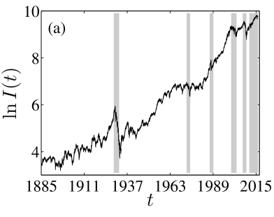
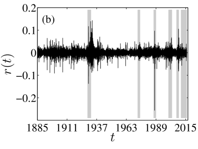
Figure 1: (color online). Plots of the logarithmic DJIA index $\ln I(t)$ and it’s difference, return $r(t)$. (a) $\ln I(t)$. (b) $r(t)$.

4 Model and Methods

4.1 Identifying extreme returns

An extreme value is usually defined as a peak above a threshold (POT) (Ren and Zhou, 2010b; Alessi and Detken, 2011; Christensen and Li, 2014; Sevim et al., 2014; Suo et al., 2015) that is $m$ times the sample standard deviation. The parameter $m$ is a predefined value (see a summary in Table 1 of Sevim et al. (2014)). Although identifying extreme events in terms of POT is widely applied in empirical analysis, the POT has drawbacks. A small $m$ value will produce many “extreme values,” not all of which are truly extreme, and a large $m$ value will indicate genuine extremes but not necessarily include all of them.

According to extreme value theory, the distribution of extreme values differs from that of non-extreme values. Finding the extreme values is equivalent to finding a group of data ($x\geq x_{t}$) that satisfies the extreme value distribution (Cumperayot and Kouwenberg, 2013)

$$G(x)=\left\{\begin{array}[]{ll}\exp\left[-(1+\gamma\frac{x-\mu}{\sigma})^{-1/\gamma}\right]&\textrm{for~{}~{}~{}~{} $\gamma\neq 0$}\\ \exp\left[-\exp(-\frac{x-\mu}{\sigma})\right]&\textrm{for~{}~{}~{}~{} $\gamma=0$}\end{array}\right.,$$ (2)

where $G(x)$ is the cumulative distribution of the generalized extreme value distribution, and $\mu$, $\sigma$, and $\gamma$ are location, scale, and shape parameters, respectively, and $x_{t}$ is the extreme value threshold. The inverse of the shape parameter $1/\gamma$ is simply the tail exponent of the sample distribution.

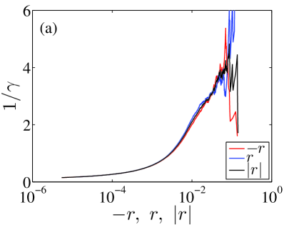
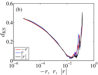
Figure 2: (color online). Determining the extreme value threshold $x_{t}$ for negative, positive, and absolute returns. (a) Plots of the tail exponents $1/\gamma$ as a function of the sorted returns. (b) Plots of the KS statistics $d_{\rm{KS}}$ with respect to the sorted returns. The KS statistics is defined as the maximum absolute difference between the empirical and fitting tail distributions.

We estimate the shape parameter $\gamma$ using the Hill estimator (Hill, 1975), which is a non-parametric method. For a given sample $\{x_{1},x_{2},\cdots,x_{n}\}$, we sort the data in ascending order,

$$x_{(1)}\leq x_{(2)}\leq\cdots\leq x_{(n)}.$$ (3)

The $\gamma$ value given by the Hill estimator is

$$\gamma=\frac{1}{k}\sum_{i=1}^{k}\left[\log x_{(n+1-k)}-\log x_{(k)}\right],$$ (4)

where $x_{k}$ corresponds to the extreme value threshold $x_{t}$ that will be determined.

One way to find threshold $x_{t}$ is by (i) estimating the value of $\gamma$ with respect to all possible values of $x_{t}$, and (ii) plotting $1/\gamma$ against $x_{t}$ to find a range of $x_{t}$ values within which the estimated $1/\gamma$ values are stable (Pozo and Amuedo-Dorantes, 2003; Reboredo et al., 2014). In practice, this “stable behavior” between $1/\gamma$ and $x_{k}$ is difficult to quantify. For example, Fig. 2(a) uses DJIA returns to illustrate the estimated $1/\gamma$ as a function of the sorted DJIA (negative, positive, and absolute) returns. The $1/\gamma$ values strongly fluctuate and there is no stable range. An alternative approach is to use KS statistics to measure the agreement between the empirical and fitting tail distributions. KS statistics quantify the maximum absolute difference between both distributions. The most suitable threshold $x_{t}$ is associated with the best fits to the tail distribution, which has the smallest KS statistical values (Clauset et al., 2009; Jiang et al., 2013). Figure 2(b) shows the plots of the KS statistics $d_{\rm{KS}}$ with respect to the sorted (negative, positive, and absolute) returns. The significant low point in each curve allows us to more easily determine the extreme value threshold $x_{t}$.

For sake of comparison, we also use the quantiles of 95%, 97.5%, and 99% to define the extremes. Definitions based on the quantile are common in the analysis of value-at-risk (VaR). Gresnigt et al. (2015) also define the 95% quantile of returns and the 95% quantile of negative returns as extremes and crashes.

4.2 Determining hazard probability

By taking into consideration only the time in which extremes occur, we base our prediction of extreme returns on the hazard probability $W(\Delta t|t)$, which measures the probability that following an extreme return occurring at $t$ time in the past there is an additional waiting time $\Delta t$ before another extreme return occurs. Sornette and Knopoff (1997) and Bogachev et al. (2007) theoretically derived the hazard probability $W(\Delta{t},t)$ using the distribution of recurrence intervals between extreme events,

$$W(\Delta{t}|t)=\frac{\int_{t}^{t+\Delta{t}}p(\tau){\rm{d}}\tau}{\int_{t}^{\infty}p(\tau){\rm{d}}\tau},$$ (5)

where $p(\tau)$ is the probability distribution of the recurring intervals. Once we have the distribution form of $p(\tau)$, the formula for $W(\Delta{t}|t)$ can be derived from Eq. (5).

Although the recurrence intervals of Poisson processes are exponentially distributed (Yamasaki et al., 2005; Bogachev et al., 2007; Chicheportiche and Chakraborti, 2014), which generates a constant hazard probability when $\Delta t$ is given, financial processes always exhibit such non-Poissonian characteristics as long-term dependence and multifractality in volatilities (Calvet and Fisher, 2002), medium-term dependence (e.g., momentum and contrarian behaviors (Chan et al., 1996; Shi et al., 2015)), and multiscaling behaviors in returns (Calvet and Fisher, 2002), which leads to that the recurrence intervals are no longer exponentially distributed, and that the derivation of the close distribution form for the recurrence intervals is obstructed (Chicheportiche and Chakraborti, 2013). The non-Poissonian features also result in a controversial situation in the empirical analysis of the distribution formula of recurrence intervals. For example, the reported distributions range from a power-law distribution with an exponential cutoff (Yamasaki et al., 2005; Lee et al., 2006; Greco et al., 2008; Ren and Zhou, 2010a) to a stretched exponential distribution (Wang and Wang, 2012; Suo et al., 2015; Jiang et al., 2016), from a $q$-exponential distribution (Ludescher et al., 2011; Ludescher and Bunde, 2014; Chicheportiche and Chakraborti, 2014) to a $q$-Weibull distribution (Reboredo et al., 2014). Here we employ three common functions to fit the recurrence interval distributions. The three formulas are the stretched exponential distribution,

$$p(\tau)=a\exp\left[-(b\tau)^{\mu}\right],$$ (6)

the $q$-exponential distribution,

$$p(\tau)=(2-q)\lambda[1+(q-1)\lambda\tau]^{-\frac{1}{q-1}},$$ (7)

and the Weibull distribution,

$$p(\tau)=\frac{\alpha}{\beta}\left(\frac{\tau}{\beta}\right)^{\alpha-1}\exp\left[-\left(\frac{\tau}{\beta}\right)^{\alpha}\right],$$ (8)

By putting the three probability distributions Eqs. (6)–(8) into Eq. (5), we obtain the hazard probability $W_{\rm{sE}}$ for the stretched exponential distribution,

$$W_{\rm{sE}}(\Delta t|t)=\frac{\frac{b\mu}{a}-\Gamma_{l}\left(\frac{1}{\mu},(bt)^{\mu}\right)-\Gamma_{u}\left(\frac{1}{\mu},[b(t+\Delta t)]^{\mu}\right)}{\Gamma_{u}\left(\frac{1}{\mu},(bt)^{\mu}\right)},$$ (9)

the hazard probability $W_{\rm{qE}}(\Delta t|t)$ for $q$-exponential distribution,

$$W_{\rm{qE}}(\Delta t|t)=1-\left[1+\frac{(q-1)\lambda\Delta t}{1+(q-1)\lambda t}\right]^{1-\frac{1}{q-1}},$$ (10)

and the hazard probability $W_{\rm{W}}(\Delta t|t)$ for Weibull distribution,

$$W_{\rm{W}}(\Delta t|t)=1-\exp\left[\left(\frac{t}{\beta}\right)^{\alpha}-\left(\frac{t+\Delta t}{\beta}\right)^{\alpha}\right],$$ (11)

where $\Gamma_{l}(s,x)$ and $\Gamma_{u}(s,x)$ are lower and upper incomplete gamma functions. For fixed $\Delta t$, all three hazard probabilities decrease as $t$ increases, which explains the clustering of extremes in financial returns and volatilities.

To use the hazard probability $W(\Delta t|t)$ to predict the extremes we must set a hazard threshold $w_{t}$ to trigger the early warning indicator of an approaching extreme event. If the hazard probability $W(\Delta t|t)$ is greater than the hazard threshold $w_{t}$, an alarm that an extreme return will occur during the next $\Delta t$ time is activated. The hazard threshold $w_{t}$ is not an arbitrary given value but—depending on the risk level preferences of investors—is optimized to balance between false alarms and not detecting events.

4.3 Evaluating predicting signals

The hazard probability $W(\Delta t|t)$ becomes a binary extreme forecast that equals one when $W(\Delta t|t)$ exceeds the hazard threshold $w_{t}$ and equals zero otherwise. When comparing the forecasted extremes with the actual events we see (i) correct predictions of an extreme return occurring, (ii) correct predictions of a non-extreme return occurring, (iii) missed events, and (iv) false alarms. By counting how many times each outcome occurs we can compute a range of evaluation measurements including the correct prediction rate, the false alarm rate, and the accuracy. Our primary interest here is correct prediction rate $D$ and false alarm rate $A$, which are defined as

$$D=\frac{n_{11}}{n_{01}+n_{11}},~{}~{}A=\frac{n_{10}}{n_{00}+n_{10}},$$ (12)

where $n_{11}$ is the number of extreme returns that are correctly predicted, $n_{00}$ the number of non-extreme returns that are correctly predicted, $n_{01}$ the number of missed events, and $n_{10}$ the number of false alarms. Following Gresnigt et al. (2015), we use the Hanssen-Kuiper skill score (KSS) to assess the validity of extreme forecasts. The KSS is the difference $D-A$ between the correct prediction rate and the false alarm rate. The KSS encompasses both missing occurrence errors and false alarms errors. Decreasing these two errors increases the value of KSS.

Our goal is to find a balanced signal for investors when they prefer either Type 1 and Type 2 errors and to take into account whether they use or discard the predictive signals. Following Alessi and Detken (2011) we define a loss function when a hazard probability threshold is added issue extreme forecasts,

$$L(\theta)=\theta(1-D)+(1-\theta)A,$$ (13)

where $1-D$ is the ratio of missing events (Type 1 errors) and $A$ is the ratio of false alarms (Type 2 errors). The parameter $\theta$ is the investor preference for avoiding either Type 1 or Type 2 errors (El-Shagi et al., 2013).

We further define the usefulness of extreme forecasts as

$$U(\theta)=\min(\theta,1-\theta)-L(\theta),$$ (14)

where $\min(\theta,1-\theta)$ is the loss faced by investors when they ignore the predictive signals, and $U(\theta)$ is the extent to which the extreme forecasting model offers better performance than no model at all (Betz et al., 2014). Extreme forecasts are useful when $U(\theta)>0$, which means that losses using the forecasts are lower than when the forecasts are ignored. The usefulness definition here ignores any influence from the data imbalance, i.e., that non-extreme events occur much more frequently than extreme events (Sarlin, 2013; Betz et al., 2014).

Given hazard probability $W(\Delta t|t)$, we need a hazard threshold $w_{t}$ that maximizes usefulness $U(\theta)$ (Duca and Peltonen, 2013; Babeckỳ et al., 2014; Betz et al., 2014). Christensen and Li (2014) optimizes the threshold by minimizing the noise-to-signal ratio $D/A$. When we optimize the usefulness there is a marginal rate of substitution between Type 1 and Type 2 errors, but this marginal rate is not clear in the optimization of the noise-to-signal ratio, and this can result in an unacceptable level of Type 1 and Type 2 errors (Alessi and Detken, 2011; El-Shagi et al., 2013; Babeckỳ et al., 2014).

4.4 Estimating distributional parameters

By introducing the stretched exponential function of Eq. (6) into the probability density function $\int_{0}^{+\infty}p(\tau){\rm{d}}\tau=1$, we obtain

$$\frac{a}{\mu b}\Gamma(\frac{1}{\mu})=1,$$ (15)

where $\Gamma(x)$ is the Gamma function. Podobnik et al. (2009) and Bogachev and Bunde (2009) describe the one-to-one correspondence between the average recurrence interval $\tau_{Q}$ and the percentage of extremes,

$$\tau_{Q}=\frac{1}{\int_{m}^{+\infty}p_{r}(r){\rm{d}}r}=\frac{1}{1-\int_{-\infty}^{m}p_{r}(r){\rm{d}}r}=\frac{1}{1-Q},$$ (16)

where $Q$ is the quantile that is used to define the extreme values. For this equation to be valid, the extremes must be positive. When extremes are negative, we convert them into positives by multiplying by $-1$. Chicheportiche and Chakraborti (2014) find that the average recurrence interval is universal irrespective of the dependence structure of the underlying process. From the definition of expectation, the average recurrence interval can also be written $\tau_{Q}=\int_{0}^{+\infty}\tau p(\tau){\rm{d}}\tau$. For the stretched exponential distribution, we have

$$\frac{a}{\mu b^{2}}\Gamma(\frac{2}{\mu})=\tau_{Q}.$$ (17)

By solving Eqs. (15) and (17) and using $\mu$ and $\tau_{Q}$ for the stretched exponential distribution, parameters $a$ and $b$ are

$$a=\frac{\mu\Gamma(2/\mu)}{\Gamma(1/\mu)^{2}\tau_{Q}},~{}~{}b=\frac{\Gamma(2/\mu)}{\Gamma(1/\mu)\tau_{Q}}.$$ (18)

This strategy reduces the number of estimated parameters from three to one.

The mean of the $q$-exponential distribution is $1/[\lambda(3-2q)]$. For there to be a mean, $q$ must be less than 3/2. Then the parameter $\lambda$ can be found using $q$ and $\tau_{Q}$,

$$\lambda=\frac{1}{\tau_{Q}(3-2q)}.$$ (19)

The expectation for the Weibull distribution is $\beta\Gamma(1+1/\alpha)$. Similarly, the $\beta$ can be expressed in terms of $\alpha$ and $\tau_{Q}$,

$$\beta=\frac{\tau_{Q}}{\Gamma(1+\frac{1}{\alpha})}.$$ (20)

We need to estimate only one parameter for the three distributions when they are used to fit the recurrence intervals. We adopt the maximum likelihood estimation (MLE) to estimate the distributional parameters. The logarithmic likelihood functions are the stretched exponential distribution

$$\ln L_{\rm{sE}}=n\ln a-\sum_{i=1}^{n}(b\tau_{i})^{\mu},$$ (21)

the $q$-exponential distribution

$$\ln L_{\rm{qE}}=n\ln[\lambda(2-q)]-\frac{1}{q-1}\sum_{i=1}^{n}\ln[1+(q-1)\lambda\tau_{i}],$$ (22)

and the Weibull distribution

$$\ln L_{\rm{W}}=n\ln\frac{\alpha}{\beta}+\sum_{i=1}^{n}\left[(\alpha-1)\ln\frac{\tau_{i}}{\beta}-\left(\frac{\tau_{i}}{\beta}\right)^{\alpha}\right],$$ (23)

in which $n$ is the number of recurrence intervals.

Taking the stretched exponential distribution as an example, the logarithmic likelihood function $\ln L_{\rm{sE}}$ is a one-variable function of $\mu$. Although usually we can solve the equation by taking the first order derivative of $\ln L_{\rm{sE}}$ with respect to $\mu$ to find the solution that maximizes the likelihood, here the analytical expression of the derivative of $\ln L_{\rm{sE}}$ with respect to $\mu$ is more difficult to obtain. We thus discretize $\mu$ in the $(0,1)$ range with a step of $10^{-6}$ and calculate the logarithmic likelihood function for each discrete value of $\mu$. The $\mu$ associated with the maximum value of $\ln L_{\rm{sE}}$ is the maximum likelihood estimation. In the same way we estimate the parameters $q\in(1,1.5)$ and $\alpha\in(0,1)$ for the $q$-exponential and Weibull distributions, respectively.

5 Recurrence interval analysis

In order to test the validity of our extreme-return-prediction model, we use the data before each turbulent period to calibrate the model and each turbulent period that follows for out-of-sample forecasting. We obtain six in-sample calibrating periods: 1885–1928, 1885–1972, 1885–1986, 1885–1999, 1885–2006, and 1885–2010 Their out-of-sample predicting periods are 1929–1932, 1973–1975, 1987–1989, 2000–2003, 2007–2009, and 2011–2015, respectively. In each in-sample calibrating period, we identify the extreme value threshold $x_{t}$ and extract the extreme values associated with $x_{t}$. We also locate the extreme values based on the quantile thresholds of 95%, 97.5%, and 99%. For each group of extreme values, we estimate the waiting time between consecutive extreme values, i.e., the recurrence interval. We take positive, negative, and absolute returns into account in our analysis because they may have connections with specific trading strategies. The investors holding long positions in the market are more sensitive to extreme negative returns and those holding short positions less sensitive.

Table 1 lists the recurrence intervals for different thresholds from different calibrating periods. Note that unlike the observations from the quantile threshold, the observations from the extreme value threshold do not increase monotonically as the calibration periods are expanded. The sharp decease in the number of recurrence intervals, for example from Panel B to Panel C for positive returns and from Panel C to Panel D for absolute returns, indicates that there is a dramatic increase in the extreme value threshold, suggesting that the market after 1973 became more volatile [see Fig. 1(b)]. The mean values of the recurrence interval are strongly influenced by the extreme values, as indicated by the large gap between the means and medians. Because the skewness is positive and the kurtosis is much greater than 3, the recurrence intervals also exhibit a right-skewed and fat-tailed distribution. This affirms the finding that the recurrence intervals obey a stretched exponential (Xie et al., 2014; Suo et al., 2015; Jiang et al., 2016) or a $q$-exponential distribution (Ludescher et al., 2011; Ludescher and Bunde, 2014; Chicheportiche and Chakraborti, 2014).

We see a significantly positive autocorrelation of lag 1 in the 95% column in Panel A and significant Ljung-Box Q statistics at the 0.01 level for the three types of returns. In addition the autocorrelation of lag 5 is also positive when returns are positive. This indicates that there are autocorrelations at short and long lags in the recurrence intervals at the 95% quantile threshold. In the 99% column the autocorrelations are close to 0 and the Ljung-Box Q statistics are insignificant for positive, negative, and absolute returns, suggesting that there are no correlations in the recurrence intervals. The results in both columns also show that the autocorrelation of recurrence intervals gradually decreases to insignificance when the quantile threshold increases from 95% to 99%, which is also seen in the columns of $x_{t}$ and 97.5% quantile. In Panels B through F, the autocorrelation coefficients at Lags 1 and 5 are all positive and statistically significant, indicating the presence of strong autocorrelations in the recurrence intervals. In addition, the Ljung-Box Q statistics of lag 30 are statistically significant at the 1% level, implying that significant autocorrelations are also prevalent when recurrence interval lags are longer. These results are supported by the long-memory behavior results of a detrended fluctuation analysis (DFA) of the recurrence intervals (Ren and Zhou, 2010b; Xie et al., 2014; Suo et al., 2015).

Table 1: Descriptive statistics of the recurrence intervals. This table reports number of observations (obsv), mean, median, standard deviation (stdev), skewness (skew), kurtosis (kurt), autocorrelation (rho), Ljung-Box Q test statistic (LBQ) of the return intervals between the extreme events, defined by the extreme value thresholds $x_{t}$ and quantile thresholds (95%, 97.5%, and 99%). The autocorrelation coefficients are calculated at lag 1 and 5. The Ljung-Box Q tests are conducted at lag 30. Panels A–F present the results from different in-sample calibrating periods.

		Negative return									Positive return									Absolute return
		$x_{t}$		95%		97.5%		99%			$x_{t}$		95%		97.5%		99%			$x_{t}$		95%		97.5%		99%
Panel A: in-sample calibrating period (1885 – 1928)
obsv		278.	0	652.	0	326.	0	130.	0		477.	0	652.	0	326.	0	130.	0		145.	0	652.	0	326.	0	130.	0
mean		46.	950	20.	0	40.	0	100.	0		27.	363	20.	0	40.	0	100.	0		90.	014	20.	0	40.	0	100.	0
median		12.	0	6.	500	11.	0	21.	0		12.	0	9.	0	16.	0	23.	500		12.	0	5.	0	6.	500	12.	0
stdev		91.	524	38.	122	78.	407	173.	978		44.	790	32.	100	78.	043	184.	695		182.	677	46.	844	94.	819	201.	517
skew		4.	713	6.	703	5.	131	3.	859		3.	782	4.	286	6.	067	3.	677		3.	704	9.	852	6.	000	3.	402
kurt		33.	706	80.	856	43.	300	24.	150		20.	607	27.	888	55.	805	20.	586		20.	540	157.	674	57.	471	16.	804
rho(1)		0.	120∗∗	0.	121∗∗∗	0.	140∗∗	0.	070		0.	257∗∗∗	0.	218∗∗∗	0.	081	$-$0.	028		0.	105	0.	143∗∗∗	0.	090	0.	082
rho(5)		$-$0.	064	0.	062	$-$0.	053	$-$0.	054		0.	083∗	0.	112∗∗∗	0.	142∗∗	$-$0.	086		$-$0.	040	0.	005	0.	041	$-$0.	058
Q(30)		48.	876∗∗	66.	026∗∗∗	36.	545	18.	890		131.	947∗∗∗	143.	181∗∗∗	41.	158∗	14.	910		18.	024	53.	899∗∗∗	30.	233	10.	549
Panel B: in-sample calibrating period (1885 – 1972)
obsv		2032.	0	1254.	0	627.	0	250.	0		1171.	0	1254.	0	627.	0	250.	0		2546.	0	1254.	0	627.	0	250.	0
mean		12.	349	20.	0	40.	0	100.	0		21.	430	20.	0	40.	0	100.	0		9.	856	20.	0	40.	0	100.	0
median		4.	0	5.	0	6.	0	8.	0		7.	0	7.	0	8.	0	12.	0		3.	0	3.	0	4.	0	6.	0
stdev		22.	546	43.	451	110.	804	251.	118		48.	351	43.	793	105.	520	281.	113		23.	928	59.	488	138.	074	276.	742
skew		5.	010	5.	606	7.	684	4.	409		8.	208	7.	289	6.	213	6.	072		7.	690	7.	306	7.	189	4.	007
kurt		41.	635	47.	837	84.	779	26.	219		110.	246	83.	273	50.	569	50.	613		89.	933	73.	524	65.	717	19.	536
rho(1)		0.	193∗∗∗	0.	295∗∗∗	0.	140∗∗∗	0.	532∗∗∗		0.	310∗∗∗	0.	303∗∗∗	0.	193∗∗∗	0.	215∗∗∗		0.	219∗∗∗	0.	194∗∗∗	0.	075∗	0.	311∗∗∗
rho(5)		0.	112∗∗∗	0.	098∗∗∗	0.	245∗∗∗	0.	090		0.	117∗∗∗	0.	106∗∗∗	0.	131∗∗∗	0.	309∗∗∗		0.	158∗∗∗	0.	085∗∗∗	0.	110∗∗∗	0.	407∗∗∗
Q(30)		843.	689∗∗∗	755.	150∗∗∗	206.	777∗∗∗	111.	717∗∗∗		753.	825∗∗∗	733.	710∗∗∗	432.	781∗∗∗	82.	437∗∗∗		1153.	606∗∗∗	585.	612∗∗∗	225.	441∗∗∗	110.	987∗∗∗
Panel C: in-sample calibrating period (1885 – 1986)
obsv		716.	0	1431.	0	715.	0	286.	0		1360.	0	1431.	0	715.	0	286.	0		2822.	0	1431.	0	715.	0	286.	0
mean		39.	989	20.	0	40.	0	100.	0		21.	053	20.	0	40.	0	100.	0		10.	146	20.	0	40.	0	100.	0
median		7.	0	5.	0	7.	0	8.	0		8.	0	7.	0	9.	0	12.	0		3.	0	4.	0	4.	0	6.	0
stdev		99.	845	43.	138	99.	905	253.	139		46.	590	44.	787	102.	571	272.	215		24.	320	58.	219	128.	684	270.	823
skew		5.	139	5.	507	5.	135	4.	222		8.	144	8.	664	6.	099	5.	977		7.	815	7.	182	6.	986	3.	832
kurt		34.	807	45.	983	34.	762	24.	000		111.	272	124.	207	50.	108	50.	643		93.	261	72.	012	66.	050	18.	315
rho(1)		0.	242∗∗∗	0.	284∗∗∗	0.	242∗∗∗	0.	565∗∗∗		0.	296∗∗∗	0.	259∗∗∗	0.	196∗∗∗	0.	221∗∗∗		0.	233∗∗∗	0.	205∗∗∗	0.	098∗∗∗	0.	213∗∗∗
rho(5)		0.	176∗∗∗	0.	117∗∗∗	0.	174∗∗∗	0.	307∗∗∗		0.	114∗∗∗	0.	130∗∗∗	0.	136∗∗∗	0.	271∗∗∗		0.	148∗∗∗	0.	075∗∗∗	0.	080∗∗	0.	237∗∗∗
Q(30)		276.	588∗∗∗	667.	824∗∗∗	277.	421∗∗∗	249.	183∗∗∗		791.	779∗∗∗	736.	976∗∗∗	450.	736∗∗∗	101.	007∗∗∗		1277.	446∗∗∗	597.	888∗∗∗	238.	276∗∗∗	182.	886∗∗∗
Panel D: in-sample calibrating period (1885 – 1999)
obsv		782.	0	1595.	0	797.	0	319.	0		1448.	0	1595.	0	797.	0	319.	0		1421.	0	1595.	0	797.	0	319.	0
mean		40.	816	20.	0	40.	0	100.	0		22.	043	20.	0	40.	0	100.	0		22.	462	20.	0	40.	0	100.	0
median		8.	0	6.	0	7.	0	8.	0		8.	0	8.	0	9.	0	13.	0		4.	0	4.	0	4.	0	5.	0
stdev		97.	920	41.	851	96.	353	248.	548		47.	351	43.	650	99.	684	270.	301		62.	523	56.	713	127.	547	270.	274
skew		5.	055	5.	511	5.	155	4.	210		7.	660	8.	550	6.	076	5.	746		6.	589	7.	148	7.	004	3.	903
kurt		34.	510	46.	938	35.	971	23.	986		99.	818	124.	073	50.	734	46.	911		60.	862	72.	525	65.	444	18.	877
rho(1)		0.	256∗∗∗	0.	278∗∗∗	0.	252∗∗∗	0.	548∗∗∗		0.	327∗∗∗	0.	259∗∗∗	0.	228∗∗∗	0.	199∗∗∗		0.	203∗∗∗	0.	214∗∗∗	0.	089∗∗	0.	206∗∗∗
rho(5)		0.	176∗∗∗	0.	131∗∗∗	0.	189∗∗∗	0.	273∗∗∗		0.	142∗∗∗	0.	139∗∗∗	0.	131∗∗∗	0.	326∗∗∗		0.	081∗∗∗	0.	082∗∗∗	0.	148∗∗∗	0.	203∗∗∗
Q(30)		277.	454∗∗∗	675.	904∗∗∗	303.	462∗∗∗	254.	647∗∗∗		849.	279∗∗∗	790.	724∗∗∗	467.	774∗∗∗	102.	416∗∗∗		677.	953∗∗∗	657.	786∗∗∗	195.	112∗∗∗	154.	916∗∗∗
Panel E: in-sample calibrating period (1885 – 2006)
obsv		834.	0	1683.	0	841.	0	336.	0		1539.	0	1683.	0	841.	0	336.	0		1518.	0	1683.	0	841.	0	336.	0
mean		40.	380	20.	0	40.	0	100.	0		21.	882	20.	0	40.	0	100.	0		22.	185	20.	0	40.	0	100.	0
median		8.	0	6.	0	8.	0	8.	0		8.	0	8.	0	9.	0	13.	0		4.	0	4.	0	4.	0	6.	0
stdev		95.	125	41.	361	94.	757	241.	773		46.	746	43.	235	102.	416	265.	009		60.	659	56.	179	124.	604	264.	232
skew		5.	213	5.	472	5.	240	4.	322		7.	580	8.	417	6.	467	5.	925		6.	795	7.	162	7.	148	3.	985
kurt		36.	645	46.	813	36.	980	25.	403		99.	236	122.	461	56.	734	50.	015		64.	680	72.	654	68.	333	19.	714
rho(1)		0.	258∗∗∗	0.	295∗∗∗	0.	254∗∗∗	0.	536∗∗∗		0.	337∗∗∗	0.	286∗∗∗	0.	282∗∗∗	0.	199∗∗∗		0.	206∗∗∗	0.	221∗∗∗	0.	102∗∗∗	0.	204∗∗∗
rho(5)		0.	178∗∗∗	0.	105∗∗∗	0.	193∗∗∗	0.	278∗∗∗		0.	151∗∗∗	0.	141∗∗∗	0.	081∗∗	0.	251∗∗∗		0.	083∗∗∗	0.	091∗∗∗	0.	058∗	0.	204∗∗∗
Q(30)		304.	082∗∗∗	873.	194∗∗∗	304.	969∗∗∗	260.	485∗∗∗		980.	303∗∗∗	875.	671∗∗∗	491.	718∗∗∗	106.	786∗∗∗		743.	033∗∗∗	673.	330∗∗∗	200.	311∗∗∗	158.	391∗∗∗
Panel F:in-sample calibrating period (1885 – 2010)
obsv		858.	0	1734.	0	867.	0	346.	0		924.	0	1734.	0	867.	0	346.	0		1540.	0	1734.	0	867.	0	346.	0
mean		40.	425	20.	0	40.	0	100.	0		37.	538	20.	0	40.	0	100.	0		22.	523	20.	0	40.	0	100.	0
median		7.	0	6.	0	7.	0	8.	0		9.	0	8.	0	9.	0	12.	0		4.	0	4.	0	4.	0	5.	0
stdev		111.	346	42.	218	109.	226	259.	435		97.	671	43.	424	104.	937	269.	598		68.	579	59.	451	132.	133	275.	164
skew		7.	095	5.	598	7.	081	4.	464		6.	397	8.	211	6.	287	5.	680		8.	097	7.	761	6.	888	3.	898
kurt		71.	630	49.	644	72.	329	26.	510		56.	115	117.	442	52.	915	46.	183		91.	999	83.	058	61.	436	18.	701
rho(1)		0.	146∗∗∗	0.	296∗∗∗	0.	161∗∗∗	0.	495∗∗∗		0.	308∗∗∗	0.	297∗∗∗	0.	302∗∗∗	0.	184∗∗∗		0.	218∗∗∗	0.	201∗∗∗	0.	112∗∗∗	0.	165∗∗∗
rho(5)		0.	174∗∗∗	0.	088∗∗∗	0.	132∗∗∗	0.	234∗∗∗		0.	084∗∗	0.	138∗∗∗	0.	191∗∗∗	0.	218∗∗∗		0.	113∗∗∗	0.	099∗∗∗	0.	057∗	0.	249∗∗∗
Q(30)		227.	668∗∗∗	877.	559∗∗∗	215.	488∗∗∗	223.	093∗∗∗		552.	569∗∗∗	994.	993∗∗∗	465.	599∗∗∗	99.	923∗∗∗		565.	484∗∗∗	613.	619∗∗∗	218.	575∗∗∗	146.	530∗∗∗

The recurrence intervals are fitted by the stretched exponential distribution, $q$-exponential distribution, and Weibull distribution in each in-sample calibrating period. Figure 3 shows the probability distribution of the recurrence intervals between the negative extreme events in the 99% quantile during the 1928 to 1985 in-sample calibrating period. The best fits to the three fitting distributions are also plotted as solid curves for comparison. Note that the stretched exponential distribution gives the best fit. Note also that the stretch exponential fits are most likely, which also agrees with the distribution of recurrence intervals between the negative and absolute extreme returns in the Chinese markets and the US markets (Wang et al., 2009; Ren and Zhou, 2010a; Xie et al., 2014; Suo et al., 2015). Because all the distribution curves are very similar, we do not show the recurrence intervals in other calibrating periods.

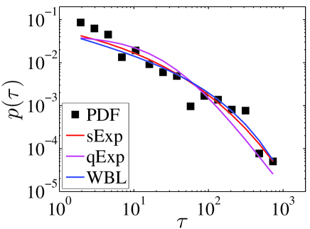
Figure 3: (color online). Distribution of the recurrence intervals. This figure presents the empirical distributions of the recurrence intervals between negative extreme returns in the quantile of 99% and the best fits to the three distributions, stretched exponential distribution, $q$-exponential distribution, and Weibull distribution. The analysis is performed in the period from 1885 to 1928.

Table 2 shows the estimated parameters of three fitting distributions of the recurrence intervals obtained from different return types and different thresholds. To assess the validity of the distributional fits, the logarithmic likelihoods are also listed. The likelihoods of the distribution with the maximum value are show in bold to indicate that the corresponding distribution gives the best fit. Panel A shows that the best recurrence interval fits transition from the $q$-exponential distribution to the stretched exponential distribution as the threshold is increased. This distribution transition behavior is also seen in the recurrence intervals in the minute volatilities in the Chinese stock markets (Jiang et al., 2016). Note that in Panels B–F the maximum likelihood comes from the $q$-exponential distribution for all the recurrence interval fits. Ludescher et al. (2011) and Ludescher and Bunde (2014) also found that the recurrence intervals between extreme loses are captured by the $q$-exponential distribution. The possible explanation for the lack of maximum likelihoods for the stretched exponential distribution in Panels B–F is that the 99% quantile threshold is not sufficiently large for a distribution transition from a $q$-exponential to a stretched exponential to occur.

Table 2 shows a monotonic trend between the estimated parameters and the quantile thresholds for each type of returns, such that $\mu$ and $\alpha$ decrease and $q$ increases as the quantile threshold increases. Our results support the dependence of the recurrence interval distribution on the quantile threshold (Xie et al., 2014; Chicheportiche and Chakraborti, 2014; Suo et al., 2015; Jiang et al., 2016). For the same quantile threshold and the same type of return, we also find that the estimated distributional parameters are close to each other in Panels B–F, which indicates that the recurrence interval distribution depends solely on the quantile (Ludescher et al., 2011; Ludescher and Bunde, 2014; Jiang et al., 2016).

Table 2: The estimated parameters and the maximum logarithmic likelihoods of the fits to the stretched exponential distribution, $q$-exponential distribution, and Weibull distribution for recurrence intervals. The likelihoods with the maximum value are highlighted in bold. The recurrence intervals are determined according to the extreme value thresholds $x_{t}$ and quantile thresholds (95%, 97.5%, and 99%) in the negative, positive, and absolute returns. Panels A–F present the results from different in-sample calibrating periods.

		Negative return									Positive return									Absolute return
		$x_{t}$		95%		97.5%		99%			$x_{t}$		95%		97.5%		99%			$x_{t}$		95%		97.5%		99%
Panel A: in-sample calibrating period (1885 – 1928)
$\mu$		0.	350	0.	461	0.	360	0.	280		0.	513	0.	573	0.	451	0.	307		0.	227	0.	383	0.	284	0.	215
$\ln L_{\rm{sE}}$		$-$1264.	269	$-$2496.	914	$-$1434.	225	$-$674.	465		$-$2000.	951	$-$2553.	728	$-$1473.	376	$-$680.	297		$-$700.	468	$-$2424.	402	$-$1365.	008	$-$634.	993
$q$		1.	408	1.	357	1.	405	1.	435		1.	316	1.	286	1.	345	1.	423		1.	461	1.	399	1.	443	1.	465
$\ln L_{\rm{qE}}$		$-$1266.	953	$-$2485.	817	$-$1434.	396	$-$684.	927		$-$1996.	519	$-$2544.	451	$-$1471.	303	$-$685.	261		$-$711.	080	$-$2411.	504	$-$1360.	696	$-$647.	154
$\alpha$		0.	625	0.	718	0.	634	0.	563		0.	757	0.	802	0.	708	0.	587		0.	498	0.	651	0.	556	0.	483
$\ln L_{\rm{W}}$		$-$1275.	718	$-$2523.	094	$-$1448.	428	$-$678.	027		$-$2014.	244	$-$2571.	295	$-$1483.	428	$-$684.	853		$-$707.	857	$-$2458.	188	$-$1386.	102	$-$641.	552
Panel B: in-sample calibrating period (1885 – 1972)
$\mu$		0.	512	0.	398	0.	294	0.	207		0.	433	0.	451	0.	315	0.	229		0.	452	0.	312	0.	230	0.	177
$\ln L_{\rm{sE}}$		$-$6870.	875	$-$4662.	711	$-$2602.	562	$-$1173.	240		$-$4501.	362	$-$4759.	720	$-$2654.	990	$-$1205.	945		$-$7787.	724	$-$4359.	017	$-$2384.	191	$-$1098.	368
$q$		1.	336	1.	396	1.	442	1.	473		1.	373	1.	363	1.	429	1.	464		1.	373	1.	438	1.	467	1.	483
$\ln L_{\rm{qE}}$		$-$6805.	955	$-$4610.	407	$-$2571.	429	$-$1165.	118		$-$4463.	297	$-$4718.	507	$-$2632.	444	$-$1200.	464		$-$7624.	907	$-$4248.	552	$-$2312.	401	$-$1081.	346
$\alpha$		0.	758	0.	663	0.	563	0.	465		0.	692	0.	706	0.	585	0.	492		0.	704	0.	577	0.	487	0.	422
$\ln L_{\rm{W}}$		$-$6957.	774	$-$4735.	734	$-$2650.	054	$-$1195.	844		$-$4559.	812	$-$4820.	370	$-$2696.	831	$-$1226.	002		$-$7951.	129	$-$4469.	435	$-$2453.	110	$-$1126.	514
Panel C: in-sample calibrating period (1885 – 1986)
$\mu$		0.	302	0.	409	0.	302	0.	208		0.	449	0.	463	0.	325	0.	229		0.	464	0.	322	0.	237	0.	179
$\ln L_{\rm{sE}}$		$-$3011.	043	$-$5359.	481	$-$3008.	233	$-$1348.	487		$-$5236.	811	$-$5455.	453	$-$3056.	744	$-$1382.	459		$-$8773.	031	$-$5036.	183	$-$2770.	080	$-$1272.	260
$q$		1.	437	1.	388	1.	437	1.	473		1.	362	1.	354	1.	424	1.	464		1.	365	1.	433	1.	465	1.	482
$\ln L_{\rm{qE}}$		$-$2980.	534	$-$5305.	811	$-$2978.	056	$-$1342.	692		$-$5195.	029	$-$5410.	298	$-$3035.	525	$-$1377.	135		$-$8608.	555	$-$4924.	461	$-$2701.	469	$-$1258.	164
$\alpha$		0.	571	0.	672	0.	571	0.	465		0.	705	0.	715	0.	594	0.	493		0.	714	0.	587	0.	496	0.	426
$\ln L_{\rm{W}}$		$-$3062.	519	$-$5438.	722	$-$3059.	523	$-$1373.	600		$-$5300.	912	$-$5521.	812	$-$3101.	494	$-$1405.	021		$-$8944.	445	$-$5155.	682	$-$2843.	627	$-$1302.	926
Panel D: in-sample calibrating period (1885 – 1999)
$\mu$		0.	307	0.	419	0.	308	0.	208		0.	457	0.	477	0.	335	0.	233		0.	314	0.	329	0.	241	0.	178
$\ln L_{\rm{sE}}$		$-$3325.	185	$-$6004.	925	$-$3375.	885	$-$1506.	977		$-$5657.	201	$-$6104.	959	$-$3430.	370	$-$1552.	323		$-$5155.	298	$-$5655.	759	$-$3115.	198	$-$1416.	369
$q$		1.	435	1.	382	1.	434	1.	472		1.	357	1.	345	1.	418	1.	462		1.	435	1.	429	1.	463	1.	482
$\ln L_{\rm{qE}}$		$-$3298.	423	$-$5953.	468	$-$3348.	336	$-$1501.	836		$-$5615.	392	$-$6055.	245	$-$3408.	686	$-$1548.	247		$-$5054.	298	$-$5540.	644	$-$3047.	366	$-$1403.	017
$\alpha$		0.	577	0.	681	0.	578	0.	467		0.	711	0.	726	0.	604	0.	498		0.	581	0.	595	0.	502	0.	424
$\ln L_{\rm{W}}$		$-$3378.	117	$-$6087.	515	$-$3429.	832	$-$1534.	442		$-$5722.	565	$-$6175.	819	$-$3477.	890	$-$1576.	590		$-$5271.	119	$-$5783.	800	$-$3193.	905	$-$1450.	209
Panel E: in-sample calibrating period (1885 – 2006)
$\mu$		0.	310	0.	422	0.	311	0.	214		0.	455	0.	472	0.	334	0.	235		0.	318	0.	331	0.	241	0.	181
$\ln L_{\rm{sE}}$		$-$3529.	464	$-$6339.	332	$-$3552.	077	$-$1598.	990		$-$5994.	090	$-$6429.	892	$-$3604.	772	$-$1636.	240		$-$5476.	112	$-$5959.	563	$-$3276.	784	$-$1502.	338
$q$		1.	434	1.	381	1.	433	1.	470		1.	359	1.	350	1.	419	1.	461		1.	434	1.	429	1.	463	1.	481
$\ln L_{\rm{qE}}$		$-$3498.	388	$-$6285.	001	$-$3519.	699	$-$1595.	926		$-$5947.	393	$-$6375.	880	$-$3577.	750	$-$1632.	522		$-$5364.	948	$-$5835.	504	$-$3203.	838	$-$1491.	093
$\alpha$		0.	582	0.	684	0.	582	0.	475		0.	710	0.	723	0.	603	0.	501		0.	585	0.	597	0.	503	0.	430
$\ln L_{\rm{W}}$		$-$3585.	778	$-$6425.	731	$-$3609.	157	$-$1626.	494		$-$6064.	641	$-$6506.	061	$-$3656.	471	$-$1661.	245		$-$5599.	175	$-$6094.	643	$-$3359.	717	$-$1536.	739
Panel F: in-sample calibrating period (1885 – 2010)
$\mu$		0.	305	0.	421	0.	308	0.	208		0.	338	0.	469	0.	333	0.	232		0.	312	0.	330	0.	237	0.	177
$\ln L_{\rm{sE}}$		$-$3616.	004	$-$6527.	378	$-$3651.	908	$-$1632.	635		$-$3910.	386	$-$6620.	877	$-$3712.	984	$-$1682.	142		$-$5558.	880	$-$6135.	844	$-$3356.	883	$-$1529.	646
$q$		1.	436	1.	382	1.	435	1.	472		1.	418	1.	352	1.	421	1.	462		1.	437	1.	429	1.	465	1.	483
$\ln L_{\rm{qE}}$		$-$3577.	687	$-$6465.	676	$-$3613.	537	$-$1625.	505		$-$3875.	292	$-$6562.	953	$-$3680.	043	$-$1677.	062		$-$5441.	337	$-$6002.	342	$-$3273.	580	$-$1512.	333
$\alpha$		0.	574	0.	682	0.	577	0.	466		0.	606	0.	720	0.	601	0.	497		0.	577	0.	595	0.	497	0.	422
$\ln L_{\rm{W}}$		$-$3678.	097	$-$6619.	216	$-$3714.	149	$-$1663.	022		$-$3969.	370	$-$6701.	078	$-$3768.	877	$-$1708.	772		$-$5688.	562	$-$6278.	192	$-$3446.	235	$-$1567.	267

When we obtain the distribution parameters, we can then find the theoretical curve of the hazard function for the $W_{\rm{sE}}$, $W_{\rm{qW}}$, and $W_{\rm{W}}$ by putting the parameters into the theoretical formula for hazard probability $W(\Delta t|t)$ given by Eqs. (9), (10), and (11) for the stretched exponential distribution, $q$-exponential distribution, and Weibull distribution, respectively. On the other hand, using Eq. (5) we can evaluate the empirical hazard function $W_{\rm{emp}}$,

$$W_{\rm{emp}}(\Delta t|t)=\frac{\#(t<\tau\leq t+\Delta t)}{\#(\tau>t)},$$ (24)

where the denominator $\#(\tau>t)$ is the number of recurrence intervals with values greater than $t$, and the numerator $\#(t<\tau\leq t+\Delta t)$ the number of recurrence intervals within the range of $(t,t+\Delta t]$.

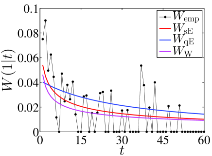
Figure 4: (color online). Plots of hazard probability $W(\Delta t|t)$ with $\Delta t=1$. The hazard events correspond to the extreme negative returns obtained from the quantile threshold of 99%. The analysis is performed in the period from 1885 to 1928.

Figure 4 shows a plot of the hazard probability $W(\Delta t|t)$ as a function of the elapsing time $t$ for the extreme negative returns obtained from the 99% quantile threshold when $\Delta t=1$. It shows the empirical hazard probability estimated from the real data (filled markers) and the analytical hazard probabilities obtained from the theoretical equations (solid curves). Note that although all the theoretical lines do not overlap on the same curve they all decrease with respect to the elapsing time $t$, as does the empirical hazard probability. The statistics are poor and the empirical hazard probability strongly oscillates, but for a given value of $t$ the analytical hazard probability values are comparable to those of the empirical hazard probability, suggesting that the analytical hazard probabilities agree with the empirical hazard probability. These decreasing patterns in the hazard probability are also seen in energy futures (Xie et al., 2014), spot index and index futures (Suo et al., 2015), and stock returns (Ren and Zhou, 2010a; Jiang et al., 2016), indicating that the probability of observing a follow-up extreme return decreases as time $t$ elapses. This reveals the existence of extreme return clustering and a potential dependent structure in the triggering processes of the extreme returns, which supports the argument that “many extreme price movements are triggered by previous extreme movements” and that “larger extremes occur more often after big events or frequent events than after tranquil periods” (Gresnigt et al., 2015). This is caused by the positive herding behavior of investors and the endogenous growth of instability in financial markets (Jiang et al., 2010; Gresnigt et al., 2015). Because the results are all similar, we do not show the hazard probabilities $W(\Delta t|t)$ for different thresholds and other types of return.

6 Predicting extreme returns

Using hazard probabilities and an optimized hazard threshold, we build a model to predict the occurrence of positive, negative, and absolute extreme returns in financial markets within a given time period. The hazard probabilities are specified by the distribution parameter of the recurrence intervals between extreme events in the return history. The indicators of incoming extreme events are generated when the hazard probability exceeds the optimized hazard threshold, and this maximizes the usefulness of these extreme forecasts. We perform out-of-sample tests to evaluate the predictive power of this extreme-return-prediction model as follows.

1. We mark extreme events according to a specified extreme value or quantile threshold during a given in-sample calibrating period.

2. Fitting the recurrence intervals between the marked extreme events, we estimate the stretched exponential distribution, $q$-exponential distribution, or Weibull distribution parameters.

3. Using the estimated distribution parameters in the in-sample calibrating period, we determine the hazard probability $W(\Delta t|t)$ and find the optimized hazard threshold $w_{t}$ by maximizing the usefulness $U(\theta)$.

4. Using the distribution parameters and optimized hazard threshold from the in-sample calibrating period, we forecast the indicators of incoming extreme events within time period $\Delta t$ and evaluate the forecasting signals.

To find the optimized hazard threshold, we vary the hazard threshold in $[0,1]$ to obtain all possible pairs of $(A,D)$. Plotting $A$ with respect to $D$, we obtain the well-known “receiver operator characteristic” (ROC) curve (Bogachev and Bunde, 2009). Using the ROC curve we measure the validity of the predicting power of early warning models. Figure 5 shows the ROC predictive curves of extreme negative returns for in-sample tests and out-of-sample tests. The in-sample (out-of-sample) period is from 1885 to 1928 (from 1929 to 1932). The diagonal line is a random guess. Note that the ROC curves of the three fitting distributions are overlap exactly on the same curve for in-sample and out-of-sample tests, suggesting that the results do not depend on the distribution formula used to fit the recurrence intervals. All ROC curves are above the random guess line, indicating that both in-sample and out-of-sample tests have a better predictive power than a random guess. Note also that the out-of-sample curves are lower than the in-sample curves, which confirms the observation that out-of-sample predictions are usually worse than in-sample tests (Lang and Schmidt, 2016). Because they all exhibit very similar patterns, we do not show the ROC curves obtained from different thresholds and different types of extreme returns.

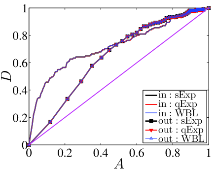
Figure 5: (color online). ROC curves of in-sample tests and out-of-sample predictions. The extreme returns correspond to the negative returns in the quantile of 99%. The in-sample period covers from 1885 to 1928. The out-of-sample period spans from 1929 to 1932.

Because all three fitting distributions give the same ROC curve, we evaluate only the in-sample and out-of-sample performance of the extreme return prediction model for the $q$-exponential distribution. We find the optimized hazard threshold, which maximizes the usefulness in the in-sample calibrating period, and estimate such performance measurements as the rate of correct predictions, the false alarm rate, the usefulness, and the KSS score during in-sample and out-of-sample periods. The results are shown in Table 3.

First, we observe that all usefulness $U$ values are positive except in the positive returns in the 97.5% quantile in Panel A and in the 95% quantile in Panel B, indicating that when missing-event and false-alarm errors are weighted equally our model provides more accurate results than the benchmark of ignoring the forecasting signals. Second, excluding the above two exceptions all KSS scores are greater than 0, which corresponds to random guessing, indicating that the rate of correct predictions exceeds that of false alarms. Third, note that in most of the results, the $U$ and KSS scores of in-sample performance are larger than those of out-of-sample performance, which is in consistent with the observation that out-of-sample predictions are inferior to the in-sample tests. We do find one exception in Panel E and nine exceptions in Panel F in which the out-of-sample predictions surpass the in-sample tests, and this indicates the predictive power of the testing model. The results also imply that the more data available for the in-sample tests, the better the performance of out-of-sample predictions, and this is further supported by the predictions during two recent turbulent periods, which were better than predictions during other periods. Fourth, note that the predictions of the extreme returns in the 99% quantile produce a lower false alarm rate and a higher correct prediction rate than those in the 95% and 97.5% quantiles, and this produces high usefulness and KSS scores. The results imply that the extreme events with a high quantile can be predicted more accurately. Table 1 shows the statistics of Ljung-Box Q tests that exhibit a decreasing pattern as quantile thresholds increase in all panels, indicating that increasing the quantile threshold could decrease the memory strength in the extremes. We neglect the potential dependence structure in the extreme series in our model because the larger the quantile threshold, the weaker the memory in extremes and the better the forecasting performance. Compared to the model based on the Hawkes processes (Gresnigt et al., 2015) our model has the advantage of fewer model parameters, easier estimating methods, and a faster prediction implementation.

Table 3: In-sample and out-of-sample performance of the extreme return predicting model. False alarm rates, correct predicting rate, usefulness, and KSS score is listed for in-sample tests and out-of-sample predictions. The predictions that out-of-sample performances are better than in-sample performances are highlighted in bold. The recurrence intervals are determined according to the extreme value thresholds $x_{t}$ and quantile thresholds (95%, 97.5%, and 99%) in the negative, positive, and absolute returns. Panels A–F present the results from different in-sample calibrating periods and out-of-sample predicting periods.

		Negative return									Positive return									Absolute return
		EVT		95%		97.5%		99%			EVT		95%		97.5%		99%			EVT		95%		97.5%		99%
Panel A: in-sample calibrating period (1885 – 1928) / out-of-sample predicting period (1929 – 1932)
in: $A$		0.	256	0.	319	0.	286	0.	228		0.	317	0.	382	0.	494	0.	263		0.	159	0.	207	0.	242	0.	142
out: $A$		0.	807	0.	814	0.	834	0.	895		0.	821	0.	862	0.	967	0.	773		0.	719	0.	699	0.	805	0.	721
in: $D$		0.	616	0.	623	0.	657	0.	626		0.	543	0.	602	0.	755	0.	656		0.	637	0.	582	0.	713	0.	626
out: $D$		0.	953	0.	949	0.	967	0.	980		0.	891	0.	898	0.	963	0.	963		0.	960	0.	935	0.	975	0.	958
in: $U$		0.	180	0.	152	0.	186	0.	199		0.	113	0.	110	0.	131	0.	197		0.	239	0.	187	0.	235	0.	242
out: $U$		0.	073	0.	068	0.	066	0.	042		0.	035	0.	018	$-$0.	002	0.	095		0.	121	0.	118	0.	085	0.	119
in: KSS		0.	361	0.	304	0.	372	0.	398		0.	226	0.	220	0.	261	0.	393		0.	478	0.	375	0.	470	0.	484
out: KSS		0.	146	0.	135	0.	133	0.	084		0.	069	0.	036	$-$0.	005	0.	190		0.	241	0.	236	0.	170	0.	238
Panel B: in-sample calibrating period (1885 – 1972) / out-of-sample predicting period (1973 – 1975)
in: $A$		0.	413	0.	332	0.	263	0.	120		0.	316	0.	337	0.	257	0.	191		0.	303	0.	170	0.	159	0.	075
out: $A$		0.	760	0.	634	0.	377	0.	111		0.	677	0.	676	0.	608	0.	361		0.	641	0.	360	0.	245	0.	042
in: $D$		0.	727	0.	729	0.	760	0.	725		0.	657	0.	664	0.	702	0.	757		0.	723	0.	700	0.	799	0.	737
out: $D$		0.	824	0.	750	0.	769	0.	250		0.	776	0.	782	0.	714	0.	692		0.	780	0.	671	0.	789	0.	667
in: $U$		0.	157	0.	199	0.	248	0.	302		0.	170	0.	163	0.	222	0.	283		0.	210	0.	265	0.	320	0.	331
out: $U$		0.	032	0.	058	0.	196	0.	069		0.	049	0.	053	0.	053	0.	166		0.	069	0.	155	0.	272	0.	312
in: KSS		0.	314	0.	397	0.	497	0.	605		0.	341	0.	327	0.	445	0.	566		0.	420	0.	531	0.	640	0.	663
out: KSS		0.	064	0.	116	0.	392	0.	139		0.	099	0.	106	0.	107	0.	331		0.	139	0.	311	0.	545	0.	624
Panel C: in-sample calibrating period (1885 – 1986) / out-of-sample predicting period (1987 – 1989)
in: $A$		0.	284	0.	342	0.	284	0.	193		0.	405	0.	362	0.	309	0.	191		0.	309	0.	177	0.	167	0.	099
out: $A$		0.	370	0.	512	0.	370	0.	291		0.	721	0.	688	0.	676	0.	394		0.	546	0.	336	0.	229	0.	205
in: $D$		0.	763	0.	717	0.	763	0.	780		0.	726	0.	675	0.	732	0.	753		0.	703	0.	680	0.	785	0.	749
out: $D$		0.	786	0.	667	0.	786	0.	750		0.	763	0.	683	0.	789	0.	733		0.	645	0.	662	0.	828	0.	733
in: $U$		0.	239	0.	187	0.	239	0.	294		0.	161	0.	157	0.	211	0.	281		0.	197	0.	252	0.	309	0.	325
out: $U$		0.	208	0.	077	0.	208	0.	230		0.	021	$-$0.	003	0.	057	0.	169		0.	050	0.	163	0.	299	0.	264
in: KSS		0.	479	0.	375	0.	478	0.	587		0.	321	0.	313	0.	423	0.	562		0.	394	0.	504	0.	618	0.	650
out: KSS		0.	416	0.	155	0.	416	0.	459		0.	042	$-$0.	005	0.	113	0.	339		0.	099	0.	325	0.	599	0.	529
Panel D: in-sample calibrating period (1885 – 1999) / out-of-sample predicting period (2000 – 2003)
in: $A$		0.	245	0.	350	0.	248	0.	140		0.	414	0.	370	0.	317	0.	185		0.	233	0.	181	0.	172	0.	105
out: $A$		0.	522	0.	690	0.	523	0.	330		0.	768	0.	702	0.	725	0.	461		0.	539	0.	463	0.	418	0.	278
in: $D$		0.	709	0.	707	0.	712	0.	725		0.	725	0.	669	0.	726	0.	734		0.	733	0.	669	0.	773	0.	747
out: $D$		0.	731	0.	821	0.	745	0.	533		0.	883	0.	820	0.	855	0.	769		0.	784	0.	664	0.	764	0.	700
in: $U$		0.	232	0.	178	0.	232	0.	292		0.	156	0.	149	0.	204	0.	275		0.	250	0.	244	0.	301	0.	321
out: $U$		0.	104	0.	065	0.	111	0.	102		0.	058	0.	059	0.	065	0.	154		0.	122	0.	100	0.	173	0.	211
in: KSS		0.	463	0.	357	0.	463	0.	585		0.	311	0.	298	0.	409	0.	549		0.	500	0.	487	0.	601	0.	642
out: KSS		0.	209	0.	130	0.	223	0.	204		0.	115	0.	118	0.	130	0.	308		0.	244	0.	201	0.	345	0.	422
Panel E: in-sample calibrating period (1885 – 2006) / out-of-sample predicting period (2007 – 2009)
in: $A$		0.	248	0.	351	0.	249	0.	144		0.	414	0.	367	0.	315	0.	186		0.	236	0.	258	0.	172	0.	107
out: $A$		0.	660	0.	711	0.	666	0.	333		0.	633	0.	603	0.	640	0.	423		0.	557	0.	616	0.	471	0.	175
in: $D$		0.	710	0.	708	0.	713	0.	715		0.	733	0.	678	0.	734	0.	730		0.	736	0.	746	0.	774	0.	742
out: $D$		0.	855	0.	902	0.	875	0.	900		0.	913	0.	869	0.	887	0.	933		0.	892	0.	911	0.	863	0.	969
in: $U$		0.	231	0.	179	0.	232	0.	286		0.	160	0.	155	0.	209	0.	272		0.	250	0.	244	0.	301	0.	317
out: $U$		0.	097	0.	095	0.	104	0.	283		0.	140	0.	133	0.	124	0.	255		0.	168	0.	147	0.	196	0.	397
in: KSS		0.	462	0.	357	0.	463	0.	571		0.	319	0.	311	0.	419	0.	544		0.	500	0.	489	0.	603	0.	634
out: KSS		0.	195	0.	191	0.	209	0.	567		0.	279	0.	266	0.	247	0.	510		0.	335	0.	294	0.	392	0.	793
Panel F: in-sample calibrating period (1885 – 2010) / out-of-sample predicting period (2011 – 2015)
in: $A$		0.	258	0.	350	0.	254	0.	140		0.	326	0.	439	0.	312	0.	183		0.	230	0.	256	0.	169	0.	100
out: $A$		0.	180	0.	352	0.	174	0.	128		0.	229	0.	358	0.	229	0.	136		0.	155	0.	195	0.	112	0.	066
in: $D$		0.	729	0.	712	0.	725	0.	726		0.	747	0.	752	0.	737	0.	738		0.	740	0.	751	0.	780	0.	758
out: $D$		0.	667	0.	636	0.	682	0.	667		0.	682	0.	696	0.	682	0.	714		0.	737	0.	720	0.	842	0.	571
in: $U$		0.	235	0.	181	0.	235	0.	293		0.	211	0.	157	0.	213	0.	277		0.	255	0.	248	0.	306	0.	329
out: $U$		0.	243	0.	142	0.	254	0.	269		0.	227	0.	169	0.	227	0.	289		0.	291	0.	262	0.	365	0.	253
in: KSS		0.	470	0.	362	0.	471	0.	587		0.	421	0.	313	0.	426	0.	554		0.	510	0.	495	0.	611	0.	658
out: KSS		0.	486	0.	285	0.	508	0.	538		0.	453	0.	338	0.	453	0.	578		0.	582	0.	525	0.	730	0.	505

7 Conclusion

We have performed a recurrence interval analysis of financial extremes in the DJIA index during the period from 1885 to 2015. We determine the extreme returns according to a newly proposed extreme identifying approach, as well as quantile thresholds. With the extreme identifying approach we are able to locate the optimal extreme threshold associated with the minimum KS statistics of tail distributions. We find that the recurrence intervals, which are the periods of time between the successive extremes of different types of returns and thresholds, follow a $q$-exponential distribution. This allows us to analytically derive the hazard probability $W(\Delta t|t)$ that within the time interval $\Delta t$ since the last extreme event that occurred at time $t$ we will observe the next extreme event. The analytical $W(\Delta t|t)$ value agrees well with the empirical hazard probability estimated from real data.

Using the hazard probability, we develop an extreme-return-prediction model for forecasting imminent financial extreme events. When the hazard probability is greater than the hazard threshold, this model can warn when an extreme event is about to occur. The hazard threshold is obtained by maximizing the usefulness of extreme forecasts. Both in-sample tests and out-of-sample predictions reveal that the signals generated by our prediction model are better statistically than the benchmark of neglecting these signals and that the input distribution formula used to fit the recurrence intervals has no influence on the final outcome of our early warning model. Although in most cases the predictive performance of in-sample tests are better than that of out-of-sample predictions, expanding the in-sample calibrating period could yield out-of-sample predictions that are better than in-sample tests. In addition, increasing the extreme-extracting threshold could improve the predictive power of our model in both in-sample tests and out-of-sample predictions. Our results may shed new light the occurrence of extremes in financial markets and on the application of recurrence interval analysis to forecasting financial extremes.

Reference

References

- Ahn et al. (2011) Ahn, J. J., Oh, K. J., Kim, T. Y., Dong, H. K., 2011. Usefulness of support vector machine to develop an early warning system for financial crisis. Expert Sys. Appl. 28, 2966–2973.
- Alessi and Detken (2011) Alessi, L., Detken, C., 2011. Quasi real time early warning indicators for costly asset price boom/bust cycles: A role for global liquidity. Eur. J. Polit. Econ. 27, 520–533.
- Babeckỳ et al. (2014) Babeckỳ, J., Havránek, T., Matějŭ, J., Rusnák, M., Šmídková, K., Vašíček, B., 2014. Banking, debt, and currency crises in developed countries: Stylized facts and early warning indicators. J. Financ. Stab. 15, 1–17.
- Barrell et al. (2010) Barrell, R., Davis, E. P., Karim, D., Liadze, I., 2010. Bank regulation, property prices and early warning systems for banking crises in OECD countries. J. Bank. Finance 34, 2255–2264.
- Betz et al. (2014) Betz, F., Oprică, S., Peltonen, T. A., Sarlin, P., 2014. Predicting distress in European banks. J. Bank. Finance 45, 225–241.
- Bogachev and Bunde (2009) Bogachev, M. I., Bunde, A., 2009. Improved risk estimation in multifractal records: Application to the value at risk in finance. Phys. Rev. E 80, 026131.
- Bogachev et al. (2007) Bogachev, M. I., Eichner, J. F., Bunde, A., 2007. Effect of nonlinear correlations on the statistics of return intervals in multifractal data sets. Phys. Rev. Lett. 99, 240601.
- Bussiere and Fratzscher (2006) Bussiere, M., Fratzscher, M., 2006. Towards a new early warning system of financial crises. J. Int. Money Finance 25 (953–973).
- Calvet and Fisher (2002) Calvet, L., Fisher, A., 2002. Multifractality in asset returns: Theory and evidence. Rev. Econ. Stat. 84, 381–406.
- Canbas et al. (2005) Canbas, S., Cabuk, A., Kilic, S. B., 2005. Prediction of commercial bank failure via multivariate statistical analysis of financial structures: The Turkish case. Eur. J. Oper. Res. 166, 528–546.
- Chan et al. (1996) Chan, L. K., Jegadeesh, N., Lakonishok, J., 1996. Momentum strategies. J. Finance 51 (5), 1681–1713.
- Chang et al. (2015) Chang, C.-C., Hu, T.-C., Kao, C.-F., Chang, Y.-C., 2015. Early warning signals using AVaRs of infinitely divisible GARCH models – evidence from stock index markets. Appl. Econ. 47, 4630–4652.
- Chen (2009) Chen, S.-S., 2009. Predicting the bear stock market: Macroeconomic variables as leading indicators. J. Bank. Finance 33, 211–223.
- Chicheportiche and Chakraborti (2013) Chicheportiche, R., Chakraborti, A., 2013. A model-free characterization of recurrences in stationary time series, http://arxiv.org/abs/1302.3704.
- Chicheportiche and Chakraborti (2014) Chicheportiche, R., Chakraborti, A., 2014. Copulas and time series with long-ranged dependencies. Phys. Rev. E 89, 042117.
- Christensen and Li (2014) Christensen, I., Li, F.-C., 2014. Predicting financial stress events: A signal extraction approach. J. Financ. Stab. 14, 54–65.
- Clauset et al. (2009) Clauset, A., Shalizi, C. R., Newman, M. E. J., 2009. Power-law distributions in empirical data. SIAM Rev. 51, 661–703.
- Coudert and Gex (2008) Coudert, V., Gex, M., 2008. Does risk aversion drive financial crises? Testing the predictive power of empirical indicators. J. Emp. Finance 15, 167–184.
- Cumperayot and Kouwenberg (2013) Cumperayot, P., Kouwenberg, R., 2013. Early warning systems for currency crises: A multivariate extreme value approach. J. Int. Money Finance 36, 151–171.
- Demyanyk and Hasan (2010) Demyanyk, Y., Hasan, I., 2010. Financial crises and bank failures: A review of prediction methods. Omega 38, 315–324.
- Duan and Bajona (2008) Duan, P., Bajona, C., 2008. China’s vulnerability to currency crisis: A KLR signals approach. China Econ. Rev. 19, 138–151.
- Duca and Peltonen (2013) Duca, M. L., Peltonen, T. A., 2013. Assessing systemic risks and predicting systemic events. J. Bank. Finance 37, 2183–2195.
- Edison (2003) Edison, H. J., 2003. Do indicators of financial crises work? An evaluation of an early warning system. Int. J. Fin. Econ., 11–53.
- El-Shagi et al. (2013) El-Shagi, M., Knedlik, T., von Schweinitz, G., 2013. Predicting financial crises: The (statistical) significance of the signals approach. J. Int. Money Finance 35, 76–103.
- Greco et al. (2008) Greco, A., Sorriso-Valvo, L., Carbone, V., Cidone, S., 2008. Waiting time distributions of the volatility in the Italian MIB30 index: Clustering or Poisson functions? Physica A 387, 4272–4284.
- Gresnigt et al. (2015) Gresnigt, F., Kole, E., Franses, P. H., 2015. Interpreting financial market crashes as earthquakes: A new early warning system for medium term crashes. J. Bank. Finance 56, 123–139.
- Herwartz and Kholodilin (2014) Herwartz, H., Kholodilin, K. A., 2014. In-sample and out-of-sample prediction of stock market bubbles: Cross-sectional evidence. J. Forecast. 33, 15–31.
- Hill (1975) Hill, B. M., 1975. A simple general approach to inference about the tail of a distribution. Ann. Statist. 3, 1163–1174.
- Jiang et al. (2016) Jiang, Z.-Q., Canabarro, A. A., Podobnik, B., Stanley, H. E., Zhou, W.-X., 2016. Early warning of large volatilities based on recurrence interval analysis in Chinese stock markets. To be appeared in Quant. Finance.
- Jiang et al. (2013) Jiang, Z.-Q., Xie, W.-J., Li, M.-X., Podobnik, B., Zhou, W.-X., Stanley, H. E., 2013. Calling patterns in human communication dynamics. Proc. Natl. Acad. Sci. U.S.A. 110 (5), 1600–1605.
- Jiang et al. (2010) Jiang, Z.-Q., Zhou, W.-X., Sornette, D., Woodard, R., Bastiaensen, K., Cauwels, P., 2010. Bubble diagnosis and prediction of the 2005-2007 and 2008-2009 Chinese stock market bubbles. J. Econ. Behav. Org. 74, 149–162.
- Joseph et al. (2014) Joseph, A. C., Joseph, S. E., Chen, G.-R., 2014. Cross-border portfolio investment networks and indicators for financial crises. Sci. Rep. 33, 3991.
- Kaminsky et al. (1998) Kaminsky, G., Lizondo, S., Reinhart, C. M., 1998. Leading indicators of currency crises. Staff Papers-International Monetary Fund, 1–48.
- Kim et al. (2009) Kim, D. H., Lee, S. J., Oh, K. J., Kim, T. Y., 2009. An early warning system for financial crisis using a stock market instability index. Expert Sys. 26, 260–273.
- Kumar and Ravi (2007) Kumar, P. R., Ravi, V., 2007. Bankruptcy prediction in banks and firms via statistical and intelligent techniques–a review. Eur. J. Oper. Res. 180, 1–28.
- Kurz-Kim (2012) Kurz-Kim, J.-R., 2012. Early warning indicator for financial crashes using the log periodic power law. Appl. Econ. Lett. 19, 1465–1469.
- Lainà et al. (2015) Lainà, P., Nyholm, J., Sarlin, P., 2015. Leading indicators of systemic banking crises: Finland in a panel of EU countries. Rev. Financial Econ. 24, 18–35.
- Lang and Schmidt (2016) Lang, M., Schmidt, P. G., 2016. The early warnings of banking crises: Interaction of broad liquidity and demand deposits. J. Int. Money Finance 61, 1–29.
- Lee et al. (2006) Lee, J. W., Lee, K. E., Rikvold, P. A., 2006. Waiting-time distribution for Korean stock-market index KOSPI. J. Korean Phys. Soc. 48, S123–S126.
- Li and Wang (2014) Li, S.-J., Wang, S., 2014. A financial early warning logit model and its efficiency verification approach. Knowledge-Based Systems 70, 78–87.
- Li et al. (2011) Li, W., Wang, F.-Z., Havlin, S., Stanley, H. E., 2011. Financial factor influence on scaling and memory of trading volume in stock market. Phys. Rev. E 84, 046112.
- Li et al. (2015) Li, W.-X., Chen, C. C.-S., French, J. J., 2015. Toward an early warning system of financial crises: What can index futures and options tell us? Quart. Rev. Econ. Finance 55, 87–99.
- Lillo and Mantegna (2003) Lillo, F., Mantegna, R. N., 2003. Power-law relaxation in a complex system: Omori law after a financial market crash. Phys. Rev. E 68, 016119.
- Ludescher and Bunde (2014) Ludescher, J., Bunde, A., 2014. Universal behavior of the interoccurrence times between losses in financial markets: Independence of the time resolution. Phys. Rev. E 90, 062809.
- Ludescher et al. (2011) Ludescher, J., Tsallis, C., Bunde, A., 2011. Universal behaviour of interoccurrence times between losses in financial markets: An analytical description. EPL (Europhys. Lett.) 95, 68002.
- Martin (1977) Martin, D., 1977. Early warning of bank failure: A logit regression approach. J. Bank. Finance 1, 249–276.
- Minoiu et al. (2015) Minoiu, C., C., K., Subrahmanian, V. S., Berea, A., 2015. Does financial connectedness predict crises? Quant. Finance 15, 607–624.
- Oh et al. (2006) Oh, K. J., Kim, T. Y., Kim, C., 2006. An early warning system for detection of financial crisis using financial market volatility. Expert Sys. 23, 83–98.
- Petersen et al. (2010) Petersen, A. M., Wang, F.-Z., Havlin, S., Stanley, H. E., 2010. Market dynamics immediately before and after financial shocks: Quantifying the Omori, productivity, and Bath laws. Phys. Rev. E 82, 036114.
- Podobnik et al. (2009) Podobnik, B., Horvatic, D., Petersen, A. M., Stanley, H. E., 2009. Cross-correlations between volume change and price change. Proc. Natl. Acad. Sci. U.S.A. 106, 22079–22084.
- Pozo and Amuedo-Dorantes (2003) Pozo, S., Amuedo-Dorantes, C., 2003. Statistical distributions and the identification of currency crises. J. Int. Money Finance 22, 591–609.
- Reboredo et al. (2014) Reboredo, J. C., Rivera-Castro, M. A., Machado de Assis, E., 2014. Power-law behaviour in time durations between extreme returns. Quant. Finance 14 (12), 2171–2183.
- Ren and Zhou (2010a) Ren, F., Zhou, W.-X., 2010a. Recurrence interval analysis of high-frequency financial returns and its application to risk estimation. New J. Phys. 12, 075030.
- Ren and Zhou (2010b) Ren, F., Zhou, W.-X., 2010b. Recurrence interval analysis of trading volumes. Phys. Rev. E 81, 066107.
- Santhanam and Kantz (2008) Santhanam, M. S., Kantz, H., 2008. Return interval distribution of extreme events and long-term memory. Phys. Rev. E 78, 051113.
- Sarlin (2013) Sarlin, P., 2013. On policymakers’ loss functions and the evaluation of early warning systems. Econ. Lett. 119, 1–7.
- Sevim et al. (2014) Sevim, C., Oztekin, A., Bali, O., Gumus, S., Guresen, E., 2014. Developing an early warning system to predict currency crises. Eur. J. Oper. Res. 237, 1095–1104.
- Shi et al. (2015) Shi, H.-L., Jiang, Z.-Q., Zhou, W.-X., 2015. Profitability of Contrarian Strategies in the Chinese Stock Market. PLos One 10, e0137892.
- Son et al. (2009) Son, I. S., Oh, K. J., Kim, T. Y., Kim, D. H., 2009. An early warning system for global institutional investors at emerging stock markets based on machine learning forecasting. Expert Sys. Appl. 36, 4951–4957.
- Sornette (2003) Sornette, D., 2003. Why Stock Markets Crash. Princeton University Press, Princeton.
- Sornette and Cauwels (2015) Sornette, D., Cauwels, P., 2015. Financial bubbles: mechanisms and diagnostics. Rev. Behav. Econ. 2, 279–305.
- Sornette et al. (2015) Sornette, D., Demos, G., Zhang, Q., Cauwels, P., Filimonov, V., Zhang, Q.-Z., 2015. Real-time prediction and post-mortem analysis of the Shanghai 2015 stock market bubble and crash. J. of Invest. Strategy. 4 (77–95).
- Sornette and Knopoff (1997) Sornette, D., Knopoff, L., 1997. The paradox of the expected time until the next earthquake. Bull. Seism. Soc. Am. 87, 789–798.
- Sornette et al. (2009) Sornette, D., Woodard, R., Zhou, W.-X., 2009. The 2006-2008 oil bubble: Evidence of speculation and prediction. Physica A 388 (8), 1571–1576.
- Suo et al. (2015) Suo, Y.-Y., Wang, D.-H., Li, S.-P., 2015. Risk estimation of csi 300 index spot and futures in china from a new perspective. Econ. Model. 49, 344–353.
- Tinoco and Wilson (2013) Tinoco, M. H., Wilson, N., 2013. Financial distress and bankruptcy prediction among listed companies using accounting, market and macroeconomic variables. Int. Rev. Financial Anal. 30, 394–419.
- Wang and Wang (2012) Wang, F., Wang, J., 2012. Statistical analysis and forecasting of return interval for SSE and model by lattice percolation system and neural network. Comput. Ind. Eng. 62, 198–205.
- Wang et al. (2009) Wang, F.-Z., Yamasaki, K., Havlin, S., Stanley, H. E., 2009. Multifactor analysis of multiscaling in volatility return intervals. Phys. Rev. E 79, 016103.
- Xie et al. (2014) Xie, W.-J., Jiang, Z.-Q., Zhou, W.-X., 2014. Extreme value statistics and recurrence intervals of NYMEX energy futures volatility. Econ. Model. 36, 8–17.
- Yamasaki et al. (2005) Yamasaki, K., Muchnik, L., Havlin, S., Bunde, A., Stanley, H. E., 2005. Scaling and memory in volatility return intervals in financial markets. Proc. Natl. Acad. Sci. U.S.A. 102, 9424–9428.
- Yan and van Tuyll van Serooskerken (2015) Yan, W.-F., van Tuyll van Serooskerken, E., 2015. Forecasting financial extremes: A network degree measure of super-exponential growth. PLoS One 10, e0128908.
- Yoon and Park (2014) Yoon, W. J., Park, K. S., 2014. A study on the market instability index and risk warning levels in early warning system for economic crisis. Digital Signal Process. 29, 35–44.