Abstract

A linearizable version of multidimensional system of $n$-wave type nonlinear PDEs is proposed. This system is derived using the spectral representation of its solution via the procedure similar to the dressing method for the ISTM-integrable nonlinear PDEs. The proposed system is shown to be completely integrable, particular solution is represented.

1 Introduction

The well known (2+1)-dimensional $n$-wave equation [1, 2] integrable by the inverse scattering transform method (ISTM) [3, 4, 5, 6, 7, 8, 9, 10]

$$[C^{(3)},v_{t_{2}}]-[C^{(2)},v_{t_{3}}]+C^{(2)}v_{t_{1}}C^{(3)}-C^{(3)}v_{t_{1}}C^{(2)}+[[C^{(3)},v],[C^{(2)},v]]=0$$ (1)

($C^{(i)}$ are constant diagonal matrices) gets a wide applicability in mathematical physics. In particular, it appears in multiple-scale expansions of various physical systems, where it describes the evolution of wave packets. Eq.(1) is the off-diagonal $N\times N$ ($N\geq 3$) first order partial differential equation (PDE) with quadratic nonlinearity of special form and $(N-1)N/2\geq 3$ different directional derivatives $\sum_{i=1}^{3}V^{(\alpha\beta)}_{i}\partial_{t_{i}}$ along the vectors $V^{(\alpha\beta)}$ with the coordinates

$$V^{(\alpha\beta)}_{1}=C^{(2)}_{\alpha}C^{(3)}_{\beta}-C^{(3)}_{\alpha}C^{(2)}_{\beta},\;\;V^{(\alpha\beta)}_{2}=C^{(3)}_{\alpha}-C^{(3)}_{\beta},\;\;V^{(\alpha\beta)}_{3}=C^{(2)}_{\beta}-C^{(2)}_{\alpha}.$$ (2)

However, its natural higher dimensional generalization is not integrable. An example of (partially) integrable multidimensional generalization of eq. (1) has a significantly deformed structure. One of its version possessing the periodic lump solution is found in [11].

The nonlinear PDE discussed in this paper reads (written in components)

$$\sum_{m=1}^{3}Z^{(m)}_{\alpha\beta}(v^{(lj)}_{\alpha\beta})_{t_{m}}+\sum_{n=1}^{2}T^{(n)}_{\alpha\beta}(v^{(lj)}_{\alpha\beta})_{x_{n}}-\sum_{k=1}^{2}\sum_{\gamma=1}^{N}a^{(k)}_{\alpha\gamma\beta}(v^{(lk)}_{\alpha\gamma}v^{(0j)}_{\gamma\beta}-v^{(l0)}_{\alpha\gamma}v^{(kj)}_{\gamma\beta})=0,$$ (3)

$$l,j=0,1,2,\;\;\alpha,\beta=1,\dots,N.$$

Here $v^{(lj)}$ are $N\times N$ matrix fields and $Z^{(m)}_{\alpha\beta}$, $T^{(n)}_{\alpha\beta}$, $a^{(k)}_{\alpha\gamma\beta}$ are constant coefficients having a special structure shown below in eqs.(33-48). The structure of this equation differs from that of (2+1)-dimensional $n$-wave equation (1), in particular, it involves $6$ matrix fields $v^{(lj)}$ instead of the single one. Similar to eq.(1), eq.(3) has the quadratic nonlinearity and $N(N-1)/2\geq 3$ directional derivatives $\sum_{m=1}^{3}Z^{(m)}_{\alpha\beta}\partial_{t_{i}}+\sum_{n=1}^{2}T^{(n)}_{\alpha\beta}\partial_{x_{n}}$. Since we have the five-dimensional space of independent variables, there are five independent directional derivatives.

Although the formal identification of different $v^{(ij)}$ (more exactly, the reduction $v^{(ij)}=C^{(i)}v^{(00)}C^{(j)}$ with some constant diagonal matrices $C^{(i)}$, $i=1,2$) is admittable by the structure of eq.(3), such the reduction cuts the solution space drastically decreasing its dimensionality, so that the reduced system loses its complete integrability.

The feature of system (3) is that its linear limit ($v^{(ij)}\to w^{(ij)}$)

$$\sum_{m=1}^{3}Z^{(m)}_{\alpha\beta}(w^{(ij)}_{\alpha\beta})_{t_{m}}+\sum_{n=1}^{2}T^{(n)}_{\alpha\beta}(w^{(ij)}_{\alpha\beta})_{x_{n}}=0,$$ (4)

$$i,j=0,1,2,\;\;\alpha,\beta=1,\dots,N,$$

is the same for all $i,j$. Since eq. (3) is linearizable [12, 13, 14] its solutions are formally related to the solutions of the associated system of linear partial differential equations (PDEs) (4). Deriving this relation, we turn to the spectral representation of solution as an auxiliary tool, and find a spectral function $\Psi(\lambda,\mu)$ of two spectral parameters. We call the algorithm deriving $v^{(ij)}$ in terms of the associated spectral function $\Psi$ a dressing algorithm in analogy with the dressing algorithm for equations integrable by ISTM [6, 7, 8, 9].

Thus, the paper has the following structure. In Sec.2 we represent a particular dressing method which will be used for deriving the system of nonlinear PDEs (3). The supplemented algebraic-differential relations among the fields of this system are derived in Sec.3. Solution space to system (3) is discussed in Sec.4, where an example of particular solution is given. Basic results are discussed in Sec.5.

2 Dressing method

2.1 Derivation of spectral equation

We consider the $N\times N$ matrix function $R(x;\lambda,\mu)$ depending on the two spectral parameters $\lambda$ and $\mu$ and set of auxiliary parameters $x=(x_{1},x_{2},\dots)$, which will be the independent variables of the nonlinear PDEs:

$$R(\lambda,\mu;x)=e^{\sum_{j=1}^{D}s^{(j)}(\lambda)x_{j}+\sum_{k}S^{(k)}(\lambda)t_{k}}R_{0}(\lambda,\mu)e^{-\sum_{j=1}^{D}s^{(j)}(\mu)x_{j}-\sum_{k}S^{(k)}(\mu)t_{k}}+r(\lambda)q(\mu),$$ (5)

where $r(\lambda)$ and $q(\mu)$ are some arbitrary diagonal functions of spectral parameters, $s^{(i)}$ are independent arbitrary diagonal functions of spectral parameter, while $S^{(m)}$ are linear combinations of $s^{(i)}$,

$$S^{(m)}(\lambda)=\sum_{i=1}^{D}A^{(mi)}s^{(i)}(\lambda),\;\;m=1,2,\dots,$$ (6)

with the diagonal constant matrices $A^{(mi)}$. In eq.(5), $R_{0}$ is some matrix functions of spectral parameters such that the operator $R(\lambda,\mu)$ is invertible. We refer to the inverse of $R$ as the spectral function $\Psi$:

$$\int d\Omega(\nu)R(x,\lambda,\nu)\Psi(x;\nu,\mu)\equiv R*\Psi=I\delta(\lambda-\mu),$$ (7)

where $\Omega(\nu)$ is some scalar measure on the plane of complex spectral parameter $\nu$, $I$ is the $N\times N$ identity operator. Differentiating $\Psi$ with respect to $x_{m}$ and taking into account its definition (7) and expression (5) for $R$ we obtain

$$\Psi_{x_{m}}(\lambda,\mu)=-\Psi(\lambda,\mu)s^{(m)}(\mu)+s^{(m)}(\lambda)\Psi(\lambda,\mu)+$$ (8)

$$\Big{(}\Psi(\lambda,\nu)s^{(m)}(\nu)\Big{)}*r(\nu)q(\tilde{\nu})*\Psi(\tilde{\nu},\mu)-\Psi(\lambda,\nu)*r(\nu)q(\tilde{\nu})*\Big{(}s^{(m)}(\tilde{\nu})\Psi(\tilde{\nu},\mu)\Big{)},$$

$$m=1,\dots,D.$$

$$\Psi_{t_{m}}(\lambda,\mu)=-\Psi(\lambda,\mu)S^{(m)}(\mu)+S^{(m)}(\lambda)\Psi(\lambda,\mu)+$$ (9)

$$\Big{(}\Psi(\lambda,\nu)S^{(m)}(\nu)\Big{)}*r(\nu)q(\tilde{\nu})*\Psi(\tilde{\nu},\mu)-\Psi(\lambda,\nu)*r(\nu)q(\tilde{\nu})*\Big{(}S^{(m)}(\tilde{\nu})\Psi(\tilde{\nu},\mu)\Big{)},$$

$$m=1,2\dots.$$

System (8,9) can be viewed as a system for the spectral function $\Psi$.

2.2 Derivation of system of nonlinear PDEs (3)

Now, applying the operators $(qs^{(i)})*$ and $*(s^{(j)}r)$, $i=0,1,2$ (with $s^{(0)}=1$) to eqs.(8) and (9) we obtain the system of nonlinear PDEs for the matrix fields

$$v^{(ij)}=(qs^{(i)})*\Psi*(s^{(j)}r),$$ (10)

$$v^{(in0j)}=(qs^{(i)}s^{(n)})*\Psi*(s^{(j)}r),\;\;\;v^{(i0nj)}=(qs^{(i)})*\Psi*(s^{(n)}s^{(j)}r),$$ (11)

$$v^{(i00j)}=v^{(i0j0)}=v^{(0i0j)}\equiv v^{(ij)}.$$

This system reads:

$$v^{(ij)}_{x_{m}}+v^{(i0mj)}-v^{(im0j)}-v^{(im)}v^{(0j)}+v^{(i0)}v^{(mj)}=0,$$ (12)

$$v^{(ij)}_{t_{m}}+\sum_{k=1}^{D}\Big{(}v^{(i0kj)}A^{(mk)}-A^{(mk)}v^{(ik0j)}\Big{)}-$$ (13)

$$\sum_{k=1}^{D}v^{(ik)}A^{(mk)}v^{(0j)}+v^{(i0)}\sum_{k=1}^{D}A^{(mk)}v^{(kj)}=0,$$

Using the proper combination of eqs.(12,13) we can eliminate the fields $v^{(i0mj)}$ and $v^{(im0j)}$ writing the system for the fields (10). For instance, taking $D=2$ we obtain the following nonlinear system (written in components):

$$\left|\begin{array}[]{ccccc}(e_{t_{1}}^{(ij)})_{\alpha\beta}&(e_{t_{2}}^{(ij)})_{\alpha\beta}&(e_{t_{3}}^{(ij)})_{\alpha\beta}&(e_{x_{1}}^{(ij)})_{\alpha\beta}&(e_{x_{2}}^{(ij)})_{\alpha\beta}\cr A^{(11)}_{\beta}&A^{(21)}_{\beta}&A^{(31)}_{\beta}&1&0\cr A^{(11)}_{\alpha}&A^{(21)}_{\alpha}&A^{(31)}_{\alpha}&1&0\cr A^{(12)}_{\beta}&A^{(22)}_{\beta}&A^{(32)}_{\beta}&0&1\cr A^{(12)}_{\alpha}&A^{(22)}_{\alpha}&A^{(32)}_{\alpha}&0&1\end{array}\right|=0$$ (19)

where we use the following notations:

$$e_{x_{m}}^{(ij)}:=v^{(ij)}_{x_{m}}-v^{(im)}v^{(0j)}+v^{(i0)}v^{(mj)},$$ (20)

$$e_{t_{m}}^{(ij)}:=v^{(ij)}_{t_{m}}-\sum_{k=1}^{2}v^{(ik)}A^{(mk)}v^{(0j)}+v^{(i0)}\sum_{k=1}^{2}A^{(mk)}v^{(kj)},$$

One can see that eq.(19) can be written as eq.(3) with

$$Z^{1}_{\alpha\beta}=\left|\begin{array}[]{cccc}A^{(21)}_{\beta}&A^{(31)}_{\beta}&1&0\cr A^{(21)}_{\alpha}&A^{(31)}_{\alpha}&1&0\cr A^{(22)}_{\beta}&A^{(32)}_{\beta}&0&1\cr A^{(22)}_{\alpha}&A^{(32)}_{\alpha}&0&1\end{array}\right|,\;\;Z^{2}_{\alpha\beta}=-\left|\begin{array}[]{cccc}A^{(11)}_{\beta}&A^{(31)}_{\beta}&1&0\cr A^{(11)}_{\alpha}&A^{(31)}_{\alpha}&1&0\cr A^{(12)}_{\beta}&A^{(32)}_{\beta}&0&1\cr A^{(12)}_{\alpha}&A^{(32)}_{\alpha}&0&1\end{array}\right|,\;\;Z^{3}_{\alpha\beta}=\left|\begin{array}[]{cccc}A^{(11)}_{\beta}&A^{(21)}_{\beta}&1&0\cr A^{(11)}_{\alpha}&A^{(21)}_{\alpha}&1&0\cr A^{(12)}_{\beta}&A^{(22)}_{\beta}&0&1\cr A^{(12)}_{\alpha}&A^{(22)}_{\alpha}&0&1\end{array}\right|,\;\;$$ (33)

$$T^{1}_{\alpha\beta}=\left|\begin{array}[]{cccc}A^{(11)}_{\beta}&A^{(21)}_{\beta}&A^{(31)}_{\beta}&0\cr A^{(11)}_{\alpha}&A^{(21)}_{\alpha}&A^{(31)}_{\alpha}&0\cr A^{(12)}_{\beta}&A^{(22)}_{\beta}&A^{(32)}_{\beta}&1\cr A^{(12)}_{\alpha}&A^{(22)}_{\alpha}&A^{(32)}_{\alpha}&1\end{array}\right|,\;\;T^{2}_{\alpha\beta}=\left|\begin{array}[]{cccc}A^{(11)}_{\beta}&A^{(21)}_{\beta}&A^{(31)}_{\beta}&1\cr A^{(11)}_{\alpha}&A^{(21)}_{\alpha}&A^{(31)}_{\alpha}&1\cr A^{(12)}_{\beta}&A^{(22)}_{\beta}&A^{(32)}_{\beta}&0\cr A^{(12)}_{\alpha}&A^{(22)}_{\alpha}&A^{(32)}_{\alpha}&0\end{array}\right|.$$ (42)

$$a^{(k)}_{\alpha\gamma\beta}=\left|\begin{array}[]{ccccc}A^{(1k)}_{\gamma}&A^{(2k)}_{\gamma}&A^{(3k)}_{\gamma}&\delta_{k1}&\delta_{k2}\cr A^{(11)}_{\beta}&A^{(21)}_{\beta}&A^{(31)}_{\beta}&1&0\cr A^{(11)}_{\alpha}&A^{(21)}_{\alpha}&A^{(31)}_{\alpha}&1&0\cr A^{(12)}_{\beta}&A^{(22)}_{\beta}&A^{(32)}_{\beta}&0&1\cr A^{(12)}_{\alpha}&A^{(22)}_{\alpha}&A^{(32)}_{\alpha}&0&1\end{array}\right|,\;\;k=1,2.$$ (48)

The structure of eq.(3) is similar to that of (2+1)-dimensional $n$-wave equation (1). In particular, it is off-diagonal and admits the reduction

$$x_{n}=i\xi_{n},\;\;t_{m}=i\tau_{m},\;\;,\;\;(v^{(lj)})^{+}=v^{(jl)},$$ (49)

$$i^{2}=-1,\;\;n=1,2,\;\;m=1,2,3,\;\;l,j=0,1,2.$$

Under this reduction, system (3) reads

$$i\sum_{m=1}^{3}Z^{(m)}_{\alpha\beta}(v^{(lj)}_{\alpha\beta})_{\tau_{m}}+i\sum_{n=1}^{2}T^{(n)}_{\alpha\beta}(v^{(lj)}_{\alpha\beta})_{\xi_{n}}+\sum_{k=1}^{2}\sum_{\gamma=1}^{N}a^{(k)}_{\alpha\gamma\beta}(v^{(lk)}_{\alpha\gamma}v^{(0j)}_{\gamma\beta}-v^{(l0)}_{\alpha\gamma}v^{(kj)}_{\gamma\beta})=0,$$

$$l,j=0,1,2,\;\;\alpha,\beta=1,\dots,N.$$

3 Supplemented algebraic-differential relations among functions $v^{(ij)}$

According to Sec.2, the off-diagonal elements of the matrix fields $v^{(ij)}$, $i,j=0,1,2$ satisfy system (3). In this section we show that there are natural supplemented algebraic-differential relations among these matrix fields, involving their diagonal elements. There are three families of such relations.

1. The first family is represented by the equations of systems (12,13) with $i=j=0$:

$$v^{(00)}_{x_{m}}+v^{(0m)}-v^{(m0)}-v^{(0m)}v^{(00)}+v^{(00)}v^{(m0)}=0,$$ (51)

$$v^{(00)}_{t_{m}}+\sum_{k=1}^{2}(v^{(0k)}A^{(mk)}-A^{(mk)}v^{(k0)})-\sum_{k=1}^{2}v^{(0k)}A^{(mk)}v^{(00)}+v^{(00)}\sum_{k=1}^{2}A^{(mk)}v^{(k0)}=0.$$

2. The second family is represented by the equations of systems (12,13) with $j=0$. Eliminating the fields $v^{(im00)}$ we write this family as

$$\left|\begin{array}[]{ccccc}(f_{t_{k}}^{(i0)})_{\alpha\beta}&(f_{x_{1}}^{(i0)})_{\alpha\beta}&(f_{x_{2}}^{(i0)})_{\alpha\beta}\cr A^{(k1)}_{\alpha}&1&0\cr A^{(k2)}_{\alpha}&0&1\end{array}\right|=0,\;\;k=1,2,3,$$ (55)

$$f_{x_{m}}^{(i0)}:=v^{(i0)}_{x_{m}}+v^{(im)}-v^{(im)}v^{(00)}+v^{(i0)}v^{(m0)},$$

$$f_{t_{m}}^{(i0)}:=v^{(i0)}_{t_{m}}+\sum_{k=1}^{2}v^{(ik)}A^{(mk)}-\sum_{k=1}^{2}v^{(ik)}A^{(mk)}v^{(00)}+v^{(i0)}\sum_{k=1}^{2}A^{(mk)}v^{(k0)},$$

3.The third family is represented by the equations of systems (12,13) with $i=0$. Eliminating the fields $v^{(00mj)}$ we write this family as

$$\left|\begin{array}[]{ccccc}(f_{t_{k}}^{(0j)})_{\alpha\beta}&(f_{x_{1}}^{(0j)})_{\alpha\beta}&(f_{x_{2}}^{(0j)})_{\alpha\beta}\cr A^{(k1)}_{\beta}&1&0\cr A^{(k2)}_{\beta}&0&1\cr\end{array}\right|=0,\;\;k=1,2,3,$$ (59)

$$f_{x_{m}}^{(0j)}:=v^{(0j)}_{x_{m}}-v^{(mj)}-v^{(0m)}v^{(0j)}+v^{(00)}v^{(mj)},$$

$$f_{t_{m}}^{(0j)}:=v^{(0j)}_{t_{m}}-\sum_{k=1}^{2}A^{(mk)}v^{(kj)}-\sum_{k=1}^{2}v^{(0k)}A^{(mk)}v^{(0j)}+v^{(00)}\sum_{k=1}^{2}A^{(mk)}v^{(kj)},$$

All relations (51-59) have the diagonal parts and involve diagonal elements of all matrix fields $v^{(ij)}$, $i,j=0,1,2$. However, we have to emphasize that the presence of these relations does not reduce the complete integrability of the system (3). This statement will be clarified in Sec.4

4 Solution space of system (3)

First of all, in this section we show the complete integrability of system (3). For this purpose we again turn to the spectral representation and derive the explicite form of the spectral function $\Psi$ and matrix fields $v^{(ij)}$.

4.1 Derivation of explicite formulas for $\Psi$ and $v^{(ij)}$

To construct the explicite form of $\Psi$ we have to invert the operator $R$, i.e., to solve the integral equation (7) for $\Psi$. It is remarkable that $\Psi$ can be constructed explicitly up to the invertibility of the integral operator $R_{0}$ independent on $x$- and $t$-variables. Substituting $R$ from (5) we rewrite eq.(7) as

$$\int\hat{R}_{0}(\lambda,\nu)\Psi(\nu,\mu)d\Omega(\nu)+r(\lambda)\chi(\mu)=\delta(\lambda-\mu),$$ (60)

where

$$\hat{R}_{0}(\lambda,\nu)=e^{\sum_{j=1}^{D}s^{(j)}(\lambda)x_{j}+\sum_{k}S^{(k)}(\lambda)t_{k}}R_{0}(\lambda,\mu)e^{-\sum_{j=1}^{D}s^{(j)}(\mu)x_{j}-\sum_{k}S^{(k)}(\lambda)t_{k}},\;\;$$ (61)

$$\chi(\mu)=\int q(\nu)\Psi(\nu,\mu)d\Omega(\nu).$$ (62)

Assuming the invertibility of $R_{0}(\lambda,\mu)$, we can write

$$\hat{R}_{0}^{-1}(\lambda,\mu)=e^{\sum_{j=1}^{D}s^{(j)}(\lambda)x_{j}+\sum_{k}S^{(k)}(\lambda)t_{k}}R_{0}^{-1}(\lambda,\mu)e^{-\sum_{j=1}^{D}s^{(j)}(\mu)x_{j}-\sum_{k}S^{(k)}(\mu)t_{k}},$$ (63)

where $R_{0}(\lambda,\nu)*R_{0}^{-1}(\nu,\mu)=\delta(\lambda-\mu)$. Then, applying $\hat{R}_{0}^{-1}*$, we can find $\Psi$ as

$$\Psi=\hat{R}_{0}^{-1}-\hat{R}_{0}^{-1}*r\chi.$$ (64)

The function $\chi$ in the rhs of this equation can be found applying $q*$ to eq.(64) and solving the obtained equation for $\chi$:

$$\chi=(1+w^{(00)})q*\hat{R}_{0}^{-1},$$ (65)

where we introduce the following notations:

$$w^{(ij)}=(qs^{(i)})*\hat{R}_{0}^{-1}*(s^{(j)}r),\;\;i,j=0,1,\dots,D,\;\;s^{(0)}=I_{N}.$$ (66)

Applying $(qs^{(i)})*$ and $*(s^{(j)}r)$ to eq.(64) we obtain:

$$v^{(ij)}=w^{(ij)}-w^{(i0)}(I+w^{(00)})^{-1}w^{(0j)}.$$ (67)

Obviously, each of the functions $w^{(ij)}$ is a solution of the appropriate linear PDE (4). Solutions $v^{(ij)}$ have no singularities if ${\mbox{det}}(I+w^{(00)})\neq 0$ for all $x_{i}$ and $t_{i}$ inside of the domain of our interest.

The conclusion regarding the complete integrability of system (3) follows from the fact that the function $R$ (61) has arbitrary dependence on $2D$ independent functions of spectral parameters $s^{(i)}(\lambda)$ and $s^{(i)}(\mu)$ thus providing arbitrary functions of $2D$ independent variables $x_{i}$ and $t_{i}$. This is a necessary requirement for complete integrability of the system of $(2D+1)$-dimensional PDEs. Obviously, the number of these arbitrary matrix functions of $(x,t)$-variables coincides with the number of fields $v^{(ij)}$ in system (3). In fact, these arbitrary functions are nothing but the fields $w^{(ij)}$ (66). By construction, they are independent functions having arbitrary dependence on $2D$ variables $x_{i}$ and $t_{i}$.

In addition, to satisfy the reduction (49), we shall impose the following constraints on the functions of spectral parameters $R_{0}$ and $s$:

$$R_{0}(\lambda,\mu)=R_{0}^{+}(\mu^{*},\lambda^{*}),\;\;q(\lambda)=r^{*}(\lambda^{*}),\;\;s^{(n)}(\lambda)=(s^{(n)})^{*}(\lambda^{*}),$$ (68)

where the star means the complex conjugate and we take into account the diagonality of $r$, $q$ and $s^{(n)}$.

4.2 Particular solutions

In this section we consider the particular solutions $v^{(ij)}$ under the reduction (49) (i.e., solutions of eq. (2.2)) constructed using the discrete spectral parameters: $\lambda,\mu\in\{z_{1},z_{2},\dots,z_{M}\}$ with real $z_{i}$. As an example we consider the following functions $R_{0}$, $r$, $q$ and $s^{(n)}$ satisfying reduction (68):

$$(R_{0}(z_{j},z_{k}))_{\alpha\beta}=\delta_{\alpha\beta}\delta_{jk}+\alpha^{z_{j}}\beta^{z_{k}}(1-\delta_{jk}),$$ (69)

$$s^{(n)}_{\alpha}(z_{j})=(\alpha z_{j})^{n},$$

$$A^{(mn)}_{\alpha}=(\alpha+n-1)^{m},$$

$$r_{\alpha}(z_{j})=q_{\alpha}(z_{j})=\alpha^{z_{j}},$$

$$n=1,2,\;\;m=1,2,3,\;\;j,k=1,\dots,M,\;\;\alpha,\beta=1,\dots,N,$$

where $\delta_{ij}$ is the Kronecker symbol. In this case, the fields $v^{(ij)}$ are given by eq.(67) with $w^{(ij)}$ defined by eqs.(66) and (61):

$$w^{(ij)}=\sum_{i,j=1}^{M}\alpha^{z_{i}}(\alpha z_{i})^{n}e^{K_{\alpha}(x,t,z_{i})-K_{\beta}(x,t,z_{j})}(R_{0}^{-1})_{\alpha\beta}(z_{i},z_{j})(\beta z_{j})^{m}\beta^{z_{j}}$$ (70)

where

$$K_{\alpha}(x,t,z_{i})=\sum_{j=1}^{2}(\alpha z_{i})^{j}x_{j}+\sum_{l=1}^{3}\sum_{k=1}^{2}(\alpha+k-1)^{l}(\alpha z_{i})^{k}t_{l},$$ (71)

and $R_{0}^{-1}$ is the inverse of $R_{0}$:

$$\sum_{l=1}^{M}\sum_{\gamma=1}^{N}\Big{(}\delta_{\alpha\gamma}\delta_{il}+\alpha^{z_{i}}\gamma^{z_{l}}(1-\delta_{il})\Big{)}(R_{0}^{-1})_{\gamma\beta}(z_{l},z_{j})=\delta_{\alpha\beta}\delta_{ij}.$$ (72)

The absolute values of some matrix elements of $v^{(ij)}$ for the case $M=2$ and $N=4$ are depicted in Fig.1 on the plane $(\xi_{1},\xi_{2})$ at fixed $\tau_{i}=i$.

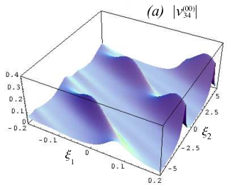
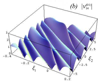
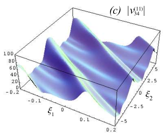
Figure 1: The absolute values of some matrix elements of the particular solution to eq.(2.2) at $\tau_{i}=i$, $i=1,2,3$. Three typical cases are represented. (a) The absolute value of the matrix elements of $v^{(00)}$ and $v^{(10)}$ have the set of upward peaks distributed on the $(\xi_{1},\xi_{2})$-plane, $|v^{(00)}_{34}|$ is shown as an example. (b) The absolute value of the matrix elements of $v^{(01)}$ have upward peaks distributed over the oscillating basis, $|v^{(01)}_{14}|$ is shown as an example. (c) The absolute value of the matrix elements of $v^{(11)}$ have oscillating form without sharp peaks, $|v^{(11)}_{34}|$ is shown as an example.

We see that all matrix elements of $v^{(ij)}$ can be separated into three family. The absolute values of matrix elements from the first family (of the elements of $v^{(00)}$ and $v^{(10)}$, Fig.1a) have high peaks regularly situated on the $(\xi_{1},\xi_{2})$-plane. The absolute values of the matrix elements from the second family (of the elements of $v^{(01)}$, Fig.1b) have peaks situated on the oscillating basis. Finally, the absolute values of the matrix elements from the third family (of the elements of $v^{(11)}$, Fig.1c) have no sharp peaks. So, such $n$-wave type equation can be responsible for forming the lump-type quasi-periodic solutions of large amplitude.

5 Conclusions

We construct a completely integrable linearizable $5$-dimensional version of $n$-wave type equation for the matrix fields $v^{(ij)}$, $i,j=0,1,2$. Its generalization to $2D+1$, $D>2$, case is obvious. We show that the elements of the matrix fields $v^{(ij)}$ have different shapes. Some of them can be viewed as a set of quasi-periodic sharp peaks and thus could be responsible for formation of rogue waves.

It is remarkable, that the auxiliary spectral function $\Psi$ was introduced to derive eq.(3), so that fields $v^{(ij)}$ acquire the spectral representation, similar to the fields of ISTM-integrable nonlinear PDEs. Thus, the dressing method appears here as a tool unifying the nonlinear PDEs integrable by different methods. Similar phenomena have been observed in earlier papers [15, 16], combining nonlinear PDEs integrable by different methods, such as ISTM, linearization by the Hopf substitution, method of characteristics.

Of course, instead of the symmetric form of $\hat{R}_{0}$ (61) we could take its non-symmetric version

$$\hat{R}_{0}(\lambda,\nu)=e^{\sum_{j=1}^{D}s^{(j)}(\lambda)x_{j}+\sum_{k}S^{(k)}(\lambda)t_{k}}R_{0}(\lambda,\mu)e^{\sum_{j=1}^{D}p^{(j)}(\mu)x_{j}+\sum_{k}P^{(k)}(\lambda)t_{k}}.$$ (73)

Then the appropriate nonlinear PDEs would involve the diagonal parts as well.

The work is partially supported by the Program for Support of Leading Scientific Schools (grant No. 9697.2016.2), and by the RFBR (grant No. 14-01-00389).

References

- [1] D. J. Kaup, Stud. Appl. Math. 62, 75 (1980).
- [2] D. J. Kaup, Phys. D 1, 45 (1980).
- [3] C.S.Gardner, J.M.Green, M.D.Kruskal, R.M.Miura, Phys.Rev.Lett, 19, (1967) 1095
- [4] V. E. Zakharov, S. V. Manakov, S. P. Novikov, and L. P. Pitaevsky, Theory of Solitons. The Inverse Problem Method (Plenum Press, 1984).
- [5] M. J. Ablowitz and P. C. Clarkson, Solitons, Nonlinear Evolution Equations and Inverse Scattering (Cambridge University Press, Cambridge, 1991).
- [6] A.B.Shabat, Dokl. Akad. Nauk SSSR 211 No. 6, (1973) 1310
- [7] V.E.Zakharov and A.B.Shabat, Funk.Anal.Pril., 8, (1974) 43; Funct.Anal.Appl., 8, (1974) 226
- [8] V.E.Zakharov and A.B.Shabat, Funct.Anal.Appl. 13, (1979) 13; Funk.Anal.Pril., 13, (1979) 166
- [9] V.E.Zakharov and S.V.Manakov, Funk.Anal.Pril. 19, (1985) 11; Funct.Anal.Appl. 19, (1985) 89
- [10] B. Konopelchenko, Solitons in Multidimensions (World Scientific, Singapore, 1993).
- [11] A.I.Zenchuk, J.Math.Phys. 55, 121505 (2014)
- [12] F. Calogero in What is Integrability ed V.E.Zakharov (Berlin: Springer) (1990) 1
- [13] F. Calogero and Ji Xiaoda, J. Math. Phys. 32, 875 (1991).
- [14] F. Calogero and Ji Xiaoda, J. Math. Phys. 32, 2703 (1991).
- [15] A. I. Zenchuk, J. Phys. A: Math.Gen. 37, 6557 (2004).
- [16] A. I. Zenchuk, J.Math.Phys. 50, 063505 (2009)