Cosmology and Astrophysics Using the Post-reionization HI

Abstract

We discuss the prospects of using the redshifted 21 cm emission from neutral hydrogen in the post-reionization epoch to study our universe. The main aim of the article is to highlight the efforts of Indian scientists in this area with the SKA in mind. It turns out that the intensity mapping surveys from SKA can be instrumental in obtaining tighter constraints on the dark energy models. Cross-correlation of the HI intensity maps with the Ly$\alpha$ forest data can also be useful in measuring the BAO scale.

1 Introduction

The post-reionization ($z\lesssim 6$) evolution of neutral hydrogen (HI) is of great interest from the point of view of both astrophysics as well as cosmology. After reionization, the bulk of HI is expected to reside in galaxies in the form of clumpy, self-shielded clouds (Wolfe et al., 1986; Lanzetta et al., 1991; Storrie-Lombardi & Wolfe, 2000; Gardner et al., 1997; Prochaska et al., 2005). The radio observations of the redshifted 21 cm line promise to be a powerful probe of HI, and it is expected that present and upcoming facilities like the GMRT, MeerKAT, CHIME and SKA would play important roles in this area.

The 21 cm line can used in various ways to study the HI. It is already being used extensively in detecting and studying absorption systems (e.g., DLAs) along lines of sight towards distant radio sources. These studies are complementary to those done using UV / optical telescopes (Prochaska & Wolfe, 2009; Prochaska et al., 2005; Zafar et al., 2013). An alternate way is to detect the HI in emission. The most standard method is to detect individual galaxies in HI through the so called HI galaxy redshift surveys (Barnes et al., 2001; Meyer et al., 2004; Zwaan et al., 2005; Jaffe et al., 2012; Rhee et al., 2013; Giovanelli et al., 2005; Martin et al., 2010; Catinella et al., 2010; Lah et al., 2007, 2009). Another way is to detect only the integrated HI emission of galaxies at each sky location without attempting to resolve the individual objects, a technique known as HI intensity mapping (Bharadwaj & Sethi, 2001; Chang et al., 2010; Masui et al., 2013; Lah et al., 2009). There has been recent surge of investigations aimed towards understanding dark energy using future SKA observations (Guha Sarkar & Datta, 2015; Hussain et al., 2016; Bull et al., 2015b; Zhao et al., 2015; Santos et al., 2015; Bull et al., 2015a).

This article focuses mainly on Indian interests related to studying astrophysics and cosmology using HI emission in the post-reionization universe. The main science cases which have been considered here are (i) the constraints on dark energy using HI intensity mapping experiments, (ii) measuring the BAO using the cross correlation of intensity mapping and Ly$\alpha$ forest.

2 Dark energy constraints from intensity mapping experiments

The large-scale clustering of the HI in the post-reionization epoch is expected to directly probe the nature of dark energy through the imprints of a given model on the background evolution and growth of structures. As a direct probe of cosmological structure formation, 21-cm intensity mapping may allow us to distinguish between dark energy models which are otherwise degenerate at the level of their prediction of background evolution. In the of context of SKA, this has been recently investigated by a group of Indian scientists including the present authors (Hussain et al., 2016).

2.1 Constraints from angular power spectra

To begin with, we consider a very general picture where the two dark components in the universe, dark matter (DM) and dark energy (DE), are interacting with each other. For the dark energy part, we assume the simplest scenario of a canonical scalar field rolling slowly over a very flat potential. The visible sector of the matter consisting baryons is not coupled with DE. This scenario, also known as “Coupled Quintessence" (Amendola, 2000, 2004) is a well studied phenemenological model for dark energy. One can easily switch off the interaction term between DM and DE to consider the case of minimally coupled scalar field dark energy models. The equations governing the spatially flat background universe are as follows (Hussain et al., 2016):

$$\ddot{\phi}+\frac{dV}{d\phi}+3H\dot{\phi}=C(\phi)\rho_{d}$$

$$\dot{\rho}_{d}+3H(\rho_{d})=-C(\phi)\rho_{d}\dot{\phi}$$ (1)

$$\dot{\rho_{b}}+3H(\rho_{b})=0$$

$$H^{2}=\frac{\kappa^{2}}{3}(\rho_{b}+\rho_{d}+\rho_{\phi}).$$

Here $C(\phi)$ represents the coupling between DM and DE. Subscript “d" represents the DM sector and subscript “b" represents the baryonic sector and an overdot represent differential w.r.t comoving time. We still do not know exactly the details physics of interaction bewteen DM and DE; hence our approach is phenomenological where we assume the function $C(\phi)$ to be a constant as in the previous work by Amendola and others (Amendola, 2000, 2004). For $C=0$, we recover the minimally coupled scalar field dark energy model. Hence we can study both the coupled and uncoupled case in the same set up.

We study the growth of matter fluctuations in the linear regime and sub-horizon scales where we can safely igonore the dark energy perturbation. In this regime, Newtonian treament for density perturbation is sufficient for our purpose. With these assumptions, we can write the equations governing the growth of linear fluctuations in dark matter density as:

$$\delta^{\prime\prime}_{d}+\left(1+\frac{\mathcal{H}^{\prime}}{\mathcal{H}}-2Wx\right)\delta^{\prime}_{d}-\frac{3}{2}(\gamma_{d}\delta_{d}\Omega_{d})=0.$$ (3)

Here prime denotes differentiation w.r.t to $\log a$ and $x=\frac{\kappa\dot{\phi}}{\sqrt{6}H}$. Here $W=\frac{C}{\kappa}$, $\gamma_{d}=1+2W^{2}$, ${\mathcal{H}}$ is the conformal Hubble parameter ${\mathcal{H}=aH}$ and $\delta_{d}$ is the linear density contrast for the DM. We solve the equation with the initial conditions at decoupling ($a\sim 10^{-3}$) when $\delta_{d}\sim a$ and $\frac{d\delta_{d}}{da}=1$.

Taking the Fourier transform of the above equation, we define the linear growth function $D_{d}$ and the linear growth rate $f_{d}$ as

$$\delta_{dk}(a) \equiv D_{d}(a)\delta_{dk}^{ini}$$ (4)

$$f_{d} = \frac{d\ln{D_{d}}}{d\ln{a}}.$$ (5)

The linear dark matter power spectrum given by

$$P(k,z)=A_{0}k^{n_{s}}T^{2}(k)D_{dn}^{2}(z).$$ (6)

Here $A_{0}$ is the normalization constant and we fix it using $\sigma_{8}$ value at present from Planck 2015 observations (Ade et al., 2016), $n_{s}$ is spectral index for the primordial density fluctuations generated through inflation, $D_{dn}(z)$ is growth function normalized such as it is equal to unity at $z=0$ i.e. $D_{dn}(z)=\frac{D_{d}(z)}{D_{d}(0)}$. $T(k)$ is the transfer function as given by Eisenstein and Hu (Eisenstein & Hu, 1999).

To constrain dark energy behaviour using the 21-cm intensity mapping, the quantity of interest is the fluctuations in the HI 21-cm brightness temperature $\delta T_{b}$ and its corresponding angular power spectra which in the flat sky limit is given by (Datta et al., 2007)

$$C_{l}=\frac{{\bar{T}}^{2}\bar{x}_{HI}^{2}b_{T}^{2}}{\pi r^{2}}\int\limits_{0}^{\infty}dk_{\parallel}~{}(1+\beta_{T}\mu^{2})^{2}~{}P(k,z).$$ (7)

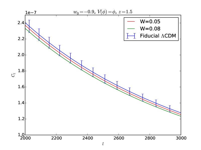
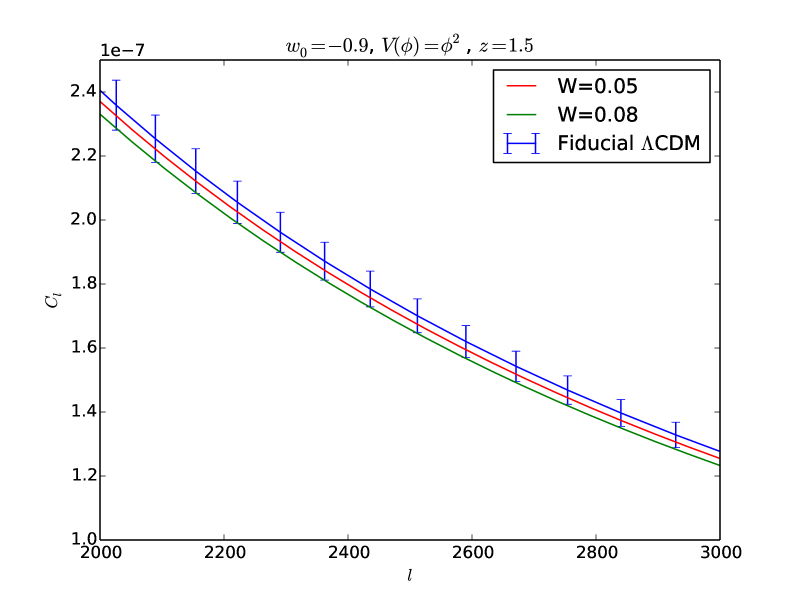
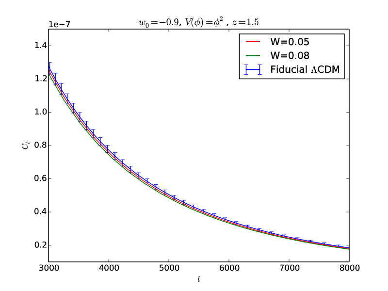
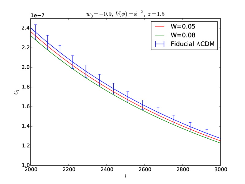
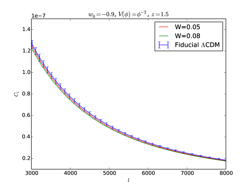
Figure 1: Angular power spectra for the fluctuations in HI 21-cm brightness tempertaure for different dark scalar field with different potentials $V(\phi)$ and coupling parameter $W$. The left colomn is for $2000\leq l\leq 3000$ and the right colomn is for $3000\leq l\leq 8000$.

Here $P(k,z)$ is the dark matter power spectrum defined in equation (6). $k=\sqrt{k_{\parallel}^{2}+\frac{l^{2}}{r^{2}}}$, $r$ being the comoving distance at a certain redshift $z$, $\mu=\frac{k_{\parallel}}{k}$ and $\beta_{T}=\frac{f_{d}(z)}{b_{T}}$ where $f_{d}(z)$ is the growth factor for dark matter defined in equation (5). $b_{T}$ is the linear bias parameter. The average brightness temperature $\bar{T}$ at redshift $z$ is given by

$$\bar{T}(z)=4.0{\rm mK}(1+z)^{2}\left(\frac{\Omega_{b0}h^{2}}{0.02}\right)\left(\frac{0.7}{h}\right)\left(\frac{H_{0}}{H(z)}\right).$$ (8)

We assume $\Omega_{HI}=10^{-3}$ for $z<3.5$. This gives $\bar{x}_{HI}=2.45\times 10^{-2}$ and we assumed this to be constant across the redshift range of our interest. Also our assumption of flat sky approximation is valid for $l>200$ (Datta et al., 2007).

We consider a radio interferometric measurement of the power spectrum of the HI 21-cm brightness temperature. The noise in our measurement of angular power spectrum comes from instrumental noises on smalls scales and cosmic variances on large scales. This is given by

$${\Delta C_{l}}=\sqrt{\frac{2}{(2l+1)\Delta lf_{sky}N_{p}}}\left(C_{l}+N_{l}\right).$$ (9)

where $N_{p}$ being the number of pointings of the radio interferometer, $f_{sky}$ is the fraction of sky observed in a single pointing, and $\Delta l$ is the width of the $l$ bin and $N_{l}$ is the noise power spectrum.

To calculate $\Delta C_{l}$, we use the following specifications of SKA1-mid :

We consider the fiducial redshift $z=1.5$ which corresponds to an observing frequency of $568{\rm MHz}$ that falls in the band of frequencies to be probed by SKA1-mid. The frequency bandwidth is $32{\rm MHz}$ around the central frequency. The array consists of 200 dishes each of diameter $15$m. The antennae are distributed in a manner such that $75\%$ of the dishes are within $2.5$Km radius and the number density of antennae are assumed to fall off radially as $r^{-2}$. We note that $T_{sky}=180\left(\frac{\nu}{180{\rm MHz}}\right)^{-2.6}$ K. in our error estimates. However, the total system temperature $T_{syst}$ has a contribution from both the sky temperature and instrumental noise. In this paper we have used $T_{syst}=40$K from the SKA document . Our fiducial model for error calculations is a $\Lambda$CDM model with $\Omega_{\Lambda}=0.7$, $\Omega_{b0}=0.05$, $n_{s}=1$, $h=0.7$ and $\sigma_{8}=0.8$. We also fix the value of the constant linear bias at the value $1.0$. For detail derivation of the noise, we refer readers to (Hussain et al., 2016). The noise is estimated by considering a radio observation of 10,000 hrs distributed equally over 40 pointings. It has been noted that in intensity mapping experiments it is imperative to cover large observational volumes rather than have a deep probe of a small part of the sky.

The results of our analysis is shown in figures 1 and 2. In figure 1, we show the angular power spectra $C_{l}$ for the fluctuations in the HI 21-cm brightness temperature for scalar field model with different potentials and for different values for the coupling parameter $W$. We normalize all the models to have the same present day value of the equation of state, $w_{0}=-0.9$ and density paremeter for the dark energy $\Omega_{\phi 0}=0.7$. In each plot, we also show the $C_{l}$ for our fidcucial $\Lambda$CDM model and the corresponding error bars for SKA1-mid. The figures show that for higher values of the coupling parameter $W$, it may be possible to distinguish scalar field models from $\Lambda$CDM by SKA1-mid for smaller angular scales (higher $l$’s). We concentrate scales in the range of $l\geq 2000$ where we neglect the relativistic corrections as well as corrections due to DE perturbations.

Next to see what happens when we turn off the coupling between the DM and DE, in figure 2 (left), we show the same plot as in figure 1 but only for linear potential with $W=0.8$ and $W=0$ which clearly shows that it may not be possible to distinguish minimally coupled ($W=0$) scalar field from $\Lambda$CDM model by SKA1-mid. Although we show it for linear potential, but the result holds for other potentials as well.

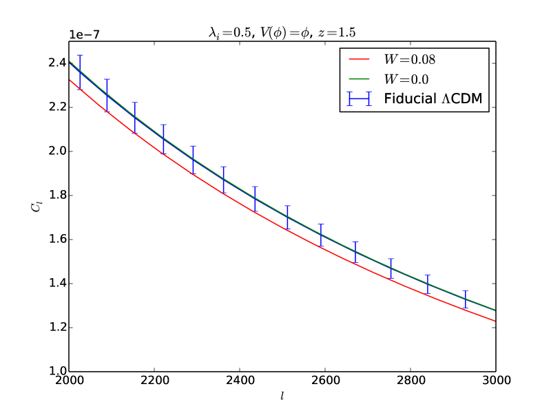
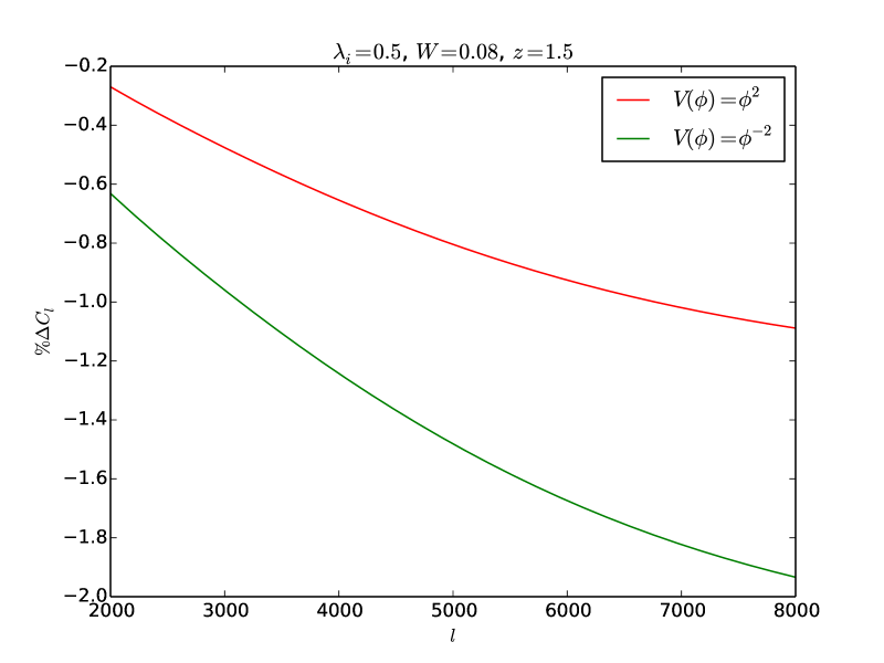
Figure 2: Left: Angular power spectra for the fluctuations in HI 21-cm brightness tempertaure for different dark scalar field wih linear potential for coupled and uncoupled case. Right: Percentage deviation in $C_{l}$ for square and inverse-square potentials from the linear potential in coupled case. Here $\lambda_{i}=-\frac{1}{V(\phi)}\frac{dV(\phi)}{d\phi}|_{z=1000}$

Finally to see whether we can distinguish between different potentials for coupled scalar field models, in figure 2 (right), we show the percentage deviation in $C_{l}$ for square and inverse square potentials from the linear potentials. It shows that inverse-square potential has a greater deviation from linear potential and hence is more probable to be distinguished from the linear potential.

3 Constraints from BAO measurements using different diagnostics

Primordial cosmological density fluctuations drive acoustic waves in the cosmological baryon-photon plasma which gets frozen once recombination takes place at about $z\sim 1000$. This leaves a distinct oscillatory signature on the CMBR temperature anisotropy power spectrum (Peebles & Yu, 1970). The sound horizon at the epoch of recombination sets a standard ruler that maybe used to calibrate cosmological distances. Baryons contribute to $15\%$ of the total matter budget, and the baryon acoustic oscillations (BAO) are hence also imprinted in the late time clustering of non-relativistic matter. The baryon acoustic oscillation (BAO) is a powerful probe of cosmological parameters (Seo & Eisenstein, 2003). Measuring BAO signal allows us to measure the angular diameter distance $D_{A}$ and the Hubble parameter $H(z)$ as functions of redshift using the the transverse and the longitudinal oscillations respectively. These provide means for placing strong constraints on dark energy models. The cross-correlation of the Ly-$\alpha$ forest and redshifted 21-cm emission from the post-reionization epoch is believed to be a tool for mapping out the large-scale structures for redshifts $z\leq 6$. This mitigates several observational issues like foreground subtraction which poses serious challenge towards detecting the 21-cm signal. The possibility of detecting the BAO signal with the cross-correlation signal is investigated in (Sarkar & Bharadwaj, 2013).

For the Ly-$\alpha$ forest survey, we have considered typical surveys like BOSS and BIGBOSS which are expected have a high number density of quasars of $16\ {\rm deg}^{-2}$ and $64\ {\rm deg}^{-2}$ respectively. We are interested in measuring $\delta q_{1}=\delta H(z)/H(z)$, $\delta q_{2}=\delta D_{A}/D_{A}$ and also $\delta D_{V}/D_{V}$ where $D_{V}^{3}=(1+z)^{2}D_{A}(z)cz/H(z)$ is a combined distance measure using the cross-correlation power spectrum $P_{FT}$ between the Lyman-slpha transmitted flux and the 21-cm brightness temperature. We estimate the errors using a Fisher matrix analysis. The cross-power spectrum is given by

$$P_{FT}({\bf k})=\bar{T}(z){\bar{x}}_{\rm HI}b_{T}C_{F}(1+\beta_{F}\mu^{2})(1+\beta_{T}\mu^{2})P(k)$$ (10)

We have adopted $(C_{F},\beta_{F})=(=0.15,1.11)$ from numerical simulation of the Lyman-alpha forest (McDonald, 2003).

The $2\times 2$ Fisher matrix for estimation of parameters is given by

$$F_{ij}=\frac{\cal V}{2\pi^{3}}\int\frac{d^{3}{\bf k}}{\left[P_{FT}^{2}+(P_{F}+N_{F})(P_{T}+N_{T})\right]}\frac{\partial P_{FT}}{\partial q_{i}}\frac{\partial P_{FT}}{\partial q_{j}}$$ (11)

where $\cal V$ is the survey volume and $P_{F}$ and $P_{T}$ denote the auto power spectrum of Lyman alpha forest and 21 cm signal respectively, and $N_{F}$ and $N_{T}$ denote the corresponding noise power spectra. We have $N_{F}=\frac{1}{\bar{n}_{Q}}(P_{F}^{1D}+\sigma^{2})$, where $\bar{n}_{Q}$ is the quasar density in the field. The aliasing term $P_{F}^{1D}$ is obtained by integrating the 3D power spectrum and the pixel noise contribution $\sigma^{2}$ is obtained by assuming that the spectra are measured at an average $3-\sigma$ level. The details of the analysis maybe found in Guha Sarkar & Datta (2015). The Cramer-Rao bound on the error are given by $\delta q_{i}=\sqrt{F^{-1}_{ii}}$ and $\delta D_{V}/D_{V}=\frac{1}{3}(4F^{-1}_{11}+4F^{-1}_{12}+F^{-1}_{22})^{0.5}$. The noise power spectrum for the 21 cm signal is given by

$$N_{T}=1.0\times 10^{-3}mK^{2}\left(\frac{500}{N_{ant}}\right)^{2}\left(\frac{100\rm KHz}{\Delta\nu}\right)\left(\frac{1000hrs}{t_{obs}}\right).$$ (12)

where $N_{ant}$, $\Delta\nu$ and $t_{obs}$ denote number of antennae, bandwidth and observation time per pointing. Here we have assumed that two polarizations have been used. We have used a $32$MHz bandwidth observation and the same number of antennae as before. For simplicity, here we have assumed antenna distribution to be such that it gives an uniform distribution of baselines. We find that it is necessary to achieve a noise level of $N_{T}=1.1\times 10^{-5}\ {\rm mK}^{2}$ and $N_{T}=6.25\times 10^{-6}\ {\rm mK}^{2}$ per field of view in the redshifted 21-cm observations to detect the angular and radial BAO respectively with BOSS at a redshift $z=2.5$. The corresponding noise levels are $3.3\times 10^{-5}\ {\rm mK}^{2}$ and $1.7\times 10^{-5}\ {\rm mK}^{2}$ for BIGBOSS. These noise levels should be attainable by $10000$ hrs observations distributed equally over 100 pointings with SKA1-mid roughly covering the full sky coverage of BOSS. It is possible to measure the distance measure $D_{V}$ with $D_{V}^{3}=(1+z)^{2}D_{A}(z)cz/H(z)$ at $\delta D_{V}/D_{V}=2\%$ from the cross-correlation signal with $N_{T}=3\times 10^{-4}$ mK². We have $(\delta D_{V}/D_{V},\delta D_{A}/D_{A},\delta H/H)=(1.3,1.5,1.3)\%$ and $(0.67,0.78,0.74)\%$ at $N_{T}=10^{-4}{\rm mK}^{2}$ and $N_{T}=10^{-5}{\rm mK}^{2}$ at the fiducial redshift $z=2.5$. The quasar pixel noise is held constant to a $3-\sigma$ in units of the mean transmitted flux. The results are shown in figure 3.

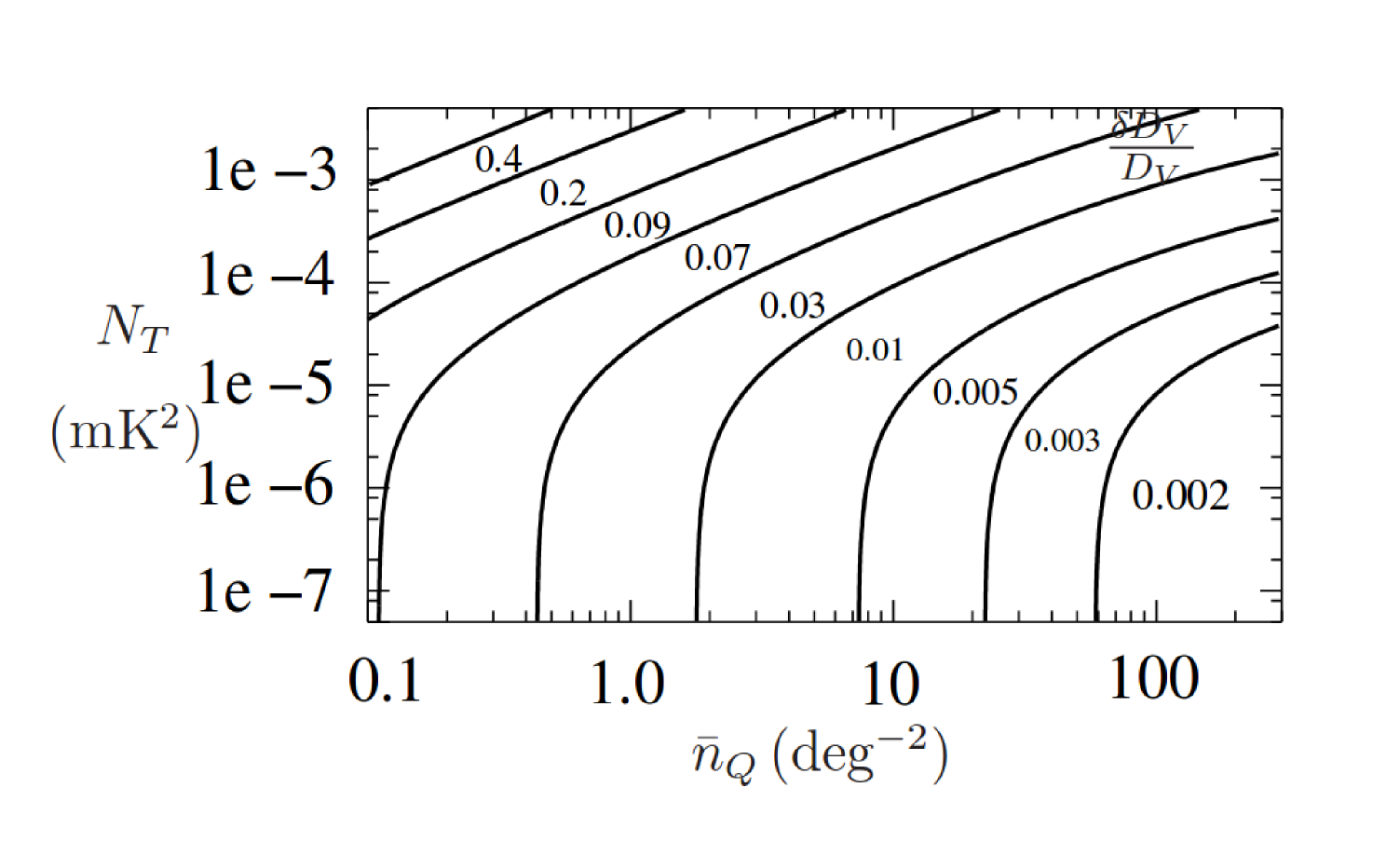
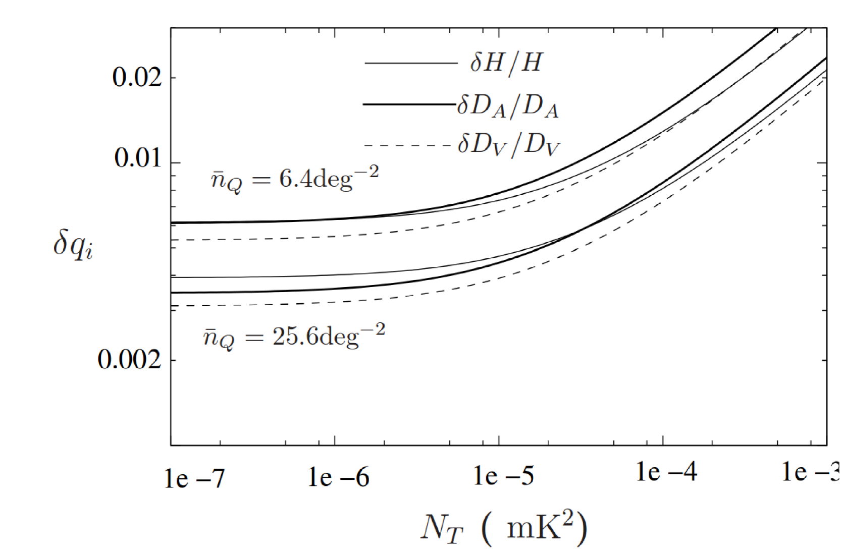
Figure 3: Left: The error contours for the distance measure $D_{V}$ Right: Error prediction for BOSS and BIGBOSS. Figures from (Sarkar & Bharadwaj, 2013). We find that at large $N_{T}$ there is a rough scaling $\delta q_{i}\propto N_{T}^{0.5}$.

4 Summary

The 21 cm line from HI in the post-reionization universe can be a strong probe of cosmology and galaxy formation. We discuss the efforts of the Indian scientists in this area in the context of future SKA survey. We discuss the predictions and forecasts for probing a large class of scalar field dark energy models using angular power spectra for the intensity mapping from SKA. Although we restrict ourselves to canonical scalar field models, but the study can be easily extended to more general class of non-canonical and Hordenski class of models for scalar field. We also show that the intensity mapping experiments can be useful in probing the BAO, in particular, when the data is cross correlated with Ly$\alpha$ forest experiments like the BIGBOSS. And this in turn can be used to constrain dark energy models.

The main obstacle in detecting the cosmological redshifted 21-cm signal is the presence of foregrounds from astrophysical galactic and extra galactic sources. These are several orders of magnitude larger than the actual signal. We should therefore carefully subtract these foregrounds before an accurate statistical detection of the cosmological signal is confirmed. In this regard, the cross-correlation studies discussed here are expected to be more efficient in dealing with the experimental systematics. With a number of facilities (SKA, Euclid, LSST) expected to be active in different wave bands in coming years, the future thus looks promising.

References

- Ade et al. (2016) Ade P. A. R., et al., 2016, Astron. Astrophys., 594, A13
- Amendola (2000) Amendola L., 2000, Phys. Rev. D , 62, 043511
- Amendola (2004) Amendola L., 2004, Phys. Rev. D , 69, 103524
- Barnes et al. (2001) Barnes D. G., et al., 2001, Mon. Not. Roy. Ast. Soc. , 322, 486
- Bharadwaj & Sethi (2001) Bharadwaj S., Sethi S. K., 2001, Journal of Astrophysics and Astronomy, 22, 293
- Bull et al. (2015a) Bull P., Camera S., Raccanelli A., Blake C., Ferreira P., Santos M., Schwarz D. J., 2015a, Advancing Astrophysics with the Square Kilometre Array (AASKA14), p. 24
- Bull et al. (2015b) Bull P., Ferreira P. G., Patel P., Santos M. G., 2015b, Astrophys. J., 803, 21
- Catinella et al. (2010) Catinella B., et al., 2010, Mon. Not. Roy. Ast. Soc. , 403, 683
- Chang et al. (2010) Chang T.-C., Pen U.-L., Bandura K., Peterson J. B., 2010, Nature , 466, 463
- Datta et al. (2007) Datta K. K., Choudhury T. R., Bharadwaj S., 2007, Mon. Not. Roy. Ast. Soc. , 378, 119
- Eisenstein & Hu (1999) Eisenstein D. J., Hu W., 1999, Astroph. J. , 511, 5
- Gardner et al. (1997) Gardner J. P., Katz N., Hernquist L., Weinberg D. H., 1997, Astroph. J. , 484, 31
- Giovanelli et al. (2005) Giovanelli R., et al., 2005, Astron. J. , 130, 2598
- Guha Sarkar & Datta (2015) Guha Sarkar T., Datta K. K., 2015, J. Cosmology Astropart. Phys., 8, 001
- Hussain et al. (2016) Hussain A., Thakur S., Guha Sarkar T., Sen A. A., 2016, preprint, (arXiv:1603.02087, to appear in MNRAS)
- Jaffe et al. (2012) Jaffe Y. L., Poggianti B. M., Verheijen M. A. W., Deshev B. Z., van Gorkom J. H., 2012, Astrophys. J., 756, L28
- Lah et al. (2007) Lah P., et al., 2007, Mon. Not. Roy. Ast. Soc. , 376, 1357
- Lah et al. (2009) Lah P., et al., 2009, Mon. Not. Roy. Ast. Soc. , 399, 1447
- Lanzetta et al. (1991) Lanzetta K. M., Wolfe A. M., Turnshek D. A., Lu L., McMahon R. G., Hazard C., 1991, ApJS, 77, 1
- Martin et al. (2010) Martin A. M., Papastergis E., Giovanelli R., Haynes M. P., Springob C. M., Stierwalt S., 2010, Astroph. J. , 723, 1359
- Masui et al. (2013) Masui K. W., et al., 2013, ApJ, 763, L20
- McDonald (2003) McDonald P., 2003, Astroph. J. , 585, 34
- Meyer et al. (2004) Meyer M. J., et al., 2004, Mon. Not. Roy. Ast. Soc. , 350, 1195
- Peebles & Yu (1970) Peebles P. J. E., Yu J. T., 1970, Astroph. J. , 162, 815
- Prochaska & Wolfe (2009) Prochaska J. X., Wolfe A. M., 2009, Astroph. J. , 696, 1543
- Prochaska et al. (2005) Prochaska J. X., Herbert-Fort S., Wolfe A. M., 2005, Astroph. J. , 635, 123
- Rhee et al. (2013) Rhee J., Zwaan M. A., Briggs F. H., Chengalur J. N., Lah P., Oosterloo T., van der Hulst T., 2013, Mon. Not. Roy. Ast. Soc. , 435, 2693
- Santos et al. (2015) Santos M., et al., 2015, Advancing Astrophysics with the Square Kilometre Array (AASKA14), p. 19
- Sarkar & Bharadwaj (2013) Sarkar T. G., Bharadwaj S., 2013, JCAP, 1308, 023
- Seo & Eisenstein (2003) Seo H., Eisenstein D. J., 2003, Astroph. J. , 598, 720
- Storrie-Lombardi & Wolfe (2000) Storrie-Lombardi L. J., Wolfe A. M., 2000, Astroph. J. , 543, 552
- Wolfe et al. (1986) Wolfe A. M., Turnshek D. A., Smith H. E., Cohen R. D., 1986, ApJS, 61, 249
- Zafar et al. (2013) Zafar T., Péroux C., Popping A., Milliard B., Deharveng J.-M., Frank S., 2013, A&A, 556, A141
- Zhao et al. (2015) Zhao G., Bacon D., Maartens R., Santos M., Raccanelli A., 2015, Advancing Astrophysics with the Square Kilometre Array (AASKA14), p. 165
- Zwaan et al. (2005) Zwaan M. A., Meyer M. J., Staveley-Smith L., Webster R. L., 2005, Mon. Not. Roy. Ast. Soc. , 359, L30