Probing individual sources during reionization and cosmic dawn using SKA HI 21-cm observations

Abstract

Detection of individual luminous sources during the reionization epoch and cosmic dawn through their signatures in the HI 21-cm signal is one of the direct approaches to probe the epoch. Here, we summarize our previous works on this and present preliminary results on the prospects of detecting such sources using the SKA1-low experiment. We first discuss the expected HI 21-cm signal around luminous sources at different stages of reionization and cosmic dawn. We then introduce two visibility based estimators for detecting such signal: one based on the matched filtering technique and the other relies on simply combing the visibility signal from different baselines and frequency channels.

We find that that the SKA1-low should be able to detect ionized bubbles of radius $R_{b}\gtrsim 10$ Mpc with $\sim 100$ hr of observations at redshift $z\sim 8$ provided that the mean outside neutral Hydrogen fraction $x_{{\rm H~{}{\sc I}\,}}\gtrsim 0.5$. We also investigate the possibility of detecting HII regions around known bright QSOs such as around ULASJ1120+0641 discovered by Mortlock et al. (2011). We find that a $5\sigma$ detection is possible with $600$ hr of SKA1-low observations if the QSO age and the outside $x_{{\rm H~{}{\sc I}\,}}$ are at least $\sim 2\times 10^{7}$ Myr and $\sim 0.2$ respectively.

Finally, we investigate the possibility of detecting the very first X-ray and Ly-$\alpha$ sources during the cosmic dawn. We consider mini-QSOs like sources which emits in X-ray frequency band. We find that with a total $\sim 1000$ hr of observations, SKA1-low should be able to detect those sources individually with a $\sim 9\sigma$ significance at redshift $z=15$. We summarize how the SNR changes with various parameters related to the source properties.

1 Introduction

The emergence of first galaxies, quasars in the Universe is one of the significant events in its history. In the standard scenario, the Ly-$\alpha$, X-ray, UV photons produced by these first sources percolated through the intergalactic medium (IGM) and completely altered its thermal and ionization state. Unfortunately, we know very little about this landmark event and nature and properties of first sources .

Recently, tens of extremely bright quasars at redshifts $z\gtrsim 6$ have been detected by various surveys (Fan et al., 2006; Mortlock et al., 2011; Venamans et al., 2015). In addition, hundreds of high redshift galaxies at similar redshifts have been discovered by various telescopes (Ouchi et al., 2010; Hu et al., 2010; Kashikawa et al., 2011; Ellis et al., 2013; Bouwens et al., 2015). These sources are expected to have played an important role during the reionization epoch. We expect many such sources to exist even at higher redshifts during the initial stage of reionization and cosmic dawn.

It is likely that the UV photons from these sources ionized the neutral Hydrogen (H I) atoms around them and created H II regions (ionized bubbles) which are embedded in H I medium. The Ly-$\alpha$ from the very first luminous sources during the cosmic dawn coupled the IGM temperature with HI spin temperature. Similarly the X-ray photons from X-ray sources heated up the IGM and therefore raised both the IGM kinetic and the HI spin temperature. The coupling and the heating are initially efficient near the sources. Previous studies showed that it is possible to detect the 21-cm signatures around these individual sources using current low-frequency telescopes (Datta, Bharadwaj & Choudhury, 2007; Geil & Wyithe, 2008; Datta et al., 2008; Datta, Bharadwaj & Choudhury, 2009; Malloy & Lidz, 2013) which would be useful in constraining the IGM and source properties (Majumdar, Bharadwaj & Choudhury, 2012; Datta et al., 2012). We also expect that upcoming space telescopes such as the James Webb Space Telescope (JWST) should also be able to detect some of these brightest sources during the cosmic dawn and reionization epoch in the optical/infrared band (Zackrisson et al., 2011; De Souza et al., 2013, 2014).

One of the straightforward approaches to understand the reionization epoch and cosmic dawn is to detect individual luminous sources through their signature on the HI 21-cm signal. Existing low frequency radio telescopes such as the GMRT, MWA, LOFAR primarily aim to detect the HI 21-cm signal statistically by measuring quantities such as the power spectrum, rms, skewness of the HI 21-cm brightness temperature fluctuations. Here, we take an alternative but direct approach to explore the reionization epoch and cosmic dawn through detection of HI 21-cm signature around individual sources. In this paper, our aim is to summarise our previous works on this issue and present some preliminary results on the prospects of detecting such sources using the SKA1-low experiment which is the low frequency part of the Square Kilometer Telescope to be built in phase 1. With much higher number antenna, better baseline coverage and detectors, the SKA1-low is expected to be much more sensitive telescope for detecting such objects individually with much less observation time (Ghara et al., 2016; Mellema et al., 2013, 2015). After a brief discussion on nature of the expected HI 21-cm signal around luminous sources at different stages of reionization and cosmic dawn, we introduce two visibility based methods for detecting such signal: (i) the first method is based on the matched filtering principle which was first introduced in Datta, Bharadwaj & Choudhury (2007) and explored in detail in subsequent works (Datta et al. (2008); Datta, Bharadwaj & Choudhury (2009); Datta et al. (2012), Majumdar et al. (2011); Majumdar, Bharadwaj & Choudhury (2012), Malloy & Lidz (2013) ) and (ii) the second method relies on simply combing the visibility signal from different baselines and frequency channels (Ghara, Choudhury & Datta (2016)).

The outline of the article is as follows: In section 2, we discuss the HI 21-cm signal profile around individual sources during the cosmic dawn and reionization epoch. In subsection 2.3, we calculate and discuss corresponding visibility signal. Section 3 discusses two visibility based estimators which have been developed for detecting the signal discussed in section 2. We also describe the filter we consider for the first estimator which uses the matched filter technique. Section 4 discusses the results on the detectability of ionized bubbles, known bright QSOs in the reionization epoch and the first sources during the cosmic dawn using SKA1-low telescope. Section 5 presents a summary of the paper.

2 The HI 21-cm signal around individual sources

The first sources are expected to emit in UV, Ly-$\alpha$, X-ray frequencies. In a likely scenario, a fraction of the Ly-$\alpha$ photons from the first generation of stars escape from their host environment and couple the H I spin temperature with the IGM gas kinetic temperature very quickly. At the same time the soft X-ray photons emitting from sources like the mini-QSOs, X-ray binaries, Pop III stars etc. enter into the IGM and heat it up. This causes the HI spin temperature above the background CMB temperature. Subsequently, the UV photons start ionizing HI surrounding the sources and create ionized bubbles which are embedded into HI medium. The Ly-$\alpha$ coupling, X-ray heating, and UV ionization are initially done near the sources and slowly spread over the entire IGM. We expect three distinct differential HI 21-cm brightness temperature ($\delta T_{b}$) profiles around sources at three different stages of the cosmic dawn and reionization. In general, the differential brightness temperature of the HI 21-cm signal can be written as

$$\delta T_{b}(\vec{\theta},\nu)\!\!\!\! = \!\!\!\!27~{}x_{\rm HI}(\mathbf{x},z)[1+\delta_{\rm B}(\mathbf{x},z)]\left(\frac{\Omega_{B}h^{2}}{0.023}\right)$$

$$\times \!\!\!\!\left(\frac{0.15}{\Omega_{m}h^{2}}\frac{1+z}{10}\right)^{1/2}\left[1-\frac{T_{\rm CMB}(z)}{T_{\rm S}(\mathbf{x},z)}\right]\,\rm{mK},$$

where $\mathbf{x}=r_{z}\mathbf{\hat{n}}$ and $1+z=1420~{}{\rm MHz}/\nu_{\rm obs}$, $r_{z}$ is the radial comoving distance to redshift $z$. $\delta_{\rm B}(z,\mathbf{x})$ and $x_{\rm HI}(z,\mathbf{x})$ denote the density contrast in baryons and HI fraction respectively at $\mathbf{x}$ at a redshift $z$. $T_{\rm CMB}(z)$ = 2.73 $\times(1+z)$ K is the CMB temperature at a redshift $z$ and $T_{\rm S}$ is the spin temperature of H I gas. We ignore the line of sight peculiar velocity effects (Bharadwaj & Ali, 2004; Barkana & Loeb, 2005) in the above expression, which, we believe do not affect the results presented here.

Below, we briefly discuss the HI 21-cm brightness temperature profile around individual sources expected at different stages of reionization and cosmic dawn.

2.1 Model A: HI 21-cm signal from ionized bubbles during reionization

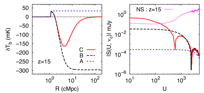
Figure 1: Left panel: The differential brightness temperature profile around an isolated mini-QSO. The source properties are taken to be those corresponding to the fiducial values. The results are shown for all three coupling models A, B, C described in the texts. Right panel: The absolute value of the corresponding visibility amplitude as a function of baseline U. Also shown are rms noise in the visibilities calculated for $1000$ h of observation with the SKA1-low with a frequency resolution of $50\,{\rm kHz}$. The minimum baseline $U_{\rm min}=10$ for the observation we consider here. The figure is taken from our previous work Ghara, Choudhury & Datta (2016).

In this scenario, we assume that the IGM kinetic temperature is fully coupled with the HI spin temperature and both the temperatures are much higher than the CMB temperature. This is a likely scenario when there are sufficient X-ray, Ly-$\alpha$ sources during the cosmic dawn and the Universe is already $\sim 10-20\%$ ionized or after that. Now, we consider a spherical ionized bubble of comoving radius $R_{b}$ centered at redshift $z_{c}$ surrounded by uniform IGM with H I fraction $x_{\rm HI}$. We refer this as model A. These kind of ionized bubbles are expected to be common during the later stages of reionization as there are a significant numbers of UV sources which create spherical ionized regions around them. We note that this model was introduced and the formalism for calculating the visibility signal was developed first in Datta, Bharadwaj & Choudhury (2007). Here and in the subsection 2.3, we discuss the key equations for calculating the visibility signal.

A bubble of comoving radius $R_{b}$ will be seen as a circular disc in each of the frequency channels that cut through the bubble. At a frequency channel $\nu$, the angular radius of the disc is $\theta_{\nu}=(R_{b}/r_{\nu})\sqrt{1-(\Delta\nu/\Delta\nu_{b})^{2}}$, where $\Delta\nu=\nu-\nu_{c}$ is the distance from the bubble’s centre $\nu_{c}=1420\,{\rm MHz}/(1+z_{c})$ and $\Delta\nu_{b}=R_{b}/r^{\prime}_{\nu}$, $\Delta\nu_{b}$ is the bubble’s radius in frequency space. Here, $r_{\nu}$ is the comoving distance corresponding to $z=(1420\,{\rm MHz}/\nu)-1$ and $r^{\prime}_{\nu}=dr_{\nu}/d\nu$. The specific intensity profile of HI 21-cm signal in this scenario can be written as

$$I_{\nu}(\vec{\theta})=\bar{I}_{\nu}x_{\rm HI}\left[1-\Theta\left(1-\frac{\mid\vec{\theta}-\vec{\theta}_{c}\mid}{\theta_{\nu}}\right)\right]\Theta\left(1-\frac{\mid\nu-\nu_{c}\mid}{\Delta\nu_{b}}\right)$$ (2)

where the radiation from the uniform background HI distribution with H I fraction $x_{\rm HI}$ can be written as $x_{\rm HI}$ $\bar{I_{\nu}}$ where $\bar{I_{\nu}}=2.5\times 10^{2}\frac{Jy}{sr}\left(\frac{\Omega_{b}h^{2}}{0.02}\right)\left(\frac{0.7}{h}\right)\left(\frac{H_{0}}{H(z)}\right)$ and $\Theta(x)$ is the Heaviside step function. Note that, here we assume $T_{S}>>T_{\rm CMB}$, H I overdensity parameter $\delta_{B}=0$. In the Raleigh-Jeans limit the specific intensity $\bar{I}_{\nu}$ in eq. 2 can be calculated from the differential brightness temperature in eq. LABEL:eq:brightnessT using the relation $\bar{I}_{\nu}=\left(\frac{2K_{B}}{\lambda^{2}}\right)\delta T_{b}(\vec{\theta},\nu)$.

The dashed blue line in the left panel of figure 1 shows the HI differential brightness temperature profile as a function of comoving distance from the source. As mentioned above, we assume $T_{\rm S}>>T_{\rm CMB}$ here. The differential brightness temperature is zero very close to the source because the region is highly ionised and equals to the background HI differential brightness temperature far from the source.

2.2 Model B & C: 21-cm signal around sources during cosmic dawn

In model B, the Ly-$\alpha$ coupling is assumed to be efficient throughout i.e, the IGM kinetic temperature is completely coupled with the HI spin temperature. Additionally, we assume that there is a X-ray source at the centre of a host DM halo. We refer this as model B. In this model the HI 21-cm signal pattern, in general, can be divided into three prominent regions: (i) the signal is absent inside the central ionized (H II) bubble of the source. (ii) The H II (ionized) region is followed by a region which is neutral and heated by X-rays. In this region, the IGM kinetic temperature $T_{K}>T_{\rm CMB}$ and thus the HI 21-cm signal is seen in emission. (iii) The third is a strong absorption region which is colder than $T_{\rm CMB}$ as the X-rays photons have not been able to penetrate into this region. At reasonably far from the source the spin temperature eventually becomes equal to the background IGM temperature.

We consider a third model, referred as model C, which calculates the Ly-$\alpha$ coupling, heating, ionisation self-consistently. This is believed to be the case at very early stages of the cosmic dawn. In addition to all three prominent regions described in the model B there will one more prominent region i.e, Beyond the absorption region, the signal gradually approaches to zero as the Ly -$\alpha$ coupling becomes less efficient at the region far away from the source.

Here, we consider only mini-QSOs as a X-ray sources (see Ghara, Choudhury & Datta (2016) for other X-rays sources). The stellar mass for this source model is taken to be $M_{\star}=10^{7}\,M_{\odot}$. The value of the escape fraction is taken to be $f_{\rm esc}=0.1$. The X-ray to UV luminosity is fixed as $f_{X}=0.05$, while the power law index of the X-ray spectrum of mini-QSO model is chosen to be $\alpha=1.5$. It is assumed that the age of the sources is $t_{\rm age}=20$ Myr. The densities of hydrogen and helium in the IGM are assumed to be uniform and the density contrast $\delta$ is set to $0$. We denote this model source as our “fiducial” model. We choose the fiducial redshift to be $15$ for presenting our results.

The black dashed and the solid red lines in the left panel of the figure 1 show the 21-cm differential brightness temperature $\delta T_{b}$ profile around a mini-QSO like source described above for the B and C models respectively.

2.3 Visibilities

The expected visibility signal in each frequency channel is the Fourier transform of the sky intensity pattern and can be approximated as (see Datta, Bharadwaj & Choudhury (2007) for the model A, and the Appendix A of Ghara, Choudhury & Datta (2016) for the B and C models)

$$S^{(i)}(U,\nu)\approx-2mx_{\rm HI}\pi I_{\nu,i}\theta^{2}_{\nu,i}\left[\frac{J_{1}(2\pi U\theta_{\nu,i})}{2\pi U\theta_{\nu,i}}\right]\Theta\left(1-\frac{|\nu-\nu_{c}|}{\Delta\nu_{b,i}}\right).$$ (3)

We assume that the source is at the phase centre of the antenna field of view. $i$ denotes various models such as model A, B, C. The integer $m=1$ for the A and C model and $-1$ for the B model. The above visibility signal picks up an extra phase factor if the source is not at the centre of the field of view. The right panel of Fig: 1 shows the visibility signal $S^{(i)}(U,\nu)$ as a function of baseline $U$ for the central frequency channel.

For the model A, the HI 21-cm signal is zero within a circular disc through an ionized bubble of radius $R_{\rm b,A}$. In each channel of frequency $\nu$, the signal has a peak value $|S(0,\nu)|=\pi x_{\rm HI}\bar{I}_{\nu,A}\theta^{2}_{\nu,A}$. The signal is largely contained within baselines $U\leq U_{0}=0.61/\theta_{\nu,A}$ (blue dashed line in the right panel of figure 1), where the Bessel function has its first zero crossing, and the signal is much smaller at larger baselines.

For the B and C model, we find that the emission and absorption bubbles are larger than the H II bubble. We further find that the visibility signal is essentially determined by the emission region in the B model and by the absorbtion region in the C model (black dashed and red solid lines respectively in the right panel of figure 1). The first zero crossings of the visibility signal for the B and C model occur at lower values of U compared to the model A. For example, the first zero crossing appears around $U_{0}=2390$ and $590$ for the models B and C respectively, while it appears around $U_{0}=5650$ for the model A. In addition, we find that the amplitude of the visibility signal at small U is the largest (smallest) for C (A). The amplitude of the visibility at small baselines scales roughly as $\bar{I}_{\nu,i}\theta^{2}_{\nu,i}$, where $\bar{I}_{\nu,i}$ is the signal amplitude in the emission region for the model A and in the absorption region in models B and C. $\theta_{\nu,i}=R_{\nu,i}/r_{\nu}$ is the total radial extent of the ionized region for the model A, ionized and emission regions for model B and ionized, emission and absorption regions for models C. Given this scaling, it is easy to see that since the size of the absorption region is much larger than the ionized and emission regions, the visibility amplitude in model C would be the largest. This is further assisted by the fact that the $\bar{I_{\nu,i}}$ itself is very high in the absorption region.

We would like to mention that the results presented above are for very simplistic models where ionized bubbles (in case of model A) or heated and absorption (for model B & C) regions are assumed to be isolated and, therefore, the signal is not complicated by overlap of other nearby bubbles or heated regions. We use numerical simulations where we consider more realistic scenarios such as overlap of bubbles, impact of density fluctuations in HI distribution (Datta et al. (2008, 2012)), effects of finite light travel time and varying neutral hydrogen fraction along the line of sight direction of the bubble (Majumdar, Bharadwaj & Choudhury (2012)) during reionization epoch and overlap of heated or absorption regions during cosmic dawn (Ghara, Choudhury & Datta (2016)).

3 Estimators for detecting sources individually

The visibility recorded in radio-interferometric observations can be written as a combination of four separate contributions

$$V({\vec{U}},\nu)=S({\vec{U}},\nu)+HF({\vec{U}},\nu)+N({\vec{U}},\nu)+F({\vec{U}},\nu)$$ (4)

where the baseline ${\vec{U}}={\bf d}/\lambda$, ${\bf d}$ is physical separation between a pair of antennas projected on the plane perpendicular to the line of sight. $S(\vec{U},\nu)$ is the HI signal that we are interested in, $HF({\vec{U}},\nu)$ is contribution from fluctuating HI outside the targeted region, $N(\vec{U},\nu)$ is the system noise which is inherent to the measurement and $F(\vec{U},\nu)$ is the contribution from other astrophysical sources referred to as the foregrounds.

It is a major challenge to detect the signal which is expected to be buried in noise and foregrounds both of which are much stronger. It would be relatively simple to detect the signal in a situation where there is only noise and no foregrounds. There are various ways of reducing the rms noise in observations. Below we discuss two ways to minimize the noise contribution in the measurements and maximize the signal to noise ratio.

3.1 Matched filter technique

This technique, in the context of ionized bubble detection, was first proposed and explored in a simple reionization model in Datta, Bharadwaj & Choudhury (2007). In subsequent works, the technique was explored in more realistic reionization scenarios obtained from numerical simulations (Datta et al., 2008; Majumdar et al., 2011; Datta et al., 2012; Malloy & Lidz, 2013)). Here we present a brief summary and essential equations of the matched fiter technique for detecting ionized bubbles.

Bubble detection is carried out by combining the entire observed visibility signal weighed with the filter. The estimator $\hat{E}$ is defined as Datta, Bharadwaj & Choudhury (2007)

$$\hat{E}=\left[\sum_{a,b}S_{f}^{\ast}({\vec{U}}_{a},\nu_{b})\hat{V}({\vec{U}}_{a},\nu_{b})\right]/\left[\sum_{a,b}1\right]$$ (5)

where the sum is over all frequency channels and baselines. The expectation value $\langle E\rangle$ is non-zero only if an ionized bubble is present. $S_{f}({\vec{U}}_{a},\nu_{b})$ is a filter which has been constructed to detect the particular ionized bubble.

The system noise (NS), HI fluctuations (HF) and the foregrounds (FG) all contribute to the variance of the estimator

$$\langle(\Delta\hat{E})^{2}\rangle=\left<(\Delta\hat{E})^{2}\right>_{{\rm NS}}+\left<(\Delta\hat{E})^{2}\right>_{{\rm HF}}\,+\left<(\Delta\hat{E})^{2}\right>_{{\rm FG}}\,.$$

(6)

Because of our choice of the matched filter, the contribution from the residuals after foreground subtraction $\left<(\Delta\hat{E})^{2}\right>_{{\rm FG}}$ is predicted to be smaller than the signal (Datta, Bharadwaj & Choudhury, 2007; Datta et al., 2012) and we do not consider it in the subsequent analysis. The contribution $\left<(\Delta\hat{E})^{2}\right>_{{\rm HF}}$ which arises from the HI fluctuations outside the target bubble imposes a fundamental restriction on the bubble detection. It is not possible to detect an ionized bubble for which $\langle E\rangle\leq\sqrt{\left<(\Delta\hat{E})^{2}\right>_{{\rm HF}}}$. Bubble detection is meaningful only in situations where the contribution from HI fluctuations is considerably smaller than the expected signal. In Datta et al. (2008) we use numerical simulations to study the impact of HI fluctuations on matched filter search for ionized bubbles in redshifted 21-cm maps. We find that the fluctuating intergalactic medium prohibits detection of small bubbles of radii $\lesssim 6$ Mpc and $\lesssim 12$ Mpc for the GMRT and the MWA, respectively, however large be the observation time. In a situation when the contribution from HI fluctuations is negligible the SNR is defined as

$$SNR=\langle E\rangle/\sqrt{\left<(\Delta\hat{E})^{2}\right>_{{\rm NS}}}$$ (7)

It is possible to analytically estimate $\langle\hat{E}\rangle$ and $\langle(\Delta\hat{E})^{2}\rangle_{\rm NS}$ in the continuum limit Datta, Bharadwaj & Choudhury (2007). We have

$$\langle\hat{E}\rangle=\int d^{2}U\,\int d\nu\,\rho_{N}({\vec{U}},\nu)\,\,{S_{f}}^{\ast}({\vec{U}},\nu)S({\vec{U}},\nu)\,,$$ (8)

and

$$\langle(\Delta\hat{E})^{2}\rangle_{\rm NS}=\sigma^{2}\int d^{2}U\,\int d\nu\,\rho_{N}({\vec{U}},\nu)\,\,\mid S_{f}({\vec{U}},\nu)\mid^{2}\,.$$ (9)

$\rho_{N}({\vec{U}},\nu)$ is the normalized baseline distribution function defined so that $\int d^{2}U\,\int d\nu\rho_{N}({\vec{U}},\nu)=1$. For a given observation, $d^{2}U\,d\nu\,\rho_{N}({\vec{U}},\nu)$ is the fraction of visibilities in the interval $d^{2}U\,d\nu$ of baselines and frequency channels. Further, we expect $\rho_{N}({\vec{U}},\nu)\propto\nu^{-2}$ for an uniform distribution of the antenna separations ${\bf d}$.

The term $\sigma$ in eq. (9) is the rms. noise expected in an image made using the radio-interferometric observation being analyzed. Assuming observations at two polarizations, we have

$$\sigma=\frac{k_{B}T_{sys}}{A_{eff}\sqrt{N_{b}t_{obs}B}}$$ (10)

where $k_{B}$ is the Boltzmann constant, $T_{sys}$ the system temperature, $A_{eff}$ the effective collecting area of an individual antenna in the array, $N_{b}$ the number of baselines, $t_{obs}$ the total observing time and $B$ the observing bandwidth.

3.2 Filter

In order to detect an ionized bubble whose expected signal is $S({\vec{U}},\nu)$ we use the matched filter $S_{f}({\vec{U}},\nu)$ defined as

$$S_{f}({\vec{U}},\nu)\!\!\!\!\! = \!\!\!\!\!\left(\frac{\nu}{\nu_{c}}\right)^{2}\left[S({\vec{U}},\nu)-\right.$$

$$\!\!\!\!\!\left.\Theta\left(1-2\frac{\mid\nu-\nu_{c}\mid}{B^{\prime}}\right)\frac{1}{B^{\prime}}\int_{\nu_{c}-B^{\prime}/2}^{\nu_{c}+B^{\prime}/2}S({\vec{U}},\nu^{\prime})\,d\nu^{\prime}\right].$$

Note that the filter is constructed using the signal that we are trying to detect. The term $(\nu/\nu_{c})^{2}$ accounts the frequency dependent $U$ distribution for a given array. The function $\Theta$ is the Heaviside step function. The second term in the square brackets serves to remove the foregrounds within the frequency range $\nu_{c}-B^{\prime}/2$ to $\nu_{c}+B^{\prime}/2$. Here $B^{\prime}=4\,\Delta\nu_{b}$ is the frequency width that we use to estimate and subtract out a frequency independent foreground contribution. This, we have seen in Paper I, is adequate to remove the foregrounds such that the residuals are considerably smaller than the signal. Further we have assumed that $B^{\prime}$ is smaller than the total observational bandwidth $B$. The filter $S_{f}({\vec{U}},\nu)$ depends on $[R_{b},z_{c},\vec{\theta}_{c}]$ the comoving radius, redshift and angular position of the target bubble that we are trying to detect.

3.3 Combining visibilities

The success of the matched filter method depends on the ability to find a suitable filter. The signal to noise ration (SNR) is maximum in a situation when the filter matches perfectly with the signal. Prior knowledge about the signal and its dependence on various parameters is necessary in order to find an appropriate filter. The HI 21-cm signal around the sources during the cosmic dawn depends on various parameters such as the number of Ly-$\alpha$, X-ray, UV photons available, X-ray spectral index, background IGM kinetic temperature, source age, UV escape fraction, IGM overdensity etc. Dependence of the HI 21-cm signal around cosmic dawn sources on so many unknown parameters makes it difficult to choose an appropriate filter for the B and C type model. We, therefore, do not attempt to apply the matched filter technique to the B, C type models. Instead, we simply add the visibility signal from all baselines and frequency channels to enhance the SNR. This method was first introduced and explored in Ghara, Choudhury & Datta (2016). The estimator is defined as

$$\hat{E_{2}}=\left[\sum_{a,b}\hat{V}({\vec{U}}_{a},\nu_{b})\right]/\left[\sum_{a,b}1\right]$$ (12)

Note that the above estimator is a special case of the matched filter estimator i.e, $S_{f}({\vec{U}},\nu)=1$ for all baselines and frequency channels. The SNR can be written as,

$${\rm SNR}=\frac{1}{\sigma_{N}}\frac{\int d^{2}U\int d\nu~{}\rho_{N}({\vec{U}},\nu)~{}S(\vec{U},\nu)}{\int d^{2}U\int d\nu~{}\rho_{N}({\vec{U}},\nu)},$$ (13)

where

$$\sigma_{N}=\frac{\sqrt{2}~{}k_{B}T_{\rm sys}}{A_{\rm eff}~{}\sqrt{t_{\rm obs}~{}B~{}N_{b}}}.$$ (14)

The quantity $B$ denotes the bandwidth of the observations, and is simply the frequency resolution $\Delta\nu_{c}$ times the number of frequency channels. We refer the readers to Ghara, Choudhury & Datta (2016) for more details.

4 Results

4.1 Prospects of detecting ionized bubbles (H II regions) during reionization

In this section we present preliminary results on the detectability of individual ionized bubbles using the matched filter technique. We implement this technique only for the model A. Figure 2 shows the SNR as a function of comoving radius $R_{b}$ (Mpc) of ionized bubble for the matched filter technique. Ionized bubbles are assumed to be embedded in uniform IGM with H I fraction $x_{\rm HI}\approx 0.5$. The upper green line of the figure 2 shows results for the SKA1-low for a total $100$ hr of observations at frequency $165$ MHz corresponding to redshift $z=7.6$. For a comparison we show results for LOFAR (red line) for the same observation time. Here, we assume that the SKA1-low baseline distribution is same as LOFAR. We find more than $4\sigma$ is possible for the SKA1-low for the entire range of bubble sizes we consider. It is possible to detect ionized bubbles of radii $R_{b}=20$ and $30$ Mpc with SNR$>15$ and $30$ with SKA1-low 100 hr observations. We also find that the SNR is around $10$ times higher for the SKA1-low compared to LOFAR. Scaling relations on how the SNR changes with 
redshifts, neutral fraction, bubble radius and observational parameters can be
 found in Datta, Bharadwaj & Choudhury (2009).

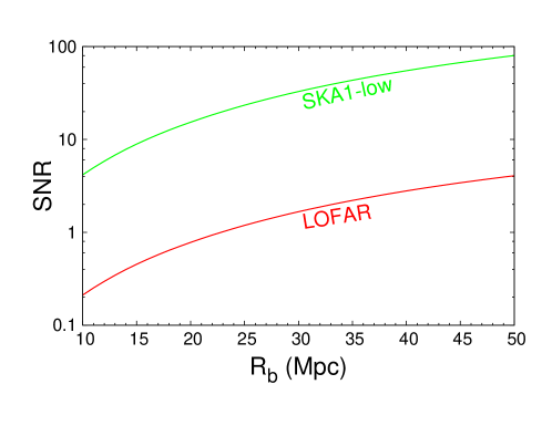
Figure 2: This shows the SNR as a function of comoving radius $R_{b}$ (Mpc) of ionized bubble using the matched filter technique for the model A. Ionized bubbles are assumed to be embedded in uniform IGM with H I fraction $x_{\rm HI}\approx 0.5$. The upper and lower lines show results for the SKA1-low and LOFAR respectively for a total $100$ hr of observations at frequency $165$ MHz corresponding to redshift $z=7.6$. We consider the SKA1-low baseline distribution given in the paper Ghara, Choudhury & Datta (2016). Here, we assume that the SKA1-low has a total $512$ number of antennae each with $35$ m diameters.

4.2 Prospects of detecting bright QSOs

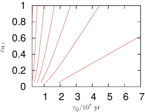
Figure 3: This shows the apparent comoving size of the H ii bubble around a quasar with the ionizing photon emission rate $\dot{N}_{\gamma}=1.3\times 10^{57}\,{\rm sec^{-1}}$, same as ULASJ1120+0641 Mortlock et al. (2011). Different contours from right to left represent $40,\,35,\,30,\,25,\,20,\,15$ and $10$ Mpc.

Figure 4: This shows the estimates (preliminary) of minimum observation time required for $3\sigma$ and $5\sigma$ (left and right panels respectively) detection of the H ii bubble around the quasar ULASJ1120+0641 discovered by Mortlock et al. (2011) using SKA1-low. Different shades of black from dark to light represent $100$, $200$, $400$ and $600$ hr of observations respectively.

We estimate the possibility of detecting the H ii bubble around a quasar using the SKA1-low medium or deep HI 21-cm survey. For this analysis we assume that the quasar under consideration has a spectroscopically confirmed redshift from infrared surveys (similar to the case of Mortlock et al. (2011)), and its location and the luminosity (an extrapolation from the measured spectra) are known. We also assume that the H ii bubble is embedded in uniform IGM with the mean neutral fraction $x_{{\rm H~{}{\sc I}\,}}$. We estimate the total observation time required for the SKA1-low to detect such an H ii region around a high redshift quasar using HI 21-cm observations. We investigate the minimum background $x_{{\rm H~{}{\sc I}\,}}$ and the quasar age required for a statistically significant detection of the H ii bubble. We consider the matched filtering technique described above and introduced in Datta, Bharadwaj & Choudhury (2007) for our analysis. We assume that the quasar under consideration is emitting with a constant ionizing photon luminosity throughout its age and, therefore, growing in size following the model of Yu (2005) (here we consider it to be same as the Mortlock et al. (2011) quasar ULASJ1120+0641 i.e. $\dot{N}_{\gamma}=1.3\times 10^{57}\,{\rm sec^{-1}}$). We consider the apparent anisotropy in the quasar H ii regions shape arising due to the finite light travel time Yu (2005) and include that as the matched filter parameter in our targeted search (Majumdar et al., 2011; Majumdar, Bharadwaj & Choudhury, 2012). The apparent radii of the ionized bubble for different QSO age and the outside $x_{{\rm H~{}{\sc I}\,}}$ are shown in figure 3. We assume that the quasar is located at redshift $z=8$.

For the SKA1-low interferometer we assume $A_{eff}/T_{sys}\approx 500\,{\rm m^{2}\,K^{-1}}$ at $110-160$ MHz with frequency resolution of $\Delta\nu=0.1$ MHz, number of antennas $512$ and a total bandwidth of $32$ MHz, which yields a value of $C^{x}=3.904$ Jy in the following expression of rms of noise Datta, Bharadwaj & Choudhury (2007) contribution in a single baseline

$$\sqrt{\langle\hat{N}^{2}\rangle}=C^{x}\left(\frac{\Delta\nu}{1{\rm MHz}}\right)^{-1/2}\left(\frac{\Delta t}{1sec}\right)^{-1/2}\,.$$ (15)

Using this expression of noise and following the method described in Majumdar, Bharadwaj & Choudhury (2012) we estimate the minimum observation time required for a $3\sigma$ and $5\sigma$ detection of the H ii bubble using the SKA1-low. Note that we do not assume the HI fluctuations outside the targeted bubble due to galaxy generated H ii regions and density fluctuations (Datta et al., 2008, 2012; Majumdar, Bharadwaj & Choudhury, 2012). Figure 4 shows our estimates for SKA1-low. Four different shades of black from dark to light represent $100$, $200$, $400$ and $600$ hr of observations respectively. We find that at least $3\sigma$ detection is possible with $100$ hr of observations if the QSO age and the mean $x_{{\rm H~{}{\sc I}\,}}$ outside the QSO H II region are higher than $10^{7}$ Myr and $0.7$ respectively. If the mean $x_{{\rm H~{}{\sc I}\,}}$ outside the QSO H II region are $\sim 0.4$, $0.3$ and $0.2$, then the total observations time required are $200$, $400$ and $600$ hr respectively when the QSO age is $\sim 10^{7}$ Myr. A $5\sigma$ detection is possible if the QSO age and the outside $x_{{\rm H~{}{\sc I}\,}}$ are at least $\sim 2\times 10^{7}$ Myr and $\sim 0.2$ respectively.

Note that, results presented above and in subsection 4.1 are for very simplistic models and, therefore, should be considered as preliminary one. Detailed investigation needs to be carried out using realistic simulations of the signal, foregrounds and considering observational issues which we aim to address in future.

4.3 Prospects of detecting sources during cosmic dawn

Figure 5: The SNR as a function of different model parameters for the source model mini-QSO and coupling model C. While calculating the dependence of the SNR on a particular parameter, we have fixed the other parameters to their fiducial values. The fiducial value for each parameter is denoted by the vertical dashed line in the corresponding panel. The SNR is calculated using eq. 13 for $1000$ hr of observations with SKA1-low with a bandwidth of $16$ MHz. This figure is taken from Ghara, Choudhury & Datta (2016)

.

In this section, we summarize our results on the prospects of detecting sources during cosmic dawn ( see Ghara, Choudhury & Datta (2016) for more details).

Different panels in Figure 5 show the SNR for the SKA1-low as a function of various parameters related to the source properties such as the stellar mass, overdensity of the surrounding IGM, escape fraction of ionizing photons, age of the source etc. The fiducial values of the parameters are, $M_{\star}=10^{7}M_{\odot}$, $f_{X}=0.05$, $\delta=0$, $f_{\rm esc}=0.1$, $\alpha=1.5$, $t_{\rm age}=20$ Myr. While plotting the dependence of the SNR as a function of a particular parameter, we have kept all the other parameters fixed to their fiducial values. The total observational time and bandwidth are $1000$ hours and $16$ MHz respectively. We find that that the SKA1-low should be able to detect those sources individually with $\sim 9\sigma$ significance at redhift $z=15$ with a total observation of $\sim 1000$ hr.

The strength of the 21-cm signal and corresponding visibility signal increase with the increase in the stellar mass, therefore, the SNR increases with the stellar mass (top left panel). We find that (bottom left panel) the SNR decreases with increase of escape fraction. The amount of Ly-$\alpha$ photons, produced due to the recombination in the ISM, is proportional to $1-f_{\rm esc}$. Thus the Ly-$\alpha$ coupling in the IGM becomes weaker as $f_{\rm esc}$ increases. This results in a smaller absorption region and hence a smaller amplitude of the 21-cm signal. With increase in the age of the source, the size of the 21-cm signal region increases as the photons propagate longer distance and hence the visibility strength at lower baselines as well as the SNR increase, as we can see in the bottom middle panel of Figure 5 . As the signal $\delta T_{b}$ is proportional to the density $(1+\delta)$, the SNR scales linearly with $(1+\delta)$, as presented in the right top panel. We further note that the SNR decreases monotonically with increasing redshift which can be understood from the fact that the system temperature $T_{\rm sys}$ decreases rapidly at lower redshifts. The SNR reduces from $\sim 9$ at $z=15$ to $3$ at $z=20$ for fiducial values of other parameters. We find that the SNR is weakly dependent on the two X-ray parameters i.e, $f_{X}$ and $\alpha$ and we dont show them here.

5 Discussion and conclusions

Detection of individual luminous sources galaxies, QSOs during the epoch of reionization and cosmic dawn through their signature on the HI 21-cm signal is one of the direct approaches to probe the epoch. Current low frequency radio telescopes such as the GMRT, MWA, LOFAR primarily aim to detect the HI 21-cm signal statistically through quantities such as the power spectrum, rms, skewness of the HI 21-cm brightness temperature fluctuations. However, it has been proposed that these experiments may be able to detect individual ionized bubbles around reionization sources using optimum detection techniques such as the matched filter technique (Datta, Bharadwaj & Choudhury, 2007; Datta et al., 2008; Datta, Bharadwaj & Choudhury, 2009; Majumdar et al., 2011; Majumdar, Bharadwaj & Choudhury, 2012; Datta et al., 2012) or in low resolution HI images (Geil & Wyithe, 2008; Zaroubi et al., 2012). With an order of magnitude higher sensitivity, better baseline coverage and better instrument the SKA1-low is expected to detect such objects individually with much less observations time.

In this paper, we summarize our previous and ongoing works on this issue and present some preliminary results on the prospects of detecting individual sources during reionization and cosmic dawn using SKA1-low HI 21-cm maps. While calculating the HI 21-cm signal around individual sources we consider three scenarions: (i) The first scenario, named model A, assumes that the HI spin temperature is fully with the IGM kinetic temperature through Ly-$\alpha$ coupling and both the temperatures are much higher than the background CMB temperature. This is a likely scenario when the Universe is already $\sim 10-20\%$ ionized or the time period subsequent to that. The central source creates a spherical ionized bubble which is embedded in a uniform fully neutral (or partially neutral) medium. (ii) In the second scenario, named model B, we assume that the HI spin temperature is completely coupled with the IGM kinetic temperature. Additionally, we assume that the DM halo hosts a X-ray source its centre and calculate the HI spin temperature and the IGM kinetic temperature profile around it. (iii) Model C which is our third model, calculates, self-consistently, the Ly-$\alpha$ coupling, heating, ionisation profile around the source. This is believed to be the case at very early stages of the cosmic dawn. We discuss various features in the differential brightness temperature profile around the central source in these three models. Subsequently, we calculate, analytically, the corresponding visibility signal and discuss its various features for the above three models.

We propose two visibility based methods for detecting such signal around individual sources: one based on the matched filter formalism we developed (Datta, Bharadwaj & Choudhury, 2007; Datta et al., 2008, 2012) and the other relies on simply combining visibility signal from all baselines and frequency channels (Ghara, Choudhury & Datta (2016)). We apply the first method to the model A i.e, to spherical ionized bubble model during the reionization epoch. We find that the SKA1-low should be able to detect ionized bubbles of radius $R_{b}\gtrsim 10$ Mpc with $\sim 100$ hr of observations at redshift $z\sim 8$ provided that the mean outside neutral fraction $x_{{\rm H~{}{\sc I}\,}}\gtrsim 0.5$. Higher observation time would be required for lower neutral fraction. We also investigate the possibility of detecting HII regions around known bright QSOs such as around ULASJ1120+0641 discovered by Mortlock et al. (2011). We find that a $5\sigma$ detection is possible with $600$ hr of SKA1-low observations if the QSO age and the outside $x_{{\rm H~{}{\sc I}\,}}$ are at least $\sim 2\times 10^{7}$ Myr and $\sim 0.2$ respectively.

Finally, we study the prospects of detecting the very first X-ray and Ly-$\alpha$ sources in model B and C during the cosmic dawn. We consider the mini-QSOs as a source of X-ray photons. We find that around $\sim 1000$ hr would be required to detect those sources individually with SKA1-low. We also study how the SNR changes with various parameters related to the source properties such as the stellar mass, escape fraction of ionizing photons, X-ray to UV luminosity ratio, age of the source and the overdensity of the surrounding IGM.

Finally, we emphasise that the work we present and discuss here should be treated as a preliminary one. Further work using detailed simulations needs to be done to understand the signal properties. Detail investigation is also necessary in order to understand the impact of the foreground subtraction, data calibration, ionospheric turbulence, RFI mitigation effects etc. We plan to adress some of these issues in future.

References

- Barkana & Loeb (2005) Barkana, R., & Loeb, A. 2005, ApJL, 624, L65
- Bharadwaj & Ali (2004) Bharadwaj, S., & Ali, S. S. 2004, MNRAS, 352, 142
- Bouwens et al. (2015) Bouwens R. J., et al., 2015, ApJ, 803, 34
- Datta, Choudhury & Bharadwaj (2007) Datta, K. K., Choudhury, T. R., & Bharadwaj, S. 2007, MNRAS, 378, 119
- Datta, Bharadwaj & Choudhury (2007) Datta, K. K., Bharadwah, S., & Choudhury, T. R. (2007), MNRAS
- Datta et al. (2008) Datta, K. K., Majumdar, S., Bharadwaj, S., & Choudhury, T. R., 2008,MNRAS, 391, 1900
- Datta, Bharadwaj & Choudhury (2009) Datta, K. K., Bharadwaj, S., & Choudhury, T. R. 2009, MNRAS, 399, L132
- Datta et al. (2012) Datta, K. K., Friedrich, M. M., Mellema, G., Iliev, I. T., & Shapiro, P. R. 2012, MNRAS, 424, 762
- De Souza et al. (2013) De Souza R. S., Ishida E. E. O., Johnson J. L., Whalen D. J., Mesinger A., 2013, MNRAS, 436, 1555
- De Souza et al. (2014) De Souza R. S., Ishida E. E. O., Whalen D. J., Johnson J. L., Ferrara A., 2014, MNRAS, 442, 1640
- Ellis et al. (2013) Ellis R. S., et al., 2013, ApJ, 763, L7
- Fan et al. (2006) Fan X., et al., 2006, AJ, 132, 117
- Geil & Wyithe (2008) Geil, P. M., & Wyithe, J. S. B. 2008, MNRAS, 386, 1683
- Ghara, Choudhury & Datta (2016) Ghara, R., Choudhury, T. R., & Datta, K. K. 2016, MNRAS, 460, 827
- Ghara et al. (2016) Ghara, R., Choudhury, T. R., Datta, K. K., & Choudhuri, S. 2016, MNRAS (in press), arXiv:1607.02779
- Hu et al. (2010) Hu E. M., Cowie L. L., Barger A. J., Capak P., Kakazu Y., Trouille L., 2010, ApJ, 725, 394
- Kashikawa et al. (2011) Kashikawa N., et al., 2011, ApJ, 734, 119
- Majumdar et al. (2011) Majumdar, S., Bharadwaj, S., Datta, K., K., & Choudhury, T. R. 2011, MNRAS, 413, 1409
- Majumdar, Bharadwaj & Choudhury (2012) Majumdar, S., Bharadwaj, S., & Choudhury, T. R. 2012, MNRAS, 426, 3178
- Malloy & Lidz (2013) Malloy, M., & Lidz, A. 2013, ApJ, 767, 68
- Mellema et al. (2013) Mellema, G., Koopmans, L. V. E., Abdalla, F. A., et al. 2013, Experimental Astronomy, 36, 235
- Mellema et al. (2015) Mellema, G., Koopmans, L., Shukla, H., et al. 2015, Advancing Astrophysics with the Square Kilometre Array (AASKA14), 10
- Mortlock et al. (2011) Mortlock, D., J., et al. 2011, Nature, 474, 7353
- Ouchi et al. (2010) Ouchi M., et al., 2010, ApJ, 723, 869
- Venamans et al. (2015) Venemans B. P., et al., 2015, ApJ, 801, L11
- Yu (2005) Yu, Q. 2005, ApJ, 623, 683
- Zackrisson et al. (2011) Zackrisson E., Rydberg C.-E., Schaerer D., ¨ Ostlin G., Tuli M., 2011, ApJ, 740, 13
- Zaroubi et al. (2012) Zaroubi, S., de Bruyn, A. G., Harker, G., et al. 2012, MNRAS, 425, 2964