Sound Probabilistic with Projection

Abstract

We present an improved method for a sound probabilistic estimation of the model count of a boolean formula under projection. The problem solved can be used to encode a variety of quantitative program analyses, such as concerning security of resource consumption. We implement the technique and discuss its application to quantifying information flow in programs.

1 Introduction

The problem is concerned with counting the number of models of a boolean formula. Since is a computationally difficult problem, not only exact but also approximative solutions are of interest. A powerful approximation method is probabilistic approximation, making use of random sampling. We call a probabilistic approximation method sound when the probability and magnitude of the sampling-related error can be bounded a priory. A prominent recent development in sound probabilistic is ApproxMC [2].

In this paper we present ApproxMC-p, an improved method and a tool for sound probabilistic with projection. Just as ApproxMC, which it enhances, ApproxMC-p belongs to the category of $(\epsilon,\delta)$ counters. In this context, the parameter $\epsilon$ represents the tolerance and $1-\delta$ the confidence of the result. For example, choosing $\epsilon=0.1$ and $\delta=0.14$ implies that the computed result provably lies with a probability of 86% between the $0.9$-fold and the $1.1$-fold of the correct result. Both parameters can be configured by the user.

An enticing application of solvers is quantitative program analysis, which often requires establishing cardinality of sets defined in terms of the set of reachable program states. Reducing an analysis to has the advantage that one can use a variety of established reasoning techniques. At the same time, it is reasonably easy to represent behavior of intricate low-level programs in boolean logic. Yet, alone is typically not sufficient for this purpose—one needs a way to reason about program reachability. In logic, this reasoning corresponds to projection. If a boolean formula encodes a relation (e.g., a transition relation on states), then computing the image or the preimage of the relation is a projection operation.

ApproxMC-p takes as input a boolean formula in conjunctive normal form together with a projection scope (a set of variables) and the parameters $\epsilon$ and $\delta$ and estimates the number of models of the formula projected on the given scope. Of course, by setting the scope to encompass all variables in the logical signature, one can use ApproxMC-p as a non-projecting solver.

The specific contributions of this paper are the following:

First, we materially improve the performance of ApproxMC, in particular its base confidence. Probabilistic counters meet confidence demands above the base confidence by repeating the estimation. We reduce the number of repetitions for confidence values above 0.6 by about an order of magnitude on average. Furthermore, we reduce, for one repetition, the number of SAT solver queries by at least $15\%$. A detailed comparison is presented in Section 3.1.

Second, we combine probabilistic model counting with projection, even though the ideas behind this combination are not completely new. A particular special case has previously appeared in [3] in the context of uniform model sampling. There, the formula $\varphi$ is treated by considering only its projection on the independent support. An independent support is a subset of variables that uniquely determines the truth value of the whole formula. It is often known from the application domain. For formulas generated from deterministic programs, for instance, the independent support is the preimage of the transition relation. Our approach is more general in that we explicitly consider projection on arbitrary scopes.

Third, we implement the method and map its pragmatics. We show that ApproxMC-p is effective for large formulas with a large number of models, which may make other tools run out of time or memory. Finally, we discuss applications of ApproxMC-p to quantifying information flow in programs.

1.1 Logical Foundations

We assume that logical formulas are built from usual logical connectives ($\wedge$, $\vee$, $\neg$, etc.) and propositional variables from some vocabulary set $\Sigma$. A model is a map assigning every variable in $\Sigma$ a truth value. A given model $M$ can be homomorphically extended to give a truth value to a formula $\varphi$ according to standard rules for logical connectives. We call a model $M$ a model of $\varphi$, if $M$ assigns $\varphi$ the value True. A formula $\varphi$ is satisfiable if it has at least one model, and unsatisfiable otherwise.

In the following, we assume that $\Sigma$ and $\Delta$ are vocabularies with $\Delta\subseteq\Sigma$. A $\Sigma$-entity (i.e., formula or model) is an entity defined (only) over vocabulary from $\Sigma$. We assume that $\varphi$ denotes a $\Sigma$-formula and $M$ a $\Sigma$-model. With $\mathit{vocab}(\varphi)$ we denote the vocabulary actually appearing in $\varphi$.

With $\mathop{models}_{\Sigma}({\varphi})$ we denote the set of all models of $\varphi$. If $\varphi$ is unsatisfiable, the result is the empty set $\emptyset$. With $|\varphi|$ we denote the number of models of the formula $\varphi$ (i.e., $|\varphi|=|\mathop{models}_{\Sigma}({\varphi})|$). With ${\left.\kern-1.2ptM\vphantom{\big{|}}\right|_{\Delta}}$ we denote the $\Delta$-model that coincides with the $\Sigma$-model $M$ on the vocabulary $\Delta$.

With ${\left.\kern-1.2pt\varphi\vphantom{\big{|}}\right|_{\Delta}}$ we denote the projection of $\varphi$ on $\Delta$, i.e., the strongest $\Delta$-formula that, when interpreted as a $\Sigma$-formula, is entailed by $\varphi$. The projected formula ${\left.\kern-1.2pt\varphi\vphantom{\big{|}}\right|_{\Delta}}$ says the same things about $\Delta$ as $\varphi$ does—but nothing else. Projection of $\varphi$ on $\Delta$ can be seen as quantifying the $\Sigma\setminus\Delta$-variables in $\varphi$ existentially and then eliminating the quantifier (i.e., computing an equivalent formula without it). Furthermore, $\mathop{models}_{\Delta}({{\left.\kern-1.2pt\varphi\vphantom{\big{|}}\right|_{\Delta}}})=\{{\left.\kern-1.2ptM\vphantom{\big{|}}\right|_{\Delta}}\mid M\in\mathop{models}_{\Sigma}({\varphi})\}$.

1.2 Related Work

A number of exact boolean model counters exist. Counters such as Dsharp [18] and sharpSAT [23] are based on compiling the formula to the Deterministic Decomposable Negation Normal Form (d-DNNF). They are geared toward formulas with a large number of models but tend to run out of memory as formula size increases. An extension of the above with projection has been presented in [12]. Another class of exact counters implements variations of the blocking clause approach (cf. Section 2.3) and includes tools such as sharpCDCL [12] and CLASP [6]. The counters in this class are often already projection-capable. They can deal with very large formulas (hundreds of megabyte in DIMACS format) but are challenged by large model counts.

The probabilistic counters can be divided into three classes. The first class are the already mentioned $(\epsilon,\delta)$ counters. These counters were originally introduced by Karp and Luby [10] to count the models of DNF formulas. They guarantee with a probability of at least $1-\delta$ that the result will be between $1-\epsilon$ and $1+\epsilon$ times the actual number of models. An instantiation of this class for CNF formulas is ApproxMC [2].

For reasons unknown to us, ApproxMC deviates from the original definition [10] of an $(\epsilon,\delta)$ counter by defining the tolerable result interval as $\left[|\varphi|/(1+\epsilon),|\varphi|\cdot(1+\epsilon)\right]$. We adhere to the original definition of the tolerable interval, that is $\left[|\varphi|\cdot(1-\epsilon),|\varphi|\cdot(1+\epsilon)\right]$. We discuss the differences between ApproxMC and our work in detail in Section 3.1.

The second class are lower/upper bounding counters. These counters drop the tolerance guarantee and compute an upper/lower bound for the number of models that is correct with a probability of at least $1-\delta$ (for a user-specified $\delta$). Examples are BPCount [13], MiniCount [13], MBound [8] and Hybrid-MBound [8].

The third class are guarantee-less counters. These counters provide no formal guarantees but can be very good in practice. Examples are ApproxCount [25], SearchTreeSampler [5], SE [19] and SampleSearch [7].

2 Method

2.1 The Idea

The intuitive idea behind ApproxMC-p is to partition the set $\mathop{models}_{\Sigma}({{\left.\kern-1.2pt\varphi\vphantom{\big{|}}\right|_{\Delta}}})$ into buckets so that each bucket contains roughly the same number of models. The partitioning is based on strongly universal hashing and is, surprisingly, attainable with high probability without any knowledge about the structure of the set of models. The count of $\mathop{models}_{\Sigma}({{\left.\kern-1.2pt\varphi\vphantom{\big{|}}\right|_{\Delta}}})$ can then be estimated as the count of models in one bucket multiplied with the number of buckets.

More technically, ApproxMC-p is based on Chernoff-Hoeffding bounds, one of the so called concentration inequalities. This theorem (Theorem 2.6) limits the probability that the sum of random variables – under certain side conditions – deviates from its expected value. To apply the theorem we make use of a trick common in counting, namely that set cardinality can be expressed as the sum of the membership indicator function over the domain.

Assume that we fixed the set of buckets $B$, a way of distributing models of $\varphi$ into buckets by means of a hash function $h$, and distinguished one particular bucket. We now associate each model with an indicator variable (a random variable over the hash function $h$) that is $1$ iff the model is within the distinguished bucket and $0$ otherwise. Hence, for a given hash function $h$, the sum of all those indicator variables is exactly the amount of models within the distinguished bucket. We will determine this value by means of a deterministic model counting procedure Bounded#SAT (Section 2.3).

On the other hand, the expected number of models in the bucket when choosing $h$ randomly from the class of strongly $r$-universal hash functions (Section 2.2) is ${|\mathop{models}_{\Sigma}({{\left.\kern-1.2pt\varphi\vphantom{\big{|}}\right|_{\Delta}}})|}/{B}$. The Chernoff-Hoeffding theorem tells us that the measured and the expected values are probably close and allows us to estimate $|\mathop{models}_{\Sigma}({{\left.\kern-1.2pt\varphi\vphantom{\big{|}}\right|_{\Delta}}})|$.

We first explain how to build an $(\epsilon,\delta)$ counter this way for a fixed confidence $1-\delta\approx 0.86$ (Section 2.4). Then, we generalize this result to arbitrary higher confidences (Section 2.5).

The idea behind adding projection capability is to hash partial models (i.e., models restricted to the projection scope) and to use a projection-capable version of Bounded#SAT. To separate concerns, we postpone discussing projection until Section 2.6. The algorithms we present in the following are capable of projection, but we begin with a tacit assumption that they are always invoked with the value of the scope $\Delta=\Sigma$, i.e., in a non-projecting fashion. We will show that this assumption is superfluous in Section 2.6.

2.2 Strongly $r$-Universal (aka $r$-Wise Independent) Hash Functions

The key to distributing models of a formula into a number of buckets filled roughly equally is to apply strongly $r$-universal hashing [24] (also known as $r$-wise independent or, simply, $r$-independent hashing). Every concrete strongly $r$-universal hash function depends on a parameter. By choosing the parameter at random, one can make a good distribution of values into hash buckets likely, even when the keys are under adversarial control.

Definition 2.1 (strongly $r$-universal hash functions [24]).

Let $K$ be some universe from which the keys to be hashed are drawn, and $B$ a set of buckets (hash values). A family of hash functions $H=\{h\colon K\to B\}$ is strongly $r$-universal, iff for any $h\in H$ chosen uniformly at random, the hash values of any $r$-tuple of distinct keys $(k_{1},\ldots,k_{r})\in K^{r}$ are independent random variables, i.e., for any $r$-tuple of (not necessarily distinct) values $(v_{1},\ldots,v_{r})\in B^{r}$

$$\Pr_{h\in H}\big{[}h(k_{1})=v_{1}\wedge\ldots\wedge h(k_{r})=v_{r}\big{]}=\left(\frac{1}{|B|}\right)^{r}\enspace.$$

In the following, we are interested in families of strongly $r$-universal hash functions with $K=\mathbb{Z}_{2}^{n}$ and $B=\mathbb{Z}_{2}^{m}$. We denote any such family as $H(n,m,r)$. Functions $h\in H(n,m,r)$ can be used to distribute models with $n$ variables into $2^{m}$ buckets. While we keep the rest of the presentation generic, our implementation resorts to a particular family $H_{\mathit{xor}}(n,m,3)$ of such functions with $r=3$. Any discussion of concrete values refers to this family and the corresponding degree of strong universality. Note that the construction operates on $\mathbb{Z}_{2}\cong\{0,1\}$, and that addition on $\mathbb{Z}_{2}$ corresponds to exclusive or (boolean XOR), while multiplication on $\mathbb{Z}_{2}$ corresponds to conjunction (boolean AND). Otherwise, the usual matrix and vector arithmetic rules apply.

Construction 2.2 (Hash function family $H_{\mathit{xor}}(n,m,3)$).

Let $n$ and $m$ be arbitrary natural numbers. Any $m\cdot(n+1)$ values $b_{1;0},\ldots,b_{m;n}\in\mathbb{Z}_{2}$ define a hash function $h\colon\mathbb{Z}_{2}^{n}\to\mathbb{Z}_{2}^{m}$ by

$$\bar{z}\mapsto\begin{pmatrix}b_{1;0}\\ \vdots\\ b_{m;0}\end{pmatrix}\oplus\begin{pmatrix}b_{1;1}&\cdots&b_{1;n}\\ \vdots&\ddots&\vdots\\ b_{m;1}&\cdots&b_{m;n}\end{pmatrix}\otimes\begin{pmatrix}z_{1}\\ \vdots\\ z_{n}\end{pmatrix}\enspace.$$

We denote the class of all such hash functions as $H_{\mathit{xor}}(n,m,3)$.

Theorem 2.3 ([9]).

The hash function class $H_{\mathit{xor}}(n,m,3)$ is strongly $3$-universal.

By sampling $b_{1;0},\ldots,b_{m;n}$ uniformly from $\mathbb{Z}_{2}$, we can sample uniformly from $H_{\mathit{xor}}(n,m,3)$.

Construction 2.4.

Let $h\in H_{\mathit{xor}}(n,m,3)$ be a hash function. Fixing its output induces a predicate on its inputs. In this paper, we will consider for each $h$, the predicate $h(\bar{z})=1^{m}$. This semantical predicate can be represented syntactically as a formula of propositional logic built from $m$ XOR clauses:

$$\big{(}b_{1;0}\oplus(b_{1;1}\wedge z_{1})\oplus\ldots\oplus(b_{1;n}\wedge z_{n})\big{)}\wedge\ldots\wedge\big{(}b_{m;0}\oplus(b_{m;1}\wedge z_{1})\oplus\ldots\oplus(b_{m;n}\wedge z_{n})\big{)}\enspace.$$ (1)

Construction 2.5.

Given a hash function $h$, we use the notation $\varphi_{h}$ to denote the conjunction of a formula $\varphi$ with the clause representation (1) of the predicate induced by $h$.

For presentation purposes, we assume w.l.o.g. that $\Sigma=\{z_{1},\ldots,z_{n}\}$ and $\Delta=\{z_{1},\ldots,z_{|\Delta|}\}$ in the following. Our implementation does not have this limitation.

2.3 Helper Algorithm Bounded#SAT: Iterative Model Enumeration

1

2$k\leftarrow 0$ ;

3 $M\leftarrow\textsc{SAT}(\varphi)$ ;

4 while $(M\neq\bot)\wedge(k<n)$ do

5       $k\leftarrow k+1$ ;

6       $\varphi\leftarrow\varphi\wedge(\Delta\not\simeq{\left.\kern-1.2ptM\vphantom{\big{|}}\right|_{\Delta}})$ ;

7       $M\leftarrow\textsc{SAT}(\varphi)$ ;

8      

9 end while

return $k$

Algorithm 1 Bounded#SAT($\varphi,\Delta,n$)

To enumerate the models in a single bucket we are using the well-known algorithm Bounded#SAT (Algorithm 1). Given a formula $\varphi$, a projection scope $\Delta\subseteq\Sigma$, and a bound $n\geqslant 0$, the algorithm enumerates up to $n$ models of ${\left.\kern-1.2pt\varphi\vphantom{\big{|}}\right|_{\Delta}}$, i.e., it returns $\mathop{min}(|{\left.\kern-1.2pt\varphi\vphantom{\big{|}}\right|_{\Delta}}|,n)$. The algorithm makes use of the oracle $\textsc{SAT}(\cdot)$, which for a CNF formula returns either a model or $\bot$, in case none exists. Bounded#SAT works by repeatedly asking the oracle for a model $M$ of $\varphi$, and extending $\varphi$ with a blocking clause $(\Delta\not\simeq{\left.\kern-1.2ptM\vphantom{\big{|}}\right|_{\Delta}})$ ensuring that any model found later must differ in at least one $\Delta$-variable. The formula $\Delta\not\simeq{\left.\kern-1.2ptM\vphantom{\big{|}}\right|_{\Delta}}$ can be constructed as $\bigvee_{v\in\Delta}\mathit{flip}(v,M)$, where $\mathit{flip}(v,M)=v$, if $M(v)=\textsc{False}$, and $\mathit{flip}(v,M)=\neg v$, if $M(v)=\textsc{True}$. The algorithm is widely-known as part of the automated deduction lore. We have reported on our experiences with using it for quantitative information flow analysis in [12].

2.4 Counting with a Fixed Confidence of 86%

1

2$n:=|\Delta|$ ;

3 $\mathit{pivot}:=\left\lceil\frac{2\cdot r\cdot(1+\epsilon)\cdot\sqrt[3]{e}}{\epsilon^{2}}\right\rceil$ ;

4 $m\leftarrow 0$ ;

5 repeat

6       $m\leftarrow m+1$ ;

7      

8      $h\overset{\text{random}}{\leftarrow}H(n,m,r)$ ;

       $c\leftarrow$ Bounded#SAT($\varphi_{h},\Delta,\mathit{pivot}+1$) ;

        // $c=\min(|{\left.\kern-1.2pt\varphi_{h}\vphantom{\big{|}}\right|_{\Delta}}|,\mathit{pivot}+1)$

9      

10until $c\leq\mathit{pivot}\;\vee\;m>\left\lceil\log_{2}\left(\frac{(1+\epsilon)\cdot 2^{n}}{\mathit{pivot}}\right)\right\rceil$;

11

return $c\cdot 2^{m}$ ;

  // Count of one bucket times number of buckets

Algorithm 2 Core($r$, $\varphi$, $\Delta$, $\epsilon$)

We first explain how to build an $(\epsilon,\delta)$ counter for a fixed confidence $1-\delta\approx 0.86$: the algorithm Core. The number stems from the probability of deviation $e^{\lfloor-r/2\rfloor}\approx 0.14$ for $r=3$ in the following theorem.

Theorem 2.6 (Chernoff-Hoeffding bounds with limited independence [20]).

If $\Gamma$ is the sum of $r$-wise independent random variables, each of which is confined to the interval $[0,1]$, then the following holds for $\mu:=E[\Gamma]$ and for every $\epsilon\in[0,1]$: If $r\leq\lfloor\epsilon^{2}\cdot\mu/\sqrt[3]{e}\rfloor$ then $\Pr\left[|\Gamma-\mu|\geq\epsilon\cdot\mu\right]\leq e^{\lfloor-r/2\rfloor}$.

Corollary 2.7.

If $r\leq\lfloor\epsilon^{2}\cdot\mu/\sqrt[3]{e}\rfloor$, then $\Pr\left[(1-\epsilon)\cdot\mu\leq\Gamma\leq(1+\epsilon)\cdot\mu\right]\geq 1-e^{\lfloor-r/2\rfloor}$.

Construction 2.8.

Let $h$ be chosen randomly from $H(n,m,r)$. For each $M\in\mathop{models}_{\Sigma}({\varphi})$, we define an integer random variable $\gamma_{M}$ (random over $h$) such that

$$\gamma_{M}:=\begin{cases}1,\qquad\text{if }h(M)=1^{m}\\ 0,\qquad\text{otherwise.}\end{cases}$$

The sum of these random variables we denote by $\Gamma:=\sum_{M\in\mathop{models}_{\Sigma}({\varphi})}\gamma_{M}$.

Clearly, $\Gamma=|\varphi_{h}|$ (cf. Construction 2.5).

Lemma 2.9.

For the above construction, the following holds:

1. The variables $\gamma_{M}$ are $r$-wise independent.

2. For any $M\in\mathop{models}_{\Sigma}({\varphi})$, $\Pr[\gamma_{M}=1]=1/2^{m}$.

The expectation of $\Gamma$ (over $h$) is thus $\mu:=E[\Gamma]=\sum_{M\in\mathop{models}_{\Sigma}({\varphi})}E[\gamma_{M}]=\sum_{M\in\mathop{models}_{\Sigma}({\varphi})}2^{-m}\cdot 1=|\varphi|\cdot 2^{-m}$. Substituting these values into Corollary 2.7, we obtain:

Lemma 2.10 (Models in a hash bucket).

Let $\varphi\in\text{Fml}_{\Sigma}$, $n:=|\Sigma|$, $\epsilon\in[0,1]$, let $m\in\mathbb{N}$ with $m\leq\lfloor\log_{2}(|\varphi|\cdot\epsilon^{2}/(r\cdot\sqrt[3]{e}))\rfloor$, $h\in H(n,m,r)$ a randomly chosen strongly $r$-universal hash function. It holds:

$$\Pr\left[(1-\epsilon)\cdot\frac{|\varphi|}{2^{m}}\leq|\varphi_{h}|\leq(1+\epsilon)\cdot\frac{|\varphi|}{2^{m}}\right]\geq 1-e^{\lfloor-r/2\rfloor}\enspace.$$

One could think that this lemma is sufficient for estimating $|\varphi|$ by determining $|\varphi_{h}|$ for some $m$ (e.g., with Bounded#SAT), but, unfortunately, the upper bound on the admissible values of $m$ depends on $|\varphi|$, the very value we are trying to estimate. This fact forces us to search for a “good” value of $m$ in Core (Lines 2–2). The search proceeds in ascending order of $m$ for reasons of soundness, which will be explained in the main theorem below. At the same time, smaller values of $m$ correspond to larger values of $|\varphi_{h}|$, which may be infeasible to count (for $m=0$, for instance, $\varphi_{h}=\varphi$). We thus introduce the counting upper bound $\mathit{pivot}$, which only depends on the tolerance and is defined in Core. The search terminates successfully when $|\varphi_{h}|\leq\mathit{pivot}$. We show that this search criterion does not reduce the probability of correct estimation (Theorem 2.12).

Lemma 2.11.

Core terminates for all inputs.

Proof.

The loop has two exit conditions combined in a disjunction (Line 2). Since $m$ is monotonically increasing, the second exit condition guarantees termination. Note that the second exit condition makes use of the fact that $|\varphi|\leq 2^{n}$ and is essentially an emergency stop. It does not, in general, entail that the algorithm returns a tolerable estimation. This is not a problem, as we will show that the first exit condition (which implies an estimation within desired tolerance) terminates the loop sufficiently often for the desired confidence level. ∎

Theorem 2.12 (Main result).

For $\epsilon\in(0,1]$ algorithm Core returns with a probability of at least $1-e^{\lfloor-r/2\rfloor}$ a value within $\left[(1-\epsilon)\cdot|\varphi|,(1+\epsilon)\cdot|\varphi|\right]$.

Proof.

It is easy to see that $c=\min(|\varphi_{h}|,\mathit{pivot}+1)$ is an invariant of the loop in Core. If the exit condition $c\leq\mathit{pivot}$ comes to hold, the invariant dictates that Core returns $2^{m}\cdot|\varphi_{h}|$.

We now show that there is at least one iteration of the loop (indexed by $m=m^{\prime}$) such that with a probability of at least $1-e^{\lfloor-r/2\rfloor}$ the following is true: the exit condition $c\leq\mathit{pivot}$ holds and the return value $2^{m^{\prime}}\cdot|\varphi_{h}|\in\left[(1-\epsilon)\cdot|\varphi|,(1+\epsilon)\cdot|\varphi|\right]$. But first, we interrupt the proof for a lemma.

Lemma 2.13.

For the given choice of $\mathit{pivot}$, there exists $m^{\prime}$ such that:

$$\lceil\log_{2}((1+\epsilon)\cdot|\varphi|/\mathit{pivot})\rceil\leq m^{\prime}$$ (2)

$$m^{\prime}\leq\lfloor\log_{2}(|\varphi|\cdot\epsilon^{2}/(r\cdot\sqrt[3]{e}))\rfloor\enspace.$$ (3)

Proof.

It is straightforward to show that $\lceil\log_{2}((1+\epsilon)\cdot|\varphi|/\mathit{pivot})\rceil\leq\lfloor\log_{2}(|\varphi|\cdot\epsilon^{2}/(r\cdot\sqrt[3]{e}))\rfloor$. ∎

Condition (3) on $m^{\prime}$ fulfills the precondition of Lemma 2.10 and thus entails

$$\Pr\left[(1-\epsilon)\cdot\frac{|\varphi|}{2^{m^{\prime}}}\leq|\varphi_{h}|\leq(1+\epsilon)\cdot\frac{|\varphi|}{2^{m^{\prime}}}\right]\geq 1-e^{\lfloor-r/2\rfloor}$$ (4)

which together with condition (2), which is equivalent to $(1+\epsilon)\cdot\frac{|\varphi|}{2^{m^{\prime}}}\leq\mathit{pivot}$, gives

$$\Pr\left[(1-\epsilon)\cdot\frac{|\varphi|}{2^{m^{\prime}}}\leq|\varphi_{h}|\leq(1+\epsilon)\cdot\frac{|\varphi|}{2^{m^{\prime}}}\leq\mathit{pivot}\right]\geq 1-e^{\lfloor-r/2\rfloor}$$ (5)

resp.

$$\Pr\left[(1-\epsilon)\cdot\frac{|\varphi|}{2^{m^{\prime}}}\leq|\varphi_{h}|\leq(1+\epsilon)\cdot\frac{|\varphi|}{2^{m^{\prime}}}\;\wedge\;|\varphi_{h}|\leq\mathit{pivot}\right]\geq 1-e^{\lfloor-r/2\rfloor}\enspace.$$

Since we are incrementing $m$ during search, the last equation implies that both loop termination and result quality are likely at some point. We also note that an earlier termination with $m<m^{\prime}$ is not problematic, since result quality hinges on condition (3), which is an upper bound on $m$. ∎

2.5 Scaling to Arbitrary Confidence

1

2$t:=\min\left(\left\{n\in\mathbb{N}:\delta\geq\sum_{k=\lceil n/2\rceil}^{n}\binom{n}{k}\cdot e^{\lfloor-r/2\rfloor\cdot k}\cdot(1-e^{\lfloor-r/2\rfloor})^{n-k}\right\}\right)$ ;

3 $\mathit{pivot}:=\left\lceil\frac{2\cdot r\cdot(1+\epsilon)\cdot\sqrt[3]{e}}{\epsilon^{2}}\right\rceil$ ;

4

5$c\leftarrow$ Bounded#SAT($\varphi,\Delta,\mathit{pivot}+1$) ;

6 if $c\leq\mathit{pivot}$ then

       return $c$ ;

        // solution is exact with confidence $1$

7      

8else

       $\mathit{samples}\leftarrow$ repeat($t$, Core($r$, $\varphi$, $\Delta$, $\epsilon$)) ;

        // do Core $t$ times

9      

10      return median($\mathit{samples}$) ;

11      

12 end if

Algorithm 3 Main($r$, $\varphi$, $\Delta$, $\epsilon$, $\delta$)

Since Core returns the correct result with a probability of approx. $0.86>0.5$, it is possible to amplify the confidence by repeating the experiment. This is what algorithm Main does. To prove its correctness (Theorem 2.15), a technical lemma is needed first.

Lemma 2.14 (Biased coin tosses and related estimations).

Let $p:=\Pr[\text{head}]$ be the probability of tossing head with a biased coin.

1. The probability to toss $m$ times head in $n\geqslant m$ independent coin tosses is $\binom{n}{m}\cdot p^{m}\cdot(1-p)^{n-m}$

2. The probability of tossing at least $m$ heads is: $\sum_{k=m}^{n}\binom{n}{k}\cdot p^{k}\cdot(1-p)^{n-k}$

3. (Geometric series) For every non-negative integer $n$: $\sum_{k=0}^{n}x^{k}=\frac{1-x^{n+1}}{1-x}$

4. The probability to toss at least $m=\lceil n/2\rceil$ times head for $p\in[0,1/2]$ can be bounded from above:

   $$\sum_{k=\lceil n/2\rceil}^{n}\binom{n}{k}\cdot p^{k}\cdot(1-p)^{n-k}\leq\frac{1-p}{1-2\cdot p}\cdot\left(\sqrt{4\cdot p\cdot(1-p)}\right)^{n}\enspace.$$

Theorem 2.15 (Theorem 3 in [2]).

Let $\varphi$ be a formula, $\delta$ and $\epsilon$ parameters in $(0,1]$, and $\tilde{c}$ an output of $\textsc{Main}(r,\varphi,\epsilon,\delta)$. Then $\Pr\big{[}(1-\epsilon)\cdot|\varphi|\leqslant\tilde{c}\leqslant(1+\epsilon)\cdot|\varphi|\big{]}\geqslant 1-\delta$.

Proof.

If $|\varphi|\leq\mathit{pivot}$, Main returns the exact solution (Algorithm 3, Line 3). If not, the algorithm returns the median $\tilde{c}$ of $t$ probabilistic estimations ($t$ is defined in Algorithm 3, Line 3). The goal is to show that the probability of $\tilde{c}$ being outside the tolerance is at most $\delta$.

A necessity for $\tilde{c}$ being outside the tolerance is that at least $\lceil t/2\rceil$ of the estimations of Core are outside the tolerance, due to the definition of the median. The probability that a single estimation of Core is outside the tolerance is at most $e^{\lfloor-r/2\rfloor}$ by Theorem 2.12. Now, the probability to have at least $\lceil t/2\rceil$ estimations (out of $t$ estimations in total) outside the tolerance can be seen as the probability to toss at least $\lceil t/2\rceil$ times head in a series of $t$ coin tosses where $\Pr[\text{head}]=e^{\lfloor-r/2\rfloor}$. By Lemma 2.14 b, this probability is:

$$\sum_{k=\lceil t/2\rceil}^{t}\binom{t}{k}\cdot e^{\lfloor-r/2\rfloor\cdot k}\cdot\left(1-e^{\lfloor-r/2\rfloor}\right)^{t-k}\enspace.$$

Due to the choice of $t$, this probability is smaller than $\delta$. The existence of $t$ is ensured, because $t$ can be bounded from above per Lemma 2.14 d:

$$t\leq\max\left(1,\left\lceil\log_{\sqrt{4\cdot e^{\lfloor-r/2\rfloor}\cdot(1-e^{\lfloor-r/2\rfloor})}}\left(\delta\cdot\frac{1-2\cdot e^{\lfloor-r/2\rfloor}}{1-e^{\lfloor-r/2\rfloor}}\right)\right\rceil\right)\enspace.$$

The value of $t$ can be (pre-)computed by a simple search (see Table 2). ∎

Note 2.16 (Leap-frogging).

We observe that every repetition of Core begins the search for the proper number of buckets with $m=1$. It is natural to ask if the repeated search can be abridged. In [2], a heuristic called leap-frogging is proposed. Leap-frogging tracks the successful values of $m$ (i.e., the ones upon termination) as Core is repeated. After a short stabilization period, subsequent runs of Core begin the search not with $m=1$ but with the minimum of the successful values observed so far. The authors report that leap-frogging is successful in practice. We choose to abstain from it nonetheless, as leap-frogging nullifies all soundness guarantees.

A sound optimization is possible if one knows a lower bound $L$ on the number of models of $\varphi$ resp. ${\left.\kern-1.2pt\varphi\vphantom{\big{|}}\right|_{\Delta}}$. In this case, it is sound to start the search with $m=\lceil\log_{2}((1+\epsilon)\cdot L/\mathit{pivot})\rceil$ as per proof of Theorem 2.12.

2.6 Counting with Projection

To show that ApproxMC-p works properly for $\Delta\subset\Sigma$, we show that the result in this case is the same as computing ${\left.\kern-1.2pt\varphi\vphantom{\big{|}}\right|_{\Delta}}$ in some other way and then applying ApproxMC-p as a non-projecting counter (i.e., as discussed so far). We begin with a lemma.

Lemma 2.17.

If $h$ only contains vocabulary from $\Delta$ (and constants), then $({\left.\kern-1.2pt\varphi\vphantom{\big{|}}\right|_{\Delta}})_{h}\equiv{\left.\kern-1.2pt\varphi_{h}\vphantom{\big{|}}\right|_{\Delta}}$.

Proof.

First, since $h$ only contains vocabulary from $\Delta$, ${\left.\kern-1.2pth\vphantom{\big{|}}\right|_{\Delta}}=h$. Second, projection distributes over conjunction (elementary). Together: $({\left.\kern-1.2pt\varphi\vphantom{\big{|}}\right|_{\Delta}})_{h}\equiv{\left.\kern-1.2pt\varphi\vphantom{\big{|}}\right|_{\Delta}}\wedge h\equiv{\left.\kern-1.2pt\varphi\vphantom{\big{|}}\right|_{\Delta}}\wedge{\left.\kern-1.2pth\vphantom{\big{|}}\right|_{\Delta}}\equiv{\left.\kern-1.2pt(\varphi\wedge h)\vphantom{\big{|}}\right|_{\Delta}}\equiv{\left.\kern-1.2pt\varphi_{h}\vphantom{\big{|}}\right|_{\Delta}}$. ∎

We are now interested to establish result equality in the following two executions:

$$\textsc{Core}(r,\varphi,\Delta,\epsilon)=\textsc{Core}(r,{\left.\kern-1.2pt\varphi\vphantom{\big{|}}\right|_{\Delta}},\Delta,\epsilon)\enspace.$$ (6)

We note that since the first, third, and fourth parameters are identical in both invocations, it is sound to assume the same random choices of $h$ in both executions. Thus, the validity of (6) reduces to the following equality (assuming an arbitrary $h$ that can be chosen by the algorithm):

$$\textsc{Bounded\#SAT}(\varphi_{h},\Delta,n)=\textsc{Bounded\#SAT}(({\left.\kern-1.2pt\varphi\vphantom{\big{|}}\right|_{\Delta}})_{h},\Delta,n)$$ (7)

This equality follows from Lemma 2.17, the functionality of Bounded#SAT, the observation that $\mathit{vocab}({\left.\kern-1.2pt\varphi\vphantom{\big{|}}\right|_{\Delta}})\subseteq\Delta$ (by definition of projection), and $\mathit{vocab}(h)\subseteq\Delta$ (by third parameter when invoking Core).

Observe that in the execution on the right, all invocations are non-projecting, if one considers $\Sigma=\Delta$, and are thus correct according to the previous proofs.

3 Implementation and Evaluation

3.1 Changes and Improvements over the Original ApproxMC

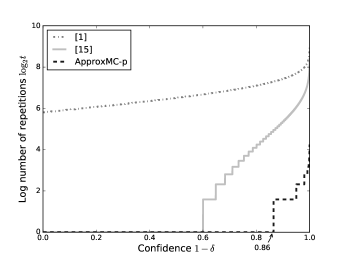
The upper curve visualizes $t(1-\delta)=\lceil 35\cdot\log_{2}(3/\delta)\rceil$ as used in [2]. The middle one is $t(1-\delta)=\min\left(\left\{n\in\mathbb{N}:\delta\geq\sum_{k=\lceil n/2\rceil}^{n}\binom{n}{k}\cdot(2/5)^{k}\cdot(1-(2/5))^{n-k}\right\}\right)$ as used in the master thesis [16] connected to the publication [2]. The lower curve is the function in Algorithm 3, Line 3 for $r=3$.

Figure 1: Comparison of required number of repetitions $t$ of Core (logarithmic scale) for desired level of confidence $1-\delta$

In comparison to the original ApproxMC [2], following differences are of note:

Elimination of $\bot$. The original versions of Core and Main potentially returned an error value $\bot$ instead of an estimation. This distinction has not been exploited to achieve smaller values for $\mathit{pivot}$ and $t$ and hence has been dropped here for more compact and more understandable proofs.

Test $|\varphi|\leq\mathit{pivot}$ hoisted out of the inner loop. The result of this test does not change when repeating Core, so it has been moved to Main.

Smaller values for $\mathit{pivot}$. We have performed a more exact estimation of the needed value of $\mathit{pivot}$. Our value of $\mathit{pivot}$, as defined in Algorithm 3, Line 2, is at least $15\%$ smaller than in [2] (cf. Table 1).

Increased base confidence (fewer repetitions). The number of repetitions needed for the demanded confidence has been substantially reduced (Table 2 and Figure 1). The reasons for this are twofold. First, in [2], the Chernoff-Hoeffding inequality is missing the floor operator, unnecessarily reducing the base confidence. Second, in [2], the “successful” termination of the loop in Core and the tolerable quality of the achieved estimation are treated as independent events and their probabilities multiplied. We show in Theorem 2.12 that the latter actually entails the former.

Table 1: Sample values for $\mathit{pivot}$ depending on the tolerance

	tolerance ($\epsilon$)
	0.75	0.5	0.25	0.1	0.05	0.03	0.01	0.005	0.001
$\mathit{pivot}$ in [2]	54	90	248	1198	4364	11662	100912	399660	9912124
$\mathit{pivot}$ now	27	51	168	922	3517	9584	84575	336622	8382049

Table 2: Sample values for $t$ depending on the confidence

	confidence ($1-\delta$)
	0.5	0.6	0.7	0.8	0.9	0.95	0.99	0.999	0.9999
$t$ in [2]	91	102	117	137	172	207	289	405	521
$t$ in [16]	1	1	7	17	41	67	133	235	339
$t$ now	1	1	1	1	3	3	7	13	19

3.2 Implementation

We have implemented ApproxMC-p and make our implementation available. Algorithms Core and Main are implemented in Python, while different implementations of Bounded#SAT can be plugged in. As the source of random bits we use Python’s Mersenne Twister PRNG, seeded with entropy obtained from /dev/urandom (Linux kernel PRNG seeded from hardware noise). We have chosen a pseudo-random number generator instead of a true randomness source (e.g., the HotBits service used in [2]) for reasons of reproducibility and ease of benchmarking. By reusing the random seed it is possible to reproduce results and also benchmark different implementations of Bounded#SAT.

Our principal Bounded#SAT implementation is based on Cryptominisat5 [22], which is a recent successor to Cryptominisat4. Cryptominisat5 has built-in support for model enumeration and efficient XOR-SAT solving by using the Gauss-Jordan elimination as an inprocessing step. We modified the tool to support projection by shortening the blocking clauses used for model enumeration.

It is also possible to use other model enumerators such as sharpCDCL or CLASP [6]. However, these tools are not designed with native support for XORs. As such they cannot directly parse XOR-CNF inputs, an issue that we work around by translating XORs into CNF using Tseitin encoding. The tools do not employ Gauss-Jordan elimination either, which makes them not competitive against Cryptominisat5 in our scenario. In the future, it would be interesting to benchmark these enumerators combined with Gauss-Jordan elimination as a preprocessing step, though they would still lack inprocessing in the style of Cryptominisat5.

3.3 Experiments

An off-the-shelf program verification system together with projection and counting components is sufficient to implement an analysis quantifying information flow in programs (QIF) [11]. The measured number of reachable final program states corresponds to the min-entropy leakage resp. min-capacity of the program [21] and can be used as a measure of confidentiality or integrity. For generating verification conditions we are using the bounded model checker CBMC [14], for projection and counting ApproxMC-p. The experiments were performed on a machine with an Intel Core i7 860 2.80GHz CPU (same machine as in [12]). ApproxMC-p was configured with the default tolerance $\epsilon=0.5$ and confidence $1-\delta=0.86$.

Synthetic QIF benchmarks.

In [17], the authors describe a series of QIF benchmarks, which have become quite popular since then. As was already noted in [12], the majority of the benchmarks are too easy in the meantime. We use two scaled-up benchmark instances, which could not be solved in [12] without help of a dedicated SAT preprocessor [15].

In both benchmarks, the size of the projection scope $|\Delta|=32$, and $|{\left.\kern-1.2pt\varphi\vphantom{\big{|}}\right|_{\Delta}}|=2^{32}$. The first benchmark, sum-three-32, contains 639 variables and 1708 clauses. The average run time of ApproxMC-p was 1.2s. The average run time for bin-search-32 (4473 variables, 14011 clauses) was 5.2s.

Quantifying information flow in PRNGs.

In [4], we present an information flow analysis aimed at detecting a certain class of errors in pseudo-random number generators (PRNGs). An error is present when the information flow from a seed of $M$ bytes to an $N$-byte chunk of output is not maximal. In [4] we detect such deviations from maximality but do not obtain a quantitative measure of the flow. While quantifying the flows needed for practical application in the domain (at least 20 bytes) is still not feasible, this scenario provides a scalable benchmark.

Here, we are quantifying the flow through the OpenSSL PRNG with cryptographic primitives replaced by idealizations. For $M=N=10$, the 59-megabyte formula contains 590 thousands variables and 2.5 millions clauses. ApproxMC-p counts all $2^{80}$ models in 10.5 minutes (631.7s on average), which is beyond the capabilities of any other counting tool known to us. The largest flow we could measure in this benchmark was at 15 bytes (measured in a single experiment over the course of 47 hours), while reaching the count of 14 bytes in the same experiment took only roughly 32 minutes.

4 Conclusion

The experiments show that ApproxMC-p can effectively and efficiently estimate model counts of projected formulas that are not amenable to other counting tools. At the same time, ApproxMC-p, like any tool, has its own particular pragmatical properties, which need to be carefully considered when choosing a tool for an application.

First, ApproxMC-p offers no approximation advantage for formulas with few models. For instance, at tolerance level $\epsilon=0.1$, formulas with fewer than 922 models are counted exactly (cf. Table 1). On the other hand, there is no penalty for these formulas either, as ApproxMC-p then simply behaves as Bounded#SAT, which offers the best pragmatics for this class of formulas. For formulas with model counts larger but still comparable with $\mathit{pivot}$, ApproxMC-p will perform more SAT queries than Bounded#SAT, due to search for the proper number of buckets and experiment repetition at confidence values over $0.86$ (base confidence). We also note that performance of ApproxMC-p does not increase by lowering the confidence under $0.86$.

Concerning enumeration performance, Cryptominisat5 is currently the best overall implementation of Bounded#SAT due to its built-in support for XORs. Yet, beside Gauss-Jordan elimination, there are various other factors influencing performance (if to a lesser degree): non-XOR solver performance, enumeration algorithm, solver preprocessor, etc. To better understand the individual contributions of these factors, much more benchmarking and investigation is needed.

Finally, ApproxMC-p, in general, does not make larger formulas amenable to counting, merely formulas with more models. For QIF analyses, this means that ApproxMC-p is attractive for quantifying confidentiality in systems with large secrets, as acceptable information leakage is coupled to the secret size. Alternatively, ApproxMC-p can be used for quantifying integrity and related properties.

Acknowledgment.

This work was in part supported by the German National Science Foundation (DFG) under the priority programme 1496 “Reliably Secure Software Systems – RS3.” The authors would like to thank Mate Soos for very helpful feedback concerning Cryptominisat.

Appendix A Detailed Proofs

Proof of Corollary 2.7.

$$\Pr[|\Gamma-\mu|\geq\epsilon\cdot\mu]\leq e^{\lfloor-r/2\rfloor} \iff P[|\Gamma-\mu|\leq\epsilon\cdot\mu]\geq 1-e^{\lfloor-r/2\rfloor}$$

$$\iff P[\Gamma\in[\mu-\epsilon\cdot\mu,\mu+\epsilon\cdot\mu]]\geq 1-e^{\lfloor-r/2\rfloor}$$

$$\iff\Pr[(1-\epsilon)\cdot\mu\leq\Gamma\leq(1+\epsilon)\cdot\mu]\geq 1-e^{\lfloor-r/2\rfloor}$$

∎

Proof of Lemma 2.9.

1. (Measurable) function application preserves independence.

2. We will prove that strong $r$-universality implies strict $r-1$-universality. The claim of the theorem corresponds to strict $1$-universality.

   Assuming, there are at least $r$ distinct keys in $K$ and that $B=\{w_{1},\ldots,w_{|B|}\}$:

   $$\Pr_{h\in H}\big{[}\bigwedge_{i=1}^{r-1}h(k_{i})=v_{i}\big{]}= h(k_{r})$$ existence of

   $$\Pr_{h\in H}\big{[}\bigwedge_{i=1}^{r-1}h(k_{i})=v_{i}\wedge\bigvee_{j=1}^{|B|}h(k_{r})=w_{j}\big{]}=$$ distributivity

   $$\Pr_{h\in H}\big{[}\bigvee_{j=1}^{|B|}(\bigwedge_{i=1}^{r-1}h(k_{i})=v_{i}\wedge h(k_{r})=w_{j})\big{]}=$$ orthogonal disjuncts

   $$\sum_{j=1}^{|B|}\Pr_{h\in H}\big{[}\bigwedge_{i=1}^{r-1}h(k_{i})=v_{i}\wedge h(k_{r})=w_{j}\big{]}= r$$ strong -universality

   $$|B|\cdot\left(\frac{1}{|B|}\right)^{r}=\left(\frac{1}{|B|}\right)^{r-1}\enspace.$$

∎

Proof of Lemma 2.13.

$$1+\log_{2}\left((1+\epsilon)\cdot\frac{|\varphi|}{\mathit{pivot}}\right)\leq\log_{2}\left(\frac{|\varphi|\cdot\epsilon^{2}}{r\cdot\sqrt[3]{e}}\right)$$

$$\iff \log_{2}(2)+\log_{2}\left((1+\epsilon)\cdot\frac{|\varphi|}{pivot}\right)\leq\log_{2}\left(\frac{|\varphi|\cdot\epsilon^{2}}{r\cdot\sqrt[3]{e}}\right)$$

$$\iff \log_{2}\left(2\cdot(1+\epsilon)\cdot\frac{|\varphi|}{pivot}\right)\leq\log_{2}\left(\frac{|\varphi|\cdot\epsilon^{2}}{r\cdot\sqrt[3]{e}}\right)$$

$$\iff 2\cdot(1+\epsilon)\cdot\frac{|\varphi|}{pivot}\leq\frac{|\varphi|\cdot\epsilon^{2}}{r\cdot\sqrt[3]{e}}$$

$$\iff \left\lceil\frac{2\cdot r\cdot(1+\epsilon)\cdot\sqrt[3]{e}}{\epsilon^{2}}\right\rceil\leq pivot$$

∎

Proof of Lemma 2.14.

Lemma 2.14 a and c are widely known and b is trivial with a. Therefore only d will be proved.

Firstly, because for all $k\in\{\lceil n/2\rceil,\ldots,n\}$ it is true that $\binom{n}{k}\leqslant 2^{n}$ it holds:

$$\sum_{k=\lceil n/2\rceil}^{n}\binom{n}{k}\cdot p^{k}\cdot(1-p)^{n-k} =(1-p)^{n}\cdot\left(\sum_{k=\lceil n/2\rceil}^{n}\binom{n}{k}\cdot\left(\frac{p}{1-p}\right)^{k}\right)$$

$$\leq(1-p)^{n}\cdot 2^{n}\cdot\left(\sum_{k=\lceil n/2\rceil}^{n}\cdot\left(\frac{p}{1-p}\right)^{k}\right)$$ (8)

Secondly, due to the restriction of $p$ to be in $[0,1/2]$ the value $(p/(1-p))^{\lceil n/2\rceil}$ is smaller than or equal to $(p/(1-p))^{n/2}$. Hence it applies:

$$\sum_{k=t}^{n}\left(\frac{p}{1-p}\right)^{k}\leq\frac{1-p}{1-2\cdot p}\cdot\left(\sqrt{\frac{p}{1-p}}\right)^{n}$$ (9)

The following estimation shows that:

$$\sum_{k=\lceil n/2\rceil}^{n}\left(\frac{p}{1-p}\right)^{k} =\sum_{k=0}^{n}\left(\frac{p}{1-p}\right)^{k}-\left(\sum_{k=0}^{\lceil n/2\rceil-1}\left(\frac{p}{1-p}\right)^{k}\right)$$

$$\overset{\text{\ref{lemma:coin_tosses_3}}}{=}\frac{1-\left(\frac{p}{1-p}\right)^{n+1}}{1-\frac{p}{1-p}}-\frac{1-\left(\frac{p}{1-p}\right)^{\lceil n/2\rceil}}{1-\frac{p}{1-p}}$$

$$=\frac{1-p}{1-2\cdot p}\cdot\left(\left(\frac{p}{1-p}\right)^{\lceil n/2\rceil}-\left(\frac{p}{1-p}\right)^{n+1}\right)$$

$$\leq\frac{1-p}{1-2\cdot p}\cdot\left(\frac{p}{1-p}\right)^{\lceil n/2\rceil}$$

$$=\frac{1-p}{1-2\cdot p}\cdot\left(\sqrt{\frac{p}{1-p}}\right)^{n}$$

If Equation 9 is inserted into Equation A you get:

$$\frac{1-p}{1-2\cdot p}\cdot\underbrace{2^{n}\cdot(1-p)^{n}\cdot\left(\sqrt{\frac{p}{1-p}}\right)^{n}}_{=\left(\sqrt{4\cdot p\cdot(1-p)}\right)^{n}}$$

∎

References

- [1]
- [2] Supratik Chakraborty, Kuldeep S. Meel & Moshe Y. Vardi (2013): A Scalable Approximate Model Counter. In Christian Schulte, editor: Principles and Practice of Constraint Programming - 19th International Conference, CP 2013, Uppsala, Sweden, September 16-20, 2013. Proceedings, Lecture Notes in Computer Science 8124, Springer, pp. 200–216, 10.1007/978-3-642-40627-0_18.
- [3] Supratik Chakraborty, Kuldeep S. Meel & Moshe Y. Vardi (2014): Balancing Scalability and Uniformity in SAT Witness Generator. In: Proceedings of the 51st Annual Design Automation Conference, DAC ’14, ACM, pp. 60:1–60:6, 10.1145/2593069.2593097.
- [4] Felix Dörre & Vladimir Klebanov (2016): Practical Detection of Entropy Loss in Pseudo-Random Number Generators. In: Proceedings, ACM Conference on Computer and Communications Security (CCS). To appear.
- [5] Stefano Ermon, Carla P Gomes & Bart Selman (2012): Uniform solution sampling using a constraint solver as an oracle. arXiv preprint arXiv:1210.4861.
- [6] Martin Gebser, Benjamin Kaufmann, André Neumann & Torsten Schaub (2007): Clasp: A Conflict-Driven Answer Set Solver. In Chitta Baral, Gerhard Brewka & John Schlipf, editors: Logic Programming and Nonmonotonic Reasoning, Lecture Notes in Computer Science 4483, Springer Berlin Heidelberg, pp. 260–265, 10.1007/978-3-540-72200-7_23.
- [7] Vibhav Gogate & Rina Dechter (2011): SampleSearch: Importance sampling in presence of determinism. Artificial Intelligence 175(2), pp. 694–729, 10.1016/j.artint.2010.10.009.
- [8] Carla P. Gomes, Ashish Sabharwal & Bart Selman (2006): Model Counting: A New Strategy for Obtaining Good Bounds. In: Proceedings of the 21st National Conference on Artificial Intelligence - Volume 1, AAAI’06, AAAI Press, pp. 54–61.
- [9] Carla P. Gomes, Ashish Sabharwal & Bart Selman (2006): Near-Uniform Sampling of Combinatorial Spaces Using XOR Constraints. In Bernhard Schölkopf, John C. Platt & Thomas Hoffman, editors: Advances in Neural Information Processing Systems 19, Proceedings of the Twentieth Annual Conference on Neural Information Processing Systems, Vancouver, British Columbia, Canada, December 4-7, 2006, MIT Press, pp. 481–488.
- [10] Richard M Karp, Michael Luby & Neal Madras (1989): Monte-Carlo approximation algorithms for enumeration problems. Journal of algorithms 10(3), pp. 429–448, 10.1016/0196-6774(89)90038-2.
- [11] Vladimir Klebanov (2014): Precise Quantitative Information Flow Analysis – A Symbolic Approach. Theoretical Computer Science 538(0), pp. 124–139, 10.1016/j.tcs.2014.04.022.
- [12] Vladimir Klebanov, Norbert Manthey & Christian Muise (2013): SAT-based Analysis and Quantification of Information Flow in Programs. In: Proceedings, International Conference on Quantitative Evaluation of Systems, LNCS 8054, Springer, pp. 156–171, 10.1007/978-3-642-40196-1_16.
- [13] Lukas Kroc, Ashish Sabharwal & Bart Selman (2008): Leveraging Belief Propagation, Backtrack Search, and Statistics for Model Counting. In: Proceedings of the 5th International Conference on Integration of AI and OR Techniques in Constraint Programming for Combinatorial Optimization Problems, CPAIOR’08, Springer-Verlag, pp. 127–141, 10.1007/978-3-540-68155-7_12.
- [14] Daniel Kroening & Michael Tautschnig (2014): CBMC – C Bounded Model Checker. In Erika brah m & Klaus Havelund, editors: Tools and Algorithms for the Construction and Analysis of Systems, Lecture Notes in Computer Science 8413, Springer Berlin Heidelberg, pp. 389–391, 10.1007/978-3-642-54862-8_26.
- [15] Norbert Manthey (2012): Coprocessor 2.0: a flexible CNF simplifier. In: Proceedings of the 15th International Conference on Theory and Applications of Satisfiability Testing, Springer-Verlag, Berlin, Heidelberg, pp. 436–441, 10.1007/978-3-642-31612-8_34.
- [16] Kuldeep S Meel (2014): Sampling Techniques for Boolean Satisfiability. arXiv preprint arXiv:1404.6682.
- [17] Ziyuan Meng & Geoffrey Smith (2011): Calculating bounds on information leakage using two-bit patterns. In: Proceedings of the ACM SIGPLAN 6th Workshop on Programming Languages and Analysis for Security, ACM, p. 1, 10.1145/2166956.2166957.
- [18] Christian Muise, Sheila A. McIlraith, J. Christopher Beck & Eric I. Hsu (2012): Dsharp: fast d-DNNF compilation with sharpSAT. In: Proceedings, Canadian AI’12, Springer-Verlag, Berlin, Heidelberg, pp. 356–361, 10.1007/978-3-642-30353-1_36.
- [19] Reuven Rubinstein (2013): Stochastic enumeration method for counting NP-hard problems. Methodology and Computing in Applied Probability 15(2), pp. 249–291, 10.1007/s11009-011-9242-y.
- [20] Jeanette P Schmidt, Alan Siegel & Aravind Srinivasan (1995): Chernoff-Hoeffding bounds for applications with limited independence. SIAM Journal on Discrete Mathematics 8(2), pp. 223–250, 10.1137/S089548019223872X.
- [21] Geoffrey Smith (2015): Recent Developments in Quantitative Information Flow (Invited Tutorial). In: Proceedings of the 2015 30th Annual ACM/IEEE Symposium on Logic in Computer Science (LICS), LICS ’15, IEEE Computer Society, pp. 23–31, 10.1109/LICS.2015.13.
- [22] Mate Soos, Karsten Nohl & Claude Castelluccia (2009): Extending SAT Solvers to Cryptographic Problems. In: Proceedings of the 12th International Conference on Theory and Applications of Satisfiability Testing, SAT ’09, Springer-Verlag, Berlin, Heidelberg, pp. 244–257, 10.1007/978-3-642-02777-2_24.
- [23] Marc Thurley (2006): sharpSAT: Counting Models with Advanced Component Caching and Implicit BCP. In: Proceedings of the 9th International Conference on Theory and Applications of Satisfiability Testing, SAT’06, Springer-Verlag, Berlin, Heidelberg, pp. 424–429, 10.1007/11814948_38.
- [24] Mark N. Wegman & J. Lawrence Carter (1981): New hash functions and their use in authentication and set equality. Journal of Computer and System Sciences 22(3), pp. 265 – 279, 10.1016/0022-0000(81)90033-7.
- [25] Wei Wei & Bart Selman (2005): A New Approach to Model Counting. In: Proceedings of the 8th International Conference on Theory and Applications of Satisfiability Testing, SAT’05, Springer-Verlag, Berlin, Heidelberg, pp. 324–339, 10.1007/11499107_24.