Quantum radiation produced by the entanglement of quantum fields

Abstract

We investigate the quantum radiation produced by an Unruh-De Witt detector in a uniformly accelerating motion coupled to the vacuum fluctuations. Quantum radiation is nonvanishing, which is consistent with the previous calculation by Lin and Hu [Phys. Rev. D 73, 124018 (2006)]. We infer that this quantum radiation from the Unruh-De Witt detector is generated by the nonlocal correlation of the Minkowski vacuum state, which has its origin in the entanglement of the state between the left and the right Rindler wedges.

I Introduction

An accelerated observer sees the Minkowski vacuum state as a thermally excited state, which is characterized by the Unruh temperature $T_{U}=a/2\pi$, where $a$ is the acceleration. By the equivalence principle Unruh ; UnruhWald , the Unruh effect can be understood in analogy with the Hawking radiation, which predicts the thermal radiation from black holes. Since both relativity and quantum mechanics simultaneously play important roles in these effects, detection of the Unruh effect will have a big impact on the research of fundamental physics (cf. SokolovTernov ).

Signals of the Unruh effect will be tiny since the Unruh temperature is very low, $T_{U}=4\times 10^{-20}(a/9.8[{\rm m/s^{2}}])$K for typical values of acceleration. Chen and Tajima pointed out a nice idea of testing the Unruh effect using intense laser’s electric field for accelerating an electron, which has inspired many following works ChenTajima ; Schutzhold ; Schutzhold2 ; ELI . However, subsequent investigations demonstrated that naively expected quantum radiations from thermal random motions induced by the Unruh effect almost cancel out due to the interference effect IYZ ; OYZ15 ; OYZ16 . These works also showed the cancellation is not complete and some quantum radiation remains, though its physical origin is not well understood.

In order to clarify the possible signature of the Unruh effect in the quantum radiation, we revisit the problem of the quantum radiation emanated from an Unruh-De Witt detector in the uniformly accelerating motion Raine ; Raval ; LH ; Lin ; IYZ2013 . We find nonvanishing quantum radiation, which is consistent with the previous calculation by Lin and Hu LH . We point out that this quantum radiation is related to the nonlocal correlation nature of the Minkowski vacuum state, which has its origin in the entanglement of the state between the left and the right Rindler wedges.

This paper is organized as follows. In section 2, we review the model of the Unruh-De Witt detector coupled to a massless scalar field. In section 3, we derive the nonvanishing quantum radiation form the the Unruh-De Witt detector. In section 4, we discuss about the origin of the nonvanishing quantum radiation. Section 5 is devoted to summary and conclusions. In the appendix, a mathematical formula to describe the quantum radiation flux is presented.

II Unruh-De Witt detector model

We consider the model consisting of a massless scalar field $\phi$ and a harmonic oscillator $Q$, which we call an Unruh-De Witt detector, described by the action,

$$S[Q,\phi;z]=\frac{m}{2}\int d\tau\left(\dot{Q}^{2}(\tau)-\Omega_{0}^{2}Q^{2}(\tau)\right)$$

$$~{}~{}+{1\over 2}\int d^{4}x\partial^{\mu}\phi(x)\partial_{\mu}\phi(x)$$

$$~{}~{}+\lambda\int d^{4}xd\tau Q(\tau)\phi(x)\delta^{(4)}_{D}(x-z(\tau)),$$ (2.1)

where $m$ and $\Omega_{0}$ are the mass and the angular frequency of the harmonic oscillator, respectively, $\lambda$ is the coupling constant, and $\delta^{(4)}_{D}(x-y)$ is the 4-dimensional Dirac delta function. The world line trajectory of the detector is specified by $x^{\mu}=z^{\mu}(\tau)$, where $\tau$ is the proper time of the detector. We consider the trajectory in a uniformly accelerated motion $z^{\mu}(\tau)=a^{-1}\left(\sinh{a\tau},\cosh{a\tau},0,0\right)$. Equations of motion for $Q(\tau)$ and $\phi(x)$ are given by

$$\ddot{Q}(\tau)+\Omega_{0}^{2}Q(\tau)={\lambda\over m}\phi(z(\tau)),$$ (2.2)

$$\partial^{2}\phi(x)=\lambda\int d\tau Q(\tau)\delta^{(4)}_{D}(x-z(\tau)).$$ (2.3)

The solution of the scalar field is written as a sum of the homogeneous solution $\phi_{\rm h}(x)$ and the inhomogeneous solution $\phi_{\rm inh}(x)$, i.e., $\phi(x)=\phi_{\rm h}(x)+\phi_{\rm inh}(x)$. $\phi_{\rm inh}(x)$ is given by $\phi_{\rm inh}(x)=\lambda\int d\tau Q(\tau)G_{R}(x-z(\tau))$, where $G_{R}(x-y)$ is the retarded Green function of the massless scalar field. Using the regularized retarded Green function, (2.2) becomes

$$\ddot{Q}(\tau)+2\gamma\dot{Q}(\tau)+\Omega^{2}Q(\tau)={\lambda\over m}\phi_{\rm h}(z(\tau)),$$ (2.4)

where we introduced $\gamma=\lambda^{2}/8\pi m$ and the renormalized frequency $\Omega$ (see Ref. LH ).

Using the Fourier transformations,

$$Q(\tau)={1\over 2\pi}\int_{-\infty}^{\infty}d\omega e^{-i\omega\tau}\tilde{Q}(\omega),$$ (2.5)

$$\phi_{\rm h}(z(\tau))={1\over 2\pi}\int_{-\infty}^{\infty}d\omega e^{-i\omega\tau}\varphi(\omega),$$ (2.6)

Eq. (2.4) is solved as $\tilde{Q}(\omega)=\lambda h(\omega)\varphi(\omega)$ with $h(\omega)={1/(-m\omega^{2}+m\Omega^{2}-i2m{\omega\gamma})}.$ By inserting this solution (2.5) into the expression of $\phi_{\rm inh}(x)$, we have

$$\phi_{\rm inh}(x)=\lambda^{2}\int d\tau\int{d\omega\over 2\pi}e^{-i\omega\tau}h(\omega)G_{R}(x-z(\tau))\varphi(\omega).$$

(2.7)

In the present paper, we consider the case $\Omega<\gamma$, in which the poles of $h(\omega)$ are located at $\omega=-i\Omega_{\pm}$ where we defined $\Omega_{\rm\pm}=\gamma\pm\sqrt{\gamma^{2}-\Omega^{2}}$.

It is useful to verify that the detector is in thermal equilibrium at the Unruh temperature. The expectation value of energy of the harmonic oscillator is computed using the solution (2.5) with $h(\omega)$ as

$$\langle E\rangle={m\over 2}\left(\langle\dot{Q}^{2}(\tau)\rangle+\Omega^{2}\langle Q^{2}(\tau)\rangle\right)={a\over 2\pi}$$ (2.8)

under the condition $\Omega_{\pm}\ll a$. Thus the law of the equipartition of energy with the Unruh temperature is satisfied as a consequence of the Unruh effect.

III Radiation from the Unruh-De Witt detector

Since the detector is in the thermal equilibrium, one may expect that the would-be radiation due to the thermal fluctuation is cancelled by the quantum interference effect. Actually that is the case for the $1+1$ dimensional case. The $1+3$ dimensional case has a similar structure of the cancellation, and we misconcluded in Ref. IYZ2013 that the quantum radiation from the uniformly accelerating Unruh-De Witt detector is completely cancelled. But more careful calculations show that some part of the radiation remains. Our new conclusion is consistent with that in Ref.LH , in which they also demonstrated nonvanishing radiation flux. In the present paper, we give an analytic expression for the radiation and some interpretation of the origin of the radiation.

In order to calculate the radiation from the detector, we evaluate the energy momentum tensor of the quantum field. First, we consider the two point function IYZ ; IYZ2013 . Since the total radiation rate can be estimated from the flux in the F-region in Fig. 1, we focus on the two point function,

$$\langle\phi(x)\phi(y)\rangle-\langle\phi_{\rm h}(x)\phi_{\rm h}(y)\rangle$$ (3.1)

$$= \langle\phi_{\rm inh}(x)\phi_{\rm h}(y)\rangle+\langle\phi_{\rm h}(x)\phi_{\rm inh}(y)\rangle+\langle\phi_{\rm inh}(x)\phi_{\rm inh}(y)\rangle$$

$$= {-i\lambda^{2}\over(4\pi)^{2}\rho_{0}(x)\rho_{0}(y)}\int_{-\infty}^{+\infty}{d\omega\over 2\pi}{e^{\pi\omega/a}\over e^{2\pi\omega/a}-1}$$

$$\bigr{[}h(\omega)e^{-i\omega(\tau_{-}^{x}-\tau_{+}^{y})}-h(-\omega)e^{-i\omega(\tau_{+}^{x}-\tau_{-}^{y})}\bigl{]},$$

for $x,y\in$ F-region, where we defined $\rho_{0}(x)=a\sqrt{(-x_{\mu}x^{\mu}+1/a^{2})^{2}/4+((x^{0})^{2}-(x^{1})^{2})/a^{2}}$. Here, $\tau_{-}^{x}$ is defined as the proper time at which the detector’s trajectory intersects with the past lightcone of a spacetime point $x$. On the other hand, $\tau_{+}^{x}$ is the proper time at which the hypothetical detector’s trajectory in the L-region intersects with the past lightcone of $x$ for $x\in$ F-region. $\tau_{\pm}^{y}$ is defined in the same way. (See figure 1).

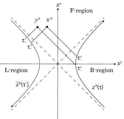
Figure 1: The R-region is defined by $x^{1}>|x^{0}|$, the L-region is $-x^{1}>|x^{0}|$, and the F-region is $x^{0}>|x^{1}|$. The hyperbolic curve $z^{\mu}(\tau)$ in the R-region is the trajectory of a uniformly accelerating Unruh-De Witt detector, while the hyperbolic curve in the L-region $\widetilde{z}^{\mu}(\tau)$ is the hypothetical trajectory obtained by an analytic continuation of the trajectory in the R-region. $\tau_{-}^{x}$ is defined by the proper time at which the detector’s trajectory intersects with the past lightcone of $x^{\mu}$. On the other hand, for a point $y^{\mu}$ in the F-region, $\tau_{+}^{y}$ is defined by the proper time that the hypothetical detector’s trajectory in the L-region intersects with the past lightcone of $y^{\mu}$.

After performing the integration of (3.1), the two point function symmetrized with respect to $x$ and $y$ is expressed as

$$[\langle\phi(x)\phi(y)\rangle-\langle\phi_{\rm h}(x)\phi_{\rm h}(y)\rangle]_{S}$$

$$=-{i\lambda^{2}\over(4\pi)^{2}\rho_{0}(x)\rho_{0}(y)}{1\over 2m}\left(I(x,y)+I(y,x)\right),$$ (3.2)

where $I(x,y)$ is defined by

$$I(x,y)=$$

$$-i\theta(\tau_{-}^{y}-\tau_{+}^{x})\biggl{[}{1\over\Omega_{+}\Omega_{-}}{a\over 2\pi}+{e^{-\Omega_{-}(\tau_{-}^{y}-\tau_{+}^{x})}\over\Omega_{-}-\Omega_{+}}{1\over\sin\pi\Omega_{-}/a}$$

$$+{e^{-\Omega_{+}(\tau_{-}^{y}-\tau_{+}^{x})}\over\Omega_{+}-\Omega_{-}}{1\over\sin\pi\Omega_{+}/a}+\sum_{n=1}^{\infty}{(-1)^{n}e^{-na(\tau_{-}^{y}-\tau_{+}^{x})}\over(\Omega_{-}-na)(\Omega_{+}-na)}{a\over\pi}\biggr{]}$$

$$+i\theta(\tau_{+}^{x}-\tau_{-}^{y})\biggl{[}{1\over\Omega_{+}\Omega_{-}}{a\over 2\pi}+\sum_{n=1}^{\infty}{(-1)^{n}e^{na(\tau_{-}^{y}-\tau_{+}^{x})}\over(\Omega_{-}+na)(\Omega_{+}+na)}{a\over\pi}\biggr{]}.$$

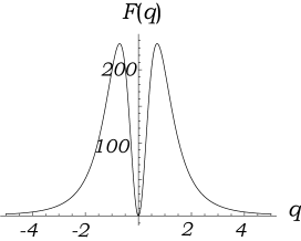
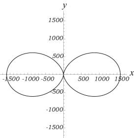
Figure 2: Upper panel: ${\cal F}(q)$ as function of $q$, where we chose $\Omega/a=0.01$ and $\gamma/a=1$. Lower panel: Angular distribution of the flux $\sin^{-4}{\theta}{\cal F}(q(\tau_{-},\theta))$ at $\tau_{-}=0$, where we chose the same parameters as those of the upper panel. The coordinates $x$ and $y$ are $x^{1}$ and $\sqrt{(x^{2})^{2}+(x^{3})^{2}}$, respectively.

We are now interested in the energy flux $f=-\sum_{i}T_{0i}n^{i}$, where $T_{0i}$ is the time and space component of the energy momentum tensor and $n^{i}$ is the unit vector $n^{i}=x^{i}/r$, which is computed from the two point function,

$$T_{0i}=\lim_{y\rightarrow x}{\partial\over\partial x^{0}}{\partial\over\partial y^{i}}[\langle\phi(x)\phi(y)\rangle-\langle\phi_{\rm h}(x)\phi_{\rm h}(y)\rangle]_{S}.$$ (3.4)

Using the expression (3.2), we can derive an exact expression for the energy flux (cf. OYZ15 ; OYZ16 ). The exact formula (see Appendix) is very complicated, but in the case $\Omega<\gamma$, it can be very well approximated by the following formula,

$$f={a\lambda^{2}\over(4\pi)^{2}mr^{2}\sin^{4}\theta}{\cal F}(q,\Omega_{+}/a,\Omega_{-}/a),$$ (3.5)

where we defined

$${\cal F}(q,\Omega_{+}/a,\Omega_{-}/a)={q^{2}\over(1+q^{2})^{3}}\biggl{[}-\theta(q)\biggl{\{}{a^{2}\over\Omega_{+}\Omega_{-}}{1\over 2\pi}$$

$$+{a\over{\Omega_{-}}-{\Omega_{+}}}\biggl{(}{{-q+\sqrt{1+q^{2}}}\over{q+\sqrt{1+q^{2}}}}\biggr{)}^{\Omega_{-}/a}{1\over\sin\pi\Omega_{-}/a}\biggr{\}}$$

$$+\theta(-q)\biggl{\{}{a^{2}\over\Omega_{+}\Omega_{-}}{1\over 2\pi}\biggr{\}}\biggr{]}$$ (3.6)

and $q=a\left(t-r-{1/(2a^{2}r)}\right)/\sin\theta.$ The upper panel of Fig. 2 exemplifies the function ${\cal F}(q)$ adopting ${\gamma/a}=1$ and ${\Omega/a}=0.01$. The lower panel of Fig. 2 shows the corresponding angular plot of ${\cal F}(q)/\sin^{4}\theta$ at $\tau_{-}=0$ (see also Refs.OYZ15 ; OYZ16 )

The order of the energy radiation rate is roughly estimated as

$${dE\over dt}=\lim_{r\rightarrow\infty}r^{2}\int d\Omega_{(2)}f\sim{a\lambda^{2}\over 4\pi m}{\cal F}\sim{a\lambda^{2}\over 4\pi m}{a^{2}\over 2\pi\Omega^{2}}.$$ (3.7)

This result is consistent with that of Ref.LH , though their result assumes the weak coupling case $\Omega>\gamma$.

IV Interpretation of the Result

We will now point out that the physical origin of the remaining radiation is related to the quantum entanglement of the vacuum between the left and the right Rindler wedges. Using the properties of the retarded Green function

$$\int d\tau G_{R}(x,z(\tau))J(\tau)={J(\tau_{-}^{x})\over 4\pi\rho_{0}(x)},$$ (4.1)

for a function $J(\tau)$, the two point function (3.1) with $x,y\in$ F-region can be rewritten as

$$\langle\phi(x)\phi(y)\rangle-\langle\phi_{\rm h}(x)\phi_{\rm h}(y)\rangle=-i\lambda^{2}\int\frac{d\omega}{2\pi}{e^{\pi\omega/a}\over e^{2\pi\omega/a}-1}$$

$$~{}~{}\int d\tau\int d\tau^{\prime}e^{-i\omega(\tau-\tau^{\prime})}\biggl{[}G_{R}(x,z(\tau))G_{R}(y,\widetilde{z}(\tau^{\prime}))h(\omega)$$

$$~{}~{}-G_{R}(x,\widetilde{z}(\tau))G_{R}(y,z(\tau^{\prime}))h(-\omega)\biggr{]},$$ (4.2)

where $\widetilde{z}(\tau)$ denotes the hypothetical trajectory in the L region. On the other hand, the correlation of the inhomogeneous term, which is cancelled by the interference term, is given by IYZ ; IYZ2013 ,

$$\langle\phi_{\rm inh}(x)\phi_{\rm inh}(y)\rangle=-i\lambda^{2}\int\frac{d\omega}{2\pi}{e^{2\pi\omega/a}\over e^{2\pi\omega/a}-1}$$

$$~{}~{}\int d\tau\int d\tau^{\prime}e^{-i\omega(\tau-\tau^{\prime})}\biggl{[}G_{R}(x,z(\tau))G_{R}(y,z(\tau^{\prime}))h(\omega)$$

$$~{}~{}-G_{R}(x,z(\tau))G_{R}(y,z(\tau^{\prime}))h(-\omega)\biggr{]}.$$ (4.3)

These two correlations, (4.2) and (4.3), look very similar but are different in the following two points, and both of them indicate that the remaining two point function (4.2) reflects the nonlocal correlation of the Minkowski vacuum state for the following two reasons.

First, Eq. (4.3) expresses the two point correlation of the field produced by the detector in the R-region, which is described by the retarded Green function connecting two points on the trajectory $z^{\mu}(\tau)$ in the $R$-region (see Fig. 1). It is due to the fact that the inhomogeneous part of the field $\phi_{\rm inh}$ is determined by the quantum fluctuations on the real trajectory (2.7). On the other hand, Eq. (4.2) is obtained by replacing one of the two points on the trajectory $z^{\mu}(\tau)$ in the R-region with $\widetilde{z}^{\mu}(\tau)$ in the L-region. This reflects the fact that the correlation function $\langle\phi_{\rm h}(x)\phi_{\rm inh}(y)\rangle$ contains the correlation between the R and the L regions. Namely, the entanglement of the quantum fluctuations between the R-region and the L-region will be responsible for the remaining radiation in Eq. (4.2).

The second difference between (4.2) and (4.3) is the numerical factors of $e^{\pi\omega/a}$ and $e^{2\pi\omega/a}$. It is also a signature of the entanglement of fields between the R-region and the L-region. By introducing the Rindler coordinates in the R-region and the L-region, the quantum field operator is constructed in each region, respectively, and we may write the field operator as UnruhWald ; Higuchi ,

$$\psi=\psi_{\rm R}\theta(x^{1}-x^{0})+\psi_{\rm L}\theta(x^{0}-x^{1}),$$ (4.4)

with

$$\psi_{\rm R}=\sum_{j}\left(u_{j}(x_{\tiny{\rm R}})\hat{a}_{j}+u_{j}^{*}(x_{\tiny{\rm R}})\hat{a}_{j}^{\dagger}\right),$$ (4.5)

$$\psi_{\rm L}=\sum_{j}\left(v_{j}(x_{\tiny{\rm L}})\hat{b}_{j}+v_{j}^{*}(x_{\tiny{\rm L}})\hat{b}_{j}^{\dagger}\right),$$ (4.6)

where $\psi_{\rm R}$ and $\psi_{\rm L}$ are the quantum field operators, $u_{j}(x_{\tiny{\rm R}})$ and $v_{j}(x_{\tiny{\rm L}})$ are the mode functions, and $\hat{a}_{j}(\hat{a}_{j}^{\dagger})$ and $\hat{b}_{j}(\hat{b}_{j}^{\dagger})$ are the annihilation (creation) operators of Rindler particles in the R-region and the L-region, respectively. Accordingly the Rindler vacuum states, $|0,{\rm R}\rangle$ and $|0,{\rm L}\rangle$, are defined by the annihilation operator, $\hat{a}_{j}$ or $\hat{b}_{j}$. The Minkowski vacuum state $|0,{\rm M}\rangle$ is expressed by the superposed state of the excited states of the Rindler vacuum UnruhWald ; Higuchi ,

$$|0,{\rm M}\rangle=\prod_{j}\biggl{[}N_{j}\sum_{n_{j}=0}^{\infty}e^{-\pi n_{j}\omega_{j}/a}|n_{j},{\rm R}\rangle\otimes|n_{j},{\rm L}\rangle\biggr{]},$$

where $|n_{j},{\rm R}\rangle$ and $|n_{j},{\rm L}\rangle$ are the $n$th excited states of the mode $j$ for the Rindler particles in the R-region and in the L-region, respectively. $\omega_{j}$ is the energy of a Rindler particle of the mode $j$, and $N_{j}=\sqrt{1-e^{-2\pi\omega_{j}/a}}$. This expression describes the entanglement of the Minkowski vacuum state, as the entangled states of the R-region and the L-region.

Let us consider the field operator of the form (4.5) but with $u_{j}(x_{R})$ being replaced by another function $\tilde{u}_{j}(x_{R})$, which we define $\widetilde{\psi}(x_{\rm R})=\sum_{j}\left(\tilde{u}_{j}(x_{\tiny{\rm R}})\hat{a}_{j}+\tilde{u}_{j}^{*}(x_{\tiny{\rm R}})\hat{a}_{j}^{\dagger}\right)$. By choosing points, $x$ and $y$ in the R-region and in the L-region, respectively, the correlation function $\langle 0,{\rm M}|\widetilde{\psi}(x)\psi(y)|0,{\rm M}\rangle$ can be obtained as

$$\langle 0,{\rm M}|\widetilde{\psi}(x_{R})\psi(y_{L})|0,{\rm M}\rangle=\sum_{j}(\tilde{u}_{j}(x_{\tiny{\rm R}})v_{j}(y_{\tiny{\rm L}})$$

$$~{}+\tilde{u}_{j}^{*}(x_{\tiny{\rm R}})v_{j}^{*}(y_{\tiny{\rm L}})){e^{\pi\omega_{j}/a}\over e^{2\pi\omega_{j}/a}-1}.$$ (4.8)

Here the factor $e^{\pi\omega/a}/(e^{2\pi\omega/a}-1)$ appears when the two points are chosen in the R-region and the L-region. This comes from the relations $\langle 0,{\rm M}|\hat{b}_{j}\hat{a}_{j}|0,{\rm M}\rangle=\langle 0,{\rm M}|\hat{a}_{j}^{\dagger}\hat{b}_{j}^{\dagger}|0,{\rm M}\rangle\propto e^{\pi\omega/a}/(e^{2\pi\omega/a}-1)$, and the same factor appears in (4.2).

On the other hand, when two points $x$ and $y$ are in the R-region, the two point correlation function becomes

$$\langle 0,{\rm M}|\widetilde{\psi}(x_{R})\psi(y_{R})|0,{\rm M}\rangle=\sum_{j}\bigl{(}\tilde{u}_{j}(x_{\tiny{\rm R}}){u}_{j}^{*}(y_{\tiny{\rm R}}){e^{2\pi\omega_{j}/a}\over e^{2\pi\omega_{j}/a}-1}$$

$$~{}+\tilde{u}_{j}^{*}(x_{\tiny{\rm R}}){u}_{j}(y_{\tiny{\rm R}}){1\over e^{2\pi\omega_{j}/a}-1}\bigr{)}.$$ (4.9)

Note that a different numerical factor $e^{2\pi\omega/a}$ appears in the numerator. This comes from the relations $\langle 0,{\rm M}|\hat{a}_{j}\hat{a}_{j}^{\dagger}|0,{\rm M}\rangle\propto e^{2\pi\omega/a}/(e^{2\pi\omega/a}-1)$ and $\langle 0,{\rm M}|\hat{a}_{j}^{\dagger}\hat{a}_{j}|0,{\rm M}\rangle\propto 1/(e^{2\pi\omega/a}-1)$, and this is nothing but the numerical factor in (4.3). By changing the integration variable from $\omega$ to $\omega^{\prime}=-\omega$, the function $1/(e^{2\pi\omega/a}-1)$ is expressed as $e^{2\pi\omega^{\prime}/a}/(1-e^{2\pi\omega^{\prime}/a})$ and becomes the same numerical factor.

Thus, the above arguments show that the difference in the numerical factors of $e^{\pi\omega/a}$ and $e^{2\pi\omega/a}$ can be interpreted as an indication of the entanglement of the Minkowski vacuum between the right Rindler wedge and the left Rindler wedge as Eq. (IV).

V Summary and Conclusions

In summary the influence of the detector in the quantum vacuum is generated in the R-region, which is described by $\phi_{\rm inh}(x)$, and propagates into the F-region. However, the system cannot be closed within the R-region. As we showed, the remaining energy flux in the F-region, which can be calculated from the two point functions there, depends on the interference between $\phi_{\rm inh}(x)$ and $\phi_{h}(x)$ in the F-region. Due to the causality, properties of the quantum field $\phi_{\rm h}(x)$ in the F-region are influenced by the properties of the quantum states not only in the R-region but also in the L-region. Since the Minkowski vacuum is entangled between these two regions, the correlation function of $\phi_{\rm inh}(x)$ and $\phi_{h}(x)$ contains the information of the entanglement of the Minkowski vacuum. If there was no entanglement, the energy flux would be completely cancelled out and vanish. Thus, we can conclude that the remaining radiation is a consequence of the nonlocal correlation (or the entanglement) of the Minkowski vacuum between the R and L regions, and it may be called the quantum radiation.

Detectability of the quantum radiation is an interesting issue, and in order to discuss it, we first need to extend the present calculation to more realistic systems. It is also necessary to satisfy the condition that thermalization time (or the relaxation time) $\tau_{R}={8\pi m/\lambda^{2}}=\gamma^{-1}$ LH , with which the system becomes in an equilibrium phase, must be shorter than the time during which a uniform acceleration is maintained. We hope to discuss these issues in future publications.

Appendix

In the appendix we just show the result of the exact formula for the energy flux (3.5) with

$${\cal F}(q,\widetilde{\Omega}_{+},\widetilde{\Omega}_{-})={q^{2}\over(1+q^{2})^{3}}\biggl{[}-\theta(q)\biggl{\{}{1\over\widetilde{\Omega}_{+}}{1\over\widetilde{\Omega}_{-}}{1\over 2\pi}+{\xi^{\widetilde{\Omega}_{-}}(q)\over{\widetilde{\Omega}_{-}}-{\widetilde{\Omega}_{+}}}{1\over\sin\pi\widetilde{\Omega}_{-}}+{\xi^{\widetilde{\Omega}_{+}}(q)\over{\widetilde{\Omega}_{+}}-{\widetilde{\Omega}_{-}}}{1\over\sin\pi\widetilde{\Omega}_{+}}$$

$$+{\xi(q)\over{\widetilde{\Omega}_{-}}-{\widetilde{\Omega}_{+}}}\biggl{(}{1\over{1-{\widetilde{\Omega}_{+}}}}{}_{2}F_{1}(1,1-\widetilde{\Omega}_{+},2-\widetilde{\Omega}_{+};-\xi(q))-{1\over{1-\widetilde{\Omega}_{-}}}{}_{2}F_{1}(1,1-\widetilde{\Omega}_{-},2-\widetilde{\Omega}_{-};-\xi(q))\biggr{)}{1\over\pi}\biggr{\}}$$

$$+\theta(-q)\biggl{\{}{1\over\widetilde{\Omega}_{+}}{1\over\widetilde{\Omega}_{-}}{1\over 2\pi}+{\xi^{-1}(q)\over\widetilde{\Omega}_{-}-\widetilde{\Omega}_{+}}\biggl{(}{1\over{1+\widetilde{\Omega}_{-}}}{}_{2}F_{1}(1,1+\widetilde{\Omega}_{-},2+\widetilde{\Omega}_{-};-\xi^{-1}(q))$$

$$-{1\over{1+\widetilde{\Omega}_{+}}}{}_{2}F_{1}(1,1+\widetilde{\Omega}_{+},2+\widetilde{\Omega}_{+};-\xi^{-1}(q))\biggr{)}{1\over\pi}\biggr{\}}\biggr{]}-2{q\over(1+q^{2})^{5/2}}\biggl{[}-\theta(q)\biggl{\{}-{{\widetilde{\Omega}_{-}}\over{\widetilde{\Omega}_{-}-\widetilde{\Omega}_{+}}}{\xi^{\widetilde{\Omega}_{-}}(q)\over\sin\pi\widetilde{\Omega}_{-}}$$

$$-{\widetilde{\Omega}_{+}\over\widetilde{\Omega}_{+}-\widetilde{\Omega}_{-}}{\xi^{\widetilde{\Omega}_{+}}(q)\over\sin\pi\widetilde{\Omega}_{+}}+{\xi(q)\over{\widetilde{\Omega}_{-}-\widetilde{\Omega}_{+}}}\biggl{(}-{1\over{1-\widetilde{\Omega}_{+}}}{}_{2}F_{1}(2,1-\widetilde{\Omega}_{+},2-\widetilde{\Omega}_{+};-\xi(q))+{1\over{1-\widetilde{\Omega}_{-}}}$$

$${}_{2}F_{1}(2,1-\widetilde{\Omega}_{-},2-\widetilde{\Omega}_{-};-\xi(q))\biggr{)}{1\over\pi}\biggr{\}}+\theta(-q)\biggl{\{}{\xi^{-1}(q)\over{\widetilde{\Omega}_{-}-\widetilde{\Omega}_{+}}}\biggl{(}-{1\over{1+\widetilde{\Omega}_{+}}}{}_{2}F_{1}(2,1+\widetilde{\Omega}_{+},2+\widetilde{\Omega}_{+};-\xi^{-1}(q))$$

$$+{1\over{1+\widetilde{\Omega}_{-}}}{}_{2}F_{1}(2,1+\widetilde{\Omega}_{-},2+\widetilde{\Omega}_{-};-\xi^{-1}(q))\biggr{)}{1\over\pi}\biggr{\}}\biggr{]}-{1\over(1+q^{2})^{2}}\biggl{[}-\theta(q)\biggl{\{}-{\widetilde{\Omega}_{-}^{2}\over\widetilde{\Omega}_{-}-\widetilde{\Omega}_{+}}{\xi^{\widetilde{\Omega}_{-}}(q)\over\sin\pi\widetilde{\Omega}_{-}}-{\widetilde{\Omega}_{+}^{2}\over\widetilde{\Omega}_{+}-\widetilde{\Omega}_{-}}$$

$${\xi^{\widetilde{\Omega}_{+}}(q)\over\sin\pi\widetilde{\Omega}_{+}}+{1\over\widetilde{\Omega}_{-}-\widetilde{\Omega}_{+}}\biggl{(}{\xi(q)\over 1-\widetilde{\Omega}_{-}}{}_{2}F_{1}(2,1-\widetilde{\Omega}_{-},2-\widetilde{\Omega}_{-};-\xi(q))-{\xi(q)\over 1-\widetilde{\Omega}_{+}}{}_{2}F_{1}(2,1-\widetilde{\Omega}_{+},2-\widetilde{\Omega}_{+};-\xi(q))$$

$$-{2\xi^{2}(q)\over 2-\widetilde{\Omega}_{-}}{}_{2}F_{1}(3,2-\widetilde{\Omega}_{-},3-\widetilde{\Omega}_{-};-\xi(q))+{2\xi^{2}(q)\over 2-\widetilde{\Omega}_{+}}{}_{2}F_{1}(3,2-\widetilde{\Omega}_{+},3-\widetilde{\Omega}_{+};-\xi(q))\biggr{)}{1\over\pi}\biggr{\}}+\theta(-q)\biggl{\{}$$

$${1\over\widetilde{\Omega}_{-}-\widetilde{\Omega}_{+}}\biggl{(}-{\xi^{-1}(q)\over 1+\widetilde{\Omega}_{-}}{}_{2}F_{1}(2,1+\widetilde{\Omega}_{-},2+\widetilde{\Omega}_{-};-\xi^{-1}(q))+{\xi^{-1}(q)\over 1+\widetilde{\Omega}_{+}}{}_{2}F_{1}(2,1+\widetilde{\Omega}_{+},2+\widetilde{\Omega}_{+};-\xi^{-1}(q)$$

$$+{2\xi^{-2}(q)\over 2+\widetilde{\Omega}_{-}}{}_{2}F_{1}(3,2+\widetilde{\Omega}_{-},3+\widetilde{\Omega}_{-};-\xi^{-1}(q))-{2\xi^{-2}(q)\over 2+\widetilde{\Omega}_{+}}{}_{2}F_{1}(3,2+\widetilde{\Omega}_{+},3+\widetilde{\Omega}_{+};-\xi^{-1}(q))\biggr{)}{1\over\pi}\biggr{\}}\biggr{]},$$ (5.1)

where we defined $\xi(q)=({-q+\sqrt{1+q^{2}})/(q+\sqrt{1+q^{2}}})$, $\widetilde{\Omega}_{+}=\Omega_{+}/a$ and $\widetilde{\Omega}_{-}=\Omega_{-}/a$ . This complicated formula is well approximated by Eq. (3.6) in the case $\Omega<\gamma$.