Fast Bayesian Non-Negative Matrix Factorisation and Tri-Factorisation

Abstract

We present a fast variational Bayesian algorithm for performing non-negative matrix factorisation and tri-factorisation. We show that our approach achieves faster convergence per iteration and timestep (wall-clock) than Gibbs sampling and non-probabilistic approaches, and do not require additional samples to estimate the posterior. We show that in particular for matrix tri-factorisation convergence is difficult, but our variational Bayesian approach offers a fast solution, allowing the tri-factorisation approach to be used more effectively.

1 Introduction

Non-negative matrix factorisation methods Lee and Seung (1999) have been used extensively in recent years to decompose matrices into latent factors, helping us reveal hidden structure and predict missing values. In particular we decompose a given matrix into two smaller matrices so that their product approximates the original one. The non-negativity constraint makes the resulting matrices easier to interpret, and is often inherent to the problem – such as in image processing or bioinformatics (Lee and Seung (1999); Wang et al. (2013)). Some approaches approximate a maximum likelihood (ML) or maximum a posteriori (MAP) solution that minimises the difference between the observed matrix and the decomposition of this matrix. This gives a single point estimate, which can lead to overfitting more easily and neglects uncertainty. Instead, we may wish to find a full distribution over the matrices using a Bayesian approach, where we define prior distributions over the matrices and then compute their posterior after observing the actual data.

Schmidt et al. (2009) presented a Bayesian model for non-negative matrix factorisation that uses Gibbs sampling to obtain draws of these posteriors, with exponential priors to enforce non-negativity. Markov chain Monte Carlo (MCMC) methods like Gibbs sampling rely on a sampling procedure to eventually converge to draws of the desired distribution – in this case the posterior of the matrices. This means that we need to inspect the values of the draws to determine when our method has converged (burn-in), and then take additional draws to estimate the posteriors.

We present a variational Bayesian approach to non-negative matrix factorisation, where instead of relying on random draws we obtain a deterministic convergence to a solution. We do this by introducing a new distribution that is easier to compute, and optimise it to be as similar to the true posterior as possible. We show that our approach gives faster convergence rates per iteration and timestep (wall-clock) than current methods, and is less prone to overfitting than the popular non-probabilistic approach of Lee and Seung (2000).

We also consider the problem of non-negative matrix tri-factorisation, first introduced by Ding et al. (2006), where we decompose the observed dataset into three smaller matrices, which again are constrained to be non-negative. Matrix tri-factorisation has been explored extensively in recent years, for example for collaborative filtering (Chen et al. (2009)) and clustering genes and phenotypes (Hwang et al. (2012)). We present a fully Bayesian model for non-negative matrix tri-factorisation, extending the matrix factorisation model to obtain both a Gibbs sampler and a variational Bayesian algorithm for inference. We show that convergence is even harder, and that the variational approach provides significant speedups (roughly four times faster) compared to Gibbs sampling.

2 Non-Negative Matrix Factorisation

We follow the notation used by Schmidt et al. (2009) for non-negative matrix factorisation (NMF), which can be formulated as decomposing a matrix $\boldsymbol{R}\in\mathbb{R}^{I\times J}$ into two latent (unobserved) matrices $\boldsymbol{U}\in\mathbb{R}_{+}^{I\times K}$ and $\boldsymbol{V}\in\mathbb{R}_{+}^{J\times K}$. In other words, solving $\boldsymbol{R}=\boldsymbol{U}\boldsymbol{V}^{T}+\boldsymbol{E}$, where noise is captured by matrix $\boldsymbol{E}\in\mathbb{R}^{I\times J}$. The dataset $\boldsymbol{R}$ need not be complete – the indices of observed entries can be represented by the set $\Omega=\left\{(i,j)\text{ $|$ $R_{ij}$ is observed}\right\}$. These entries can then be predicted by $\boldsymbol{U}\boldsymbol{V}^{T}$.

We take a probabilistic approach to this problem. We express a likelihood function for the observed data, and treat the latent matrices as random variables. As the likelihood we assume each value of $\boldsymbol{R}$ comes from the product of $\boldsymbol{U}$ and $\boldsymbol{V}$, with some Gaussian noise added,

$$R_{ij}\sim\mathcal{N}(R_{ij}|\boldsymbol{U}_{i}\cdot\boldsymbol{V}_{j},\tau^{-1})$$

where $\boldsymbol{U}_{i},\boldsymbol{V}_{j}$ denote the $i$th and $j$th rows of $\boldsymbol{U}$ and $\boldsymbol{V}$, and $\mathcal{N}(x|\mu,\tau)$ is the density of the Gaussian distribution, with precision $\tau$. The full set of parameters for our model is denoted $\boldsymbol{\theta}=\left\{\boldsymbol{U},\boldsymbol{V},\tau\right\}$.

In the Bayesian approach to inference, we want to find the distributions over the parameters $\boldsymbol{\theta}$ after observing the data $D=\{R_{ij}\}_{i,j\in\Omega}$. We can use Bayes’ theorem for this, $p(\boldsymbol{\theta}|D)\propto p(D|\boldsymbol{\theta})p(\boldsymbol{\theta})$. We need priors over the parameters, allowing us to express beliefs for their values – such as constraining $\boldsymbol{U},\boldsymbol{V}$ to be non-negative. We can normally not compute the posterior $p(\boldsymbol{\theta}|D)$ exactly, but some choices of priors allow us to obtain a good approximation. Schmidt et al. choose an exponential prior over $\boldsymbol{U}$ and $\boldsymbol{V}$, so that each element in $U$ and $V$ is assumed to be independently exponentially distributed with rate parameters $\lambda_{ik}^{U},\lambda_{jk}^{V}>0$,

$$U_{ik}\sim\mathcal{E}(U_{ik}|\lambda_{ik}^{U})\quad\quad V_{jk}\sim\mathcal{E}(V_{jk}|\lambda_{jk}^{V})$$

where $\mathcal{E}(x|\lambda)$ is the density of the exponential distribution. For the precision $\tau$ we use a Gamma distribution with shape $\alpha>0$ and rate $\beta>0$.

Schmidt et al. (2009) introduced a Gibbs sampling algorithm for approximating the posterior distribution, which relies on sampling new values for each random variable in turn from the conditional posterior distribution. Details on this method can be found in the supplementary materials (Section 1.1).

Variational Bayes for NMF

Like Gibbs sampling, variational Bayesian inference (VB) is a way to approximate the true posterior $p(\boldsymbol{\theta}|D)$. The idea behind VB is to introduce an approximation $q(\boldsymbol{\theta})$ to the true posterior that is easier to compute, and to make our variational distribution $q(\boldsymbol{\theta})$ as similar to $p(\boldsymbol{\theta}|D)$ as possible (as measured by the KL-divergence). We assume the variational distribution $q(\boldsymbol{\theta})$ factorises completely, so all variables are independent, $q(\boldsymbol{\theta})=\prod_{\theta_{i}\in\boldsymbol{\theta}}q(\theta_{i})$. This is called the mean-field assumption. We assume the same forms of $q(\theta_{i})$ as used in Gibbs sampling,

$$q(\tau)=\mathcal{G}(\tau|\alpha^{*},\beta^{*})\quad\quad\quad q(U_{ik})=\mathcal{TN}(U_{ik}|\mu_{ik}^{U},\tau_{ik}^{U})\quad\quad\quad q(V_{jk})=\mathcal{TN}(V_{jk}|\mu_{jk}^{V},\tau_{jk}^{V})$$

Beal and Ghahramani (2003) showed that the optimal distribution for the $i$th parameter, $q^{*}(\theta_{i})$, can be expressed as follows (for some constant $C$), allowing us to find the optimal updates for the variational parameters

$$\log q^{*}(\theta_{i})=\mathbb{E}_{q(\boldsymbol{\theta}_{-i})}\left[\log p(\boldsymbol{\theta},D)\right]+C.$$

Note that we take the expectation with respect to the distribution $q(\boldsymbol{\theta}_{-i})$ over the parameters but excluding the $i$th one. This gives rise to an iterative algorithm: for each parameter $\theta_{i}$ we update its distribution to that of its optimal variational distribution, and then update the expectation and variance with respect to $q$. This algorithm is guaranteed to maximise the Evidence Lower Bound (ELBO)

$$\mathcal{L}=\mathbb{E}_{q}\left[\log p(\boldsymbol{\theta},D)-\log q(\boldsymbol{\theta})\right],$$

which is equivalent to minimising the KL-divergence. More details and updates for the approximate posterior distribution parameters are given in the supplementary materials (Section 1.2).

3 Non-Negative Matrix Tri-Factorisation

The problem of non-negative matrix tri-factorisation (NMTF) can be formulated similarly to that of non-negative matrix factorisation. We now decompose our dataset $\boldsymbol{R}\in\mathbb{R}^{I\times J}$ into three matrices $\boldsymbol{F}\in\mathbb{R}_{+}^{I\times K}$, $\boldsymbol{S}\in\mathbb{R}_{+}^{K\times L}$, $\boldsymbol{G}\in\mathbb{R}_{+}^{J\times L}$, so that $\boldsymbol{R}=\boldsymbol{F}\boldsymbol{S}\boldsymbol{G}^{T}+\boldsymbol{E}$. We again use a Gaussian likelihood and Exponential priors for the latent matrices.

$$R_{ij}\sim\mathcal{N}(R_{ij}|\boldsymbol{F}_{i}\cdot\boldsymbol{S}\cdot\boldsymbol{G}_{j},\tau^{-1}) \tau\sim\mathcal{G}(\tau|\alpha,\beta)$$

$$F_{ik}\sim\mathcal{E}(F_{ik}|\lambda_{ik}^{F})\quad S_{kl}\sim\mathcal{E}(S_{kl}|\lambda_{kl}^{S})\quad G_{jl}\sim\mathcal{E}(G_{jl}|\lambda_{jl}^{G})$$

A Gibbs sampling algorithm that can be derived similarly to before. Details can be found in the supplementary materials (Section 1.3).

3.1 Variational Bayes for NMTF

Our VB algorithm for tri-factorisation follows the same steps as before, but now has an added complexity due to the term $\mathbb{E}_{q}\left[(R_{ij}-\boldsymbol{F}_{i}\cdot\boldsymbol{S}\cdot\boldsymbol{G}_{j})^{2}\right]$. Before, all covariance terms for $k^{\prime}\neq k$ were zero due to the factorisation in $q$, but we now obtain some additional non-zero covariance terms. This leads to the more complicated variational updates given in the supplementary materials (Section 1.4).

$$\mathbb{E}_{q}\left[(R_{ij}-\boldsymbol{F}_{i}\cdot\boldsymbol{S}\cdot\boldsymbol{G}_{j})^{2}\right]=\left(R_{ij}-\sum_{k=1}^{K}\sum_{l=1}^{L}\widetilde{F_{ik}}\widetilde{S_{kl}}\widetilde{G_{jl}}\right)^{2}+\sum_{k=1}^{K}\sum_{l=1}^{L}\mathrm{Var}_{q}\left[F_{ik}S_{kl}G_{jl}\right]\quad\quad\quad$$

$$\quad\quad\quad+\sum_{k=1}^{K}\sum_{l=1}^{L}\sum_{k^{\prime}\neq k}\mathrm{Cov}\left[F_{ik}S_{kl}G_{jl},F_{ik^{\prime}}S_{k^{\prime}l}G_{jl}\right]+\sum_{k=1}^{K}\sum_{l=1}^{L}\sum_{l^{\prime}\neq l}\mathrm{Cov}\left[F_{ik}S_{kl}G_{jl},F_{ik}S_{kl^{\prime}}G_{jl^{\prime}}\right]$$

4 Experiments

To demonstrate the performances of our proposed methods, we ran several experiments on a toy dataset, as well as several drug sensitivity datasets. For the toy dataset we generated the latent matrices using unit mean exponential distributions, and adding zero mean unit variance Gaussian noise to the resulting product. For the matrix factorisation model we use $I=100,J=80,K=10$, and for the matrix tri-factorisation $I=100,J=80,K=5,L=5$.

We also consider a drug sensitivity dataset, which detail the effectiveness of different drugs on cell lines for cancer and tissue types. The Genomics of Drug Sensitivity in Cancer (GDSC v5.0, Yang et al. (2013)) dataset contains 138 drugs and 622 cell lines, with 81% of entries observed.

We compare our methods against classic algorithms for matrix factorisation and tri-factorisation. Aside from the Gibbs sampler (G-NMF, G-NMTF) and VB algorithms (VB-NMF, VB-NMTF), we consider the non-probabilistic matrix factorisation (NP-NMF) and tri-factorisation (NP-NMTF) methods introduced by Lee and Seung (2000) and Yoo and Choi (2009), respectively. Schmidt et al. (2009) also proposed an Iterated Conditional Modes (ICM-NMF) algorithm for computing an MAP solution, where instead of using draws from the posteriors as updates we set their values to the mode. We also extended this method for matrix tri-factorisation (ICM-NMTF).

4.1 Convergence speed

We tested the convergence speed of the methods on both the toy data, giving the correct values for $K,L$, and on the GDSC drug sensitivity dataset. We track the convergence rate of the error (mean square error) on the training data against the number of iterations taken. This can be found for the toy data in Figures 1(a) (MF) and 1(b) (MTF), and for the GDSC drug sensitivity dataset in Figures 1(c) and 1(d). Below that (Figures 1(e)-1(h)) is the convergence in terms of time (wall-clock), timing each run 10 times and taking the average (using the same random seed).

We see that our VB methods takes the fewest iterations to converge to the best solution. This is especially the case in the tri-factorisation case, where the best solution is much harder to find (note that all methods initially find a worse solution and get stuck on that for a while), and our variational approach converges seven times faster in terms of iterations taken. We note that time wise, the ICM algorithms can be implemented more efficiently than the fully Bayesian approaches, but returns a MAP solution rather than the full posterior. Our VB method still converges four times faster than the other fully Bayesian approach, and twice as fast as the non-probabilistic method.

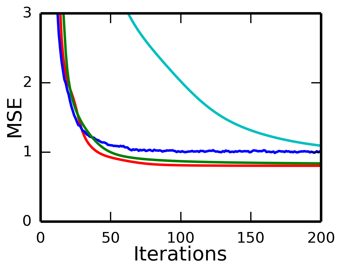
(a) Toy NMF

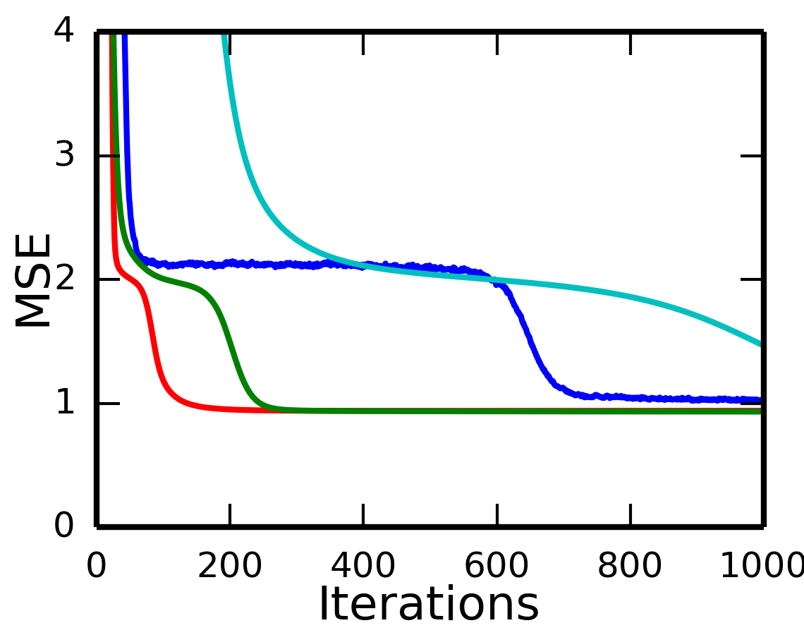
(b) Toy NMTF

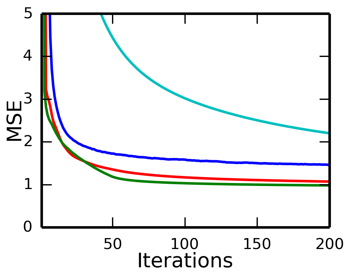
(c) Drug sensitivity NMF

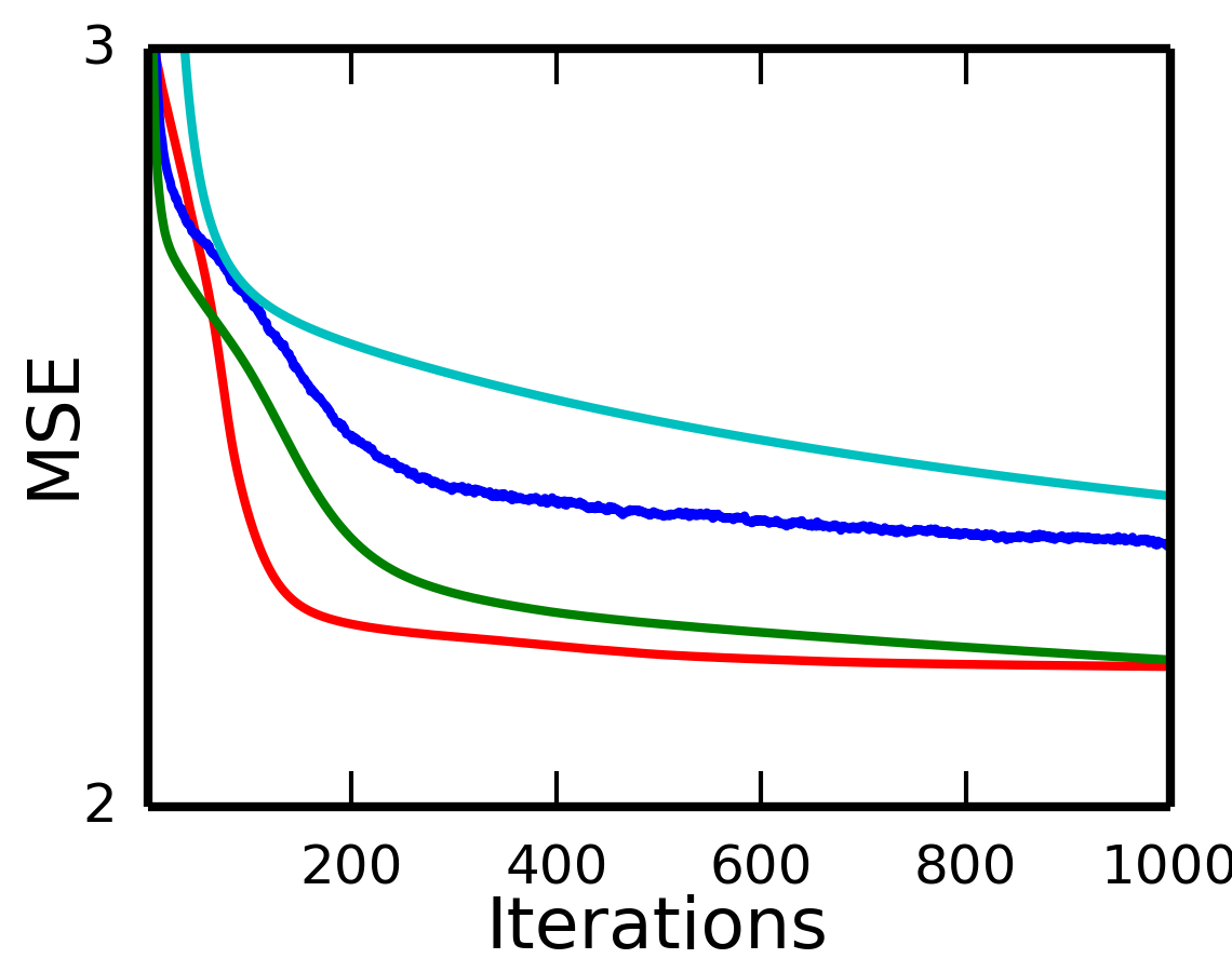
(d) Drug sensitivity NMTF

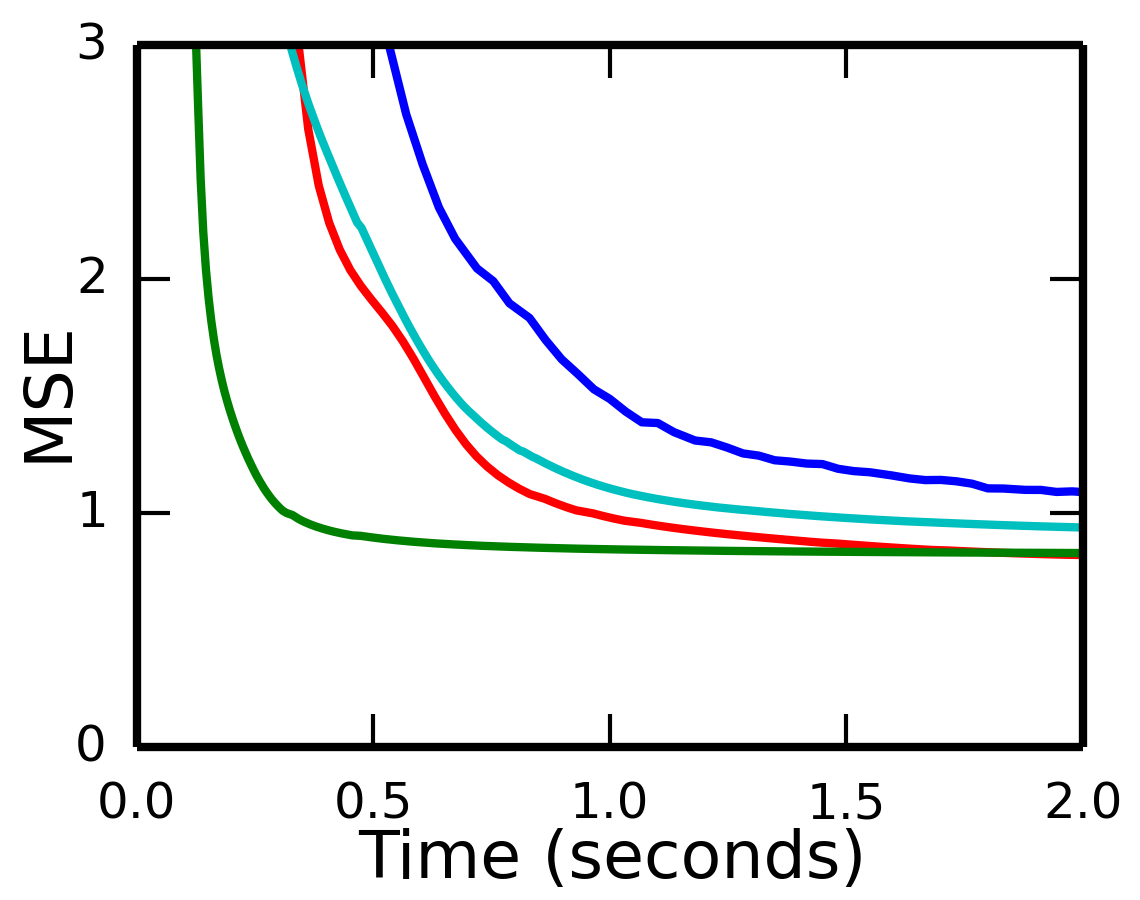
(e) Toy NMF

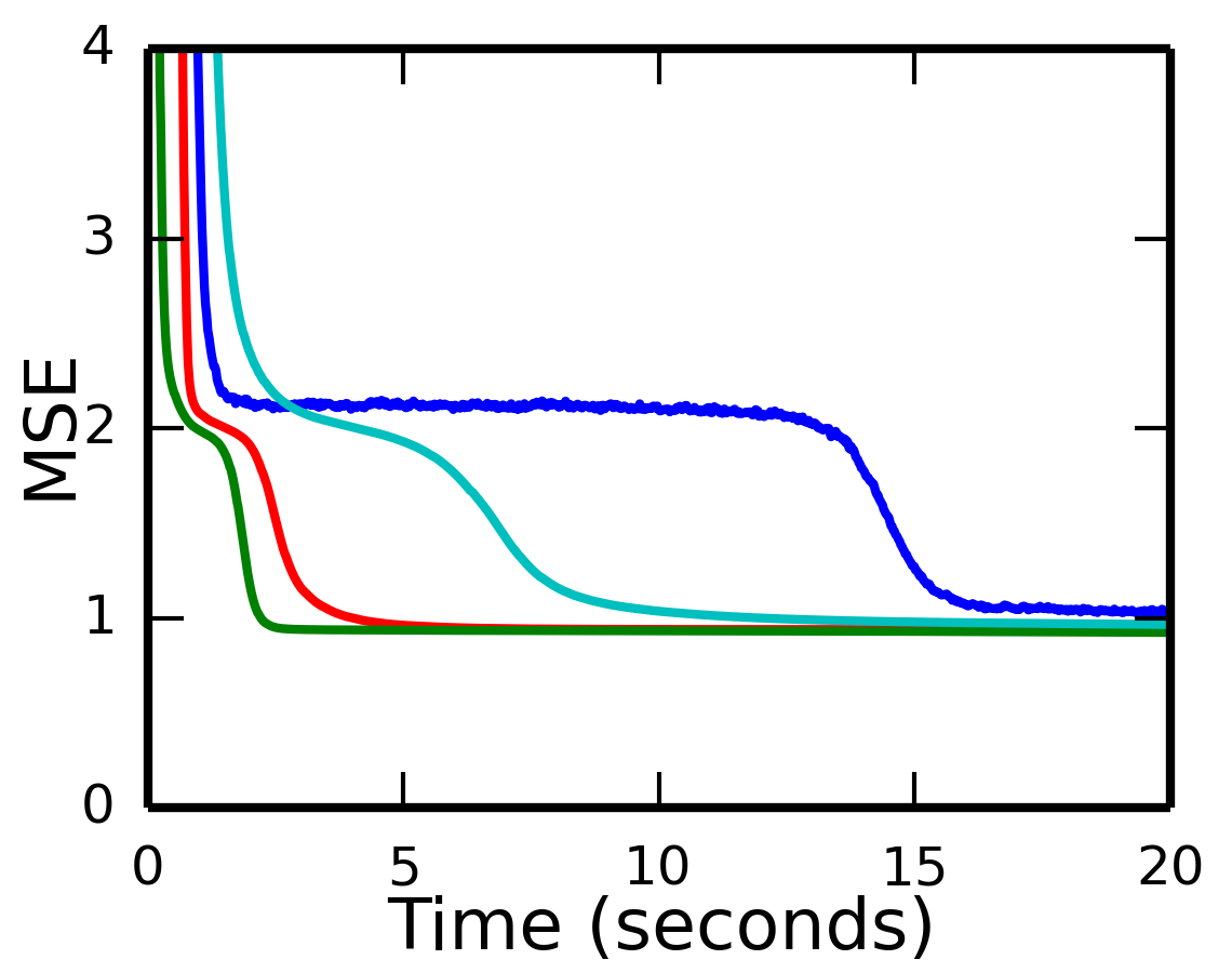
(f) Toy NMTF

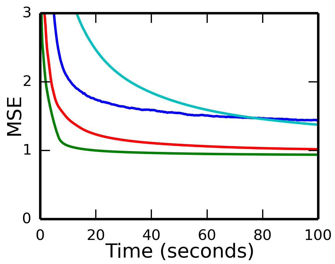
(g) Drug sensitivity NMF

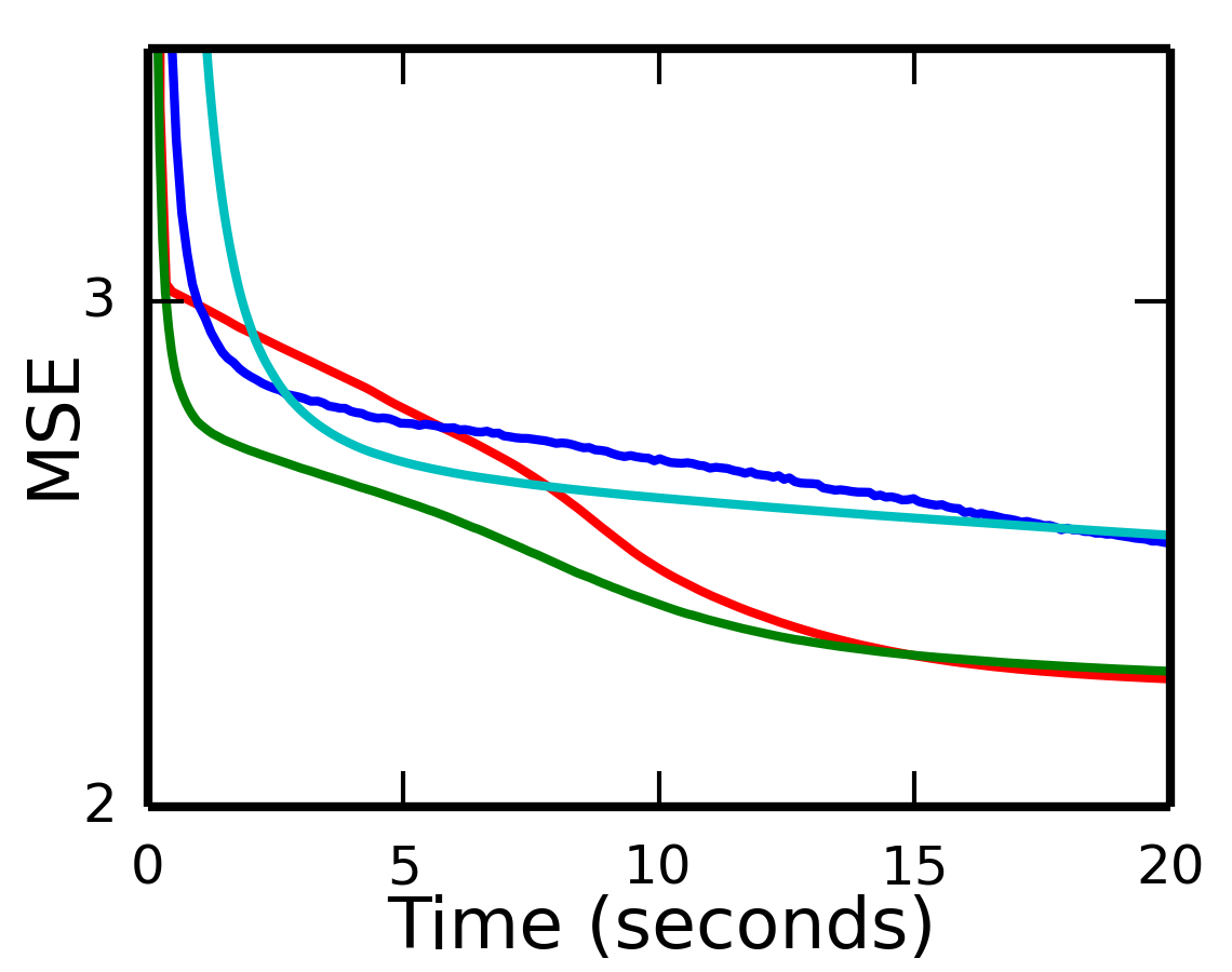
(h) Drug sensitivity NMTF

Figure 1: Convergence of algorithms on the toy and GDSC drug sensitivity datasets, measuring the training data fit (mean square error) across iterations (top row) and time (bottom row).

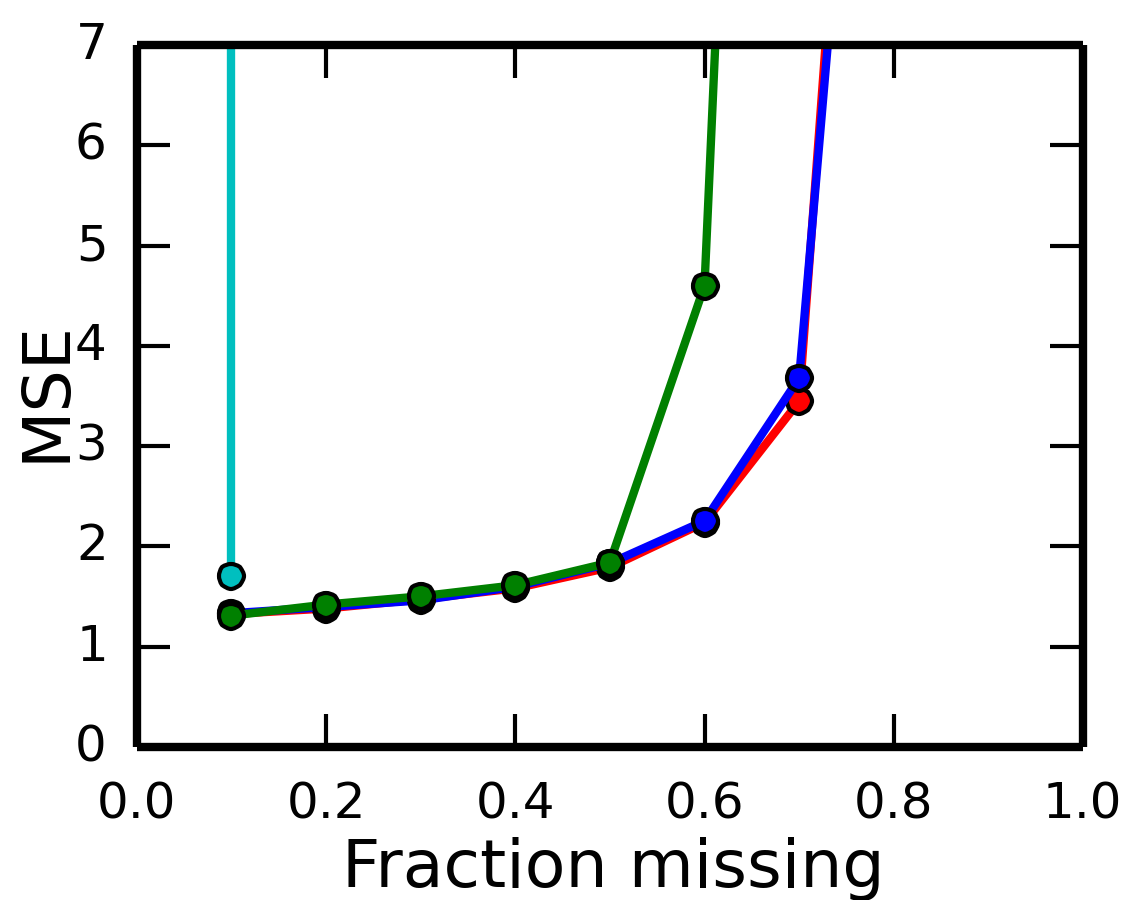
(a) NMF

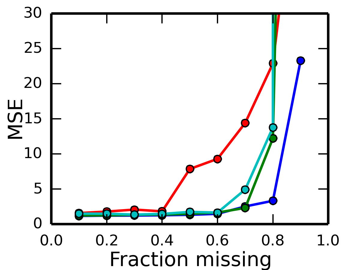
(b) NMTF

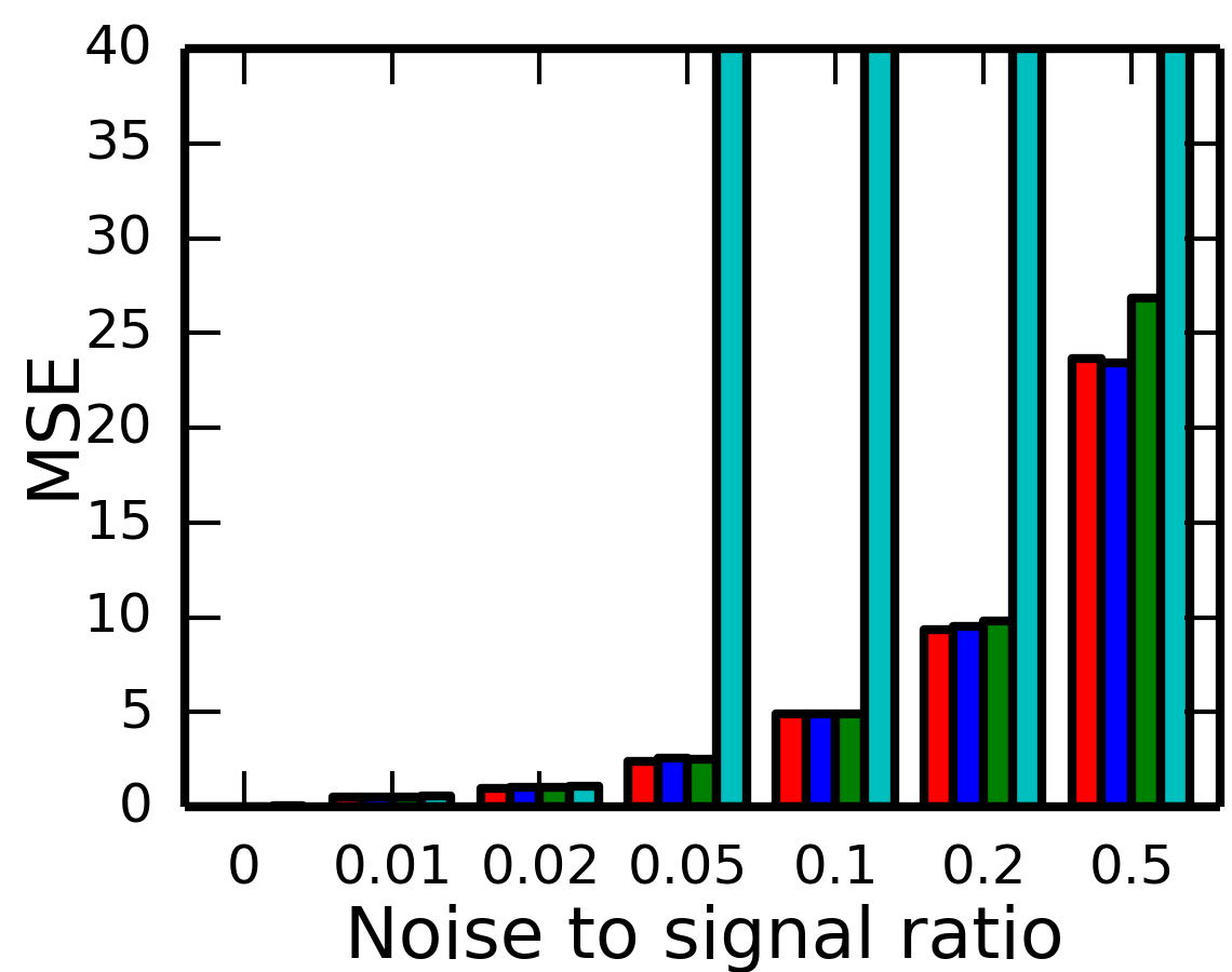
(c) NMF

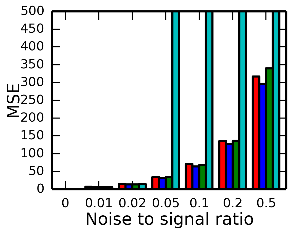
(d) NMTF

Figure 2: Missing values prediction performances (Figures 2(a) and 2(b)) and noise test performances (Figures 2(c) and 2(d)), measured by average predictive performance on test set (mean square error) for different fractions of unknown values and noise-to-signal ratios.

4.2 Other experiments

We conducted several other experiments, such as model selection on toy datasets, and cross-validation on three drug sensitivity datasets. Details and results for all experiments are given in the supplementary materials (Section 3), but here we highlight the results for missing value predictions and noise tests. In Figures 2(a) and 2(b), we measure the ability of the models to predict missing values in a toy dataset as the fraction of missing values increases. Similarly, Figures 2(c) and 2(d) show the predictive performances as the amount of noise in the data increases. The figures show that the Bayesian models are more robust to noise, and perform better on sparse datasets than their non-probabilistic counterparts.

5 Conclusion

We have introduced a fast variational Bayesian algorithm for performing non-negative matrix factorisation and tri-factorisation. We have shown that this method gives us deterministic convergence that is faster than MCMC methods, without requiring additional samples to estimate the posterior distribution. We demonstrate that our variational approach is particularly useful for the tri-factorisation case, where convergence is even harder, and we obtain a four-fold time speedup. These speedups can open up the applicability of the models to larger datasets.

References

- Ammad-ud din et al. (2014) M. Ammad-ud din, E. Georgii, M. Gönen, T. Laitinen, O. Kallioniemi, K. Wennerberg, A. Poso, and S. Kaski. Integrative and personalized QSAR analysis in cancer by kernelized Bayesian matrix factorization. Journal of chemical information and modeling, 54(8):2347–59, Aug. 2014.
- Barretina et al. (2012) J. Barretina, G. Caponigro, N. Stransky, K. Venkatesan, A. A. Margolin, S. Kim, C. J. Wilson, et al. The Cancer Cell Line Encyclopedia enables predictive modelling of anticancer drug sensitivity. Nature, 483(7391):603–7, Mar. 2012.