Real singlet scalar dark matter extension of the Georgi-Machacek model

Abstract

The Georgi-Machacek model extends the Standard Model Higgs sector with the addition of isospin-triplet scalar fields in such a way as to preserve the custodial symmetry. The presence of higher-isospin scalars contributing to electroweak symmetry breaking offers the interesting possibility that the couplings of the 125 GeV Higgs boson to both gluons and vector boson pairs could be larger than those of the Standard Model Higgs boson. Constraining this possibility using measurements of Higgs production and decay at the CERN Large Hadron Collider is notoriously problematic if a new, non-Standard Model decay mode of the 125 GeV Higgs boson is present. We study an implementation of this scenario in which the Georgi-Machacek model is extended by a real singlet scalar dark matter candidate, and require that the singlet scalar account for all the dark matter in the universe. The combination of the observed dark matter relic density and direct detection constraints exclude singlet scalar masses below about 57 GeV. Higgs measurements are not yet precise enough to be very sensitive to $h\rightarrow SS$ in the remaining allowed kinematic region, so that constraints from Higgs measurements are so far the same as in the GM model without a singlet scalar. We also find that, above the Higgs pole, a substantial region of parameter space yielding the correct dark matter relic density can escape the near-future direct detection experiments DEAP and XENON 1T for dark matter masses as low as 120 GeV and even have a direct detection cross section below the neutrino floor for $m_{S}\gtrsim 150$ GeV. This is in contrast to the singlet scalar dark matter extension of the Standard Model, for which these future experiments are expected to exclude dark matter masses above the Higgs pole up to the multi-TeV range.

I Introduction

Since the discovery of a Standard Model (SM)-like 125 GeV Higgs boson at the CERN Large Hadron Collider (LHC) Aad:2012tfa , the determination of the Higgs boson’s couplings to other particles has become a top priority. At the LHC, these couplings are extracted from signal rates in various resonant Higgs production and decay channels, which can be written in the narrow width approximation as

$${\rm Rate}_{ij}=\sigma_{i}\frac{\Gamma_{j}}{\Gamma_{\rm tot}}=\kappa_{i}^{2}\sigma_{i}^{\rm SM}\frac{\kappa_{j}^{2}\Gamma_{j}^{\rm SM}}{\sum_{k}\kappa_{k}^{2}\Gamma_{k}^{\rm SM}+\Gamma_{\rm new}}.$$ (1)

Here $\sigma_{i}$ is the Higgs production cross section in production mode $i$, $\Gamma_{j}$ is the Higgs decay partial width into final state $j$, $\Gamma_{\rm tot}$ is the total width of the Higgs boson, the corresponding quantities in the SM are denoted with a superscript, and $\Gamma_{\rm new}$ represents the partial width of the Higgs boson into any new, non-SM final states. The coupling modification factors $\kappa_{i}$ parameterize the deviations of the Higgs couplings from their SM values LHCHiggsCrossSectionWorkingGroup:2012nn .

The extraction of the Higgs couplings $\kappa_{i}$ from these LHC rate measurements is plagued by a well-known “flat direction” Zeppenfeld:2000td that appears when new decay modes are present. For example, one can imagine a scenario in which all the coupling modification factors have a common value $\kappa_{i}^{2}\equiv\kappa^{2}>1$ and there is a new, unobserved contribution to the Higgs total width, $\Gamma_{\rm new}>0$. In this case the Higgs production and decay rates measurable at the LHC are given by

$${\rm Rate}_{ij}=\frac{\kappa^{4}\sigma_{i}^{\rm SM}\Gamma_{j}^{\rm SM}}{\kappa^{2}\Gamma_{\rm tot}^{\rm SM}+\Gamma_{\rm new}}.$$ (2)

All measured Higgs production and decay rates will be equal to their SM values if

$$\Gamma_{\rm new}=\kappa^{2}(\kappa^{2}-1)\Gamma_{\rm tot}^{\rm SM}\geq 0.$$ (3)

In particular, a simultaneous enhancement $\kappa^{2}>1$ of all the Higgs couplings to SM particles can mask, and be masked by, the presence of new decay modes of the Higgs that are not (yet) directly detected at the LHC.

Our goal in this paper is to study an explicit benchmark model in which this scenario could be realized. We focus on models with extended Higgs sectors. Our first requirement is a model in which the Higgs couplings to $W$ and $Z$ bosons and to fermions can be enhanced relative to those in the SM. To achieve $\kappa_{W},\kappa_{Z}>1$ in an extended Higgs model, we need scalars in isospin representations larger than doublets that carry non-negligible vacuum expectation values (vevs). Only a few such models exist that preserve the $\rho$ parameter at tree level: the Georgi-Machacek (GM) model with isospin triplets Georgi:1985nv ; Chanowitz:1985ug , generalizations of the GM model to higher isospin Galison:1983qg ; Robinett:1985ec ; Logan:1999if ; Chang:2012gn ; Logan:2015xpa , and an extension of the Higgs sector by an isospin septet with appropriately-chosen hypercharge Hisano:2013sn ; Kanemura:2013mc ; Alvarado:2014jva . In this paper we choose the GM model as the simplest extension suitable for our purposes. Its phenomenology has been extensively studied Gunion:1989ci ; Gunion:1990dt ; HHG ; Haber:1999zh ; Aoki:2007ah ; Godfrey:2010qb ; Low:2010jp ; Logan:2010en ; Falkowski:2012vh ; Chang:2012gn ; Chiang:2012cn ; Chiang:2013rua ; Kanemura:2013mc ; Englert:2013zpa ; Killick:2013mya ; Englert:2013wga ; Efrati:2014uta ; Hartling:2014zca ; Chiang:2014hia ; Chiang:2014bia ; Godunov:2014waa ; Hartling:2014aga ; Chiang:2015kka ; Godunov:2015lea . It has also been incorporated into the scalar sectors of little Higgs Chang:2003un ; Chang:2003zn and supersymmetric Cort:2013foa ; Garcia-Pepin:2014yfa models, and an extension with an additional isospin doublet Hedri:2013wea has been considered.

Our second requirement is a new decay mode for the 125 GeV Higgs boson. A particularly attractive prospect is to link Higgs physics to the mystery of dark matter in the universe (for a recent pedagogical review see Ref. Gelmini:2015zpa ) by allowing the Higgs to decay into pairs of dark matter particles. To this end we extend the GM model through the addition of a real isospin-singlet scalar field $S$, upon which we impose a $Z_{2}$ symmetry $S\to-S$. We will require that $S$ accounts for the observed dark matter relic abundance in the universe via the standard thermal freeze-out mechanism. Real singlet scalar extensions of the SM Veltman:1989vw ; Silveira:1985rk ; McDonald:1993ex ; Burgess:2000yq ; McDonald:2001vt ; Barger:2007im ; Goudelis:2009zz ; Gonderinger:2009jp ; He:2009yd ; Profumo:2010kp ; Yaguna:2011qn ; Drozd:2011aa ; Djouadi:2011aa ; Kadastik:2011aa ; Djouadi:2012zc ; Cheung:2012xb ; Damgaard:2013kva ; Cline:2013gha ; Baek:2014jga ; Feng:2014vea ; Campbell:2015fra and of two-Higgs-doublet models He:2008qm ; Grzadkowski:2009iz ; Logan:2010nw ; Boucenna:2011hy ; He:2011gc ; Bai:2012nv ; He:2013suk ; Cai:2013zga ; Wang:2014elb ; Chen:2013jvg ; Drozd:2014yla ; Wang:2014elb ; Campbell:2015fra have been extensively studied in the literature. These models tend to be tightly constrained by the combination of relic density, dark matter direct-detection limits, and limits on the indirect detection of dark matter annihilation byproducts from nearby dwarf galaxies.

We will find that the situation is rather similar in the singlet scalar dark matter extension of the GM model. The two strongest constraints are the requirement of the correct dark matter relic abundance from thermal freeze-out Kolb:1990vq and the direct detection cross section limit from the LUX experiment Akerib:2016vxi . These constraints restrict the allowed range of singlet scalar masses to lie just below the 125 GeV Higgs pole for resonant annihilation (57–62 GeV) or above the $Z$ boson mass. The constraint from 125 GeV Higgs boson invisible decays is currently weaker than that from direct detection. Constraints coming from Higgs properties and signals also significantly constrain this model. They do however allow for some interesting deviations from the Standard Model that the GM model without the singlet does not allow.

One important difference compared to the singlet scalar extension of the SM is the prospect for future dark matter direct detection experiments to probe the model at heavier singlet masses. While an absence of signal at the planned XENON 1T experiment would exclude singlet scalar masses up to 4.5 TeV in the singlet scalar extension of the SM Cline:2013gha , in the singlet scalar extension of the GM model a large swath of parameter space with singlet scalar masses as light as 125 GeV remains beyond the reach of XENON 1T. In fact, there is some allowed parameter space with singlet scalar masses near the 125 GeV Higgs pole for resonant annihilation (60–62 GeV) and some with singlet scalar masses above about 150 GeV which have a direct detection cross section that lies below the neutrino floor. This is mainly due to the contribution of the additional scalars in the GM model to the production of the correct relic density, while not contributing strongly to the direct detection cross section.

This paper is organized as follows. In Sec. II we begin with a description of the singlet scalar extension of the GM model. In Sec. III we extend the theoretical constraints on the GM model to include the singlet scalar extension. In Sec. IV we describe the details of the thermal freezeout and imposing the relic abundance constraints on the model parameters while in Sec. V we describe the numerical scan procedure used to map out the allowed parameter space. In Sec. VI we briefly summarize the direct and indirect search constraints on the additional scalars in the GM model. In Sec. VII we compute the dark matter relic abundance and direct and indirect detection cross sections and display the impact of the observational constraints on the allowed parameter space. In Sec. VIII we consider the constraints from the 125 GeV Higgs boson invisible decays and signal strengths in visible channels. Finally in Sec. IX we summarize our conclusions. Feynman rules for couplings involving the singlet scalar are collected in an appendix.

II The Georgi-Machacek model extended by a real singlet scalar

The scalar sector of the GM model Georgi:1985nv ; Chanowitz:1985ug consists of the usual complex doublet $(\phi^{+},\phi^{0})$ with hypercharge $Y=1$, a real triplet $(\xi^{+},\xi^{0},\xi^{-})$ with $Y=0$, and a complex triplet $(\chi^{++},\chi^{+},\chi^{0})$ with $Y=2$. The doublet is responsible for the fermion masses as in the SM. In order to preserve the custodial SU(2) symmetry and avoid large tree-level contributions to the electroweak $\rho$ parameter, the scalar potential is constructed to preserve a global SU(2)${}_{L}\times$SU(2)_R symmetry, which breaks down to the diagonal subgroup (known as the custodial SU(2) symmetry) upon electroweak symmetry breaking. To make the global SU(2)${}_{L}\times$SU(2)_R symmetry explicit, we write the doublet in the form of a bidoublet $\Phi$ and combine the triplets to form a bitriplet $X$:

$$\Phi=\left(\begin{array}[]{cc}\phi^{0*}&\phi^{+}\\ -\phi^{+*}&\phi^{0}\end{array}\right),\qquad X=\left(\begin{array}[]{ccc}\chi^{0*}&\xi^{+}&\chi^{++}\\ -\chi^{+*}&\xi^{0}&\chi^{+}\\ \chi^{++*}&-\xi^{+*}&\chi^{0}\end{array}\right).$$ (4)

The vacuum expectation values (vevs) are defined by $\langle\Phi\rangle=\frac{v_{\phi}}{\sqrt{2}}I_{2\times 2}$ and $\langle X\rangle=v_{\chi}I_{3\times 3}$, where $I$ is the unit matrix and the Fermi constant $G_{F}$ constrains

$$v_{\phi}^{2}+8v_{\chi}^{2}\equiv v^{2}=\frac{1}{\sqrt{2}G_{F}}\approx(246~{}{\rm GeV})^{2}.$$ (5)

The most general gauge-invariant scalar potential involving these fields and the real singlet $S$, while conserving the global SU(2)${}_{L}\times$SU(2)_R and the $Z_{2}$ symmetry $S\to-S$, is given by

$$V(\Phi,X) = \frac{\mu_{2}^{2}}{2}\text{Tr}(\Phi^{\dagger}\Phi)+\frac{\mu_{3}^{2}}{2}\text{Tr}(X^{\dagger}X)+\lambda_{1}[\text{Tr}(\Phi^{\dagger}\Phi)]^{2}+\lambda_{2}\text{Tr}(\Phi^{\dagger}\Phi)\text{Tr}(X^{\dagger}X)$$ (6)

$$+\lambda_{3}\text{Tr}(X^{\dagger}XX^{\dagger}X)+\lambda_{4}[\text{Tr}(X^{\dagger}X)]^{2}-\lambda_{5}\text{Tr}(\Phi^{\dagger}\tau^{a}\Phi\tau^{b})\text{Tr}(X^{\dagger}t^{a}Xt^{b})$$

$$-M_{1}\text{Tr}(\Phi^{\dagger}\tau^{a}\Phi\tau^{b})(UXU^{\dagger})_{ab}-M_{2}\text{Tr}(X^{\dagger}t^{a}Xt^{b})(UXU^{\dagger})_{ab}$$

$$+\frac{\mu_{S}^{2}}{2}S^{2}+\lambda_{a}S^{2}{\rm Tr}(\Phi^{\dagger}\Phi)+\lambda_{b}S^{2}{\rm Tr}(X^{\dagger}X)+\lambda_{S}S^{4}.$$

The first three lines of this potential are identical to that given, e.g., in Ref. Hartling:2014zca . The last line contains the new terms involving the singlet scalar $S$. Here the SU(2)_L generators for the doublet representation are $\tau^{a}=\sigma^{a}/2$ with $\sigma^{a}$ being the Pauli matrices, the generators for the triplet representation are

$$t^{1} = \frac{1}{\sqrt{2}}\left(\begin{array}[]{ccc}0&1&0\\ 1&0&1\\ 0&1&0\end{array}\right),\qquad t^{2}=\frac{1}{\sqrt{2}}\left(\begin{array}[]{ccc}0&-i&0\\ i&0&-i\\ 0&i&0\end{array}\right),$$ (13)

$$t^{3} = \left(\begin{array}[]{ccc}1&0&0\\ 0&0&0\\ 0&0&-1\end{array}\right),$$ (17)

and the matrix $U$, which rotates $X$ into the Cartesian basis, is given by Aoki:2007ah

$$U=\left(\begin{array}[]{ccc}-\frac{1}{\sqrt{2}}&0&\frac{1}{\sqrt{2}}\\ -\frac{i}{\sqrt{2}}&0&-\frac{i}{\sqrt{2}}\\ 0&1&0\end{array}\right).$$ (18)

We will work in the vacuum in which $S$ does not get a vev, so that the $Z_{2}$ symmetry remains unbroken and $S$ is stable. The presence of $S$ then has no effect on the mass spectrum or potential-minimization conditions of the GM sector of the model, which can be taken from Ref. Hartling:2014zca . We summarize the physical spectrum here.

The physical fields can be organized by their transformation properties under the custodial SU(2) symmetry into a custodial fiveplet, a custodial triplet, and three custodial singlets, one of which is $S$. The custodial-fiveplet and -triplet states are given by

$$H_{5}^{++}=\chi^{++},\qquad H_{5}^{+}=\frac{\left(\chi^{+}-\xi^{+}\right)}{\sqrt{2}},$$

$$H_{5}^{0}=\sqrt{\frac{2}{3}}\xi^{0}-\sqrt{\frac{1}{3}}\chi^{0,r},$$

$$H_{3}^{+}=-s_{H}\phi^{+}+c_{H}\frac{\left(\chi^{+}+\xi^{+}\right)}{\sqrt{2}},$$

$$H_{3}^{0}=-s_{H}\phi^{0,i}+c_{H}\chi^{0,i},$$ (19)

and their complex conjugates, where the vevs are parameterized by

$$c_{H}\equiv\cos\theta_{H}=\frac{v_{\phi}}{v},\qquad s_{H}\equiv\sin\theta_{H}=\frac{2\sqrt{2}\,v_{\chi}}{v},$$ (20)

and we have decomposed the neutral fields into real and imaginary parts according to

$$\phi^{0}\to\frac{v_{\phi}}{\sqrt{2}}+\frac{\phi^{0,r}+i\phi^{0,i}}{\sqrt{2}},\qquad\chi^{0}\to v_{\chi}+\frac{\chi^{0,r}+i\chi^{0,i}}{\sqrt{2}},$$

$$\xi^{0}\to v_{\chi}+\xi^{0}.$$ (21)

The masses within each custodial multiplet are degenerate at tree level and can be written (after eliminating $\mu_{2}^{2}$ and $\mu_{3}^{2}$ in favor of the vevs) as

$$m_{5}^{2} = \frac{M_{1}}{4v_{\chi}}v_{\phi}^{2}+12M_{2}v_{\chi}+\frac{3}{2}\lambda_{5}v_{\phi}^{2}+8\lambda_{3}v_{\chi}^{2},$$ (23)

$$m_{3}^{2} = \frac{M_{1}}{4v_{\chi}}(v_{\phi}^{2}+8v_{\chi}^{2})+\frac{\lambda_{5}}{2}(v_{\phi}^{2}+8v_{\chi}^{2})=\left(\frac{M_{1}}{4v_{\chi}}+\frac{\lambda_{5}}{2}\right)v^{2}.$$

The gauge singlet $S$ remains a mass eigenstate, with physical mass-squared given by

$$m_{S}^{2}=\mu_{S}^{2}+2\lambda_{a}v_{\phi}^{2}+6\lambda_{b}v_{\chi}^{2},$$ (24)

which we require to be positive to avoid breaking the $Z_{2}$ symmetry.

The other two custodial SU(2)–singlet mass eigenstates are given by

$$h = \cos\alpha\,\phi^{0,r}-\sin\alpha\,H_{1}^{0\prime},$$

$$H = \sin\alpha\,\phi^{0,r}+\cos\alpha\,H_{1}^{0\prime},$$ (25)

where

$$H_{1}^{0\prime}=\sqrt{\frac{1}{3}}\xi^{0}+\sqrt{\frac{2}{3}}\chi^{0,r}.$$ (26)

The mixing angle and masses are given by

$$\sin 2\alpha=\frac{2\mathcal{M}^{2}_{12}}{m_{H}^{2}-m_{h}^{2}},\qquad\cos 2\alpha=\frac{\mathcal{M}^{2}_{22}-\mathcal{M}^{2}_{11}}{m_{H}^{2}-m_{h}^{2}},$$ (27)

$$m^{2}_{h,H}=\frac{1}{2}\left[\mathcal{M}_{11}^{2}+\mathcal{M}_{22}^{2}\mp\sqrt{\left(\mathcal{M}_{11}^{2}-\mathcal{M}_{22}^{2}\right)^{2}+4\left(\mathcal{M}_{12}^{2}\right)^{2}}\right],$$

where we choose $m_{h}<m_{H}$, and

$$\mathcal{M}_{11}^{2} = 8\lambda_{1}v_{\phi}^{2},$$

$$\mathcal{M}_{12}^{2} = \frac{\sqrt{3}}{2}v_{\phi}\left[-M_{1}+4\left(2\lambda_{2}-\lambda_{5}\right)v_{\chi}\right],$$

$$\mathcal{M}_{22}^{2} = \frac{M_{1}v_{\phi}^{2}}{4v_{\chi}}-6M_{2}v_{\chi}+8\left(\lambda_{3}+3\lambda_{4}\right)v_{\chi}^{2}.$$ (28)

III Theoretical Constraints on Lagrangian Parameters

The singlet scalar dark matter extension of the GM model has 13 free parameters, two of which can be fixed by $G_{F}$ and the 125 GeV Higgs mass. Before scanning over the remaining parameters, we first study the relevant theoretical and experimental constraints. The theoretical constraints come from (1) perturbative unitarity imposed on $2\to 2$ scalar scattering amplitudes, (2) the requirement that the scalar potential be bounded from below, and (3) that the custodial SU(2)-preserving minimum is the true global minimum of the potential.

III.1 Perturbative unitarity of $2\to 2$ scattering amplitudes

The scalar couplings in Eq. 6 can be bounded by perturbative unitarity of the 2 $\rightarrow$ 2 scalar field scattering amplitudes. These constraints were studied in the original GM model in Refs. Aoki:2007ah ; Hartling:2014zca ; here we extend them to include the real singlet scalar.

The partial wave amplitudes $a_{J}$ are related to the matrix element $\mathcal{M}$ of the process by:

$$\mathcal{M}=16\pi\sum_{J}(2J+1)a_{J}P_{J}(\cos\theta),$$ (29)

where $J$ is the (orbital) angular momentum and $P_{J}(\cos\theta)$ are the Legendre polynomials. Perturbative unitarity requires that the zeroth partial wave amplitude, $a_{0}$, satisfy $|a_{0}|\leq 1$ or $|{\rm Re}\,a_{0}|\leq\frac{1}{2}$. Because the 2 $\rightarrow$ 2 scalar field scattering amplitudes are real at tree level, we adopt the second, more stringent, constraint. We will use this to constrain the magnitudes of the scalar quartic couplings $\lambda_{i}$.

We work in the high energy limit, in which the only tree-level diagrams that contribute to $2\rightarrow 2$ scalar scattering are those involving the four-point scalar couplings since all diagrams involving scalar propagators are suppressed by the square of the collision energy. Thus the dimensionful couplings $M_{1}$, $M_{2}$, $\mu_{2}^{2}$, $\mu_{3}^{2}$ and $\mu_{S}^{2}$ are not constrained directly by perturbative unitarity. In the high energy limit we can ignore electroweak symmetry breaking and include the Goldstone bosons as physical fields (this is equivalent to including scattering processes involving longitudinally polarized $W$ and $Z$ bosons). We neglect scattering processes involving transversely polarized gauge bosons or fermions.

Under these conditions, only the zeroth partial wave amplitude contributes to $\mathcal{M}$, so that the constraint $|{\rm Re}\,a_{0}|<\frac{1}{2}$ corresponds to $|\mathcal{M}|<8\pi$. This condition must be applied to each of the eigenvalues of the coupled-channel scattering matrix $\mathcal{M}$ including each possible combination of two scalar fields in the initial and final states. Because the scalar potential is invariant under $\mbox{SU}(2)_{L}\times\mbox{U}(1)_{Y}$, the scattering processes preserve electric charge and hypercharge and can be conveniently classified by the total electric charge and hypercharge of the incoming and outgoing states. We include a symmetry factor of $1/\sqrt{2}$ for each pair of identical particles in the initial and final states.

The basis states for $Q=Y=0$ are,

$$\chi^{++*}\chi^{++},\ \chi^{+*}\chi^{+},\ \xi^{+*}\xi^{+},\ \phi^{+*}\phi^{+},\$$

$$\frac{\xi^{0}\xi^{0}}{\sqrt{2}},\ \chi^{0*}\chi^{0},\ \phi^{0*}\phi^{0},\ \frac{S^{2}}{\sqrt{2}},\ S\xi^{0}.$$ (30)

Scattering amplitudes involving these states yield eight distinct eigenvalues of $\mathcal{M}$,

$$x_{2}^{\pm} =4\lambda_{1}-2\lambda_{3}+4\lambda_{4}\pm\sqrt{(4\lambda_{1}+2\lambda_{3}-4\lambda_{4})^{2}+4\lambda_{5}^{2}},$$

$$y_{1} =16\lambda_{3}+8\lambda_{4},$$

$$y_{2} =4\lambda_{3}+8\lambda_{4},$$

$$z_{b} =4\lambda_{b},$$

$$z_{1,2,3} ={\rm Roots}(P(z)),$$ (31)

where $z_{1}$, $z_{2}$, and $z_{3}$ are the roots of the polynomial,

$$P(z)=\det\begin{pmatrix}24\lambda_{1}-z&12\lambda_{2}&4\lambda_{a}\\ 12\lambda_{2}&28\lambda_{3}+44\lambda_{4}-z&6\lambda_{b}\\ 4\lambda_{a}&6\lambda_{b}&12\lambda_{S}-z\end{pmatrix}.$$ (32)

We have followed the notation of Refs. Aoki:2007ah ; Hartling:2014zca where possible. Note that the pair of eigenvalues $x_{1}^{\pm}$ of Refs. Aoki:2007ah ; Hartling:2014zca is recovered by taking $\lambda_{a}=\lambda_{b}=\lambda_{S}=0$ in $P(z)$.

The basis states for $Q=0$ and $Y=1$ are,

$$\phi^{+}\xi^{+*},\ \phi^{0}\xi^{0},\ \chi^{+}\phi^{+*},\ \chi^{0}\phi^{0*},\ S\phi^{0}.$$ (33)

Scattering amplitudes involving these states yield four additional distinct eigenvalues of $\mathcal{M}$,

$$y_{3} =4\lambda_{2}-\lambda_{5},$$

$$y_{4} =4\lambda_{2}+2\lambda_{5},$$

$$y_{5} =4\lambda_{2}+4\lambda_{5},$$

$$z_{a} =4\lambda_{a}.$$ (34)

Scattering amplitudes involving basis states with other values of $Q$ and $Y$ only repeat eigenvalues that have already been found. Note that by adding the real singlet scalar $S$ we have replaced the two eigenvalues $x_{1}^{\pm}$ of Refs. Aoki:2007ah ; Hartling:2014zca with five new eigenvalues $z_{1,2,3,a,b}$. We obtain the unitarity bounds by requiring that the absolute value of each of the eigenvalues in Eqs. (31) and (34) be less than $8\pi$.

The three unitarity constraints $|z_{1,2,3}|<8\pi$ can be made more algebraically tractable by replacing them with three equivalent conditions as follows. First, since Eq. (32) is linear in $\lambda_{S}$, we can solve the equation $P(z)=0$ for $\lambda_{S}$ as a function of the root $z$,

$$\lambda_{S}(z)=\frac{1}{6}\left(\frac{z}{2}+\frac{2\lambda_{a}^{2}(7\lambda_{3}+11\lambda_{4}-\frac{1}{8}z)+9\lambda_{b}^{2}(3\lambda_{1}-\frac{1}{8}z)-18\lambda_{2}\lambda_{a}\lambda_{b}}{2(7\lambda_{3}+11\lambda_{4}-\frac{1}{8}z)(3\lambda_{1}-\frac{1}{8}z)-9\lambda_{2}^{2}}\right).$$ (35)

This function has two poles, across which $\lambda_{S}(z)$ changes sign. There are thus three values of $z$ that yield the same value of $\lambda_{S}$, corresponding to the three roots $z_{1,2,3}$ of the polynomial $P(z)$. We now require that all three of these roots satisfy $|z_{1,2,3}|<8\pi$. For this to be possible, the two poles in $\lambda_{S}(z)$ must also lie at $z$ values between $-8\pi$ and $8\pi$. The positions of these two poles are given by $z=x_{1}^{\pm}$, where

$$x_{1}^{\pm} = 12\lambda_{1}+14\lambda_{3}+22\lambda_{4}$$ (36)

$$\pm\sqrt{(12\lambda_{1}-14\lambda_{3}-22\lambda_{4})^{2}+144\lambda_{2}^{2}}.$$

Therefore we require $|x_{1}^{\pm}|<8\pi$, reproducing two of the unitarity constraints from the original GM model Aoki:2007ah ; Hartling:2014zca . The third condition restricts $\lambda_{S}$ to lie in the range for which the three roots of $P(z)$ all lie within $(-8\pi,8\pi)$,

$$\lambda_{S}^{\rm min}<\lambda_{S}<\lambda_{S}^{\rm max},$$ (37)

where $\lambda_{S}^{\rm min}=\lambda_{S}(z=-8\pi)$ and $\lambda_{S}^{\rm max}=\lambda_{S}(z=8\pi)$ from Eq. (35).

To summarize, we will require that the following constraints from perturbative unitarity be satisfied:

$$8\pi> \left|12\lambda_{1}+14\lambda_{3}+22\lambda_{4}\pm\sqrt{(12\lambda_{1}-14\lambda_{3}-22\lambda_{4})^{2}+144\lambda_{2}^{2}}\right|=|x_{1}^{\pm}|,$$

$$8\pi> \left|4\lambda_{1}-2\lambda_{3}+4\lambda_{4}\pm\sqrt{(4\lambda_{1}+2\lambda_{3}-4\lambda_{4})^{2}+4\lambda_{5}^{2}}\right|=|x_{2}^{\pm}|,$$

$$8\pi> |16\lambda_{3}+8\lambda_{4}|=|y_{1}|,$$

$$8\pi> |4\lambda_{3}+8\lambda_{4}|=|y_{2}|,$$

$$8\pi> |4\lambda_{2}-\lambda_{5}|=|y_{3}|,$$

$$8\pi> |4\lambda_{2}+2\lambda_{5}|=|y_{4}|,$$

$$8\pi> |4\lambda_{2}+4\lambda_{5}|=|y_{5}|,$$

$$8\pi> |4\lambda_{a}|=|z_{a}|,$$

$$8\pi> |4\lambda_{b}|=|z_{b}|,$$

$$\lambda_{S}< \frac{1}{6}\left(4\pi+\frac{2\lambda_{a}^{2}(7\lambda_{3}+11\lambda_{4}-\pi)+9\lambda_{b}^{2}(3\lambda_{1}-\pi)-18\lambda_{2}\lambda_{a}\lambda_{b}}{2(7\lambda_{3}+11\lambda_{4}-\pi)(3\lambda_{1}-\pi)-9\lambda_{2}^{2}}\right),$$

$$\lambda_{S}> \frac{1}{6}\left(-4\pi+\frac{2\lambda_{a}^{2}(7\lambda_{3}+11\lambda_{4}+\pi)+9\lambda_{b}^{2}(3\lambda_{1}+\pi)-18\lambda_{2}\lambda_{a}\lambda_{b}}{2(7\lambda_{3}+11\lambda_{4}+\pi)(3\lambda_{1}+\pi)-9\lambda_{2}^{2}}\right).$$ (38)

III.2 Requirement that the scalar potential be bounded from below

We next examine the constraints on the scalar couplings imposed by requiring that the scalar potential be bounded from below. The constraints that must be satisfied at tree level for the scalar potential to be bounded from below can be determined by considering only the terms that are quartic in the fields, because these terms dominate at large field values. Following the approach of Ref. Arhrib:2011 , we parametrize the potential using the following definitions,

$$r =\sqrt{\mbox{Tr}(\Phi^{\dagger}\Phi)+\mbox{Tr}(X^{\dagger}X)+S^{2}},$$

$$r^{2}\cos^{2}\gamma\sin^{2}\beta =\mbox{Tr}(\Phi^{\dagger}\Phi),$$

$$r^{2}\sin^{2}\gamma\sin^{2}\beta =\mbox{Tr}(X^{\dagger}X),$$

$$r^{2}\cos^{2}\beta =S^{2},$$

$$\zeta =\frac{\mbox{Tr}(X^{\dagger}XX^{\dagger}X)}{(\mbox{Tr}(X^{\dagger}X))^{2}},$$

$$\omega =\frac{\mbox{Tr}(\Phi^{\dagger}\tau^{a}\Phi\tau^{b})\mbox{Tr}(X^{\dagger}t^{a}Xt^{b})}{\mbox{Tr}(\Phi^{\dagger}\Phi)\mbox{Tr}(X^{\dagger}X)}.$$ (39)

Making these substitutions, we can write the quartic part of the potential as

$$V_{4}=\frac{r^{4}}{(1+\tan^{2}\gamma)^{2}(1+\tan^{2}\beta)^{2}}\mathbf{x}^{T}A\mathbf{y},$$ (40)

where

$$\mathbf{x}=\begin{pmatrix}1\\ \tan^{2}\beta\\ \tan^{4}\beta\end{pmatrix},\qquad\mathbf{y}=\begin{pmatrix}1\\ \tan^{2}\gamma\\ \tan^{4}\gamma\end{pmatrix},$$ (41)

and

$$A=\begin{pmatrix}\lambda_{S}&2\lambda_{S}&\lambda_{S}\\ \lambda_{a}&\lambda_{a}+\lambda_{b}&\lambda_{b}\\ \lambda_{1}&\lambda_{2}-\lambda_{5}\omega&\lambda_{3}\zeta+\lambda_{4}\end{pmatrix}.$$ (42)

The first fraction in Eq. (40) is always positive, and grows with the overall field excursion $r$. The $\mathbf{x}^{T}A\mathbf{y}$ term in Eq. (40) can be positive or negative; we require it to be positive to ensure that the potential is bounded from below. This term can be expressed as a bi-quadratic in $\tan\gamma$ with coefficients being other bi-quadradics in $\tan\beta$. A bi-quadratic of the form $a+bz^{2}+cz^{4}$ will be positive for all values of $z$ if the following conditions are satisfied:

$$a>0,\qquad c>0,\quad\mbox{and}\quad b+2\sqrt{ac}>0.$$ (43)

In our case this leads to the following constraints on the elements of the matrix $A$ in Eq. (42):

$$0 <A_{11}=\lambda_{S},$$

$$0 <A_{33}=\zeta\lambda_{3}+\lambda_{4},$$

$$0 <A_{13}=\lambda_{S},$$

$$0 <A_{31}=\lambda_{1},$$

$$0 <A_{12}+2\sqrt{A_{11}A_{13}}=4\lambda_{S},$$

$$0 <A_{32}+2\sqrt{A_{31}A_{33}}=\lambda_{2}-\omega\lambda_{5}+2\sqrt{\lambda_{1}(\zeta\lambda_{3}+\lambda_{4})},$$

$$0 <A_{21}+2\sqrt{A_{11}A_{31}}=\lambda_{a}+2\sqrt{\lambda_{1}\lambda_{S}},$$

$$0 <A_{23}+2\sqrt{A_{13}A_{33}}=\lambda_{b}+2\sqrt{(\zeta\lambda_{3}+\lambda_{4})\lambda_{S}},$$

$$0 <x_{i}A_{i2}+2\sqrt{x_{j}A_{j1}x_{k}A_{k3}}$$

$$\qquad\qquad\quad=\mathbf{x}^{T}A\mathbf{e}_{2}+2\sqrt{(\mathbf{x}^{T}A\mathbf{e}_{1})(\mathbf{x}^{T}A\mathbf{e}_{3})},$$

$$0 <A_{2i}y_{i}+2\sqrt{A_{1j}y_{j}A_{3k}y_{k}}$$

$$\qquad\qquad\quad=\mathbf{e}_{2}^{T}A\mathbf{y}+2\sqrt{(\mathbf{e}_{1}^{T}A\mathbf{y})(\mathbf{e}_{3}^{T}A\mathbf{y})},$$ (44)

where it should be understood that repeated indices are summed over, and $\mathbf{e}_{i}$ is a unit vector with a $1$ in the $i$th component and zeros everywhere else. The last two conditions do not provide any new information as they are always satisfied when the others are, but we list them for completeness.

The ranges of the parameters $\zeta$ and $\omega$ are given, as in the original GM model Hartling:2014zca , by

$$\zeta\in\left[\frac{1}{3},1\right],\qquad\omega\in\left[-\frac{1}{4},\frac{1}{2}\right].$$ (45)

For a given value of $\zeta$, we can write $\omega\in[\omega_{-},\omega_{+}]$, where Hartling:2014zca

$$\omega_{\pm}(\zeta)=\frac{1}{6}(1-B)\pm\frac{\sqrt{2}}{3}\left[(1-B)\left(\frac{1}{2}+B\right)\right]^{\frac{1}{2}},$$ (46)

with

$$B\equiv\sqrt{\frac{3}{2}\left(\zeta-\frac{1}{3}\right)}\in[0,1].$$ (47)

Therefore, we can write our constraints as follows:

$$\lambda_{1} >0,$$

$$\lambda_{4} >\left\{\begin{matrix}&-\frac{1}{3}\lambda_{3}&\mbox{ for }\lambda_{3}\geq 0,\\ &-\lambda_{3}&\mbox{ for }\lambda_{3}<0,\\ \end{matrix}\right.$$

$$\lambda_{2} >\left\{\begin{matrix}&\frac{1}{2}\lambda_{5}-2\sqrt{\lambda_{1}\left(\frac{1}{3}\lambda_{3}+\lambda_{4}\right)}&\mbox{for }\lambda_{5}\geq 0,\;\lambda_{3}\geq 0,\\ &\omega_{+}(\zeta)\lambda_{5}-2\sqrt{\lambda_{1}\left(\zeta\lambda_{3}+\lambda_{4}\right)}&\mbox{for }\lambda_{5}\geq 0,\;\lambda_{3}<0,\\ &\omega_{-}(\zeta)\lambda_{5}-2\sqrt{\lambda_{1}\left(\zeta\lambda_{3}+\lambda_{4}\right)}&\mbox{ for }\lambda_{5}<0,\end{matrix}\right.$$

$$\lambda_{a} >-2\sqrt{\lambda_{1}\lambda_{S}},$$

$$\lambda_{b} >\left\{\begin{matrix}&-2\sqrt{\left(\frac{1}{3}\lambda_{3}+\lambda_{4}\right)\lambda_{S}}&\mbox{ for }\lambda_{3}\geq 0,\\ &-2\sqrt{\left(\lambda_{3}+\lambda_{4}\right)\lambda_{S}}&\mbox{ for }\lambda_{3}<0,\end{matrix}\right.$$

$$\lambda_{S} >0.$$ (48)

The first three of these constraints are identical to those in the original GM model, while the last three are new.

We note that the full parameter space of the quartic scalar couplings as allowed by perturbative unitarity and the requirement that the scalar potential be bounded from below can be covered by scanning over the following ranges. For the couplings $\lambda_{1}$–$\lambda_{5}$, the ranges are the same as in the original GM model Hartling:2014zca ,

$$\lambda_{1}\in\left(0,\frac{\pi}{3}\right),\quad\lambda_{2}\in\left(-\frac{2\pi}{3},\frac{2\pi}{3}\right),\quad\lambda_{3}\in\left(-\frac{\pi}{2},\frac{3\pi}{5}\right),$$

$$\lambda_{4}\in\left(-\frac{\pi}{5},\frac{\pi}{2}\right),\quad\lambda_{5}\in\left(-\frac{8\pi}{3},\frac{8\pi}{3}\right).$$ (49)

For the new couplings $\lambda_{a}$, $\lambda_{b}$, and $\lambda_{S}$ in the singlet scalar dark matter extension of the GM model, the ranges are,

$$\lambda_{a}\in\left(-\frac{2\pi(3\sqrt{2}-2)}{7},2\pi\right),\quad\lambda_{b}\in\left(-\frac{4\pi}{\sqrt{33}},\frac{4\pi}{3}\right),$$

$$\lambda_{S}\in\left(0,\frac{2\pi}{3}\right).$$ (50)

Within these ranges, the conditions in Eqs. (38) and (48) must still be applied and any points in violation discarded.

III.3 Conditions to avoid alternative minima

Finally we check that the scalar potential does not contain any deeper minima that spontaneously break the custodial symmetry or that give the singlet a vev.

The constraints on the parameters required to ensure that the desired electroweak-breaking and custodial SU(2)-preserving minimum is the true global minimum were studied for the original GM model in Ref. Hartling:2014zca . These continue to apply in the singlet-extension that we study here and we implement them as follows. Using $\zeta$ and $\omega$ from Eq. (39) and introducing the additional parameters

$$\sigma = \frac{\mbox{Tr}(\Phi^{\dagger}\tau^{a}\Phi\tau^{b})(UXU^{\dagger})_{ab}}{\mbox{Tr}(\Phi^{\dagger}\Phi)[\mbox{Tr}(X^{\dagger}X)]^{\frac{1}{2}}},$$

$$\rho = \frac{\mbox{Tr}(X^{\dagger}t^{a}Xt^{b})(UXU^{\dagger})_{ab}}{[\mbox{Tr}(X^{\dagger}X)]^{\frac{3}{2}}},$$

$$x^{2} = \mbox{Tr}(\Phi^{\dagger}\Phi),$$

$$y^{2} = \mbox{Tr}(X^{\dagger}X),$$

$$z^{2} = S^{2},$$ (51)

the scalar potential can be written as

$$V= \frac{\mu_{2}^{2}}{2}x^{2}+\frac{\mu_{3}^{2}}{2}y^{2}+\frac{\mu_{S}^{2}}{2}z^{2}+(\lambda_{2}-\lambda_{5}\omega)x^{2}y^{2}$$

$$+\lambda_{a}x^{2}z^{2}+\lambda_{b}y^{2}z^{2}+\lambda_{1}x^{4}+(\lambda_{3}\zeta+\lambda_{4})y^{4}$$

$$+\lambda_{S}z^{4}-M_{1}\sigma x^{2}y-M_{2}\rho y^{3}.$$ (52)

The parameters $\zeta$, $\omega$, $\sigma$ and $\rho$ capture the dependence on which component(s) of $X$ obtain a vev. The correct custodial SU(2)-preserving vacuum corresponds to $\zeta=1/3$, $\omega=1/2$, $\sigma=\sqrt{3}/4$, and $\rho=2/\sqrt{3}$ Hartling:2014zca . For a given set of Lagrangian parameters, we check that these values yield the lowest value of the potential $V$ by using the convenient parameterization Hartling:2014zca

$$\zeta = \frac{1}{2}\sin^{4}\theta+\cos^{4}\theta,$$

$$\omega = \frac{1}{4}\sin^{2}\theta+\frac{1}{\sqrt{2}}\sin\theta\cos\theta,$$

$$\sigma = \frac{1}{2\sqrt{2}}\sin\theta+\frac{1}{4}\cos\theta,$$

$$\rho = 3\sin^{2}\theta\cos\theta,$$ (53)

and scanning over $\theta\in[0,2\pi)$.

We then check that the potential does not have any deeper minima in which $S$ gets a vev. If $\mu_{S}^{2}$, $\lambda_{a}$ and $\lambda_{b}$ are all positive, then $S$ cannot get a vev. We only have to worry about this possibility if one or two of these parameters are negative (all three cannot be negative because we require $m_{S}^{2}=\mu_{S}^{2}+2\lambda_{a}v_{\phi}^{2}+6\lambda_{b}v_{\chi}^{2}>0$). Taking $\partial V/\partial z=0$ yields two possible extrema,

$$z = 0,$$

$$z^{2} = -\frac{1}{4\lambda_{S}}(\mu_{S}^{2}+2\lambda_{a}x^{2}+2\lambda_{b}y^{2}).$$ (54)

We then take $\partial V/\partial x=0$ and $\partial V/\partial y=0$, plug in each of the two solutions for $z$ from Eq. (54), solve for the possible values of $x$ and $y$ in each case, and then plug these back into $V$ to obtain the depth of the potential at each extremum. Points are discarded if a minimum with $z\neq 0$ is deeper than the desired one with $z=0$.

IV THERMAL RELIC DENSITY

We now turn to constraints from the dark matter relic abundance. We assume that the scalar dark matter candidate $S$ constitutes all of the dark matter. We will use the observed relic density to fix a combination of $\lambda_{a}$ and $\lambda_{b}$. We show that the direct detection constraints restrict the dark matter mass to be near half the Higgs mass around $62$ GeV or above approximately $120$ GeV.

IV.1 Thermal Freezeout

The relic density of $S$ through thermal freeze-out in the early universe is determined by the annihilation cross section for $SS\to{\rm anything}$. We calculate the thermally averaged cross section as a function of temperature using Gondolo:1990dk ; Edsjo:1997bg :

$$\langle\sigma_{12\rightarrow 34}v_{\rm rel}\rangle=\frac{g_{1}g_{2}T}{32\pi^{4}n_{1}^{\rm eq}n_{2}^{\rm eq}}$$ (55)

$$\times\int_{4m_{S}^{2}}^{\infty}\sigma_{12\rightarrow 34}\left[s-4m_{S}^{2}\right]^{2}\sqrt{s}K_{1}\left(\frac{\sqrt{s}}{T}\right)ds,$$

where $s=(p_{1}+p_{2})^{2}$ is the usual Mandelstam variable, $g_{1}=g_{2}\equiv g_{S}=1$ is the number of internal degrees of freedom of $S$, $v_{\rm rel}$ is the relative velocity of particles $1$ and $2$, and $K_{1}$ is the modified Bessel function of the second kind of order 1. We use the thermally averaged total annihilation cross section as input for the usual Boltzmann equation Kolb:1990vq ; Gondolo:1990dk ; Edsjo:1997bg :

$$\frac{dn_{S}}{dt}+3Hn_{S}=-\langle\sigma v_{\rm rel}\rangle\left[n_{S}^{2}-\left(n_{S}^{\rm eq}\right)^{2}\right],$$ (56)

where $H$ is the Hubble parameter and $n_{S}$ is the number density of $S$. Here $n_{S}^{\rm eq}$ is the equilibrium number density of $S$ and is given by Gondolo:1990dk ; Edsjo:1997bg :

$$n_{S}^{\rm eq} =\frac{g_{S}}{(2\pi^{3})}\int e^{-E_{S}/T}d^{3}p_{i}$$

$$=\frac{g_{S}m_{S}^{2}T}{2\pi^{2}}K_{2}(m_{S}/T)$$ (57)

$$\approx g_{S}\left(\frac{m_{S}T}{2\pi}\right)^{3/2}e^{-m_{S}/T},$$ (58)

where $K_{2}$ is the modified Bessel function of the second kind of order 2 and where the approximation holds for when $m_{S}\gg T$. We then solve this equation numerically to obtain the number density today which translates to a value for the relic abundance.

We need to include all final states arising from $SS$ annihilation into SM particles and various other scalar final states appearing in the model. We group them by final state.

IV.1.1 $f\bar{f}$, $VV$, and $H_{3}V$ final states

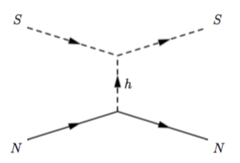
We begin with the final states for which the $SS$ annihilation proceeds by the $s$-channel exchange of $h$ and $H$ bosons only (the first diagram in Fig. 1). We write this annihilation cross sections by incorporating the expression for the SM Higgs decay width, setting the Higgs mass to the center of mass energy. For decays to $AB=f\bar{f}$ or $VV$, the resulting expression is:

$$\sigma v_{\rm rel} = \frac{2}{\sqrt{s}}\left(\frac{g_{SSh}g_{hAB}}{s-m_{h}^{2}}+\frac{g_{SSH}g_{HAB}}{s-m_{H}^{2}}\right)^{2}\frac{1}{g^{2}_{h_{SM}AB}}$$ (59)

$$\qquad\times\Gamma(m_{h_{SM}}=\sqrt{s},h_{SM}\rightarrow AB),$$

where $\Gamma$ is the decay width of a SM Higgs boson with a mass of $\sqrt{s}$ into final state $AB$. This decay width is calculated using the usual SM formulas.

We must also include the final state with one $H_{3}$ scalar and one vector boson. The cross section of this process when $\sqrt{s}>m_{3}+m_{V}$ is:

$$\sigma v_{\rm rel} = \frac{(s^{2}-2s(m_{3}^{2}+m_{V}^{2})+(m_{3}^{2}-m_{V}^{2})^{2})^{\frac{3}{2}}}{8\pi s^{2}m_{W}^{2}}$$ (60)

$$\qquad\times\left(\frac{g_{SSh}g_{hH_{3}V}}{s-m_{h}^{2}}+\frac{g_{SSH}g_{HH_{3}V}}{s-m_{H}^{2}}\right)^{2}.$$

When $\sqrt{s}<m_{3}+m_{V}$, we include the offshell process $SS\rightarrow V^{*}H_{3}$, whose cross section is given by

$$\sigma v_{\rm rel}=\left(\frac{g_{SSh}g_{hH_{3}V}}{s-m_{h}^{2}}+\frac{g_{SSH}g_{HH_{3}V}}{s-m_{H}^{2}}\right)^{2}\delta_{V}\frac{3m_{V}^{2}}{8\pi^{3}v^{2}}G_{ij},$$ (61)

where GMCALC ; Djouadi:1995gv ; Akeroyd:1998dt

$$G_{ij}= \frac{1}{4}\left[{2(-1+k_{j}-k_{i})\sqrt{\lambda_{ij}}\left(\frac{\pi}{2}+\arctan\left(\frac{k_{j}(1-k_{j}+k_{i})-\lambda_{ij}}{(1-k_{i})\sqrt{\lambda_{ij}}}\right)\right)}\right.$$

$$\qquad\left.{+(\lambda_{ij}-2k_{i})\log k_{i}+\frac{1}{3}(1-k_{i})\left(5(1+k_{i})-4k_{j}+\frac{2\lambda_{ij}}{k_{j}}\right)}\right],$$ (62)

with

$$\delta_{W}=\frac{3}{2},\qquad\delta_{Z}=3\left(\frac{7}{12}-\frac{10}{9}s_{W}^{2}+\frac{40}{27}s_{W}^{4}\right).$$ (63)

Here $k_{i}=m_{3}^{2}/s$, $k_{j}=m_{V}^{2}/s$, $s_{W}$ is the sine of the weak mixing angle, and $\lambda_{ij}=-1+2k_{i}+2k_{j}-(k_{i}-k_{i})^{2}$.

Figure 1: Feynman diagrams for $SS$ annihilation. In the first, the final state can be any allowed pair of SM particles or GM scalars. However, in the second and third diagrams, only scalar final states can appear. Crossed diagrams (not shown) are also included in the calculation.

IV.1.2 Final states involving $H_{3}$ or $H_{5}$ pairs

We now compute the $SS$ annihilation cross sections into final states that consist of neutral or charged $H_{3}$ and $H_{5}$ scalars. The possible final states considered here are:

$$(H_{3}^{0},H_{3}^{0}),(H_{3}^{+},H_{3}^{-}),(H_{5}^{0},H_{5}^{0}),(H_{5}^{+},H_{5}^{-}),(H_{5}^{++},H_{5}^{--}).$$ (64)

Since the two particles in each of these final states have the same mass, we will label it as $m_{i}$. Annihilation into these final states proceeds via $s$-channel and four-point diagrams (the first two diagrams in Fig. 1). The cross section for final-state particles $h_{1}$ and $h_{2}$ is given by:

$$\sigma v_{\rm rel}=\delta_{12}\frac{(s-4m_{h_{1}}^{2})^{\frac{1}{2}}}{16\pi s^{\frac{3}{2}}}$$ (65)

$$\times\left(g_{SSh_{1}h_{2}}+\frac{g_{SSh}g_{hh_{1}h_{2}}}{s-m_{h}^{2}}+\frac{g_{SSH}g_{Hh_{1}h_{2}}}{s-m_{H}^{2}}\right)^{2},$$

where $\delta_{12}=1/2$ for identical final-state particles $h_{1}=h_{2}$ and $\delta_{12}=1$ for non-identical final-state particles.

IV.1.3 $(h,H)$, $(h,h)$ and $(H,H)$ final states

The cross sections with $(h,H)$, $(h,h)$ or $(H,H)$ in the final state proceed via $s$-channel, four-point, and $t$- and $u$-channel diagrams (all the diagrams in Fig. 1 plus the crossed diagram). For non-identical $h_{i},h_{j}$ in the final state, we obtain:

$$\sigma v_{\rm rel}=\frac{\sqrt{s^{2}+(m_{h_{j}}^{2}-m_{h_{i}}^{2})^{2}-2s(m_{h_{j}}^{2}+m_{h_{i}}^{2})}}{16\pi s^{2}}g(s),$$ (66)

and for identical particles in the final state, we obtain:

$$\sigma v_{\rm rel}=\frac{\sqrt{s-4m_{h_{i}}^{2}}}{32\pi s^{3/2}}g(s),$$ (67)

where $g$, $a$, $b$, $c$, and $d$ are defined as follows:

$$g(s)= 2a^{2}+\frac{b^{2}}{c^{2}(c^{2}-d^{2})}+\frac{b(b-4ac^{2})}{c^{3}d}\tanh^{-1}\left(\frac{d}{c}\right),$$ (68)

$$a= g_{SSh_{i}h_{j}}+\sum_{k}\frac{g_{SSh_{k}}g_{h_{k}h_{i}h_{j}}}{s-m_{h_{k}}^{2}},$$ (69)

$$b= 4g_{SSh_{i}}g_{SSh_{j}}(s-(m_{h_{i}}^{2}+m_{h_{j}}^{2})),$$ (70)

$$c^{2}= (s-m_{h_{j}}^{2}-m_{h_{i}}^{2})^{2},$$ (71)

$$d^{2}= \left(1-\frac{4m_{S}^{2}}{s}\right)\left((s-m_{h_{j}}^{2}+m_{h_{i}}^{2})^{2}-4sm_{h_{i}}^{2}\right),$$ (72)

where the sum in $a$ runs over $h_{k}=h,H$.

IV.2 Imposing Relic Density

Here we give details on how we impose the relic density as a constraint on $\lambda_{a}$ and $\lambda_{b}$. We first note that the thermally averaged cross section is a strictly increasing function of $|\lambda_{a}|$ and $|\lambda_{b}|$. In our numerical scans, we would like to be able to randomly select a particular linear combination of the couplings $\lambda_{a}$ and $\lambda_{b}$ and then scale them both until the correct relic density is obtained. After generating a scan point in the original GM model (see next section for details), we select the values of $\lambda_{a}$, $\lambda_{b}$ and $\mu_{S}^{2}$ as follows:

• First, generate a random angle $\theta_{\lambda}\in\left[-\frac{\pi}{2},\frac{\pi}{2}\right]$;

• Randomly select either the positive or negative solution for $\lambda_{a}$;

• Set $\lambda_{b}=\lambda_{a}\tan\theta_{\lambda}$;

• Generate a random mass $m_{S}>0$ GeV;

• Find a value of $\lambda_{a}$ that yields a relic density of $0.1064\leq\Omega_{DM}h^{2}\leq 0.1176$ Komatsu:2010fb ;

• Once the value of $\lambda_{a}$ is found we can find $\lambda_{b}$ and, in turn, $\mu_{S}^{2}$ using Eq. (24).

The first three steps allows us to select a particular linear combination of $\lambda_{a}$ and $\lambda_{b}$. Generating $m_{S}$ directly lets us avoid unphysical negative $m_{S}^{2}$ values regardless of the actual values of $\lambda_{a}$ and $\lambda_{b}$. Finally, numerically searching for the correct value of $\lambda_{a}$ is straightforward because $\sigma v_{\rm rel}$ is an increasing function of $\lambda_{a}$ and $\sigma v_{\rm rel}\rightarrow\infty$ when $\lambda_{a}\rightarrow\infty$ and $\sigma v_{\rm rel}\rightarrow 0$ when $\lambda_{a}\rightarrow 0$.

V Numerical Scan Procedure

To map out the allowed parameter space, we perform numerical scans. In these scans, we start by imposing the theoretical constraints and the relic density constraint. We then check whether the points pass the remaining experimental constraints. In the plots that follow, points that pass the experimental constraints will be blue, while points that fail at least one constraint will be red.

For the dimensionful parameters, the ranges we scan over are:

• $-4\times 10^{4}$ GeV${}^{2}\leq\mu_{3}^{2}\leq 10^{6}$ GeV²;

• $0\leq M_{1}\leq\max(3500~{}{\rm GeV},3.5\sqrt{|\mu_{3}^{2}|})$;

• $|M_{2}|\leq\max(250~{}{\rm GeV},1.3\sqrt{|\mu_{3}^{2}|})$, with either sign allowed;

• $0\leq m_{S}\leq 1000$ GeV, $0\leq m_{S}\leq 125$ GeV, or $56\leq m_{S}\leq 63$ GeV (see text below for explanation of these three regions).

The ranges for $M_{1}$ and $M_{2}$ are chosen to minimize the number of points generated which fail the theory constraints while still scanning the whole parameter space. The mass parameters $\mu_{3}^{2}$ and $m_{S}$ do not have upper bounds so we impose arbitrary bounds for the purpose of the scan. We perform a scan with $0\leq m_{S}\leq 1000$ GeV in order to obtain a general picture of the parameter space, one with $0\leq m_{S}\leq 125$ GeV in order to obtain higher statistics in the interesting low-$m_{S}$ region, and finally a smaller dedicated scan with $56\leq m_{S}\leq 63$ GeV to further investigate the Higgs pole region.

From these values, we calculate $\lambda_{1}$, $\mu_{2}^{2}$ and $\mu_{S}^{2}$, and all the masses and couplings, and then use the relic density to fix a random linear combination of $\lambda_{a}$ and $\lambda_{b}$.

VI Direct and indirect collider constraints on the GM model

Very low masses for $H_{3}^{0,\pm}$ and $H_{5}^{0,\pm,\pm\pm}$ can have a substantial effect on the dark matter relic abundance through annihilations into pairs of these scalars. We constrain these masses using direct experimental search limits as follows. LHC limits on anomalous like-sign dimuon production ATLAS:2014kca set a lower bound on the mass of a doubly-charged scalar decaying to like-sign $W$ boson pairs. This was studied in Ref. Kanemura:2014ipa for the Higgs Triplet Model HTM and recast into the GM model in Ref. Logan:2015xpa . This yields a lower bound $m_{5}\geq 76$ GeV, so long as $H_{3}$ is heavier than $H_{5}$ so that decays $H_{5}^{\pm\pm}\to W^{\pm}H_{3}^{\pm}$ do not compete with the decays into like-sign $W$ pairs. Searches for a charged Higgs boson at the CERN Large Electron-Positron (LEP) collider Searches:2001ac exclude charged Higgs masses below 78 GeV, assuming that the charged Higgs decays entirely into a combination of $\tau\nu$ and $cs$ final states. This limit can be applied to $H_{3}^{\pm}$ so long as decays $H_{3}^{\pm}\to W^{\pm}H_{5}^{0},ZH_{5}^{\pm}$ do not compete with the decays to fermions. This holds when $H_{5}$ is heavier than $H_{3}$. We therefore impose the lower bounds

$$m_{3}\geq 76~{}{\rm GeV},\qquad\qquad m_{5}\geq 76~{}{\rm GeV}.$$ (73)

Low $H_{3}^{\pm}$ masses can also be constrained from their effect on the loop-induced decay of $b\to s\gamma$. We use the “loose” constraint determined for the GM model in Ref. Hartling:2014aga , which is based on an experimental average from the Heavy Flavour Averaging Group Beringer:1900zz ; Asner:2010qj and a theoretical prediction from the public code SuperIso v3.3 Mahmoudi:2007vz . The $b\to s\gamma$ constraint sets a maximum value of $v_{\chi}$ as a function of $m_{3}$. Although this could potentially be constraining, all points in our numerical scan satisfied this constraint.

VII Constraints from dark matter

VII.1 Dark Matter Direct Detection

When a dark matter particle is in close proximity with a nucleon, there may be a scattering via the t-exchange of a Higgs boson. This transfer of momentum can be detected from the nucleon recoil so that experimental limits can be used to constrain our model. In our model, this process proceeds via exchange of a virtual $h$ or $H$ as shown in Fig. 2.

Figure 2: Feynman diagram for direct detection via t-channel Higgs exchange in $SN\to SN$ scattering. There is a second diagram in which $h$ is replaced by $H$.

The spin-independent cross section for the scattering of a scalar dark matter particle $S$ off of a single nucleon is given by

$$\sigma=\left(\frac{g_{SSh}c_{\alpha}}{m_{h}^{2}c_{H}}+\frac{g_{SSH}s_{\alpha}}{m_{H}^{2}c_{H}}\right)^{2}\frac{f_{N}^{2}m_{N}^{4}}{4\pi(m_{N}+m_{S})^{2}v^{2}},$$ (74)

where we neglect the momentum transfer relative to the $h$ or $H$ mass, $c_{H}$ was defined in Eq. (20), $c_{\alpha}\equiv\cos\alpha$, $s_{\alpha}\equiv\sin\alpha$, and $f_{N}$ is the nucleon vertex factor Cline:2013gha ,

$$f_{N}=\sum_{q}f_{q}=\sum_{q}\frac{m_{q}}{m_{N}}<N|\bar{q}q|N>,$$ (75)

where the sum is over all quark flavours, and the Feynman rule for the Higgs-nucleon vertex is $-if_{N}m_{N}/v$. We follow Ref. Cline:2013gha in using $f_{N}=0.30\pm 0.03$ and $m_{N}=(m_{n}+m_{p})/2=938.95$ MeV.

Figure 3: Direct detection cross section as a function of $m_{S}$. The top plot is a zoom of the low-$m_{S}$ region while the bottom plot shows the full $m_{S}$ range scanned. The red (grey) points are eliminated by direct or indirect dark matter detection measurements and the blue (black) points are the remaining ones that are allowed. On the right side of the figures, starting at the top are the exclusion limits from LUX (solid magenta) Akerib:2016vxi , as well as projected sensitivities of DEAP-3600 (dashed green) Amaudruz:2014nsa , and XENON1T (dashed brown) Cushman:2013zza . The yellow shaded region below the lowest line is the coherent neutrino scattering background (“neutrino floor”) Billard:2013qya . Data files were taken from the DMTools website DMtools .

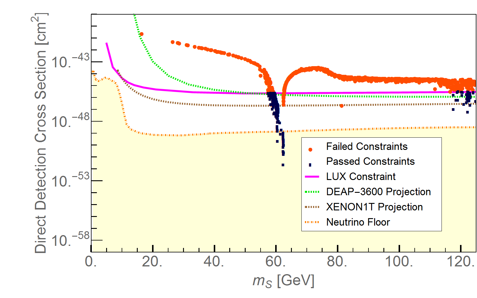
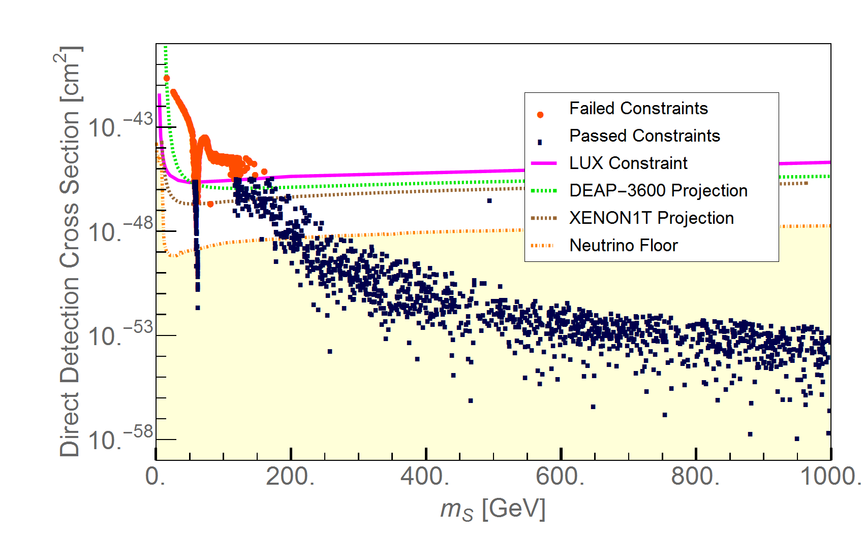
In Fig. 3 we illustrate the effect of the direct detection constraints on our model. The scan points shown are those that satisfy the theoretical constraints and yield the correct dark matter relic abundance. The blue points satisfy the constraints from the dark matter direct detection experiments as well as limits from indirect detection (see next subsection), while the red points fail those constraints. The current most stringent direct-detection cross section limit comes from the LUX experiment Akerib:2016vxi and is shown as the solid magenta line in Fig. 3. As can be seen, this constraint is responsible for excluding the great majority of the red (excluded) points in our scan, except for a small collection of points on the higher-mass side of the Higgs pole at $m_{h}/2=62.5$ GeV. We also show the projected limits from DEAP-3600 Amaudruz:2014nsa (dotted green) and XENON1T Cushman:2013zza (dotted brown), as well as the “neutrino floor” (yellow shaded region) below which coherent neutrino scattering becomes an irreducible background to the dark matter direct detection experiments Billard:2013qya .

VII.2 Dark matter indirect detection

Dwarf spheroidal satellite galaxies (dSphs) are typically dark matter dominated so are a good place to study dark matter. The Fermi collaboration has acquired 6 years worth of data observing 15 dSphs and have released bounds for WIMP dark matter annihilation based on their gamma ray flux. They considered the following representative final states for the dark matter annihilation: $e^{+}e^{-}$, $\mu^{+}\mu^{-}$, $\tau^{+}\tau^{-}$, $u\bar{u}$, $b\bar{b}$, and $W^{+}W^{-}$ FermiLAT .

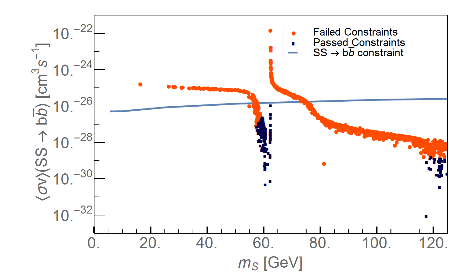
We can translate the Fermi bounds into constraints on our model by considering the branching ratio of the singlet annihilation to these final states. Although all of the final states are considered in our analysis, the strongest constraint comes from the $b\bar{b}$ final state for singlet scalar masses just below half the $h$ mass. Figure 4 shows the results of applying the $b\bar{b}$ constraint to the scan points. As can be seen, there is a sharp dip in the cross section followed by a sharp peak. The dip can be understood as coming from having to lower the values of $\lambda_{a}$ and $\lambda_{b}$ near the Higgs resonance, therefore lowering the $g_{SSh}$ coupling, in order to obtain the correct relic density. As the singlet mass approaches the Higgs pole, the thermal distribution during freeze-out pushes the center of mass energy above the pole. This results in increased values of $\lambda_{a}$ and $\lambda_{b}$ to obtain the correct relic density. However, since the temperature of dark matter is much lower today (we use the approximation that $v_{\rm rel}=0$), the increased coupling appears at a center of mass energy closer to the Higgs resonance and creates this peak. The indirect detection constraint thereby excludes a small collection of points on the heavier side of the $h$ pole dip in Fig. 3 that are not yet excluded by direct detection.

Figure 4: Present-day annihilation cross section for $SS\to b\bar{b}$ as a function of $m_{S}$. The blue (black) points are allowed while the red (grey) points are excluded by direct detection or dwarf spheroidal galaxy constraints. Points above the blue line are excluded by the dSphs $b\bar{b}$ constraint from the Fermi satellite FermiLAT . Fermi gives the thermally averaged cross section while we use the low velocity approximation and take $s=4m_{S}^{2}$.

VIII Contraints from Higgs boson properties

VIII.1 Higgs Invisible Width

When $m_{S}<m_{h,H}/2$, the decay of the Higgs boson to two dark matter candidates is kinematically accessible. For convenience we define:

$$\kappa_{f}^{h} =\frac{g_{hf\bar{f}}}{g^{SM}_{hf\bar{f}}}=\frac{c_{\alpha}}{c_{H}},$$

$$\kappa_{V}^{h} =\frac{g_{hVV}}{g^{SM}_{hVV}}=c_{\alpha}s_{H}-\sqrt{\frac{8}{3}}s_{\alpha}s_{H},$$

$$\kappa_{\gamma}^{h} =\left[\frac{\Gamma(h\rightarrow\gamma\gamma)}{\Gamma^{SM}(h\rightarrow\gamma\gamma)}\right]^{1/2}.$$ (76)

Note that $\kappa_{f}^{h}$ is the same for all fermions and $\kappa_{V}^{h}$ is the same for $V=Z$ and $W^{\pm}$. $\Gamma(h\rightarrow\gamma\gamma)$ receives contributions from $H_{3}^{+}$, $H_{5}^{+}$, and $H_{5}^{++}$ in addition to the modified $ht\bar{t}$ and $hWW$ couplings. The expression for the width of this process is

$$\Gamma(h\to{\rm inv})=\frac{g_{SSh}^{2}}{32m_{h}^{2}\pi}\sqrt{m_{h}^{2}-4m_{S}^{2}}.$$ (77)

The most stringent LHC constraint on invisible Higgs decay comes from Higgs production in vector boson fusion (VBF). To compare with experiment, we therefore consider the ratio Aad:2015pla

$$\frac{\sigma_{VBF}{\rm BR}_{\rm inv}}{\sigma_{VBF}^{SM}}=\frac{(\kappa_{V}^{h})^{2}\Gamma(h\rightarrow{\rm inv})}{\Gamma_{\rm tot}}<0.29,$$ (78)

written in terms of the vector boson fusion (VBF) production cross section and the invisible branching ratio. In the total width $\Gamma_{\rm tot}$ of $h$ we include decays to $b\bar{b}$, $c\bar{c}$, $\tau\tau$, $gg$, $WW^{*}$, $ZZ^{*}$, $\gamma\gamma$, and $SS$ as computed above.

Figure 5: Cross section times branching ratio for $h$ production in vector boson fusion followed by invisible decays to $SS$, normalized to the SM cross section, as a function of $m_{S}$. The blue (black) points are allowed while the red (grey) points are excluded by direct detection or dwarf spheroidal galaxy constraints. Points above the blue line are excluded by the ATLAS limit on $\sigma_{VBF}{\rm BR}_{\rm inv}/\sigma^{SM}_{VBF}$ Aad:2015pla .

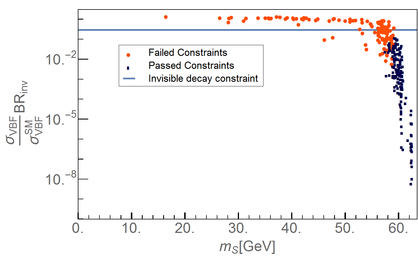
The ratio in Eq. (78) is shown in Fig. 5, plotted against $m_{S}$ in the kinematically allowed region. The experimental constraint of $\sigma_{VBF}{\rm BR}_{\rm inv}/\sigma^{SM}_{VBF}<0.29$ Aad:2015pla is shown as the horizontal blue line. The bound from invisible Higgs decays is currently not as strong as the constraints from direct detection of dark matter.

VIII.2 Higgs Couplings and Signal Strength

We finally apply the latest combined measurements of Higgs couplings from CMS and ATLAS from Run 1 of the LHC ATLAS:2016HiggsSignals to our model. In this section we discard the points that are excluded by dark matter direct detection or indirect detection constraints. We will find that the Higgs coupling measurements exclude a significant fraction of the remaining points, in particular those for which the $h$ coupling to fermion or vector boson pairs is sufficiently different from the SM.

We write the cross sections and branching ratios in terms of the appropriate SM values and the $\kappa$ factors defined in Eq. (76) as follows:

$$\sigma(AB\rightarrow h) =(\kappa^{h}_{AB})^{2}\sigma^{SM}(AB\rightarrow h),$$

$${\rm BR}(h\rightarrow AB) =(\kappa^{h}_{AB})^{2}\frac{\Gamma^{SM}_{\rm tot}}{\Gamma_{\rm tot}}{\rm BR}^{SM}(h\rightarrow AB),$$ (79)

where $\kappa^{h}_{g}=\kappa^{h}_{f}$.

We compute a $\chi^{2}$ using the ATLAS+CMS combined results for the LHC Run 1 Higgs properties from Table 9 and the correlation matrix from Fig. 28 of Ref. ATLAS:2016HiggsSignals . The inputs we use in this analysis are: $\sigma(gg\rightarrow h\rightarrow ZZ)$, $\sigma_{\rm VBF}/\sigma_{gg\rm F}$, $\sigma_{Wh}/\sigma_{gg\rm F}$, $\sigma_{Zh}/\sigma_{gg\rm F}$, $\sigma_{tth}/\sigma_{gg\rm F}$, ${\rm BR}^{WW}/{\rm BR}^{ZZ}$, ${\rm BR}^{\gamma\gamma}/{\rm BR}^{ZZ}$, ${\rm BR}^{\tau\tau}/{\rm BR}^{ZZ}$, and ${\rm BR}^{bb}/{\rm BR}^{ZZ}$. We start by symmetrizing the uncertainties for a given observable by taking the root mean square of the asymmetric uncertainties. We then construct the variance matrix $V$ from these symmetrized uncertainties and the correlation matrix and define:

$$\chi^{2}=(\mathbf{x}-\mathbf{y})^{T}V^{-1}(\mathbf{x}-\mathbf{y}),$$ (80)

where $\mathbf{x}$ is a vector of the experimental best fit values and $\mathbf{y}$ is a vector of calculated values using the kappas and the SM predictions from Table 9 of Ref. ATLAS:2016HiggsSignals . Using the SM predictions for $\mathbf{y}$ we get:

$$\chi^{2}_{SM}=30.0448.$$ (81)

We will consider a point in our model to be consistent with the experimental measurements of these observables if:

$$\Delta\chi^{2}\equiv|\chi^{2}-\chi^{2}_{SM}|<4.$$

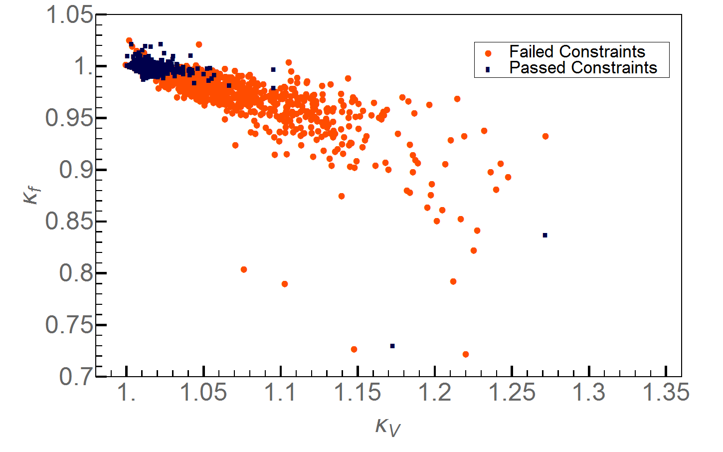
We apply the constraints from the Higgs couplings fit only to the points that have passed all previous dark matter constraints. Figure 6 shows the points that pass (blue/black) and those that fail (red/gray) the $\chi^{2}$ constraint from Higgs couplings in the $\kappa_{V}^{h}$-$\kappa_{f}^{h}$ plane. The Higgs coupling measurements exclude points for which $\kappa_{V}^{h}$ or $\kappa_{f}^{h}$ deviate too much from their SM value of 1.

Figure 6: Couplings of $h$ to fermions ($\kappa_{f}^{h}$) and $W$ and $Z$ bosons ($\kappa_{V}^{h}$) normalized to their SM values, for only the points allowed by the dark matter direct and indirect detection constraints. The dark blue (black) points satisfy the $\Delta\chi^{2}<4$ condition for the Higgs coupling measurements from the LHC Run 1 data ATLAS:2016HiggsSignals , while the red (grey) points fail this condition.

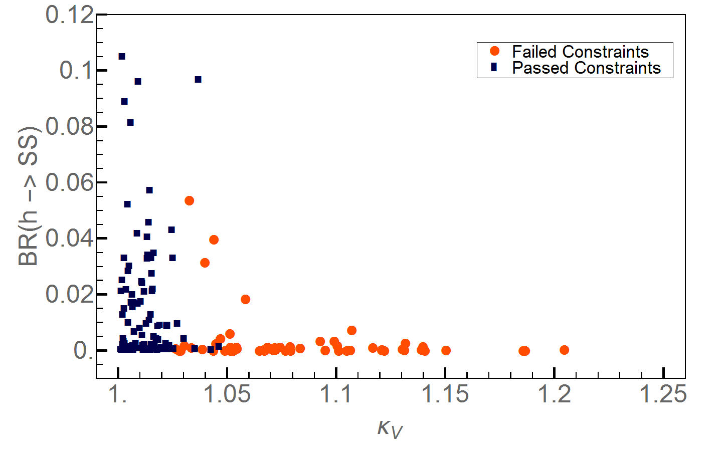
Of particular interest for Higgs phenomenology is the case where the singlet is lighter than half the Higgs mass. This allows the Higgs to decay to a pair of singlets which would then escape the detector. Figure 7 shows the branching ratio of $h\rightarrow SS$ as a function of $\kappa_{V}^{h}$ for the points that passed all previous constraints and have a singlet mass less than half the Higgs mass.

Figure 7: Branching ratio of $h\to SS$ as a function of $\kappa_{V}^{h}$, for only the points allowed by the dark matter direct and indirect detection constraints and for which $m_{S}<m_{h}/2$. The dark blue (black) points satisfy the $\Delta\chi^{2}<4$ condition for the Higgs coupling measurements from the LHC Run 1 data ATLAS:2016HiggsSignals , while the red (grey) points fail this condition.

The only observable in the $\chi^{2}$ analysis that is sensitive to the total decay width of the Higgs boson is the $\sigma(gg\rightarrow h\rightarrow ZZ)$ cross section, because the total width cancels out in all the other inputs. In particular, we have:

$$\frac{\sigma(gg\rightarrow h\rightarrow ZZ)}{\sigma^{SM}(gg\rightarrow h\rightarrow ZZ)}=\left(\kappa_{f}^{h}\kappa_{V}^{h}\right)^{2}\frac{\Gamma^{SM}_{\rm tot}}{\Gamma_{\rm tot}}.$$ (82)

This observable allows us to potentially distinguish between our model and the original GM model without the scalar singlet dark matter candidate. In Fig. 8 we plot this observable versus $\kappa_{V}^{h}$ for the points that survive the $\Delta\chi^{2}<4$ constraint and for which the mass of the singlet is less than half the Higgs mass, so that $h\to SS$ is kinematically allowed. These are the blue (black) points. We then take the same points, set $\mu_{s}=\lambda_{a}=\lambda_{b}=\lambda_{S}=0$ while keeping the other Lagrangian parameters fixed, and remove the singlet from the theory. These points are plotted in red (gray). For these points the couplings $\kappa_{f}^{h}$, $\kappa_{V}^{h}$, and $\kappa_{\gamma}^{h}$ are the same as in the full model, but ${\rm BR}(h\to SS)$ (and its contribution to the Higgs total width) is eliminated.

Figure 8: Prediction for the cross section $\sigma(gg\to h\to ZZ)$ normalized to its SM value as a function of $\kappa_{V}^{f}$. The dark blue (black) points are the points that pass the dark matter direct and indirect detection constraints and satisfy the $\Delta\chi^{2}<4$ constraint from the Higgs coupling measurements. The red (gray) points are the same parameter points but with the $h\to SS$ decays switched off (see text for details) – these correspond to the predictions in the original GM model without the singlet scalar.

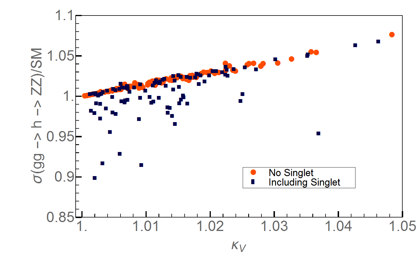
As can be seen, for the original GM model without the singlet, the red points fall roughly along a line due to the correlation between $\kappa_{V}^{h}$ and ${\rm BR}(h\to ZZ)$ after the rest of the Higgs coupling measurements are imposed. For the full GM model with the singlet scalar dark matter candidate, however, some of the points are scattered downward to smaller values of $\sigma(gg\to h\to ZZ)/{\rm SM}$, due to the suppression of ${\rm BR}(h\to ZZ)$ by the competing $h\to SS$ decay mode. These are the same points for which ${\rm BR}(h\to SS)$ is visibly above zero in Fig. 7. This offers a second way to potentially discriminate between the original GM model and its scalar singlet extension through an improved precision on the measurement of $\sigma(gg\rightarrow h\rightarrow ZZ)$, when $m_{S}<m_{h}/2$.

IX Conclusions

In this paper we studied the addition of a scalar dark matter candidate to the Georgi-Machacek model. This provides a concrete implementation of a scenario in which the Higgs couplings to vector boson and fermion pairs can be enhanced while a new, non-SM decay mode is also present, thereby allowing an exploration of the interplay of Higgs production and decay constraints. We showed that the dark matter candidate in this model can be made to respect all current constraints while allowing for a sizable (up to 10%) branching ratio for the Higgs to the dark matter candidate in certain areas of parameter space.

The model consists of the Georgi-Machacek model with the addition of a real singlet which has a $Z_{2}$ symmetry to make it stable. We first studied the theoretical constraints on the new parameters by imposing tree-level unitarity in $2\rightarrow 2$ scalar scattering amplitudes, requiring that the potential is bounded from below, and requiring that deeper custodial $SU(2)$-violating minima are absent. We found that we could translate all the constraints from the original GM model to our extended model and simply add a few new constraints on the new Lagrangian parameters.

We performed a numerical scan over the Lagrangian parameters, imposing the theoretical constraints and requiring that the singlet scalar accounts for all of the dark matter in the universe through thermal freeze-out. We identified the parameter regions that satisfy the constraints from dark matter direct-detection searches as well as the indirect constraints from gamma ray measurements of dwarf spheroidal galaxies. This constrained the dark matter mass to be either near the Higgs pole for resonant annihilation (57-62 GeV) or mostly above about 120 GeV. We also saw that for parameter values where the dark matter mass was near the Higgs pole we could attain a sizable branching ratio for $h\rightarrow SS$; however, after imposing the dark matter constraints, the current limit on the Higgs invisible decays does not further constrain the model.

We finally studied the constraints from the LHC Run 1 Higgs coupling measurements. While these measurements further constrain the parameter space, they do so mostly by constraining the $hf\bar{f}$, $hVV$, and $h\gamma\gamma$ couplings. The Higgs coupling measurements are not yet precise enough to be sensitive to the modification of signal rates by the presence of the $h\to SS$ decay mode, so that the constraints from Higgs measurements are so far the same as they would be in the original GM model without the singlet scalar.

The allowed region of parameter space that we identified can be further probed in the future by the next generation of dark matter direct detection experiments, as well as improved precision on the invisible Higgs decay width and Higgs coupling measurements.

Appendix A Feynman rules for couplings involving $S$

A.1 Triple scalar couplings

The Feynman rules for couplings to $S$ are given by $-ig_{SSh_{i}}$ with all particles incoming and the couplings defined as follows:

$$g_{SSh} =-4\left(\lambda_{a}s_{\alpha}v_{\phi}+\sqrt{3}\lambda_{b}c_{\alpha}v_{\chi}\right),$$

$$g_{SSH} =-4\left(\lambda_{a}c_{\alpha}v_{\phi}+\sqrt{3}\lambda_{b}s_{\alpha}v_{\chi}\right),$$ (83)

where we use the notation $s_{\alpha}\equiv\sin\alpha$ and $c_{\alpha}\equiv\cos\alpha$.

A.2 Quartic scalar couplings

The Feynman rules for couplings to $S$ are given by $-ig_{SSs_{1}s_{2}}$ with all particles incoming and the couplings defined as follows:

$$g_{SShh} =-4\left(\lambda_{a}c^{2}_{\alpha}+\lambda_{b}s^{2}_{\alpha}\right),$$

$$g_{SSHH} =-4\left(\lambda_{a}s^{2}_{\alpha}+\lambda_{b}c^{2}_{\alpha}\right),$$

$$g_{SShH} =-4s_{\alpha}c_{\alpha}\left(\lambda_{a}-\lambda_{b}\right),$$

$$g_{SSG^{0}G^{0}} =g_{SSG^{+}G^{+*}}=-4\left(\lambda_{a}c^{2}_{H}+\lambda_{b}s^{2}_{H}\right),$$

$$g_{SSH_{3}^{0}H_{3}^{0}} =g_{SSH_{3}^{+}H_{3}^{+*}}=-4\left(\lambda_{a}s^{2}_{H}+\lambda_{b}c^{2}_{H}\right),$$

$$g_{SSG^{0}H_{3}^{0}} =g_{SSG^{+}H_{3}^{+*}}=g_{SSH_{3}^{+}G^{+*}}=-4s_{H}c_{H}\left(\lambda_{b}-\lambda_{a}\right),$$

$$g_{SSH_{5}^{0}H_{5}^{0}} =g_{SSH_{5}^{+}H_{5}^{+*}}=g_{SSH_{5}^{++}H_{5}^{++*}}=-4\lambda_{b},$$ (84)

where we use the notation $s_{H}\equiv\sin\theta_{H}$ and $c_{H}\equiv\cos\theta_{H}$, and $G^{0}$ and $G^{\pm}$ are the Goldstone bosons.

All other Feynman rules are identical to those in the original GM model and can be found in Appendix A of Ref. Hartling:2014zca

References

- (1) G. Aad et al. [ATLAS Collaboration], “Observation of a new particle in the search for the Standard Model Higgs boson with the ATLAS detector at the LHC,” Phys. Lett. B 716, 1 (2012) [arXiv:1207.7214 [hep-ex]]; S. Chatrchyan et al. [CMS Collaboration], “Observation of a new boson at a mass of 125 GeV with the CMS experiment at the LHC,” Phys. Lett. B 716, 30 (2012) [arXiv:1207.7235 [hep-ex]].
- (2) A. David et al. [LHC Higgs Cross Section Working Group Collaboration], “LHC HXSWG interim recommendations to explore the coupling structure of a Higgs-like particle,” arXiv:1209.0040 [hep-ph].
- (3) D. Zeppenfeld, R. Kinnunen, A. Nikitenko and E. Richter-Was, “Measuring Higgs boson couplings at the CERN LHC,” Phys. Rev. D 62, 013009 (2000) [hep-ph/0002036]; A. Djouadi, R. Kinnunen, E. Richter-Was, H. U. Martyn, K. A. Assamagan, C. Balazs, G. Belanger and E. Boos et al., “The Higgs working group: Summary report,” hep-ph/0002258.
- (4) H. Baer, T. Barklow, K. Fujii, Y. Gao, A. Hoang, S. Kanemura, J. List and H. E. Logan et al., “The International Linear Collider Technical Design Report - Volume 2: Physics,” arXiv:1306.6352 [hep-ph].
- (5) H. Georgi and M. Machacek, “Doubly Charged Higgs Bosons,” Nucl. Phys. B 262, 463 (1985).
- (6) M. S. Chanowitz and M. Golden, “Higgs Boson Triplets With M() = M() ,” Phys. Lett. B 165, 105 (1985).
- (7) P. Galison, “Large Weak Isospin and the Mass,” Nucl. Phys. B 232, 26 (1984).
- (8) R. W. Robinett, “Extended Strongly Interacting Higgs Theories,” Phys. Rev. D 32, 1780 (1985).
- (9) H. E. Logan, “Radiative corrections to the vertex and constraints on extended Higgs sectors,” hep-ph/9906332.
- (10) S. Chang, C. A. Newby, N. Raj and C. Wanotayaroj, “Revisiting Theories with Enhanced Higgs Couplings to Weak Gauge Bosons,” Phys. Rev. D 86, 095015 (2012) [arXiv:1207.0493 [hep-ph]].
- (11) H. E. Logan and V. Rentala, “All the generalized Georgi-Machacek models,” Phys. Rev. D 92, no. 7, 075011 (2015) [arXiv:1502.01275 [hep-ph]].
- (12) J. Hisano and K. Tsumura, “Higgs boson mixes with an SU(2) septet representation,” Phys. Rev. D 87, 053004 (2013) [arXiv:1301.6455 [hep-ph]].
- (13) S. Kanemura, M. Kikuchi and K. Yagyu, “Probing exotic Higgs sectors from the precise measurement of Higgs boson couplings,” Phys. Rev. D 88, 015020 (2013) [arXiv:1301.7303 [hep-ph]].
- (14) C. Alvarado, L. Lehman and B. Ostdiek, “Surveying the Scope of the Scalar Septet Sector,” JHEP 1405, 150 (2014) [arXiv:1404.3208 [hep-ph]].
- (15) J. F. Gunion, R. Vega and J. Wudka, “Higgs triplets in the standard model,” Phys. Rev. D 42, 1673 (1990).
- (16) J. F. Gunion, R. Vega and J. Wudka, “Naturalness problems for and other large one loop effects for a standard model Higgs sector containing triplet fields,” Phys. Rev. D 43, 2322 (1991).
- (17) J. F. Gunion, H. E. Haber, G. L. Kane, and S. Dawson, The Higgs Hunter’s Guide (Westview, Boulder, Colorado, 2000).
- (18) H. E. Haber and H. E. Logan, “Radiative corrections to the vertex and constraints on extended Higgs sectors,” Phys. Rev. D 62, 015011 (2000) [hep-ph/9909335].
- (19) M. Aoki and S. Kanemura, “Unitarity bounds in the Higgs model including triplet fields with custodial symmetry,” Phys. Rev. D 77, 095009 (2008) [arXiv:0712.4053 [hep-ph]]; erratum Phys. Rev. D 89, 059902 (2014).
- (20) S. Godfrey and K. Moats, “Exploring Higgs Triplet Models via Vector Boson Scattering at the LHC,” Phys. Rev. D 81, 075026 (2010) [arXiv:1003.3033 [hep-ph]].
- (21) I. Low and J. Lykken, “Revealing the electroweak properties of a new scalar resonance,” JHEP 1010, 053 (2010) [arXiv:1005.0872 [hep-ph]]; I. Low, J. Lykken and G. Shaughnessy, “Have We Observed the Higgs (Imposter)?,” Phys. Rev. D 86, 093012 (2012) [arXiv:1207.1093 [hep-ph]].
- (22) H. E. Logan and M.-A. Roy, “Higgs couplings in a model with triplets,” Phys. Rev. D 82, 115011 (2010) [arXiv:1008.4869 [hep-ph]].
- (23) A. Falkowski, S. Rychkov and A. Urbano, “What if the Higgs couplings to and bosons are larger than in the Standard Model?,” JHEP 1204, 073 (2012) [arXiv:1202.1532 [hep-ph]].
- (24) C.-W. Chiang and K. Yagyu, “Testing the custodial symmetry in the Higgs sector of the Georgi-Machacek model,” JHEP 1301, 026 (2013) [arXiv:1211.2658 [hep-ph]].
- (25) C. Englert, E. Re and M. Spannowsky, “Triplet Higgs boson collider phenomenology after the LHC,” Phys. Rev. D 87, 095014 (2013) [arXiv:1302.6505 [hep-ph]].
- (26) R. Killick, K. Kumar and H. E. Logan, “Learning what the Higgs boson is mixed with,” Phys. Rev. D 88, 033015 (2013) [arXiv:1305.7236 [hep-ph]].
- (27) C. Englert, E. Re and M. Spannowsky, “Pinning down Higgs triplets at the LHC,” Phys. Rev. D 88, 035024 (2013) [arXiv:1306.6228 [hep-ph]].
- (28) C.-W. Chiang, A.-L. Kuo and K. Yagyu, “Enhancements of weak gauge boson scattering processes at the CERN LHC,” JHEP 1310, 072 (2013) [arXiv:1307.7526 [hep-ph]].
- (29) A. Efrati and Y. Nir, “What if ,” arXiv:1401.0935 [hep-ph].
- (30) K. Hartling, K. Kumar and H. E. Logan, “The decoupling limit in the Georgi-Machacek model,” Phys. Rev. D 90, 015007 (2014) [arXiv:1404.2640 [hep-ph]].
- (31) C. W. Chiang and T. Yamada, “Electroweak phase transition in Georgi Machacek model,” Phys. Lett. B 735, 295 (2014) [arXiv:1404.5182 [hep-ph]].
- (32) C. W. Chiang, S. Kanemura and K. Yagyu, “Novel constraint on the parameter space of the Georgi-Machacek model with current LHC data,” Phys. Rev. D 90, no. 11, 115025 (2014) [arXiv:1407.5053 [hep-ph]].
- (33) S. I. Godunov, M. I. Vysotsky and E. V. Zhemchugov, “Double Higgs production at LHC, see-saw type II and Georgi-Machacek model,” J. Exp. Theor. Phys. 120, no. 3, 369 (2015) [arXiv:1408.0184 [hep-ph]].
- (34) K. Hartling, K. Kumar and H. E. Logan, “Indirect constraints on the Georgi-Machacek model and implications for Higgs boson couplings,” Phys. Rev. D 91, no. 1, 015013 (2015) [arXiv:1410.5538 [hep-ph]].
- (35) C. W. Chiang and K. Tsumura, “Properties and searches of the exotic neutral Higgs bosons in the Georgi-Machacek model,” arXiv:1501.04257 [hep-ph].
- (36) S. I. Godunov, M. I. Vysotsky and E. V. Zhemchugov, “Suppression of decay channels in the Georgi-Machacek model,” arXiv:1505.05039 [hep-ph].
- (37) S. Chang and J. G. Wacker, “Little Higgs and custodial SU(2),” Phys. Rev. D 69, 035002 (2004) [hep-ph/0303001].
- (38) S. Chang, “A ‘Littlest Higgs’ model with custodial SU(2) symmetry,” JHEP 0312, 057 (2003) [hep-ph/0306034].
- (39) L. Cort, M. Garcia and M. Quiros, “Supersymmetric Custodial Triplets,” Phys. Rev. D 88, 075010 (2013) [arXiv:1308.4025 [hep-ph]].
- (40) M. Garcia-Pepin, S. Gori, M. Quiros, R. Vega, R. Vega-Morales and T. T. Yu, “Supersymmetric Custodial Higgs Triplets and the Breaking of Universality,” Phys. Rev. D 91, no. 1, 015016 (2015) [arXiv:1409.5737 [hep-ph]].
- (41) S. El Hedri, P. J. Fox and J. G. Wacker, “Exploring the dark side of the top Yukawa,” arXiv:1311.6488 [hep-ph].
- (42) G. B. Gelmini, “TASI 2014 Lectures: The Hunt for Dark Matter,” arXiv:1502.01320 [hep-ph].
- (43) M. J. G. Veltman and F. J. Yndurain, “Radiative Corrections To W W Scattering,” Nucl. Phys. B 325, 1 (1989).
- (44) V. Silveira and A. Zee, “Scalar Phantoms,” Phys. Lett. B 161, 136 (1985).
- (45) J. McDonald, “Gauge singlet scalars as cold dark matter,” Phys. Rev. D 50, 3637 (1994) [hep-ph/0702143].
- (46) C. P. Burgess, M. Pospelov and T. ter Veldhuis, “The Minimal model of nonbaryonic dark matter: A Singlet scalar,” Nucl. Phys. B 619, 709 (2001) [hep-ph/0011335].
- (47) J. McDonald, “Thermally generated gauge singlet scalars as selfinteracting dark matter,” Phys. Rev. Lett. 88, 091304 (2002) [hep-ph/0106249].
- (48) V. Barger, P. Langacker, M. McCaskey, M. J. Ramsey-Musolf and G. Shaughnessy, “LHC Phenomenology of an Extended Standard Model with a Real Scalar Singlet,” Phys. Rev. D 77, 035005 (2008) [arXiv:0706.4311 [hep-ph]].
- (49) A. Goudelis, Y. Mambrini and C. Yaguna, “Antimatter signals of singlet scalar dark matter,” JCAP 0912, 008 (2009) [arXiv:0909.2799 [hep-ph]].
- (50) M. Gonderinger, Y. Li, H. Patel and M. J. Ramsey-Musolf, “Vacuum Stability, Perturbativity, and Scalar Singlet Dark Matter,” JHEP 1001, 053 (2010) [arXiv:0910.3167 [hep-ph]].
- (51) X. G. He, T. Li, X. Q. Li, J. Tandean and H. C. Tsai, “The Simplest Dark-Matter Model, CDMS II Results, and Higgs Detection at LHC,” Phys. Lett. B 688, 332 (2010) [arXiv:0912.4722 [hep-ph]].
- (52) S. Profumo, L. Ubaldi and C. Wainwright, “Singlet Scalar Dark Matter: monochromatic gamma rays and metastable vacua,” Phys. Rev. D 82, 123514 (2010) [arXiv:1009.5377 [hep-ph]].
- (53) C. E. Yaguna, “The Singlet Scalar as FIMP Dark Matter,” JHEP 1108, 060 (2011) [arXiv:1105.1654 [hep-ph]].
- (54) A. Drozd, B. Grzadkowski and J. Wudka, “Multi-Scalar-Singlet Extension of the Standard Model - the Case for Dark Matter and an Invisible Higgs Boson,” JHEP 1204, 006 (2012), erratum JHEP 1411, 130 (2014) [arXiv:1112.2582 [hep-ph]].
- (55) A. Djouadi, O. Lebedev, Y. Mambrini and J. Quevillon, “Implications of LHC searches for Higgs–portal dark matter,” Phys. Lett. B 709, 65 (2012) [arXiv:1112.3299 [hep-ph]].
- (56) M. Kadastik, K. Kannike, A. Racioppi and M. Raidal, “Implications of the 125 GeV Higgs boson for scalar dark matter and for the CMSSM phenomenology,” JHEP 1205, 061 (2012) [arXiv:1112.3647 [hep-ph]].
- (57) A. Djouadi, A. Falkowski, Y. Mambrini and J. Quevillon, “Direct Detection of Higgs-Portal Dark Matter at the LHC,” Eur. Phys. J. C 73, 2455 (2013) [arXiv:1205.3169 [hep-ph]].
- (58) K. Cheung, Y. L. S. Tsai, P. Y. Tseng, T. C. Yuan and A. Zee, “Global Study of the Simplest Scalar Phantom Dark Matter Model,” JCAP 1210, 042 (2012) [arXiv:1207.4930 [hep-ph]].
- (59) P. H. Damgaard, D. O’Connell, T. C. Petersen and A. Tranberg, “Constraints on New Physics from Baryogenesis and Large Hadron Collider Data,” Phys. Rev. Lett. 111, 221804 (2013) [arXiv:1305.4362 [hep-ph]].
- (60) J. M. Cline, K. Kainulainen, P. Scott and C. Weniger, “Update on scalar singlet dark matter,” Phys. Rev. D 88, 055025 (2013) [arXiv:1306.4710 [hep-ph]].
- (61) S. Baek, P. Ko and W. I. Park, “Invisible Higgs Decay Width vs. Dark Matter Direct Detection Cross Section in Higgs Portal Dark Matter Models,” Phys. Rev. D 90, 055014 (2014) [arXiv:1405.3530 [hep-ph]].
- (62) L. Feng, S. Profumo and L. Ubaldi, “Closing in on singlet scalar dark matter: LUX, invisible Higgs decays and gamma-ray lines,” JHEP 1503, 045 (2015) [arXiv:1412.1105 [hep-ph]].
- (63) R. Campbell, S. Godfrey, H. E. Logan, A. D. Peterson and A. Poulin, “Implications of the observation of dark matter self-interactions for singlet scalar dark matter,” Phys. Rev. D 92, no. 5, 055031 (2015) [arXiv:1505.01793 [hep-ph]].
- (64) X. G. He, T. Li, X. Q. Li, J. Tandean and H. C. Tsai, “Constraints on Scalar Dark Matter from Direct Experimental Searches,” Phys. Rev. D 79, 023521 (2009) [arXiv:0811.0658 [hep-ph]].
- (65) B. Grzadkowski and P. Osland, “Tempered Two-Higgs-Doublet Model,” Phys. Rev. D 82, 125026 (2010) [arXiv:0910.4068 [hep-ph]].
- (66) H. E. Logan, “Dark matter annihilation through a lepton-specific Higgs boson,” Phys. Rev. D 83, 035022 (2011) [arXiv:1010.4214 [hep-ph]].
- (67) M. S. Boucenna and S. Profumo, “Direct and Indirect Singlet Scalar Dark Matter Detection in the Lepton-Specific two-Higgs-doublet Model,” Phys. Rev. D 84, 055011 (2011) [arXiv:1106.3368 [hep-ph]].
- (68) X. G. He, B. Ren and J. Tandean, “Hints of Standard Model Higgs Boson at the LHC and Light Dark Matter Searches,” Phys. Rev. D 85, 093019 (2012) [arXiv:1112.6364 [hep-ph]].
- (69) Y. Bai, V. Barger, L. L. Everett and G. Shaughnessy, “Two-Higgs-doublet-portal dark-matter model: LHC data and Fermi-LAT 135 GeV line,” Phys. Rev. D 88, 015008 (2013) [arXiv:1212.5604 [hep-ph]].
- (70) X. G. He and J. Tandean, “Low-Mass Dark-Matter Hint from CDMS II, Higgs Boson at the LHC, and Darkon Models,” Phys. Rev. D 88, 013020 (2013) [arXiv:1304.6058 [hep-ph]].
- (71) Y. Cai and T. Li, “Singlet dark matter in a type II two Higgs doublet model,” Phys. Rev. D 88, 115004 (2013) [arXiv:1308.5346 [hep-ph]].
- (72) C. Y. Chen, M. Freid and M. Sher, “Next-to-minimal two Higgs doublet model,” Phys. Rev. D 89, 075009 (2014) [arXiv:1312.3949 [hep-ph]].
- (73) L. Wang and X. F. Han, “A simplified 2HDM with a scalar dark matter and the galactic center gamma-ray excess,” Phys. Lett. B 739, 416 (2014) [arXiv:1406.3598 [hep-ph]].
- (74) A. Drozd, B. Grzadkowski, J. F. Gunion and Y. Jiang, “Extending two-Higgs-doublet models by a singlet scalar field - the Case for Dark Matter,” JHEP 1411, 105 (2014) [arXiv:1408.2106 [hep-ph]].
- (75) E. W. Kolb and M. S. Turner, “The Early Universe,” Front. Phys. 69, 1 (1990).
- (76) D.S. Akerib et al., “Results from a search for dark matter in LUX with 332 live days of exposure,” [arXiv:1608.07648 [astro-ph.CO]].
- (77) A. Arhrib, R. Benbrik, M. Chabab, G. Moultaka, M. C. Peyranere, L. Rahili and J. Ramadan, “The Higgs Potential in the Type II Seesaw Model,” Phys. Rev. D 84, 095005 (2011) [arXiv:1105.1925 [hep-ph]].
- (78) P. Gondolo and G. Gelmini, “Cosmic abundances of stable particles: Improved analysis,” Nucl. Phys. B 360, 145 (1991).
- (79) J. Edsjo and P. Gondolo, “Neutralino relic density including coannihilations,” Phys. Rev. D 56, 1879 (1997) [hep-ph/9704361].
- (80) A. Djouadi, J. Kalinowski and P. M. Zerwas, “Two and three-body decay modes of SUSY Higgs particles,” Z. Phys. C 70, 435 (1996) [hep-ph/9511342].
- (81) A. G. Akeroyd, “Three body decays of Higgs bosons at LEP-2 and application to a hidden fermiophobic Higgs,” Nucl. Phys. B 544, 557 (1999) [hep-ph/9806337].
- (82) K. Hally, K. Kumar and H. E. Logan, “GMCALC: a calculator for the Georgi-Machacek model,” [arXiv:1412.7387 [hep-ph]].
- (83) E. Komatsu et al. [WMAP Collaboration], “Seven-Year Wilkinson Microwave Anisotropy Probe (WMAP) Observations: Cosmological Interpretation,” Astrophys. J. Suppl. 192, 18 (2011) [arXiv:1001.4538 [astro-ph.CO]].
- (84) G. Aad et al. [ATLAS Collaboration], “Search for anomalous production of prompt same-sign lepton pairs and pair-produced doubly charged Higgs bosons with TeV collisions using the ATLAS detector,” JHEP 1503, 041 (2015) [arXiv:1412.0237 [hep-ex]].
- (85) S. Kanemura, M. Kikuchi, H. Yokoya and K. Yagyu, “LHC Run-I constraint on the mass of doubly charged Higgs bosons in the same-sign diboson decay scenario,” PTEP 2015, 051B02 (2015) [arXiv:1412.7603 [hep-ph]].
- (86) J. Schechter and J. W. F. Valle, “Neutrino Masses in SU(2) x U(1) Theories,” Phys. Rev. D 22, 2227 (1980); T. P. Cheng and L. F. Li, “Neutrino Masses, Mixings and Oscillations in SU(2) x U(1) Models of Electroweak Interactions,” Phys. Rev. D 22, 2860 (1980); M. Magg and C. Wetterich, “Neutrino Mass Problem and Gauge Hierarchy,” Phys. Lett. B 94, 61 (1980); G. Lazarides, Q. Shafi and C. Wetterich, “Proton Lifetime and Fermion Masses in an SO(10) Model,” Nucl. Phys. B 181, 287 (1981); R. N. Mohapatra and G. Senjanovic, “Neutrino Masses and Mixings in Gauge Models with Spontaneous Parity Violation,” Phys. Rev. D 23, 165 (1981).
- (87) LEP Higgs Working Group for Higgs boson searches [ALEPH and DELPHI and L3 and OPAL Collaborations], “Search for charged Higgs bosons: Preliminary combined results using LEP data collected at energies up to 209-GeV,” hep-ex/0107031.
- (88) J. Beringer et al. [Particle Data Group Collaboration], “Review of Particle Physics (RPP),” Phys. Rev. D 86, 010001 (2012).
- (89) D. Asner et al. [Heavy Flavor Averaging Group Collaboration], “Averages of -hadron, -hadron, and -lepton properties,” arXiv:1010.1589 [hep-ex].
- (90) F. Mahmoudi, “SuperIso: A Program for calculating the isospin asymmetry of B —¿ K* gamma in the MSSM,” Comput. Phys. Commun. 178, 745 (2008) [arXiv:0710.2067 [hep-ph]]; “SuperIso v2.3: A Program for calculating flavor physics observables in Supersymmetry,” Comput. Phys. Commun. 180, 1579 (2009) [arXiv:0808.3144 [hep-ph]]; “SuperIso v3.0, flavor physics observables calculations: Extension to NMSSM,” Comput. Phys. Commun. 180, 1718 (2009).
- (91) P.-A. Amaudruz et al. [DEAP Collaboration], “DEAP-3600 Dark Matter Search,” Nucl. Part. Phys. Proc. 273-275, 340 [arXiv:1410.7673 [physics.ins-det]].
- (92) P. Cushman et al., “Working Group Report: WIMP Dark Matter Direct Detection,” [arXiv:1310.8327 [hep-ex]].
- (93) J. Billard, L. Strigari and E. Figueroa-Feliciano, “Implication of neutrino backgrounds on the reach of next generation dark matter direct detection experiments,” Phys. Rev. D 89, no. 2, 023524 (2014) [arXiv:1307.5458 [hep-ph]].
- (94) A. Desai and A. Moskowitz, “DMTools Limit Plot Generator,” http://dmtools.brown.edu (2013).
- (95) The Fermi-Lat Collaboration, “Searching for Dark Matter Annihilation from Milky Way Dwarf Spheroidal Galaxies with Six Years of Fermi-LAT Data,” [arXiv:1503.02641 [astro-ph]].
- (96) G. Aad et al. [ATLAS Collaboration], “Constraints on new phenomena via Higgs boson couplings and invisible decays with the ATLAS detector,” JHEP 1511, 206 (2015) [arXiv:1509.00672 [hep-ex]].
- (97) G. Aad et al. [ATLAS, CMS Collaborations], “Measurements of the Higgs boson production and decay rates and constraints on its couplings from a combined ATLAS and CMS analysis of the LHC pp collision data at = 7 and 8 TeV,” JHEP 1608, 045 (2016) [arXiv:1606.02266 [hep-ex]].