OBSERVATIONS OF THE X-RAY PULSAR LMC X-4 WITH NuSTAR: LIMIT ON THE MAGNETIC FIELD AND TOMOGRAPHY OF THE SYSTEM IN THE FLUORESCENT IRON LINE

Will be published in Astronomy Letters, 2017, v.43, N4

¹ Space Research Institute of the Russian Academy of Sciences, Moscow, Russia
² Tuorla Observatory, University of Turku, Turku, Finland

We present results of the spectral and timing analysis of the X-ray pulsar LMC X-4 with the NuSTAR observatory in the broad energy range 3-79 keV. Along with the detailed analysis of the averaged source spectrum, the high-precision pulse phased-resolved spectra were obtained for the first time. It has been shown that the comptonization model gives the best approximation of the obtained spectra. The evolution of its parameters was traced depending on the pulse phase as well. The search for the possible cyclotron absorption line was performed for all energy spectra in the 5-55 keV energy range. The obtained upper limit for the depth of the cyclotron absorption line $\tau\sim 0.15$ ($3\sigma$) indicates no cyclotron absorption line in this energy range, which provides an estimate of the magnitude of the magnetic field on the surface of the neutron star: $B<3\times 10^{11}\text{ G}$ or $B>6.5\times 10^{12}\text{ G}$. The latter one is agree with the estimate of the magnetic field obtained from the analysis of the power spectrum of the pulsar: $B\sim 3\times 10^{13}\text{ G}$. Based on results of the pulse phase-resolved spectroscopy we revealed a delay between maxima of the emission and the equivalent width of the fluorescent iron line. This delay can be apparently associated with the travel time of photons between the emitting regions in the vicinity of the neutron star and the relatively cold regions where this emission is reflected (presumably, at the inflowing stream or at the place of an interaction of the stream and the outer edge of the accretion disk).

Key words: neutron stars, magnetic field, X-ray pulsars, LMC X-4

 
^∗ E-mail $<$sht.job@gmail.com$>$

INTRODUCTION

The X-ray pulsar LMC X-4, discovered by the Uhuru observatory (Giacconi et al., 1972), is a high-mass binary system, located in the Large Magellanic Cloud (estimated distance $d=50\text{ kpc}$). The system consists of a neutron star with the mass of $M_{\ast}\simeq 1.57M_{\hbox{$\odot$}}$, where $M_{\hbox{$\odot$}}$ – is the Solar mass, and an optical counterpart – the O8III spectral class star with the mass of $\sim 18M_{\hbox{$\odot$}}$ (see Falanga et al. 2015, and references therein). The system orbital period is about of $P_{\rm orb}\simeq 1.4\text{ days}$. In the early papers on LMC X-4 Lee et al. (1978) and White (1978) have shown an eclipsing nature of the pulsar in X-rays, which is connected with a significant inclination of the system to the observer.

Besides the spin period and the orbital motion, the system exhibits a so-called superorbital variability (Lang et al., 1981), during which an intensity of the source changes for more than $\sim 50$ times during a characteristic period of $P_{\rm sup}\simeq 30.5\text{ days}$. Presence of the superorbital period is believed to be due to the obscuration of the direct radiation from the neutron star by the precessing accretion disk (Lang et al. 1981; Heemskerk, van Paradijs 1989; Neilsen et al. 2009).

The most accurate ephemeris for the orbital parameters, including the decay of the orbital period and the superorbital variability, were obtained in recent papers by Falanga et al. (2015) and Molkov et al. (2015). The maximum value of the persistent luminosity of the source in X-ray energy range is about $L_{\rm x}\simeq(3-4)\times 10^{38}\text{ erg s}^{-1}$ (La Barbera et al. 2001; Tsygankov, Lutovinov 2005; Grebenev et al. 2013), which is close to the Eddington limit of the luminosity of an accreting neutron star (note, that in a presence of a strong magnetic field this limit may be much higher, see Mushtukov et al. 2015).

In addition to the periodic changes of the intensity of the binary system, aperiodic series of short flares are observed in X-rays. During such events the X-ray intensity of the source can be increased ten times compared to the maximum persistent flux (see, e.g., Epstein et al. 1977; Levine et al. 2000; Moon et al. 2001).

Pulsations with the period of $P_{\rm spin}\simeq 13.5\text{ sec}$ were discovered in X-rays using the SAS-3 observatory data during such flares (Kelley et al. 1983). Measurements of the spin period, carried out over several decades have shown that it doesn’t remain constant over the time and varies near the average value in a nearly periodical manner (Molkov et al. 2016). In the same paper, several mechanisms have been considered, capable of providing the observed behavior of the pulsation period – from the presence of a third body in the system to the switching between different states of the pulsar magnetosphere.

If we assume that the pulsar is in the equilibrium state due to the balance of accelerating and decelerating torques, the combination of the high luminosity of LMC X-4 and its relatively small period leads to a relatively high estimate of the magnetic field on the surface of the neutron star $B\geq 10^{13}\text{ G}$ (Ghosh, Lamb 1979; Naranan et al. 1985).

In X-ray pulsars one of the most direct and reliable way to determine the magnetic field is the registration of the cyclotron absorption lines in their energy spectra (the most full to date list of objects having such features is presented in the review by Walter et al. 2015). It is important to note, that sometimes cyclotron absorption lines, poorly registered or even not registered in average spectra of pulsars, were found in the phase-resolved spectra. The power-law with the high-energy cutoff model (White et al. 1983; Woo et al. 1996) as well as a comptonization model (La Barbera et al. 2001) are usually used to describe the spectrum of LMC X-4. The $\rm K_{\alpha}$ iron line at the energy of $E_{\rm Fe}\simeq 6.4\text{ keV}$ is also detected in the source spectrum (Nagase 1989; Levine et al. 1991). The value of the absorption column in a direction towards the source is of $N_{\rm H}\sim 5.74\times 10^{20}\,\text{atoms cm}^{-2}$ (Hickox 2004) that close to the value of the galactic absorption, indicating absence of a significant intrinsic absorption in the binary system. Previous searches for the cyclotron feature in the spectrum of LMC X-4 in the energy range up to 100 keV based on the Ginga, RXTE and INTEGRAL observatory data have not given any positive result (see, e.g., Levine et al. 1991; Woo et al. 1996; Tsygankov, Lutovinov 2005). The only mention of a possible presence of the cyclotron feature at the energy of $E_{\rm cyc}\sim 100\text{ keV}$ was reported by La Barbera et al. (2001) based on the BeppoSAX data.

In the present work, using the data of the NuSTAR observatory, the broadband energy spectra, including phase-resolved spectra, of LMC X-4 were investigated at a qualitatively new level for the first time. It allowed us to obtain limits on the magnetic field in the system and to carry out a tomography in the fluorescent iron line.

OBSERVATIONS AND DATA REDUCTION

The NuSTAR (Nuclear Spectroscopic Telescope Array; Harrison et al., 2013) observatory, launched on June 13, 2012 is a hard X-ray focusing astronomical telescope, capable to operate in the energy band from 3 to 79 keV. NuSTAR includes two coaligned telescopes with the focusing systems and focal plane detector modules (FPMA and FPMB) with an energy resolution of 0.4 keV at 10 keV and 0.9 keV at 60 keV (Harrison et al. 2013).

In this paper we used the publicly available data of the observation of LMC X-4 carried out by NuSTAR at July 4, 2012 with the exposure of $\sim 39.9\text{ ksec}$ (ObsID. 10002008001). The superorbital phase during the observation was around $\Psi_{\rm sup}\simeq 0$ (Molkov et al. 2015), where the source has a maximum of the persistent flux. During the observation there were no orbital eclipses (orbital phases $\Psi_{\rm orb}\simeq[0.4;0.9]$) or X-ray flares. Source events were extracted using a circular region with the aperture of 120^′′, centered at the position of the source ($RA=83.206$^∘, $Dec=-66.370$^∘). Background events were extracted using a polygonal region of the equivalent area. Events were extracted separately for each of the observatory modules. In order to obtain the better statistics, the source light-curves, extracted from modules, were combined following the procedure described in Krivonos et al. (2015).

The primary data processing was carried out using the standard NuSTAR data processing software (NuSTAR Data Analysis Software, nustardas version 1.4.1) and the calibration database caldb (version 20150612). Further processing and analysis was carried out using heasoft (version 6.17) tools.

A correction of the photon arrival times for the Solar system barycenter was made using the standard nustardas tools. A corresponding correction of the photon arrival times for the neutron star motion in the binary system was made out using the orbital parameters from Molkov et al. (2015). Search for the pulse period was carried out using the epoch folding method (the efsearch tool of the xspec package). Pulse profiles were obtained by a convolution of the source light curves with the measured pulse period. The spectral analysis was done using the xspec package, version 12.8.

RESULTS

Period and pulse profile

Fig. 1: Pulse profile of LMC X-4 in different energy bands: 3-10 keV (a), 10-20 keV (b), 20-40 keV (c) и 40-79 keV (d), normalized to the corresponding average count rate.

As it was mentioned above, to determine the pulse period and its uncertainty we used a combined light curve from both FPMA and FPMB modules. Using the original light-curve we generated $10^{4}$ trial light curves (using the statistics from the original one). Next, for each of the “test” light-curves the pulse period value was determined by the epoch folding technique. The resulting distribution of period values follows a normal distribution, approximating which by the Gaussian model gives the most probable value of the pulse period and its error at $1\sigma$ (for details on the method used see Boldin et al. 2013). As a result we obtained the spin period of the neutron star at the moment of the NuSTAR observation $P_{\rm spin}=13.49892\pm 0.00003\text{ s}$. This value was used for the further analysis.

The pulse profile contains an important information about the geometry and the physical properties of emitting regions of a binary system. Figure 1 shows the pulse profiles of LMC X-4 in four different energy bands. From figure it can be clearly seen that the pulse profile in two middle energy bands 10-20 keV and 20-40 keV has a simple single-peaked shape close to the sinusoidal one, while the pulse profile in a soft energy band 3-10 keV shows a complex structure with several pronounced features. In particular, there are two additional peaks at the phases $\phi\simeq 0.4$ and $\phi\simeq 0.6$. A similar significant complication of the pulse profile in soft X-rays has been observed previously (see, e.g., Levine et al. 1991; Woo et al. 1996). It was interpreted as a presence of different spectral components of the emission with different beam patterns. The signal above 40 keV is quite weak due to the quick fall of the source intensity with the increase of the energy and a lack of statistics.

Fig. 2: Dependence of the pulsed fraction of LMC X-4 on the energy band.

Figure 2 shows the dependence of the pulsed fraction $PF=(I_{\rm max}-I_{\rm min})/(I_{\rm max}+I_{\rm min})$ on the energy, where $I_{\rm max}$ and $I_{\rm min}$ – maximum and minimum intensities of the pulse profile in the corresponding energy range. The pulsed fraction of LMC X-4 appears to be relatively small: it is just $PF\simeq 6\%$ in the energy range 3-10 keV and subsequently increases up to $PF\simeq 14\%$ in the energy range 20-40 keV and above. Note, that such a behaviour is typical for X-ray pulsars, particularly for the bright ones (Lutovinov, Tsygankov 2009).

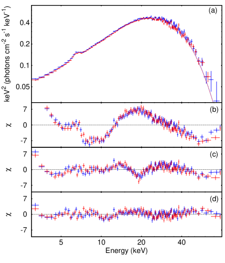
Fig. 3: Averaged energy spectrum of LMC X-4 and its best-fit approximation with the model III (a); deviations of the data from different approximation models: I (b), II (c) и III (d). Blue and magenta points correspond to the FPMA and FPMB modules, respectively.

Phase-averaged energy spectra

To approximate the spectrum of LMC X-4 we used several standard xspec models, commonly used to describe spectra of X-ray pulsars: (I) the power-law model with the exponential cutoff cutoffpl, (II) the power-law model with the high energy cutoff powerlaw $\times$ highecut (White et al. 1983) and (III) comptonization model comptt (Titarchuk 1994; Lyubarskii, Titarchuk 1995). To improve the quality of the approximation a component representing $K_{\alpha}$ iron line was added to each of models in the form of Gaussian (gaus xspec model). The interstellar absorption was also taken into account by adding the wabs component to the models. Thus, the final models used for the approximation of the LMC X-4 spectra can be written as:

Model I: wabs(cutoffpl + gaus)

Model II: wabs(powerlaw $\times$ highecut + gaus)

Model III: wabs(comptt + gaus)

Spectra for FPMA and FPMB modules data were analyzed simultaneously. In order to account the difference between the modules calibration a cross-calibration constant $C$ between them was included in all spectral models. The $\chi^{2}$ statistic was used to estimate the approximation quality. All models appeared to be insensitive to the value of the absorption, therefore in following it was fixed at $N_{\rm H}=5.74\times 10^{20}\text{ atoms cm}^{-2}$ (assuming Solar abundance). A gravitational redshift has been fixed for the model comptt on the value of $z=(1-2GM_{\ast}/R_{\ast}c^{2})^{-1/2}-1=0.3657$, estimated for the following parameters of the neutron star: $M_{\ast}=1.57M_{\hbox{$\odot$}}$ and $R_{\ast}=10^{6}\text{ cm}$. Best fit parameters for models I, II and III are presented in Table 1. The value of the a normalization coefficient was $C=1.021\pm 0.004$ for all the models.

Table 1: Parameters of the best approximation of the spectrum models of the LMC X-4

Parameter / Model	Model I	Model II	Model III
$N_{\rm H}(\times 10^{20}\text{ cm}^{-2})$	5.74	5.74	5.74
$T_{0}\text{ (keV)}$	…	…	0.56 $\pm$ 0.08
$kT\text{ (keV)}$	…	…	9.08 $\pm$ 0.04
$\tau$	…	…	14.15 $\pm$ 0.07
$\Gamma$	0.21 $\pm$ 0.01	0.834 $\pm$ 0.004	…
$E_{\rm cut}\text{ (keV)}$	…	19.35 $\pm$ 0.16	…
$E_{\rm fold}\text{ (keV)}$	14.11 $\pm$ 0.13	14.98 $\pm$ 0.18	…
$E_{\rm Fe}\text{ (keV)}$	6.43 $\pm$ 0.04	6.48 $\pm$ 0.03	6.46 $\pm$ 0.03
$\sigma_{\rm Fe}\text{ (keV)}$	0.11 $\pm$ 0.05	0.26 $\pm$ 0.03	0.41 $\pm$ 0.05
$EW_{\rm Fe}\text{ (eV)}$	41 $\pm$ 8	95 $\pm$ 7	158 $\pm$ 3
$\chi^{2}$ / d.o.f.	3.47 (2054)	1.27 (2053)	1.10 (2053)

Figure 3a shows the phase-averaged energy spectrum of LMC X-4 and its best-fit approximation with the model III. Deviations of the data from the approximation models I, II and III are shown in panels (b), (c) and (d), respectively. Both from the Table 1 and Figure 3 it can be clearly seen that the model III gives the best approximation with the value of $\chi^{2}=1.10$ for a 2053 degrees of freedom (d.o.f). The source flux in the energy range 3-79 keV is of $F_{\rm x}=(1.20\pm 0.05)\times 10^{-9}\text{ erg cm}^{-2}\text{ s}^{-1}$.

Phase-resolved spectroscopy

Pulse phase-resolved spectra of LMC X-4 were accounted in 16 uniformly distributed phase bins and approximated with the comptonization model III. Event list for each phase bin was created by selecting events in corresponding time intervals. This procedure was applied both for FPMA and FPMB data. We used the same approaches as for the phase-averaged spectra analysis for the approximation of the pulse phase-resolved spectra and estimate the quality of this approximation.

The $\chi^{2}$ (d.o.f.) value of the best-fit approximation of the pulse phase-resolved spectra varies from 0.88 to 1.12 for $\sim 1000$ degrees of freedom, that indicates an acceptable quality of the approximation. Figure 4 shows parameters of the model III as a function of the pulse phase in a comparison with the source pulse profile in the 3-10 and 10-20 keV energy ranges. It can be clearly seen that the characteristic temperature and the optical depth of the Compton emission are changed significantly with the pulse profile. The optical depth correlates with the pulse profile, while the maximum temperature is somewhat displaced in relation to the profile maximum.

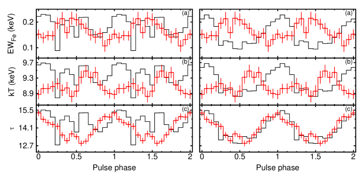
Fig. 4: Spectral parameters of the model III as a function of the pulse phase (red histograms) in a comparison with the source pulse profile in the 3-10 (left panel) and 10-20 keV (right panel) energy ranges.

At the same time, the behavior of the equivalent width of the iron line looks most interesting and demonstrates a significant phase shift in a comparison to the emission maximum. Based on the Fig. 4 we can estimate this phase shift as $\Delta\phi\sim 0.4$. Taking into account the source pulse period $P_{\rm spin}\simeq 13.5\text{ sec}$ the corresponding time delay is around $\Delta t\sim 5\text{ sec}$. This delay is likely to be related with the travel time of photons between the regions of their emission in the vicinity of the neutron star and the place where they are reflected. The distance which can be travelled by photons during $\sim 5$ seconds is about $\sim 1.5\times 10^{11}\text{ cm}$. Such a distance corresponds roughly to the outer radius of the accretion disk and is consistent with estimates presented by Neilsen et al. (2009) from the analysis of the Doppler broadening of the iron line.

Search for the cyclotron absorption line

To check the hypothesis of a possible presence of a cyclotron absorption line in the spectrum of the X-ray pulsar LMC X-4, the model III was modified by addition of the gabs component from the xspec package. Following the procedure applied by Tsygankov, Lutovinov (2005), the cyclotron line energy $E_{\rm cyc}$ was varied within the 5-55 keV energy range with the step of 3 keV. A corresponding line width $W$ was varied within 4-8 keV energy range with the step of 2 keV. For each pair of cyclotron line parameters the energy and the width were fixed in the gabs component and the resulting model was used to approximate the source spectrum. As a result, none of the combination of the line energy and its width does not result in a significant improvement of the fit and only the upper limit for the optical depth can be obtained.

Figure 5 shows the dependence for the upper limit for the optical depth of cyclotron line on the energy $E_{\rm cyc}$ for the three possible line widths: 4, 6 and 8 keV. The maximum value of the upper limit for the optical depth of the cyclotron line is $\sim 0.15$ ($3\sigma$). A similar search for the cyclotron absorption line in LMC X-4 was carried out for the pulse phase-resolved spectra. The corresponding upper limit on the optical depth is about $\sim 0.4$ ($3\sigma$).

Fig. 5: Dependence of the upper limit ($3\sigma$) on the optical depth of the cyclotron absorption line on the energy $E_{\rm cyc}$ for three different line width: 4 keV (solid line), 6 keV (dashed line) and 8 keV (dash-dotted line).

Power spectrum

Typically, the power spectrum of X-ray pulsars consists of the red noise component plus peaks at the pulsar spin frequency and its harmonics. According to the perturbation propagation model (Lyubarskii 1997; Churazov 2001), the red noise is generated in the accretion disk as a superposition of individual components arising at each specific radius at the corresponding characteristic diffuse timescale. The noise propagation inwards to the inner edge of the disk lead to the corresponding modulation of the accretion rate onto the compact object. The resulting power spectral density (PSD) has a form of a self-similar power-law up to the maximum frequency which can be generated in the disk (Hoshino, Takeshima 1993; Revnivtsev et al. 2009). In particular, Revnivtsev et al. (2009) showed that the power spectra of X-ray pulsars in the corotation contain a break at the frequency equal to the spin frequency of the neutron star (or in another words to the Keplerian frequency; $f_{\rm br}\approx\nu_{\rm k}$).

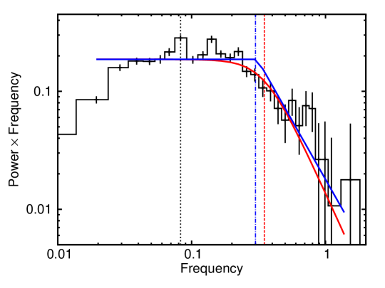
Fig. 6: Power spectral density of LMC X-4. Solid blue line represents the spectrum approximation with the model 1 ($\alpha_{2}=-2.0$, $f_{\rm br}=0.3$ Hz). Solid red line represents spectrum approximation with the model 2 ($\alpha=-2.5$, $f_{\rm br}=0.35$ Hz). Vertical lines show positions of the corresponding break frequency: $f_{\rm br}=0.3\text{ Hz}$ (dash-dotted line) and $f_{\rm br}=0.35\text{ Hz}$ (dashed line); and the position of the spin frequency (dotted line).

Figure 6 shows the power spectrum of LMC X-4 in the energy range 3-79 keV in units of the power multiplied by the frequency. Two models were used for the approximation:
a broken power-law model, the model 1:

$$P\propto\begin{cases}f^{\alpha_{1}},[f<f_{\rm br}]\\ f_{br}^{\alpha_{1}-\alpha_{2}}f^{\alpha_{2}},[f>f_{\rm br}]\end{cases},$$ (1)

where $\alpha_{1}$ и $\alpha_{2}$ – slopes of the power-law, $\alpha_{1}$ value was fixed at -1, $f_{\rm br}$ - break frequency;

and a model with a smooth transition between the two power-law functions (Revnivtsev et al. 2009), the model 2:

$$P\propto f^{-1}\times\left[1+\left(\dfrac{f}{f_{\rm br}}\right)^{4}\right]^{-\alpha/4},$$ (2)

where $f_{\rm br}$ – break frequency and $\alpha$ – the power-law index.

Results of the PSD approximation with both models are shown in Fig. 6. The solid blue line corresponds to the model 1 with the following parameters: the break frequency $f_{\rm br}\simeq 0.3\text{ Hz}$, the power-law index $\alpha_{2}=-2.0$. The solid red line shows the result of the approximation by the model 2 with the following parameters: the break frequency $f_{\rm br}\simeq 0.35\text{ Hz}$, the power-law index $\alpha=-2.5$.

X-ray tomography of the emitting regions

The NuSTAR observation covers approximately a half of the orbital cycle of the binary system ($\Psi_{\rm orb}\simeq[0.4;0.9]$). It makes possible to carry out a tomography of the areas where X-ray emission is generated. In particular, if the iron line Fe $\rm K_{\alpha}$ is generated due to reflection of the original emission in certain areas (regions) of the binary system, then observing the system at different angles (in different orbital phases), one can attempt to locate these regions and their geometry. The energy resolution of the NuSTAR observatory doesn’t allow to carry out a detailed Doppler imaging of the object. Therefore we confine ourselves by a rough approximation, which allow us to get qualitative estimates on time delay in the system.

Using the Chandra and XMM-Newton observations Neilsen et al. (2009) carried out the analysis of regions of the formation of the lines in the spectrum of LMC X-4. These authors found that changes in the intensity and width of spectral lines of different elements depend on the phase of superorbital motion. They also proposed three possible areas of the lines generation in the binary system: the photoionized stellar wind region, the outer region of the standard accretion disk and the inner region of the curved accretion disk. According to the assumptions of Neilsen et al. (2009) the most probable area of the formation of the Fe $\rm K_{\alpha}$ line is the outer edge of the accretion disk and/or the inflow accretion stream, which falls on the outer edge of the disk through the inner Lagrange point. If the Fe $\rm K_{\alpha}$ line is generated due to the irradiation of the pulsar emission at the outer edge of the accretion disk or at the inflow stream, one can expect a correlation between the pulse profile and the line parameters (e.g., equivalent width). Moreover, this correlation will look different for different orbital phases, depending on the place where the line is formed – at the outer edge of the accretion disk or in the place where inflow accretion stream touches the outer edge of the disk (the so-called hot spot, see Armitrage, Livio 1996 and references therein).

Table 2: Parameters of the LMC X-4 spectra in different orbital phases.

Parameter / Phase	$\Psi_{\rm orb}^{(1)}$	$\Psi_{\rm orb}^{(2)}$	$\Psi_{\rm orb}^{(3)}$
$C$	$1.021\pm 0.006$	$1.016\pm 0.006$	$1.034\pm 0.006$
$N_{\rm H}(\times 10^{20}\text{ cm}^{-2})$	5.74	5.74	5.74
$T_{0}\text{ (keV)}$	0.56	0.56	0.56
$kT\text{ (keV)}$	9.03 $\pm$ 0.06	9.10 $\pm$ 0.06	8.99 $\pm$ 0.06
$\tau$	13.91 $\pm$ 0.10	13.94 $\pm$ 0.10	14.3 $\pm$ 0.11
$E_{\rm Fe}\text{ (keV)}$	6.49 $\pm$ 0.05	6.53 $\pm$ 0.06	6.38 $\pm$ 0.07
$\sigma_{\rm Fe}\text{ (keV)}$	0.34 $\pm$ 0.09	0.35 $\pm$ 0.07	0.54 $\pm$ 0.09
$EW_{\rm Fe}\text{ (eV)}$	140 $\pm$ 10	142 $\pm$ 11	218 $\pm$ 15
$\chi^{2}$ / d.o.f.	1.05 (1531)	1.01 (1528)	1.07 (1529)

Indeed, for the superorbital phase $\Psi_{\rm sup}\sim 0$ the plane of the accretion disk is positioned in the direction to the observer at an angle close to the normal. If the iron line is generated at the outer edge of the accretion disk, we will observe a constant phase shift between the maximum of its equivalent width and the maximum of the pulse profile during the binary motion of the neutron star. If the Fe $\rm K_{\alpha}$ line is produced in the inflow stream (hot spot), one can expect variations in the phase shift or in the width profile, depending on the orbital phase. This is because the system asymmetry in relation to the distant observer, defined by the presence of the hot spot or the inflow stream on the disk edge. To check this assumptions, the entire observation was divided into three equal subintervals (orbital phases: $\Psi_{\rm orb}^{(1)}\simeq[0.40-0.56]$, $\Psi_{\rm orb}^{(2)}\simeq[0.56-0.72]$ и $\Psi_{\rm orb}^{(3)}\simeq[0.72-0.90]$). Both phase-averaged and pulse phase-resolved spectra were produced in every subinterval. As before, they all were approximated by the comptonization model III.

The best fit parameters of the pulse-averaged spectra for each of the three orbital phases are presented in Table 2. The temperature of the seed photons $T_{0}$ is restricted poorly due to lack of statistics, therefore it was fixed at $T_{0}=0.56\text{ keV}$, measured for the total spectrum (see Table 1). It can be seen from the Table 2 that for all the three orbital phases the spectral parameters coincide to each other within the uncertainties, except the iron line equivalent width. In the third orbital phase interval ($\Psi_{\rm orb}^{(3)}$) the equivalent width of the line of iron ($EW_{\rm Fe}$) by factor of $\sim 1.5$ higher than in the first and second phase intervals.

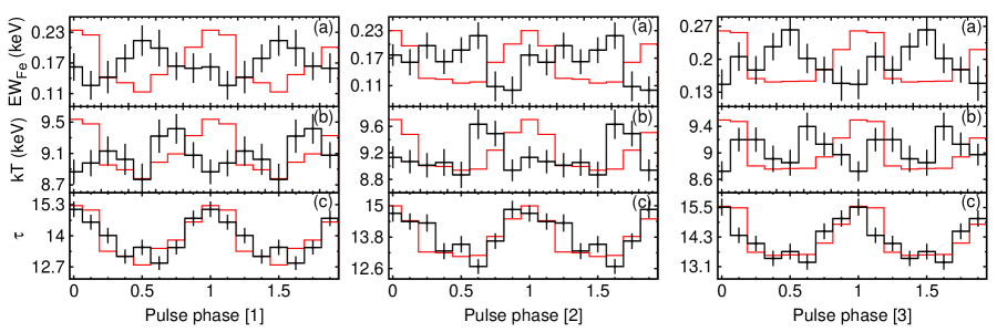
Fig. 7: Dependence of the spectral parameters of LMC X-4 on the pulse phase for different orbital phases $\Psi_{\rm orb}^{(1)}$, $\Psi_{\rm orb}^{(2)}$ and $\Psi_{\rm orb}^{(3)}$ (red histograms). The black line in each panel shows the corresponding pulse profile in a 10-20 keV energy range.

Figure 7 shows variations of the spectral parameters with the pulse phase for each of the three orbital intervals in a comparison with corresponding source pulse profile in the 10-20 keV energy range. One can be seen that at orbital phases $\Psi_{\rm orb}^{(1)}$ and $\Psi_{\rm or}^{(3)}$ an anti-correlation between the pulse profile and the equivalent width of Fe $\rm K_{\alpha}$ is observed. Moreover, the shape of the equivalent width changes at these phases has a pronounced maximum and minimum shifted about the half of the pulse phase. At the same time at the orbital phases $\Psi_{\rm orb}^{(2)}$ the shape of the equivalent width becomes asymmetric and its maximum shifts by $\sim 0.1$ of the pulse phase. Thus, results of the pulse phase-resolved spectroscopy demonstrates clearly variations in the phase shift and in the width profile depending on the orbital motion of the pulsar. For the better clarity all the three profiles of the equivalent line width Fe $\rm K_{\alpha}$ is presented in-line in Fig. 8.

Fig. 8: Dependence of the equivalent width of the iron line on the pulse phase in different orbital phases $\Psi_{\rm orb}^{(1)}$ (a), $\Psi_{\rm orb}^{(2)}$ (b) and $\Psi_{\rm orb}^{(3)}$ (c). See text for details.

Based on these results one can assume that the generation of the Fe $\rm K_{\alpha}$ line occurs in the inflowing stream or in the area of the interaction between the stream and the outer edge of the accretion disk. It should be noticed that the interaction between the stream and the accretion disk is quite complex and depends on a large number of parameters of the binary system and peculiarities of the matter transfer between the components (see, e.g., Bisikalo et al. 2013). In particular, the hot spot itself doesn’t always appear in the place of the interaction of the inflowing stream and the accretion disk. Therefore, additional observations, involving data from other observatories, are needed for the detailed analysis and obtaining the quantitative parameters of the Fe $\rm K_{\alpha}$ line generation area.

CONCLUSION

In this paper, using the NuSTAR observatory data, the broadband spectrum of the X-ray pulsar LMC X-4 was obtained in the energy range $3-79\text{ keV}$ with the high statistical significance and good energy resolution. It allowed us to test several spectral models and to determine their parameters. It was shown that the obtained spectrum can be approximated in the best way by the comptonization model (comptt) with the inclusion of the interstellar absorption and the $K_{\alpha}$ iron line. The equivalent width of the iron line in the averaged spectrum was of $EW_{\rm Fe}\simeq 158\text{ eV}$.

We searched for the cyclotron absorption line in the source averaged spectrum in the energy range $5-55\text{ keV}$ and for different possible equivalent line width (2-8 keV). The resulting upper limit on its optical depth $\simeq 0.15$ ($3\sigma$) indicates the absence of the cyclotron feature in a given energy range. This allows us to put a limit on the possible magnitude of the magnetic field on the surface of the neutron star in LMC X-4: $B<3\times 10^{11}\text{ G}$ or $B>6.5\times 10^{12}\text{ G}$. Search for the cyclotron absorption line was also carried out for pulse phase-resolved spectra and also showed the absence of the cyclotron feature in the energy range mentioned above.

The pulse phase-resolved spectroscopy was carried out for LMC X-4 for the first time in the wide energy band with the good spectral resolution. The phase-resolved spectra were approximated by the same comptonization model as the averaged one. The comparison of the behavior of the spectral parameters with the pulse profile at the energies above 10 keV has shown a correlation of the source intensity with the Compton optical depth and anti-correlation with the temperature and the equivalent width of the iron line. We determined the delay ($\sim 5\text{ sec}$) between the peaks of the source emission and the equivalent width of the iron line, apparently associated with the travel time of photons between the emitting regions in the vicinity of the neutron star and the relatively cold regions where this emission is reflected (presumably, at the inflowing stream or at the place of an interaction of the stream and the outer edge of the accretion disk). The tomography analysis of the Fe $\rm K_{\alpha}$ line implies that this emission originates not just on the outer edge of the accretion disk, but most likely in the inflowing accretion stream or in the area where this flow interacts with the outer edge of the accretion disk (the so-called hot spot). However this assumption requires more detailed study. It is also worth noticing that in the energy range of 3–10 keV, where the pulse profile has a more complex shape, there were no clear correlation between the model parameters and the observed pulse profile.

The tomography of the emitting areas allows us to suggest that the generation of the Fe $\rm K_{\alpha}$ line, emerging as a result of the reflection of the original X-ray flux in relatively cold areas of the surrounding matter, is not just on the outer edge of the accretion disk, but most likely in the inflowing stream that flows through inner Lagrangian point and falls on the outer accretion disk edge or in the area where flow interacts outer edge of the accretion disk (the so-called hot spot).

However this assumption requires more detailed study. It is also worth noticing that in in energy range of 3–10 keV, where the pulse profile has a more complex shape, there were no clear correlation between the model parameters and the form of profile of the pulse observed.

Revnivtsev et al. (2009) and Tsygankov et al. (2012) demonstrated the possibility of using the noise power spectral density shape to determine the magnetic field strength of the neutron star in X-ray pulsars. This method is based on the equality of the break frequency in the PSD and the Keplerian frequency on the inner edge of the accretion disk ($f_{\rm br}\approx\nu_{\rm k}$; Revnivtsev et al 2009).

Substituting in the expression for the Keplerian motion the mass of the neutron star in LMC X-4 $M_{\ast}=1.57M_{\hbox{$\odot$}}$ and the break frequency, measured from the PSD $f_{\rm br}\simeq(0.30-0.35)\text{ Hz}$, we can estimate the magnetospheric radius as $R_{\rm m}\sim(3.5-3.9)\times 10^{8}\text{ cm}$. The radius of the magnetosphere, in turn, is determined by the strength of the magnetic field of the neutron star (see, e.g., Tsygankov et al., 2016):

$$R_{\rm m}=\xi\dot{M}^{-2/7}\mu^{4/7}(2GM)^{-1/7},$$ (3)

where $\xi$ – dimensionless coefficient, taking into account non-spherical nature of accretion ($\xi\sim 0.5$; Long et al. 2005; Parfrey et al. 2015), $\mu$ – magnetic moment of the neutron star and $\dot{M}$ – mass accretion rate.

The flux measured from the pulsar in the 3-79 keV energy band is $F_{\rm x}\sim 1.20\times 10^{-9}\text{erg cm}^{-2}\text{sec}^{-1}$ which can be roughly considered as a bolometric one (the flux in the 0.5-100 keV energy range is $F_{\rm x}\sim 1.22\times 10^{-9}\text{erg cm}^{-2}\text{sec}^{-1}$). This corresponds to the bolometric luminosity of the source $L_{\rm x}\sim 3.6\times 10^{38}\text{ erg sec}^{-1}$ and the mass accretion rate $\dot{M}\sim 6.3\times 10^{-8}M_{\hbox{$\odot$}}\text{ year}^{-1}$. By making the Keplerian radius equal to the magnetospheric radius we can estimate the magnetic field strength of the neutron star in LMC X-4: $B\simeq(2.7-3.2)\times 10^{13}\text{ G}$, which can be roughly translated to the energy of the possible cyclotron line $230-270\text{ keV}$. Formally, this value is agreed with the lower limit obtained from the analysis of the energy spectrum of the pulsar.

REFERENCES

Armitage, Livio (P. Armitage, M. Livio), Astrophys. J. 470, 1024 (1996).
Bisikalo et al. (D. V. Bisikalo, A. G. Zhilkin, A. A. Boyuarchuk), ”Gas dynamics in the dense binary stars”, M.: Fizmatlit (2013).
Boldin et al. (P. A. Boldin, S. S. Tsygankov, A. A. Lutovinov), Astron. Lett. 39, 375 (2013).
Churazov et al. (E. Churazov, M. Gilfanov, M. Revnivtsev) Mon. Not. Roy. Astron. Soc. 321, 759 (2001).
Chevalier, Ilovaisky, (C. Chevalier, S. A. Ilovaisky) Astron. Astrophys. 59, L9 (1977).
Epsteinet al. (A. Epstein, J. Delvaille, H. Helmken, S. Murray, H. W. Schnopper, R. Doxsey, F. Primini) Astrophys. J. 216, 103 (1977).
Giacconi et al. (R. Giacconi, S. Murray, H. Gursky, E. Kellogg, E. Schreier, H. Tananbaum), Astrophys. J. 178, 281 (1972).
Ghosh, Lamb (P. Ghosh, F. K. Lamb) Astrophys. J. 234, 296 (1979).
Grebenev et al. (S. Grebenev, A. Lutovinov, S. Tsygankov, I. Mereminskiy), Mon. Not. Roy. Astron. Soc. 428, 50 (2013).
Kelley et al. (R. L. Kelley, J. G. Jernigan, A. Levine, L. D. Petro, S. Rappaport) Astrophys. J. 264, 568 (1983).
Krivonos et al. (R. A. Krivonos et al.) Astrophys. J. 809, 140 (2015).
La Barbera et al. (A. La Barbera, L. Burderi, T. Di Salvo, R. Iaria, N. R. Robba) Astrophys. J. 553, 375 (2001).
Lamb et al. (F. K. Lamb, C. J. Pethick, D. Pines), Astrophys. J. 184, 271 (1972).
Lang et al. (F. L. Lang et al.) Astrophys. J. 246, L21 (1981).
Levine et al. (A. Levine, S. Rappaport, A. Putney, R. Corbet, F. Nagase) Astrophys. J. 381, 101 (1991).
Levine et al. (A. M. Levine, S. A. Rappaport, G. Zojcheski) Astrophys. J. 541, 194 (2000).
Li et al. (F. Li, S. Rappaport, A. Epstein) Nature 271, 37 (1978).
Long et al. (M. Long, M. M. Romanova, R. V. E Lovelace) Astrophys. J. 764, 196 (2005).
Lutovinov, Tsygankov ((A. A. Lutovinov, S. S. Tsygankov), Astron. Lett. 35, 433 (2009).
Lyubarskii (Y. E. Lyubarskii) Mon. Not. Roy. Astron. Soc. 292, 679 (1997).
Molkov et al. (S. Molkov, A. Lutovinov, M. Falanga), Astron. Lett. 41, 562 (2015).
Molkov et al. (S. Molkov, A. Lutovinov, M. Falanga, S. Tsygankov, E.Bozzo) Mon. Not. Roy. Astron. Soc., accepted (2016).
Moon et al. (D.-S. Moon, S. S. Eikenberry) Astrophys. J. 549, L225 (2001).
Mushtukov et al. (A. Mushtukov, V. Suleimanov, S. Tsygankov, J. Poutanen) Mon. Not. Roy. Astron. Soc. 454, 2539 (2015).
Nagase (F. Nagase) Publ. Astron. Soc. Japan 41, 1 (1989).
Naranan et al. (S. Naranan, R. F. Elsner, W. Darbro, B. D. Ramsey, D. A. Leahy, M. C. Weisskopf) Astrophys. J. 290, 487 (1985).
Neilsen et al. (J. Neilsen, J. C. Lee, M. A. Nowak, K. Dennerl, S. D. Vrtilek) Astrophys. J. 696, 182 (2009).
Parfrey et al. (K. Parfrey, A. Spitkovsky, A. M. Beloborodov) Astrophys. J. 822, 33 (2016).
Revnivtsev et al. (M. Revnivtsev, E. Churazov, K. Postnov, S. Tsygankov) Astron. Astrophys. 507, 1211 (2009).
Titarchuk (L. Titarchuk) Astrophys. J. 434, 570 (1994).
Titarchuk, Lyubarskij (L. Titarchuk, Yu. Lyubarskij) Astrophys. J. 450, 876 (1995).
Falanga et al. (M. Falanga, E. Bozzo, A. Lutovinov, J. M. Bonnet-Bidaud, Y. Fetisova, J. Puls) Astron. Astrophys. 577, A310 (2015).
Harrison et al. (F. A. Harrison et al.) Astrophys. J. 770, 103 (2013)
Hickox et al. (R. C. Hickox, R. Narayan and T. R. Kallman) Astrophys. J. 614, 881 (2004).
Heemskerk, van Paradijs (M. H. M. Heemskerk, J. van Paradijs) Astron. Astrophys. 223, 154 (1985).
Hoshino, Takeshima (M. Hoshino, T. Takeshima) Astrophys. J. 411, L79 (1993).
Tsygankov, Lutovinov (S. S. Tsygankov, A. A. Lutovinov), Astron. Lett. 31, 380 (2005).
Tsygankov et al. (S. S. Tsygankov, R. A. Krivonos, A. A. Lutovinov) Mon. Not. Roy. Astron. Soc. 421, 2407 (2012).
Tsygankov et al. (S. S. Tsygankov, A. A. Mushtukov, V. F. Suleimanov, J. Poutanen) Mon. Not. Roy. Astron. Soc. 457, 1101 (2016).
Walter et al. (R. Walter, A. A. Lutovinov, E. Bozzo, S. S. Tsygankov), Astron. Astrophys. Rev. 23, id. 2 (2015).
White (N. E. White) Nature 271, 38 (1978).
White et al. (N. E. White, J. H. Swank, S. S. Holt) Astrophys. J. 270, 711 (1983).
Woo et al. (J. W. Woo, G. W. Clark, A. M. Levine, R. H. D. Corbet, F. Nagase) Astrophys. J. 467, 811 (1996).