Dis-S2V: Discourse Informed Sen2Vec

Abstract

Vector representation of sentences is important for many text processing tasks that involve clustering, classifying, or ranking sentences. Recently, distributed representation of sentences learned by neural models from unlabeled data has been shown to outperform the traditional bag-of-words representation. However, most of these learning methods consider only the content of a sentence and disregard the relations among sentences in a discourse by and large.

In this paper, we propose a series of novel models for learning latent representations of sentences (Sen2Vec) that consider the content of a sentence as well as inter-sentence relations. We first represent the inter-sentence relations with a language network and then use the network to induce contextual information into the content-based Sen2Vec models. Two different approaches are introduced to exploit the information in the network. Our first approach retrofits (already trained) Sen2Vec vectors with respect to the network in two different ways: (i) using the adjacency relations of a node, and (ii) using a stochastic sampling method which is more flexible in sampling neighbors of a node. The second approach uses a regularizer to encode the information in the network into the existing Sen2Vec model. Experimental results show that our proposed models outperform existing methods in three fundamental information system tasks demonstrating the effectiveness of our approach. The models leverage the computational power of multi-core CPUs to achieve fine-grained computational efficiency. We make our code publicly available upon acceptance.

<concept> <concept_id>10010147.10010257.10010293.10010319</concept_id> <concept_desc>Computing methodologies Learning latent representations</concept_desc> <concept_significance>500</concept_significance> </concept> <ccs2012> <concept> <concept_id>10002951.10003317.10003347.10003356</concept_id> <concept_desc>Information systems Clustering and classification</concept_desc> <concept_significance>500</concept_significance> </concept> <concept> <concept_id>10002951.10003317.10003347.10003357</concept_id> <concept_desc>Information systems Summarization</concept_desc> <concept_significance>500</concept_significance> </concept>

</ccs2012> [500]Computing methodologies Learning latent representations [500]Information systems Clustering and classification [500]Information systems Summarization

1 Introduction and Motivation

Many sentence-level text processing tasks rely on representing the sentences using fixed-length vectors. For example, classifying sentences into topics using a statistical classifier like Maximum Entropy would require the sentences to be represented by vectors. Similarly, for the task of ranking sentences based on their importance in the text using a ranking model like LexRank [3] or SVMRank [9], one needs to first represent the sentences with fixed-length vectors. The most common method uses a bag-of-words or a bag-of-ngrams representation, where each dimension of the vector is computed by some form of term frequency statistics (e.g., tf*idf).

Recently, distributed representations, in the form of dense real-valued vectors, learned by neural network models from unlabeled data, has been shown to outperform the traditional bag-of-words representation [12]. Distributed representations encode the semantics of linguistic units and yield better generalization [15, 2]. However, most existing methods to devise distributed representation for sentences consider only the content of a sentence, and disregard relations between sentences in a text by and large [12, 6]. But, sentences rarely stand of their own in a well-written text. On a finer level, sentences are connected with each other by certain logical relations (e.g., elaboration, contrast) to express the meaning as a whole [8]. On a coarser level, sentences in a text address a common topic, often covering multiple subtopics; i.e., sentences are also topically related [22]. Our main hypothesis in this paper is that distributed representation methods for sentences should not only consider the content of the sentence but also the inter-sentence relations.

Recent work on learning distributed representations for words has shown that semantic relations between words (e.g., synonymy, hypernymy, hyponymy) encoded in semantic lexicons like WordNet [16] or Framenet [1] can improve the quality of word vectors that are trained solely on unlabeled data [27, 4, 28]. Our work in this paper is reminiscent of this line of research with a couple of crucial differences. Firstly, we are interested in representation of sentences as opposed to words, for which such resources are not readily available. Secondly, our main goal is to incorporate discourse information in the form of inter-sentence relations as opposed to semantic relations between words. These differences posit a number of new research challenges: (i) how can we represent inter-sentence relations? (ii) how can we effectively exploit the inter-sentence relations in our representation learning model? and (iii) how can we evaluate our model?

In this paper, we propose novel models for learning distributed representations for sentences that consider not only content of a sentence but relations among sentences. We represent inter-sentence relations using a network, where nodes represent sentences and edges represent similarity between the corresponding sentences. Our choice of network to represent inter-sentence relations is due to the facts that networks provide flexible ways to represent relations between any pair of sentences, and recent advances in learning distributed representations for nodes and edges in networks have shown promising results [5, 25, 24, 19].

We explore two different approaches to exploit the information in the network. In our first approach, we learn sentence vectors using existing content-based models, i.e., the Sen2Vec model proposed in [12]. Then we retrofit these vectors using information encoded in network to encourage the new vectors to be similar to the vectors of related sentences and similar to their prior representations. The retrofitting is performed in two different ways: (i) by using an efficient iterative algorithm [23, 4] that incorporates adjacency relations in $1$-hop neighborhood of a node, and (ii) by training a discriminative model that seeks to preserve local neighborhoods of nodes, and in such case, the neighborhood is sampled by a flexible stochastic sampling method [5]. In our second approach, we alter the objective function of the original Sen2Vec model with a regularizer or prior that encourages related sentences in the network to have similar vector representations. Therefore, in this approach the vectors are learned from scratch by jointly modeling the content of the sentences and the relations between sentences.

Different approaches to evaluate sentence representation methods have been proposed including sentence-level prediction tasks (e.g., sentiment classification, paraphrase identification) and sentence-pair similarity computation task [6, 12]. Since existing representation methods encode vectors for each sentence independently, these evaluation methodologies are trivial. In contrast, our learning methods exploit inter-sentence similarities, which can be constrained by document boundaries. Therefore, we require datasets containing documents with sentence-level annotations.

We evaluate our models on three different types of tasks: classification, clustering and ranking. In particular, we consider the tasks of classifying and clustering sentences into topics, and of ranking sentences in a document to create an extractive summary of the document (i.e., by selecting the top-ranked sentences). There are standard datasets with document-level topic annotations (e.g., Reuters-21578, 20 Newsgroups). However, to our knowledge, no dataset exists with topic annotations at the sentence level. We generate sentence-level topic annotations from the document-level ones by selecting subsets of sentences that can be considered as representatives of the document and label them with the same document-level topic label. We use the standard DUC 2001 and 2002 datasets to evaluate our models on the summarization task, where we compare the system-generated summaries with the human-authored summaries.

Our experimental results on these tasks demonstrate that the models which induce information encoded in the discourse network in the form of inter-sentence relations during learning (i.e., the regularized models) consistently outperform the content-only baseline by a good margin in all tasks, whereas the retrofitted models perform comparatively better on the classification and on the clustering tasks.

2 Methodology

Let $G=(V,E,W)$ be a discourse graph, where a node $\mathbf{v}\in V$ represents a sentence and the edge weight $w(\mathbf{u},\mathbf{v})\in W$ reflects some form of similarity between sentences $\mathbf{u}$ and $\mathbf{v}$. A sentence $\mathbf{v}$ is a sequence of words $(v_{1},v_{2}\cdots v_{m})$, each coming from a vocabulary $\Omega$, i.e., $v_{i}\in\Omega$. We define $N(\mathbf{v})$ as the set of neighbors of a sentence $\mathbf{v}$ in $G$. Let $\phi:V\rightarrow\operatorname{\mathbb{R}}^{d}$ be the mapping function from sentences to their distributed representations, i.e., real-valued vectors of $d$ dimensions. Our goal is to learn $\phi$ by exploiting information from two different sources: (i) the content of the sentence, $\mathbf{v}=(v_{1},v_{2}\cdots v_{m})$; and (ii) the neighborhood of the sentence, $N(\mathbf{v})$.

In the following, we first describe how we construct the discourse graph $G$ for our problem (Section 2.1). We then briefly describe existing sentence representation methods that consider only the sentence contents (Section 2.2). In Section 2.3, we demonstrate a network-based representation method that considers only the neighborhood information. Finally, we present our retrofitting (Section 2.4) and regularized methods (Section 2.5) that incorporate both content and network neighborhood information into a single model.

2.1 Discourse Graph Formulation

Let $D=\{\mathbf{v}_{1},\mathbf{v}_{2},\cdots,\mathbf{v}_{n}\}$ be the set of sentences in our dataset, which constitutes the nodes in the discourse graph. The edge weights $w(\mathbf{v}_{i},\mathbf{v}_{j})$ are computed by measuring the similarity between the corresponding sentences, $\sigma(\mathbf{v}_{i},\mathbf{v}_{j})$. Here $\sigma$ denotes a similarity metric (e.g., Cosine, Jaccard).

For constructing the network, we distinguish between two types of edges: (i) intra-document edges, i.e., edges between sentences of the same document, and (ii) across-document edges, i.e., edges between sentences of different documents. Different thresholding parameters can be set depending on whether the edges are intra–document or across-documents.

2.2 Content-based Model (S2V)

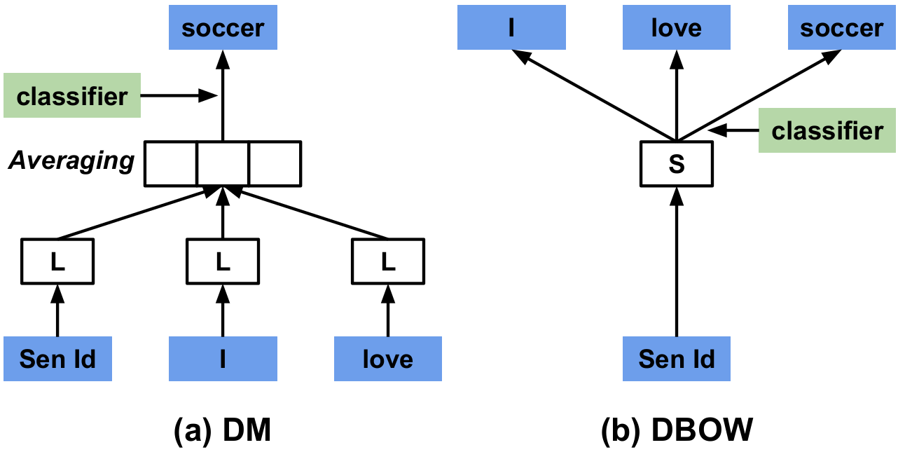
Figure 1: Distributed memory (DM) and Distributed bag of words (DBOW) versions of Sen2Vec.

We use the Sen2Vec model proposed in [12] as our baseline model, which is trained solely based on the contents of the sentences. This approach concatenates the vectors learned by the two models shown in Figure 1: (a) a distributed memory (DM) model, and (b) a distributed bag of words (DBOW) model. In the DM model, every sentence in the dataset $D$ is represented by a $d$ dimensional vector in a shared lookup matrix $S\in\operatorname{\mathbb{R}}^{n\times d}$. Similarly, every word in the vocabulary $\Omega$ is represented by a $d$ dimensional vector in another shared lookup matrix $L\in\operatorname{\mathbb{R}}^{|\Omega|\times d}$. Given an input sentence $\mathbf{v}=(v_{1},v_{2}\cdots v_{m})$, the corresponding sentence vector from $S$ and the corresponding word vectors from $L$ are averaged to predict the next word in a context. More formally, let $\phi$ denote the mapping from sentence and word ids to their respective vectors in $S$ and $L$, the DM model minimizes the following objective (negative log likelihood):

$$J(\phi) = -\sum_{t=k}^{m-k}\log P(v_{t}|\mathbf{v};v_{t-k+1},\cdots,v_{t-1})$$ (1)

$$= -\sum_{t=k}^{m-k}\log\frac{\exp(\omega(v_{t})^{T}\mathbf{z})}{\sum_{i}\exp(\omega(v_{i})^{T}\mathbf{z})}$$ (2)

where $\mathbf{z}$ is the average of $\phi(\mathbf{v}),\phi(v_{t-k+1}),\cdots,\phi(v_{t-1})$ input vectors, and $\omega(v_{t})$ is the output vector representation of word $v_{t}\in\Omega$. The sentence vector $\phi(\mathbf{v})$ is shared across all (sliding window) contexts extracted from the same sentence, thus acts as a distributed memory.

In stead of predicting the next word in the context, the DBOW model predicts the words in the context independently given the sentence id as input. More formally, DBOW minimizes the following negative log likelihood objective:

$$J(\phi) = -\sum_{t=k}^{m-k}\sum_{j=t-k+1}^{t}\log P(v_{j}|\mathbf{v})$$ (3)

$$= -\sum_{t=k}^{m-k}\sum_{j=t-k+1}^{t}\log\frac{\exp(\omega(v_{j})^{T}\phi(\mathbf{v}))}{\sum_{i}\exp(\omega(v_{i})^{T}\phi(\mathbf{v}))}$$ (4)

2.3 Network-based Model (N2V)

The network-based representation model considers only the neighborhood information of the nodes. We use the recently proposed Node2Vec method [5]. It uses the skip-gram model of Word2Vec [14] with the intuition that nodes within a graph context (or neighborhood) should have similar representations. The negative log likelihood objective of the skip-gram model for graphs can be defined as:

$$J(\phi) = -\sum_{\mathbf{v}\in V}\log P(N(\mathbf{v})|\phi(\mathbf{v}))$$ (5)

$$= -\sum_{\mathbf{v}\in V}\sum_{\mathbf{n}_{i}\in N(\mathbf{v})}\log P(\mathbf{n}_{i}|\phi(\mathbf{v}))$$ (6)

$$= -\sum_{\mathbf{v}\in V}\sum_{\mathbf{n}_{i}\in N(\mathbf{v})}\log\frac{\exp(\omega(\mathbf{n}_{i})^{T}\phi(\mathbf{v}))}{\sum_{\mathbf{x}\in V}\exp(\omega(\mathbf{x})^{T}\phi(\mathbf{v}))}$$ (7)

where as before, $\phi$ and $\omega$ denote the input and the output vector representations of the nodes (sentences). The neighboring nodes $N(\mathbf{v})$ forms the context for node $\mathbf{v}$. Node2Vec uses a biased random walk which adaptively combines breadth first search (BFS) and depth first search (DFS) to find the neighborhood of a node. The walk attempts to capture two properties of a graph often used for prediction tasks in networks: (i) homophily and (ii) structural equivalence. According to homophily, nodes in the same group or community should have similar representations (e.g., sentences in a topic). Structural equivalence suggests that nodes with similar structural roles (hub, bridge) should have similar representations (e.g., central sentences). In a real-world network, nodes exhibit mixed properties.

Figure 2: Random walk for generating samples.

The controlled random walk in Node2Vec interpolates between BFS and DFS to generate multiple samples of $N(\mathbf{v})$ for each source node $\mathbf{v}$. Let $\mathbf{u}$ be a node just traversed from $\mathbf{p}$ (Figure 2) in a random walk that started from a source node $\mathbf{v}$. The walk is controlled by (unnormalized) transition probabilities $\tau_{u,x}=\mu_{r,f}(\mathbf{p},\mathbf{x}).w_{v,x}$, where

$$\mu_{r,f}(\mathbf{p},\mathbf{x})=\begin{cases}\frac{1}{r},&\text{if}\ \delta_{p,x}=0\\ 1,&\text{if}\ \delta_{p,x}=1\\ \frac{1}{f}&\text{if}\ \delta_{p,x}=2\\ \end{cases}$$ (8)

where $\delta_{p,x}$ is the distance from node $\mathbf{p}$ to $\mathbf{x}$. The return parameter $r$ controls the likelihood of revisiting a node; large value will reduce duplicate samples and small value will keep the search local. The forward parameter $f$ controls the distance covered by the walk; for $f>1$, the walk will act as BFS and for $f<1$, it will act as DFS. Given a graph, we can precompute $\tau$ by keeping three possible values corresponding to Equation 8 for each edge transition.

We can apply Node2Vec directly to the discourse graph to learn vector representations for the sentences. This adaptation of the model considers only inter-sentence relations defined by the graph. Since the graph in our case is formed by matching the contents of the sentences, this method indirectly takes contents of individual sentences into account.

In order to incorporate contents directly, we could have a variant of the Node2Vec model, where in stead of randomly initializing the vectors, we initialize them with the precomputed vectors from the content-based model described in Section 2.2. However, we hypothesize that a more effective approach is to consider both sources of information simultaneously in a controllable joint framework.

2.4 Dis-S2V by Retrofitting

We explore the general idea of retrofitting [4] to incorporate information from both the content and the neighborhood of a node (or a sentence) in a joint learning framework. Let $\phi^{\prime}(\mathbf{v})$ denote the vector representation for sentence $\mathbf{v}$ that has already been learned by our content-based method in Section 2.2. Our aim is to retrofit this vector on the discourse graph $G$ such that the revised vector $\phi(\mathbf{v})$: (i) is also similar to the prior vector $\phi^{\prime}(\mathbf{v})$, and (ii) is similar to the vectors of its adjacent nodes $\phi(\mathbf{u})$. To this end, we define the following objective function to minimize:

Input : 
- Graph $G=(V,E,W)$
- Prior vectors $\phi^{\prime}$
- Probabilities $\alpha_{v}$ and $\beta_{v}$ for all $\mathbf{v}\in V$

Output : Retrofitted vectors $\phi$

1. $\phi\leftarrow\phi^{\prime}$ // initialization

2. repeat

         for all $\mathbf{v}\in V$ do

             $\phi(\mathbf{v})\leftarrow\frac{\alpha_{v}\phi^{\prime}(\mathbf{v})+\sum_{u}\left(\beta_{v}W_{v,u}+\beta_{u}W_{u,v}\right)\phi(\mathbf{u})}{\alpha_{v}+\sum_{u}\left(\beta_{v}W_{v,u}+\beta_{u}W_{u,v}\right)}$

            

       end for

      

until convergence;

Algorithm 1 Jacobi method for retrofitting.

$$J(\phi)=\sum_{\mathbf{v}\in V}\alpha_{v}||\phi(\mathbf{v})-\phi^{\prime}(\mathbf{v})||^{2}+\sum_{(u,v)\in E}\beta_{v}W_{u,v}||\phi(\mathbf{u})-\phi(\mathbf{v})||^{2}$$ (9)

where $\alpha$ values control the strength to which the algorithm should match the prior vectors, and $\beta$ values control the degree of smoothness based on the graph similarity. The quadratic cost in Equation 9 is convex in $\phi$, and has a closed form solution [23]. The closed form expression requires an inversion operation, which could be expensive for big graphs. A more efficient way is to use the Jacobi method, an online algorithm to solve the Equation iteratively. Algorithm 1 gives a pseudocode, which has the following update:

$$\phi(\mathbf{v})\leftarrow\frac{\alpha_{v}\phi^{\prime}(\mathbf{v})+\sum_{u}\left(\beta_{v}W_{v,u}+\beta_{u}W_{u,v}\right)\phi(\mathbf{u})}{\alpha_{v}+\sum_{u}\left(\beta_{v}W_{v,u}+\beta_{u}W_{u,v}\right)}$$ (10)

If for all $\mathbf{v}$$\in$$V$, $\alpha_{v}$$=$$\alpha$ and $\beta_{v}$$=$$\beta$, Equation 10 simplifies to:

$$\phi(\mathbf{v})\leftarrow\frac{\alpha\phi^{\prime}(\mathbf{v})+\sum_{u}W_{u,v}~{}\phi(\mathbf{u})}{\alpha+\sum_{u}W_{u,v}}$$ (11)

We can show a correspondence between this method and a biased random walk over $G$, where at any vertex $\mathbf{v}\in V$, the walk faces two options: (i) with probability $\alpha_{v}$, the walk stops and returns the prior vector $\phi^{\prime}(\mathbf{v})$; and (ii) with probability $\beta_{v}$, the walk continues to one of $\mathbf{v}$’s neighbors $\mathbf{u}$ with probability proportional to $W_{u,v}$. Formally, the random walk view has the following iterative update [23]:

$$\phi(\mathbf{v})\leftarrow\alpha_{v}\phi^{\prime}(\mathbf{v})+\beta_{v}\frac{W_{u,v}}{\sum_{u}W_{u,v}}\phi(\mathbf{u})$$ (12)

2.4.1 Retrofitting with Node2Vec

The above retrofitting method is limited to only first-order proximity, i.e., only immediate neighbors are considered in the objective function (see Equation 9). However, preserving only local structures may not be sufficient for many applications [25]. For example, sentences, which are not directly connected but share neighbors, are likely to be similar, thus should have similar vector representations.

As described in Section 2.3, the controlled random walk in Node2Vec gives us more flexibility in exploring the network structure by combining BFS and DFS search strategies adaptively. We therefore leverage the random walk of Node2Vec to generate neighborhood samples $N(\mathbf{v})$, but modify the objective in Equation 6 for retrofitting as follows:

$$J(\phi)=-\sum_{\mathbf{v}\in V}\Big{[}\alpha_{v}\sum_{\mathbf{n}_{i}\in N(\mathbf{v})}\log P(\phi(\mathbf{n}_{i})|\phi(\mathbf{v}))+\beta_{v}||\phi(\mathbf{v})-\phi^{\prime}(\mathbf{v})||^{2}\Big{]}$$ (13)

The first component of the model minimizes the cross entropy (or KL divergence) with the neighbor distribution, where the second component encourages the induced vectors to be close to their prior values.

2.5 Dis-S2V by Regularization

Rather than retrofitting the vectors from the content-based model on the discourse graph as a post-processing step, we can incorporate the neighborhood information directly into the objective function of the content-based model as a regularizer, and learn the Dis-S2V vectors in a single step. We define the following objective to minimize:

$$J(\phi)=\sum_{\mathbf{v}\in V}\Big{[}L(\mathbf{v})+\beta\sum_{(u,v)\in E}W_{u,v}||\phi(\mathbf{u})-\phi(\mathbf{v})||^{2}\Big{]}$$ (14)

where the first component $L(\mathbf{v})$ refers to the negative log likelihood loss of the content based model described in Section 2.2, i.e., Equation 1 for DM and Equation 3 for DBOW. The second component is the graph smoothing regularizer with $\beta$ being the regularization strength. In our experiments we use the DBOW model as our content-based model. Since this model learns the vectors from scratch in one shot by considering information from both sources, the two components can be better adjusted to produce better quality vectors.

2.5.1 Incorporating Word Semantics

Notice that the content-based models also train word vectors as a byproduct (i.e., $\phi$ and $\omega$). Recent work has shown that lexical semantic relations (e.g., synonymy, hypernymy) encoded in semantic lexicons (e.g., WordNet [16], Framenet [1]) can improve the quality of word vectors that are trained solely on the sentences [27, 4, 28]. Therefore, in addition to the discourse graph, semantic lexicons can be used as a word-level information source to refine the word vectors in the model, which should in turn refine the sentence vectors. Following previous work [27, 28], we first convert any kind of semantic lexicon into a network, where semantically similar words defined by the lexicon become neighbors. Then we induce this information as another word-level graph smoothing factor in the objective function of the DBOW model.

2.5.2 Other Possible Extensions

Notice that the regularizer in Equation 14 considers only first-order neighborhood. One possible extension would be to consider the neighborhood sampled by the stochastic sampling method of Node2Vec, which is more flexible. Another interesting extension of the model would be, rather than defining the regularizer as a weighted distance between two vectors, we can use the objective of Node2Vec as the regularizer and minimize the combined negative log likelihood.

3 Experimental Settings

In this section, we describe our experimental setup. Specifically, we explain the tasks, datasets, metrics and experimental protocol that we use to demonstrate our models’ efficacy.

3.1 Task Description and Datasets

We experiment on three different sentence level tasks: (i) classification, (ii) clustering, and (iii) ranking. These are the three fundamental information system tasks and good performance over the tasks will indicate the robustness of our models in a wide range of applications. For classification (or clustering), we measure the performance of our models in classifying (or grouping) sentences based on their topics, whereas in Ranking, we investigate our model’s performance in ranking the most central topical sentences by evaluating it on an extractive summarization task [17].

3.1.1 Datasets for Classification and Clustering

We use 20-Newsgroups and Reuters-21578 datasets for the classification and clustering tasks. These datasets are publicly available and widely used in these tasks.

Dataset	# Doc.	# Sen. (total)	# Sen. (annot.)	# Class
20 Newsgroups	7781	95809	22374	8
Reuters-21578	9001	42192	13305	8

Table 1: Basic statistics of the datasets for topic classification and clustering

20 Newsgroups: This is a collection of approximately $20,000$ news documents. These documents are organized into $20$ different topics. Some of these topics are closely related (e.g., talk.politics.guns and talk.politics.mideast), while others are diverse in nature (e.g., misc.forsale and soc. religion.christian). We selected $8$ diverse topics in our experiments from the $20$ topics. The selected topics are: talk.politics. mideast, comp.graphics, soc.religion.christian, rec. autos, sci.space, talk.politics.guns, rec.sport.baseball, and sci.med.

Reuters-21578: The is a collection of articles which appeared on the Reuters newswire in 1987. It has $21578$ documents covering $672$ topics. We use “ModApte” for training-test split and select documents only from the most $8$ frequent topics. The topics are: acq, crude, earn, grain, interest, money-fx, ship, and trade. Table  1 shows some basic statistics on the resultant datasets.

Generating Sentence-level Topic Annotations: For our evaluation on sentence-level topic classification and clustering tasks, we have to create topic annotations at the sentence-level from the document-level topic labels. One option is to assume all the sentences of a document to have the same topic label as the document. However, this naive assumption propagates a lot of noises. Although sentences in a document collectively address a common topic, not all sentences are directly linked to that topic, rather they play supporting roles. To minimize this noise, we use an extractive (unsupervised) summarizer, LexRank [3], to select the top $P\%$ sentences as representatives of the document and label them with the same topic label as the document; see Sec. 3.3 for details about the LexRank method. In our experiments, we use the S2V vectors from the content-based model (Sec. 2.2) to represent a node (sentence) in LexRank and we set $P=2$. The fourth column in Table 1 shows the total number of topic annotated sentences in each dataset that we use for classification and clustering evaluation tasks.

3.1.2 Datasets for Extractive Summarization

For summarization, we use the benchmark datasets from DUC $2001-02$, where the tasks were to generate a $10$-words summary and a $100$-words summary for each document in the datasets. Table 2 shows some basic statistics about the datasets. DUC-$2001$ has $486$ documents whereas DUC-$2002$ has $471$ documents. The average number of sentences per document is $40$ and $28$, respectively. For each document, $2$-$3$ short reference (human authored) summaries are available, which we use as gold summaries in our evaluation. The human authored summaries are of approximately $100$ words. On average, the datasets have $2.17$ and $2.04$ human summaries per document, respectively.

Dataset	# Doc.	# Sen. (Avg)	# Sum. (Avg)
DUC 2001	486	40	2.17
DUC 2002	471	28	2.04

Table 2: Basic Statistics of the DUC Datasets

3.2 Discourse Network Statistics

For constructing our discourse graph, we use the vectors learned from S2V(Sec. 2.2). Every sentence is eligible to connect with any other sentence in the dataset. However, we restrict the connections to make the graph reasonably sparse for computational efficiency, while still ensuring that the graph is informative enough. We achieve this by imposing two kinds of constraints based on the similarity values.

First, we restrict the edges by setting thresholds for intra- and across-document connections; sentences in a document are connected only if their cosine similarity is above the intra-document threshold, similarly, sentences across documents are connected only if their similarity is above the across-document threshold. We use $0.5$ and $0.8$ for intra- and across-document thresholds, respectively. Second, we further prune the network by keeping only the top $20$ similar neighbors for each node. Table 3 shows the basic statistics of the resultant discourse graphs for all of our datasets.

Dataset	# Nodes	# Edges	Avg. # Edges
20 Newsgroups	95809	1370149	14.03
Reuters-21578	42192	471163	11.17
DUC 2001	19549	321423	20.15
DUC 2002	13129	216492	16.49

Table 3: Discourse Network Statistics. Here to note that, discourse network may have multiple connected component.

3.3 The Extractive Summarizer

We use the graph-based LexRank algorithm [3] to rank the sentences in a document based on their importance. To get the summary sentences of a document, we first build a weighted graph, where the nodes represent the sentences of the document and the edges represent the cosine similarity between learned representations (using one of the models in Section 2) of the two corresponding sentences. To make the graph sparse, we avoid edges with weight less than $0.10$. We run the PageRank algorithm [18] on the graph to determine the rank of each sentence in the document, and thereby extract the key sentences as summary of that document. The dumping factor in PageRank was set to $0.85$.

3.4 Evaluation Metrics

Topic Classification: We use precision (P), recall (R), accuracy (Acc), F1 measure (F1), and Cohen’s Kappa ($\kappa$) as evaluation metrics for the classification task.

Topic Clustering: For measuring clustering performance, we use various measures such as homogeneity score (H), completeness score (C), V-measure  [20] (V), and adjusted mutual information (AMI) score. The idea of homogeneity is that the class distribution within each cluster should be skewed to a single class. Completeness score determines whether all members of a given class are assigned to the same cluster. The harmonic mean of these two measures is the V-measure. AMI measures the agreement of two assignments, in our case the clustering and the class distribution. It is normalized against chance. All these measures are bounded by $[0,1]$. Higher score means a better clustering.

Summarization: We use the widely used automatic evaluation metric ROUGE [13] to evaluate the system-generated summaries. ROUGE is a recall oriented metric that computes $n$-gram recall between a candidate summary and a set of reference (human authored) summaries. Among the variants, ROUGE-1 (i.e., $n=1$) has been shown to correlate well with human judgments for short summaries [13]. Therefore, we only report ROUGE-1 in this paper. The configuration for ROUGE in our case is -c $99$ -2 -1 -r $1000$ -w $1.2$ -n $4$ -m -s -a -l 10 (or $10$). Depending on the task at hand, ROUGE collects the first $10$ or $100$ words from the summary after removing the stop words to compare with the corresponding reference summaries.

3.5 Experiment Protocols

Models (Ref)	Variants	Comment
S2V (Sec. 2.2)	N/A	Content-based model (baseline).
N2V (Sec. 2.3)	N2V, N2V-i	Network-based model. N2V-i initializes the vectors with the vectors learned from S2V.
Dis-S2V by Retrofitting (Sec. 2.4)	IT-w, IT-uw, N2V-r  (Sec. 2.4.1).	First two models use iterative update and the third one uses regularized N2V objective (Eq. 13). Subscript ‘w’/‘uw’ means weighted/ unweighted discourse graph.
Dis-S2V by Regularization (Sec. 2.5)	REG-w, REG-uw, DICTREG-w, DICTREG-uw.	The regularizer in the first two models are based on the discourse graph, while the other two also use a regularizer based on the semantic lexicon, WordNet (Sec. 2.5.1). Subscript ‘w’/‘uw’ means weighted/unweighted discourse graph. The graph for semantic lexicon is always unweighted.

Table 4: Model Variants

Model Variants: In Table 4, we briefly describe our core models and their variants. For detailed discussion, please see the referred sections.

Models	Comment	Param.	Exp. Set
S2V	Sen2Vec	$k$	$[8,10,12]$
N2V-r	N2V retrofit	$\beta$	$[0.3,0.6,0.8,1.0]$
IT	Iterative retro.	$\alpha$	—Same as above—
REG	Regularized	$\beta$	—Same as above—

Table 5: Model Parameters

Model Settings: All the models except the (iterative) retrofitted ones (i.e., IT-w, IT-uw) were trained with stochastic gradient descent (SGD), where the gradient is obtained via backpropagation. We used subsampling of frequent words and negative sampling in the classification layer as described in [15], which give significant speed-ups in training.

Table  5 shows the hyper-parameters of our models and the set of values we tuned with for these hyper-parameters. For each dataset, we randomly selected $20$% documents from the whole set to form a held-out validation set on which we tune these parameters. To find the best parameter values, we optimize F1 for classification, AMI for clustering and ROUGE-1 for summarization on the validation set. We also choose the parameters internal to the Node2Vec in a similar fashion. Table  6 shows the optimal values of each hyper-parameter for the four datasets. We evaluate our models on the test set with these optimal values. We run each test experiment five times and take the average to avoid any random behavior appearing in the results. We observed the standard deviation to be quite low.

Dataset	Task	<$k$, $\beta$, $\alpha$, $\beta$, $\beta$, $\beta$, $\beta$>
Reuters-21578	class	<12, 0.3, 0.6, 0.8, 0.6, 0.6, 0.6>
	clust	<12, 0.3, 0.3, 1.0, 1.0, 1.0, 0.6>
20 Newsgroups	class	<10, 0.6, 0.3, 0.6, 0.8, 1.0, 0.6>
	clust	<10, 0.3, 0.3, 1.0, 1.0, 1.0, 1.0>
DUC 2001	ranking	<10, 1.0, 1.0, 0.8, 1.0, 0.6, 0.3>
DUC 2002	ranking	<12, 1.0, 1.0, 0.3, 0.3, 0.8, 0.6>

Table 6: Optimal values of the parameters.

4 Results

		Reuters-21578						20 Newsgroups
		R	P	F1	Acc	$\kappa$		R	P	F1	Acc	$\kappa$
I	S2V	84.20	84.00	83.80	84.24	79.84		79.00	79.80	79.00	79.23	75.90
II	N2V	($-$) 1.40	($-$) 1.60	($-$) 1.40	($-$) 1.50	($-$) 1.94		($-$) 2.00	($-$) 2.80	($-$) 2.00	($-$) 2.15	($-$) 2.46
	N2V-i	($-$) 0.20	($-$) 0.20	(+) 0.00	($-$) 0.20	($-$) 0.18		($-$) 1.00	($-$) 1.80	($-$) 1.00	($-$) 1.49	($-$) 1.71
III	N2V-r	(+) 2.60	(+) 2.80	(+) 2.40	(+) 2.52	(+) 3.24		(+) 3.00	(+) 2.60	(+) 3.00	(+) 2.98	(+) 3.46
	IT-uw	(+) 2.40	(+) 2.80	(+) 1.80	(+) 2.20	(+) 2.80		(+) 2.00	(+) 2.00	(+) 2.00	(+) 2.08	(+) 2.40
	IT-w	(+) 2.00	(+) 2.60	(+) 1.40	(+) 2.00	(+) 2.50		(+) 2.00	(+) 1.40	(+) 2.00	(+) 1.97	(+) 2.26
IV	REG-uw	(+) 3.60	(+) 3.80	(+) 3.40	(+) 3.42	(+) 4.32		(+) 2.00	(+) 2.20	(+) 2.20	(+) 2.19	(+) 2.55
	REG-w	(+) 3.40	(+) 3.60	(+) 3.40	(+) 3.30	(+) 4.22		(+) 3.40	(+) 3.20	(+) 3.60	(+) 3.26	(+) 3.79
	DICTREG-uw	(+) 3.20	(+) 3.20	(+) 3.40	(+) 3.26	(+) 4.18		(+) 3.00	(+) 2.20	(+) 2.80	(+) 2.38	(+) 2.76
	DICTREG-w	(+) 2.80	(+) 2.80	(+) 2.80	(+) 2.60	(+) 3.32		(+) 2.60	(+) 2.20	(+) 2.40	(+) 2.32	(+) 2.69

Table 7: Performance of our models in Reuters-21578 and 20 Newsgroups datasets in the classification task. The results are averaged over $5$ different runs. In Block II, III, and IV, we show our model’s performance in comparison to the baseline, S2V.

Tables 7, 8 and 9 present the results on topic classification, topic clustering and summarization tasks, respectively. In the tables, we organize our models into $4$ blocks; see also Table 4 for a brief description of these blocks.

Block I shows results for the baseline S2V model described in Sec. 2.2, which is purely a content-based model. S2V model concatenates the vectors learned by DM and DBOW models. The concatenated model performed better than individual ones. We show all other models’ relative performance with respect to this S2V baseline.

Block II presents the results for N2V and N2V-i described in Sec. 2.3. N2V-i initializes the vectors with the representation learned from the content-based model, S2V. In Block III, we present the results of “Dis-S2V by Retrofitting” models described in Sec. 2.4. The models in this category are: N2V-r, IT-uw, and IT-w. N2V-r uses a regularizer in the original N2V objective, which restricts new vector representation not to go far away from the already learned content-based representation. IT-uw and IT-w retrofit the vectors in such a way that the vectors become closer to the one-hop neighborhood in the discourse network. Finally, in Block IV, we show results for “Dis-S2V by Regularization” models described in Sec. 2.5. These models induce information from the discourse network during training, DICTREG-uw and DICTREG-w additionally use the lexicon, WordNet.

4.1 Classification Results

The results in Table 7 demonstrate significant performance improvement of our models in $8$-class classification task compared to the baseline, S2V. For Reuters-21578 dataset, REG-uw from Block IV becomes the best performer and it improves over the baseline in R, P, Acc and $\kappa$ metric by $3.60\%$, $3.80\%$, $3.40\%$, $3.42\%$ and $4.32\%$, respectively. The inter-rater metric ($\kappa$) improves over $4\%$, which is a good indicator that REG-uw has better agreement with the gold label assigner. For 20 Newsgroups, REG-w becomes the best performer across all the metrics. A closer observation will reveal that REG-w also performs competitively with REG-uw in Reuters-21578 dataset. This is intuitive as these models use information from both the content and the discourse network. Moreover, as expected, N2V model performs poorly as it only uses information from the content network. N2V-i performs better than N2V as it incorporates the content vector during initialization. N2V-r, IT-uw, and IT-w  perform better than S2V as all of these models control the information induction into the new vector in the form of (i) being closer to the representation learned from the content-based model, or (ii) being closer to the neighbors in the discourse graph. Overall, the models which can effectively use the content and information in discourse network wins over models, which only use content or just the network.

		Reuters-21578					20-Newsgroups
		H	C	V	AMI		H	C	V	AMI
I	S2V	45.54	39.88	42.50	39.50		35.08	36.26	35.68	35.08
II	N2V	(+) 8.70	(+) 7.98	(+) 8.36	(+) 8.90		(+) 12.80	(+) 12.84	(+) 12.80	(+) 12.80
	N2V-i	(+) 13.56	(+) 12.50	(+) 13.02	(+) 12.80		(+) 13.16	(+) 13.22	(+) 13.18	(+) 13.10
III	N2V-r	(+) 2.30	(+) 1.86	(+) 2.10	(+) 1.98		(+) 4.06	(+) 3.60	(+) 3.84	(+) 4.04
	IT-uw	(+) 3.52	(+) 2.52	(+) 2.96	(+) 2.88		(+) 5.14	(+) 4.06	(+) 4.58	(+) 5.10
	IT-w	(+) 3.62	(+) 2.70	(+) 3.14	(+) 2.93		(+) 5.08	(+) 4.08	(+) 4.58	(+) 5.06
IV	REG-uw	(+) 6.78	(+) 5.74	(+) 6.26	(+) 5.88		(+) 10.98	(+) 10.80	(+) 10.90	(+) 10.96
	REG-w	(+) 7.32	(+) 6.32	(+) 6.80	(+) 6.48		(+) 11.40	(+) 12.00	(+) 11.68	(+) 11.36
	DICTREG-uw	(+) 7.18	(+) 6.62	(+) 6.92	(+) 6.90		(+) 10.80	(+) 10.06	(+) 10.42	(+) 10.76
	DICTREG-uw	(+) 6.58	(+) 5.76	(+) 6.18	(+) 5.93		(+) 11.20	(+) 10.58	(+) 10.88	(+) 11.20

Table 8: Performance of our models in Reuters-21578 and 20 Newsgroups datasets in the clustering task.

4.2 Clustering Results

The clustering results in Table 8 clearly shows that all our models outperform the baseline by a good margin, and the models from Block IV perform significantly better than the models in Block III in all the metrics. The adjusted mutual information score (AMI) is greater than $0.40$ for all of our models, indicating that our models are better than the random cluster assignments. One important observation is that N2V-i becomes the best performer with a relative improvement around $13\%$ compared to the baseline. Note that, N2V-i incorporates information from content-only representation in initializing its model, then it gets updated based on the network neighborhood. N2V, which uses only the network neighborhood, also performs better than the content-only baseline. This indicates that the neighborhood information is quite beneficial for clustering tasks. These promising results one more time indicate the efficacy of our representation model over the content-only models.

Figure 3 shows a visualization of clustering generated using S2V and N2V-i models for only three ($3$) categories out of the $8$ categories. From the figure, it is clear that N2V-i was able to retrieve all three clusters whereas S2V is merging two out of three clusters to form one big cluster.

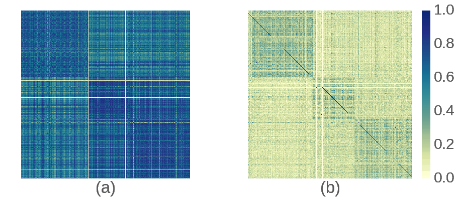
Figure 3: Heat-map showing pair-wise similarities between the learned representations from (a) S2V and (b) N2V-i for the 20 Newsgroups dataset.

4.3 Ranking Results

From Table 9, we observe that over all the summarization tasks, N2V-r, REG-uw, REG-w, DICTREG-uw, and DICTREG-w consistently outshine the baseline S2V model. For DUC 2001, in $10$-length summary, N2V-r wins by $2.21\%$ over S2V, whereas for $100$-length summary, N2V-i wins over S2V by a margin of $5.16\%$. For DUC 2002, REG-w and REG-uw perform better than all other models. For length $10$, REG-w improves over S2V by $2.5\%$, whereas REG-uw gets around $3.26\%$ improvement for length $100$.

In summary, models in Block IV and N2V-r, i.e. models which harness the information content of discourse network during the learning phase have better performance than the other models in the summarization task. Here to note that, N2V-r also retrofits during learning as opposed to IT-w and IT-uw, which retrofit the learned representations as a post-processing step.

		2001			2002
		10	100		10	100
I	S2V	12.65	43.63		14.39	54.51
II	N2V	(+) 1.26	(+) 5.00		($-$) 0.45	($-$) 0.39
	N2V-i	(+) 0.48	(+) 5.16		($-$) 0.87	($-$) 0.45
III	N2V-r	(+) 2.21	(+) 1.88		(+) 0.26	(+) 0.31
	IT-uw	($-$) 0.20	($-$) 1.51		(+) 0.34	($-$) 0.17
	IT-w	(+) 0.04	($-$) 1.02		(+) 0.29	($-$) 1.05
IV	REG-uw	(+) 1.02	(+) 1.31		(+) 2.44	(+) 3.26
	REG-w	(+) 0.74	(+) 1.07		(+) 2.51	(+) 3.10
	DICTREG-uw	(+) 1.79	(+) 1.33		(+) 2.04	(+) 2.71
	DICTREG-w	(+) 1.46	(+) 1.79		(+) 1.63	(+) 2.51

Table 9: Summarization result on DUC 2001-02 datasets for summary lengths of 10 and 100. Here, we present the increment in average recall of a model with reference to the S2V model.

In conclusion, over all the three (3) fundamental information system tasks, models in Block IV consistently improve over the S2V model. The models which use both the content and the information in the discourse network win over the baseline in both the classification and the clustering tasks (Please see the results of Block III and IV in Tables 7 and 8).

5 Related Work

Our work is closely related to two different branches of representational learning research: (i) distributed representation of textual units (e.g., words, paragraphs), and (2) latent representation of nodes in a network.

5.1 Representation for Textual Units

The Word2Vec model [14] to learn distributed representation of words is very popular for text processing tasks. The model also scales well in practice due to its simple architecture.  [12] extended Word2Vec to learn the representation for sentences and documents. The model maps each sentence to an unique id and learns the representation for the sentence using the contexts of words in the sentence – either by predicting the whole context or by predicting a word in the context given the rest. In our work, we extend this model to incorporate inter-sentence relations in the form of a discourse graph. We do this using a graph-smoothing regularizer in the original objective function or by retrofitting the original vectors on the discourse graph.

Recently, [27, 4, 28] propose methods to incorporate semantic knowledge into the word representation models. Our overall idea of using discourse as an extra source of information is reminiscent of these studies with a number of key differences: (i) the semantic network is given in their case, whereas we construct the network using similarities between nodes; (ii) we explore a purely network-based model for learning sentence representations and combine it with the content-based model, whereas they use the network just as an extra source of information in their content-based model. The network-based model gives us the flexibility to adaptively explore the network neighborhood.

Skip-Thought [11] and Fast-Sent [7] are the most recently proposed sentence representation methods. Skip-Thought uses an encoder-decoder approach to reconstruct neighboring sentences of an input sentence, whereas Fast-Sent predicts words from the neighboring sentences for learning representation of the current sentence. Our discourse network is more general and can connect any pair of sentences. Skip-Thought is computationally very expensive [7]. Our approach is fundamentally different from these models and gives a light-weight solution to incorporate discourse.

5.2 Representation for Nodes in Networks

DeepWalk [19], LINE [25] and node2vec [5] are some of the recent advancements on learning representation for nodes in a network, and are closely related to our work. These studies show promising results over linear and non-linear matrix factorization techniques, such as PCA [10], Iso-Map [26], and LLE [21]. They are also related to each other in a sense that they all use discriminative models to learn the representation. These methods differ in how they generate the neighborhood (i.e., context) of a node from the graph. DeepWalk generates contexts using truncated random-walk. Both LINE and node2vec use alias sampling for generating contexts. node2vec uses a controlled random walk to adaptively combine breadth first search and depth first search. In our work, we use node2vec as the network-based model, and we combine it with the content-based model.

6 Conclusion and Future Work

In this paper, we have proposed a set of novel models for learning vector representation of sentences that consider not only content of a sentence but relations among sentences. The relations among sentences are encoded in a discourse graph, which is then used to build discourse informed sentence representation models. We have explored two different ways to incorporate discourse information: (i) by retrofitting the vectors learned from a content-based model on the discourse graph, and (ii) by regularizing the content-based model with a graph smoothing factor.

We evaluated our models on three tasks of classification, clustering, and ranking. Our results show that our models outperform the content-only baseline, and the regularized models perform well in all three tasks whereas the retrofitting models are good for only classification and clustering tasks.

In future, we would like to extend our models to represent groups in social networks and evaluate on prediction tasks involving social groups. The main difference between a network of sentences and a network of social groups is that groups are sets (order is irrelevant), whereas sentences are sequences. However, considering that our content-based model (DBOW) does not take order into account, we should be able to directly apply our models to social groups.

References

- [1] C. F. Baker, C. J. Fillmore, and J. B. Lowe. The berkeley framenet project. In Proceedings of the 36th Annual Meeting of the Association for Computational Linguistics and 17th International Conference on Computational Linguistics-Volume 1, pages 86–90, 1998.
- [2] Y. Bengio, R. Ducharme, P. Vincent, and C. Janvin. A neural probabilistic language model. J. Mach. Learn. Res., 3, Mar. 2003.
- [3] G. Erkan and D. R. Radev. Lexrank: Graph-based lexical centrality as salience in text summarization. J. Artif. Int. Res., 22(1):457–479, Dec. 2004.
- [4] M. Faruqui, J. Dodge, S. K. Jauhar, C. Dyer, E. Hovy, and N. A. Smith. Retrofitting word vectors to semantic lexicons. In Proc. of NAACL, 2015.
- [5] A. Grover and J. Leskovec. node2vec: Scalable feature learning for networks. In Proceedings of the 22nd ACM SIGKDD International Conference on Knowledge Discovery and Data Mining, pages 855–864, 2016.
- [6] F. Hill, K. Cho, and A. Korhonen. Learning distributed representations of sentences from unlabelled data. In Proceedings of the 2016 Conference of the North American Chapter of the Association for Computational Linguistics: Human Language Technologies, pages 1367–1377, San Diego, California, June 2016. Association for Computational Linguistics.
- [7] F. Hill, K. Cho, and A. Korhonen. Learning distributed representations of sentences from unlabelled data. arXiv preprint arXiv:1602.03483, 2016.
- [8] J. R. Hobbs. Coherence and coreference. Cognitive science, 3(1):67–90, 1979.
- [9] T. Joachims. Training linear svms in linear time. In Proceedings of the 12th ACM SIGKDD International Conference on Knowledge Discovery and Data Mining, KDD ’06, pages 217–226, 2006.
- [10] I. Jolliffe. Principal component analysis. Wiley Online Library, 2002.
- [11] R. Kiros, Y. Zhu, R. R. Salakhutdinov, R. Zemel, R. Urtasun, A. Torralba, and S. Fidler. Skip-thought vectors. In Advances in neural information processing systems, pages 3294–3302, 2015.
- [12] Q. V. Le and T. Mikolov. Distributed representations of sentences and documents. In ICML, volume 14, pages 1188–1196, 2014.
- [13] C.-Y. Lin. Rouge: A package for automatic evaluation of summaries. In Text summarization branches out: Proceedings of the ACL-04 workshop, volume 8. Barcelona, Spain, 2004.
- [14] T. Mikolov, K. Chen, G. Corrado, and J. Dean. Efficient estimation of word representations in vector space. arXiv preprint arXiv:1301.3781, 2013.
- [15] T. Mikolov, I. Sutskever, K. Chen, G. Corrado, and J. Dean. Distributed representations of words and phrases and their compositionality. In Proceedings of the 26th International Conference on Neural Information Processing Systems, NIPS’13, pages 3111–3119, 2013.
- [16] G. A. Miller. Wordnet: a lexical database for english. Communications of the ACM, 38(11):39–41, 1995.
- [17] A. Nenkova and K. McKeown. Automatic summarization. Foundations and Trends® in Information Retrieval, 5(2–3):103–233, 2011.
- [18] L. Page, S. Brin, R. Motwani, and T. Winograd. The pagerank citation ranking: bringing order to the web. 1999.
- [19] B. Perozzi, R. Al-Rfou, and S. Skiena. Deepwalk: Online learning of social representations. In Proceedings of the 20th ACM SIGKDD international conference on Knowledge discovery and data mining, pages 701–710. ACM, 2014.
- [20] A. Rosenberg and J. Hirschberg. V-measure: A conditional entropy-based external cluster evaluation measure. In EMNLP-CoNLL, volume 7, pages 410–420, 2007.
- [21] S. T. Roweis and L. K. Saul. Nonlinear dimensionality reduction by locally linear embedding. Science, 290(5500):2323–2326, 2000.
- [22] M. Stede. Discourse processing. Morgan & Claypool Publishers, 2011.
- [23] P. P. Talukdar and K. Crammer. New regularized algorithms for transductive learning. In Proceedings of the European Conference on Machine Learning and Knowledge Discovery in Databases: Part II, ECML PKDD ’09, pages 442–457. Springer-Verlag, 2009.
- [24] J. Tang, M. Qu, and Q. Mei. Pte: Predictive text embedding through large-scale heterogeneous text networks. In Proceedings of the 21th ACM SIGKDD International Conference on Knowledge Discovery and Data Mining, pages 1165–1174. ACM, 2015.
- [25] J. Tang, M. Qu, M. Wang, M. Zhang, J. Yan, and Q. Mei. Line: Large-scale information network embedding. In Proceedings of the 24th International Conference on World Wide Web, pages 1067–1077. ACM, 2015.
- [26] J. B. Tenenbaum, V. De Silva, and J. C. Langford. A global geometric framework for nonlinear dimensionality reduction. science, 290(5500):2319–2323, 2000.
- [27] C. Xu, Y. Bai, J. Bian, B. Gao, G. Wang, X. Liu, and T.-Y. Liu. Rc-net: A general framework for incorporating knowledge into word representations. In Proceedings of the 23rd ACM International Conference on Conference on Information and Knowledge Management, pages 1219–1228. ACM, 2014.
- [28] M. Yu and M. Dredze. Improving lexical embeddings with semantic knowledge. In Proceedings of the 52nd Annual Meeting of the Association for Computational Linguistics (Volume 2: Short Papers), pages 545–550, Baltimore, Maryland, June 2014. Association for Computational Linguistics.