Unifying Type II Supernova Light Curves with Dense Circumstellar Material

Abstract

A longstanding problem in the study of supernovae (SNe) has been the relationship between the Type IIP and Type IIL subclasses. Whether they come from distinct progenitors or they are from similar stars with some property that smoothly transitions from one class to another has been the subject of much debate. Here we show using one-dimensional radiation-hydrodynamic SN models that the multi-band light curves of SNe IIL are well fit by ordinary red supergiants surrounded by dense circumstellar material (CSM). The inferred extent of this material, coupled with a typical wind velocity of $\sim 10-100\,{\rm km\,s^{-1}}$, suggests enhanced activity by these stars during the last $\sim\,$months to $\sim\,$years of their lives, which may be connected with advanced stages of nuclear burning. Furthermore, we find that even for more plateau-like SNe that dense CSM provides a better fit to the first $\sim 20\,$days of their light curves, indicating that the presence of such material may be more widespread than previously appreciated. Here we choose to model the CSM with a wind-like density profile, but it is unclear whether this just generally represents some other mass distribution, such as a recent mass ejection, thick disk, or even inflated envelope material. Better understanding the exact geometry and density distribution of this material will be an important question for future studies.

1. Introduction

Hydrogen-rich supernovae (SNe) have traditionally been divided into Type IIP (plateau) and Type IIL (linear) subclasses based on the shape of their light curves during the first few weeks (Barbon et al., 1979). Beyond just their light curve morphology, these subclasses have other distinguishing features, such as SNe IIL are on average more luminous than SNe IIP by $\sim\,$1.5 mag (Patat et al., 1993, 1994; Anderson et al., 2014; Faran et al., 2014b; Sanders et al., 2015), SNe IIL tend to have redder continua and higher oxygen to hydrogen ratio as compared to ordinary SNe IIP (Faran et al., 2014b), SNe IIL exhibit higher expansion velocities at early times (Faran et al., 2014b), and they have less pronounced P-Cygni H$\alpha$ profiles (Gutiérrez et al., 2014).

These differences have inspired a long debate on whether there is a physical process that smoothly transitions between Type IIP and IIL or whether there is a specific mechanism that creates this distinction more abruptly. Although there have been claims of distinct populations (Arcavi et al., 2012; Faran et al., 2014a, b), support for the more continuous case has increased as larger compilations by Anderson et al. (2014) and Sanders et al. (2015) showed a more continuous range of early light curve slopes. Following this, Valenti et al. (2015) importantly demonstrated that if one simply follows a SN IIL long enough, its light curve will drop at $\sim 100\,{\rm days}$, just like a normal SN IIP (previous SNe IIL studies rarely followed the light curve beyond $\sim 80\,{\rm days}$ from discovery). This implies that Type IIL and Type IIP SNe may share the same basic progenitor, and whatever is creating the Type IIL distinction must be contributing something above the fairly normal underlying red supergiant (RSG).

At the same time, there has been increasing evidence of SNe interacting with dense circumstellar material (CSM) that requires strong mass loss shortly before core collapse (see Smith, 2014, and references therein). This can manifests itself in narrow optical emission lines (Filippenko, 1997; Pastorello et al., 2008; Kiewe et al., 2012; Taddia et al., 2013), X-ray or radio emission (Campana et al., 2006; Corsi et al., 2014), or a rapid rise at ultraviolet wavelengths (Ofek et al., 2010; Gezari et al., 2015; Tanaka et al., 2016; Ganot et al., 2016). In the most extreme cases, there are the super-luminous SNe and SNe IIn events that can require $\sim 10\,M_{\odot}$ or more ejected in the last few years of a massive star’s life (Smith et al., 2007; Smith & McCray, 2007; Woosley et al., 2007; van Marle et al., 2010; Smith et al., 2011; Ofek et al., 2013). Nevertheless, it has also become clear that many other SNe have fleeting signs of CSM interaction where SNe IIn spectral features are seen within a few days of explosion (Gal-Yam et al., 2014; Smith et al., 2015; Khazov et al., 2016). This indicates that smaller, but still dramatic mass loss may be more widespread. In the particular case of PTF11iqb, it transitioned from showing Type IIn-like features to a Type IIL light curve before becoming more IIP-like and finally showing IIn features again (Smith et al., 2015). This suggests an even closer relationship between these SN types and the CSM properties, and that in many cases we might just lack the temporal coverage (especially at early and late times) needed to identify the CSM’s impact.

Motivated by these developments, we undertake a theoretical study on the affect of dense CSM around RSGs on SN light curves, and then conduct detailed comparisons with observed SNe IIP and IIL. We begin in Section 2 by summarizing our numerical methods and presenting a series of simulations to survey the range of ways a dense CSM will alter light curves. In Section 3, we provide a brief overview of SNe 2013ej, 2013by and 2013fs, three SNe for which we then conduct detailed, multi-band fits in Section 4. We discuss the application of our study to the problem of diversity between the SNe IIP and IIL in Section 5, and discuss the implications for the nature of the mass loss inferred from our fits. Finally, we summarize our conclusions in Section 6.

2. Impact of a Dense Wind on Light Curves

We begin by outlining our numerical setup and presenting a series of simulations to explore the impact of a dense wind on SN light curves. This will help provide some guidance on what light curve features can be affected for our later comparison to observations.

2.1. Numerical Setup

Throughout this work we use the non-rotating solar-metallicity RSG models from the stellar evolution code KEPLER (Weaver et al., 1978; Woosley & Heger, 2007, 2015; Sukhbold & Woosley, 2014; Sukhbold et al., 2016). Extending above these models we add a dense CSM, for which we assume a steady-state wind with a density profile

$$\rho(r)=\frac{\dot{M}}{4\pi r^{2}v_{\rm wind}}=\frac{K}{r^{2}},$$ (1)

where $\dot{M}$ is the wind mass loss rate and $v_{\rm wind}$ is the wind velocity. In general, we infer $\dot{M}$ from our models based on the $K$ we are using and the expected $v_{\rm wind}$. This density profile extends out to a radius $R_{\rm ext}$ where we abruptly set the density to zero. This provides us with a useful parameterization for exploring the properties of the CSM (with the main variables being $K$ and $R_{\rm ext}$). It is possible that the CSM may actually be in some other mass distribution, and this wind we consider is just an approximation. We discuss this possibility further in Section 5.

The impact of the dense wind has been investigated in a large number of works (Smith & McCray, 2007; Chugai et al., 2007; Ofek et al., 2010; Chevalier & Irwin, 2011; Moriya et al., 2011). The main difference between our work and these previous studies is that we focus on considerably higher mass losses ($\dot{M}$ in the range of $0.02-15\,M_{\odot}\,{\rm yr}^{-1}$) and small external radii of the wind $900\,R_{\odot}<R_{\rm ext}<2700\,R_{\odot}$. In contrast, for example, Moriya et al. (2011) considers larger radii ($\sim 10^{4}\,R_{\odot}$) and wind mass loss rates in the range of $10^{-4}-10^{-2}\,M_{\odot}\,{\rm yr}^{-1}$. The closest analog to our work is in fact probably the study by Nagy & Vinkó (2016), who consider a two-component model for fitting Type IIP light curves. In particular, both that study and our work here attempt to fit SN 2013ej, and we compare these results below.

These models are then exploded with our open-source numerical code SNEC (Morozova et al., 2015). We assume that the inner $1.4\,M_{\odot}$ of the models form a neutron star and excise this region before the explosion. We use a thermal bomb mechanism for the explosion, adding the energy of the bomb to the internal energy in the inner $0.02\,M_{\odot}$ of the model for a duration of $1\,{\rm s}$. The compositional profiles are smoothed using “boxcar” approach with the same parameters as in Morozova et al. (2015), and the same values for the opacity floor are adopted. The equation of state includes contributions from ions, electrons and radiation, with the degeneracy effects taken into account as in Paczyński (1983). We trace the ionization fractions of hydrogen and helium solving the Saha equations in the non-degenerate approximation as proposed in Zaghloul et al. (2000). The numerical grid consists of 1000 cells and is identical to the one used in Morozova et al. (2015, 2016).

We include the velocity of the wind in our models set to $10\,{\rm km}\,{\rm s}^{-1}$, as in Moriya et al. (2011). Note that the unshocked wind velocities measured from Type IIn SNe are higher than that and vary in the range $10^{2}-10^{3}\,{\rm km}\,{\rm s}^{-1}$ (see Kiewe et al., 2012). The escape velocities of the RSG model that we use vary in the range $75-92\,{\rm km}\,{\rm s}^{-1}$. The exact choice of the wind velocity does not matter in detail though because Moriya et al. (2011) find that the wind velocity has little impact on the final light curve, which we confirm by comparing simulations performed with wind velocities $10$ and $10^{2}\,{\rm km}\,{\rm s}^{-1}$.

2.2. Parameter Survey Results

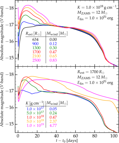
Figure 1.— Top panel: $V$-band light curves of $M_{\rm ZAMS}=12\,M_{\odot}$ RSG model supplemented by a wind with $K=1.0\times 10^{18}\,{\rm g}\,{\rm cm}^{-1}$ and different values of the external radius $R_{\rm ext}$. Bottom panel: $V$-band light curves of the same model supplemented by a wind with a fixed external radius $R_{\rm ext}=1700\,R_{\odot}$ and different values of the density parameter $K$.

For our initial study of the CSM impact, we stitch the dense wind to a RSG model with a zero-age main-sequence (ZAMS) mass of $M_{\rm ZAMS}=12\,M_{\odot}$ for the different values of parameters $R_{\rm ext}$ and $K$. The asymptotic energy of each explosion is $E_{\rm fin}=1.0\times 10^{51}\,{\rm erg}$, and all the models have $0.0207\,M_{\odot}$ of ${}^{56}{\rm Ni}$ mixed up to the mass coordinate $3.5\,M_{\odot}$ (the setup is similar to what we later use for SN 2013ej).

In the top panel of Figure 1, we fix the density parameter $K$ of the wind and vary its external radius. The light curves are plotted relative to the time of shock breakout $t_{0}$ (as are all other light curves in this text). Increasing $R_{\rm ext}$ leads to an increase of the brightness of the early light curve. The brake in the slope of the light curves as the luminosity falls down at around $\sim 15-30$ days coincides with the time when the photosphere in our models passes through the interface between the wind and the underlying RSG model. A more extended wind effectively increases the decline rate of the light curve, making these models promising for understanding SNe IIL (Anderson et al., 2014; Faran et al., 2014a, b; Valenti et al., 2016). The values of $M_{\rm wind}$ quoted in the figure correspond to the total mass of the wind in each case. The more extended winds make the total mass of the model larger and consequently increase the length of the plateau, but this effect is very modest with respect to the impact on the early light curve.

In the bottom panel of Figure 1, we fix the external radius of the wind and vary the parameter $K$. This corresponds to everything from very low wind masses to a few especially extreme cases where the wind is so extreme that it completely dominates over the RSG. From this panel one can see that there is a degeneracy in the way in which the radius and the density of the wind impact the light curve. The more extended and less dense winds produce light curves that are similar to the more compact and dense winds (to see it, one can compare the green, red and blue light curves in both panels and notice the parameters to which these light curves correspond). This degeneracy will be seen in Section 4.2, when we attempt to fit the observational data with the light curves from our grid.

3. Overview of the Supernovae

Given our result that varying $R_{\rm ext}$ seems to naturally transition from slow to fast early declining SNe (basically, from SNe IIP to IIL), we would next like to fit specific examples to see what properties are inferred about the stars and their CSM environment. Due to the many parameters involved in such fitting (e.g., $M_{\rm ZAMS}$, $E_{\rm fin}$, $R_{\rm ext}$, $K$), this is a time consuming process. So for the present work, we focus on three particularly well-studied events. These have been chosen for their good multi-band light curve coverage. They also span a range of early decline rates, with SN 2013by being the most IIL-like, SN 2013ej having an early decline somewhat between a IIL and IIP, and SN 2013fs having a mostly flat light curve like a IIP but also showing a particularly short plateau (see Figure 4) that is usually observed in IIL-like objects. This way we can see what variety of corresponding CSM properties are inferred. Below we summarize their main properties before fitting them in detail in Section 4.

3.1. SN 2013ej

SN 2013ej has a moderate early decline, thus we consider it transitional between a Type IIL and IIP. It was discovered on 2013 July 25.45 (UT), less than 1 day after the last non-detection, by the Lick Observatory Supernova Search (see Kim et al., 2013; Shappee et al., 2013; Valenti et al., 2013). Details of its early photometric and spectroscopic observations may be found in Valenti et al. (2014), while for the analysis of the pre-explosion image obtained with the Hubble Space Telescope (HST) see Fraser et al. (2014). Originally classified as Type IIP, this SN was reclassified later as Type IIL, based on a fast ($1.74\,{\rm mag}/100\,{\rm days}$ in $V$-band) decline rate of the luminosity as well as relatively slow decline of the H$\alpha$ and H$\beta$ velocity profiles, which are characteristic for this subclass (see Bose et al., 2015; Faran et al., 2014a, b).

A range of features observed in SN 2013ej points to a possible interaction of the ejecta with the CSM. Among them, an unusually strong absorption feature found in the blue wing of the H$\alpha$ P-Cygni trough (see Leonard et al., 2013; Chugai et al., 2007). The presence of high-velocity components in H$\alpha$ and H$\beta$ profiles, demonstrated in the work of Bose et al. (2015), also suggests an interaction. At the same time, the presence of CSM surrounding SN 2013ej was supported by the X-ray measurements taken by Swift and Chandra instruments (Margutti et al., 2013a). Chakraborti et al. (2016) analyzed these data and found them consistent with the steady progenitor wind scenario. According to their model, the progenitor star lost mass at the rate $3\times 10^{-6}\,M_{\odot}\,\mathrm{yr}^{-1}$ assuming $v_{\rm wind}\sim 10\,\mathrm{km}\,\mathrm{s}^{-1}$ for the last $400$ years.

Spectropolarimetric analysis of SN 2013ej performed by Leonard et al. (2013) revealed significant polarization of $1.0-1.3\%$ at the early epoch ($\sim$day 7 since explosion). Broad-band polarimetric analysis of the late ($>100$ days) phase of this SN performed by Kumar et al. (2016) also shows unusually strong intrinsic polarization up to $2.14\%$. This could be a signal of possible asymmetry in the ejecta.

SN 2013ej was previously modeled semi-analytically in the work of Bose et al. (2015), where its ejecta mass, radius and explosion energy were estimated to be $12\,M_{\odot}$, $450\,R_{\odot}$ and $2.3\times 10^{51}\,{\rm erg}$, respectively. Hydrodynamical simulations of Huang et al. (2015) suggest an ejecta mass of $\sim 10.6\,M_{\odot}$, a radius of the progenitor of $\sim 600\,R_{\odot}$, and an explosion energy $\sim 0.7\times 10^{51}\,{\rm erg}$ for this SN. Yuan et al. (2016) estimate the mass of the progenitor to be $12-15\,M_{\odot}$ at ZAMS, based on the modeling of the nebular emission lines. Dhungana et al. (2016) use the approach of Litvinova & Nadezhin (1983) to derive the final pre-explosion progenitor mass of $15.2\pm 4.2\,M_{\odot}$, progenitor radius of $250\pm 70\,R_{\odot}$ and explosion energy $0.9\pm 0.3\times 10^{51}\,{\rm erg}$.

3.2. SN 2013by

SN 2013by had a particularly steep luminosity decline ($1.46\pm 0.06\,{\rm mag}$ in $V$-band) in the first 50 days, and we consider this representative of a IIL-like event. It was discovered on 2013 April 23.54 (UT) by the Backyard Observatory Supernova Search (Parker et al., 2013). It was classified as a young SN IIL/IIn based on early optical and near infrared observations, which was further confirmed by a detailed analysis of Valenti et al. (2015). Possible interaction of the ejecta with the CSM is supported by the X-ray observations obtained with Swift (see Margutti et al., 2013b). It also showed a very pronounced drop before transitioning to the ${}^{56}{\rm Ni}$ tail, which is typical for SNe IIP. In fact, it was shown in Valenti et al. (2015) that this drop is demonstrated to a greater or lesser extent by all of the SNe IIL that have been followed for long enough (more than $\sim 80$ days since the discovery).

3.3. SN 2013fs

SN 2013fs has a mostly flat light curve and is the most IIP-like of all the events we consider. It was discovered on 2013 Oct. 07.46 (UT) by Koichi Itagaki (Teppo-cho, Yamagata, Japan) (Nakano et al., 2013). The first spectrum taken on Oct 08 with the Wide Field Spectrograph was reported in Childress et al. (2013b) and demonstrated extremely blue, nearly featureless continuum, exhibiting slightly broadened emission in H$\alpha$ and H$\beta$. This led to the preliminary classification of the object as a SN IIn. However, the next spectrum taken on Oct 24 had no evidence of broadened emission and strongly resembled a normal SN IIP spectrum (Childress et al., 2013a). Analysis of the observational data of SN 2013fs has not yet been presented in an individual paper, and the present work is the first attempt to model the data numerically.

4. Fitting the Observed Light Curves with Numerical Models

Next we construct a grid of models and fit the multi-band light curves of the three SNe II that are described above. We first discuss the methods to our analysis in Section 4.1 and then present results of our fitting in Section 4.2. A more detailed discussion of the implications of these fits is provided later in Section 5.

4.1. Analysis

For our grid of models, we consider a 4-dimensional parameter space in $M_{\rm ZAMS}$, $E_{\rm fin}$, $K$, and $R_{\rm ext}$. The external radius of the wind $R_{\rm ext}$ in our models varies between $900\,R_{\odot}$ and $2700\,R_{\odot}$ in steps of $200\,R_{\odot}$, and $K$ takes the values $\{1.0,2.5,5.0,7.5\}\times 10^{17}\,{\rm g}\,{\rm cm}^{-1}$, $\{1.0,2.5,5.0,7.5\}\times 10^{18}\,{\rm g}\,{\rm cm}^{-1}$ and $\{1.0,2.5,5.0,7.5\}\times 10^{19}\,{\rm g}\,{\rm cm}^{-1}$. We use non-rotating solar-metallicity RSG models from the stellar evolution code KEPLER (Weaver et al., 1978; Woosley & Heger, 2007, 2015; Sukhbold & Woosley, 2014; Sukhbold et al., 2016) with ZAMS masses in the range between $9\,M_{\odot}$ and $16.5\,M_{\odot}$. These are spaced in steps of $0.25\,M_{\odot}$ in the interval $9\,M_{\odot}\leq M_{\rm ZAMS}\leq 13\,M_{\odot}$, and in steps of $0.5\,M_{\odot}$ in the interval $13\,M_{\odot}<M_{\rm ZAMS}\leq 16.5\,M_{\odot}$. The asymptotic explosion energy $E_{\rm fin}$ (not to be confused with the inputted thermal bomb energy) varies in individual ranges for each SN. Namely, in the case of SN 2013ej, the energy varies in the range $(0.4-2.6)\times 10^{51}\,{\rm erg}$ for the grid without wind, and in the range $(0.4-1.4)\times 10^{51}\,{\rm erg}$ for the grid with the wind, both in steps of $0.2\times 10^{51}\,{\rm erg}$. For SN 2013by the corresponding ranges are $(0.8-3.0)\times 10^{51}\,{\rm erg}$ (without wind) and $(1.0-2.0)\times 10^{51}\,{\rm erg}$ (with wind), and for SN 2013fs the ranges are $(0.4-2.6)\times 10^{51}\,{\rm erg}$ and $(0.6-1.6)\times 10^{51}\,{\rm erg}$. These ranges were chosen so that the fitting parameters are located well inside the grid to maximize computing resources.

In addition to the grid, for each SN we use a fixed mass of radioactive nickel $M_{\rm Ni}$, which was taken from the supporting information in Valenti et al. (2016). This gives $M_{\rm Ni}=0.0207\pm 0.0019$ for SN 2013ej, $0.032\pm 0.0043$ for SN 2013by, and $0.0545\pm 0.0003$ for SN 2013fs. In all models we mix the ${}^{56}{\rm Ni}$ up to the mass coordinate $3.5\,M_{\odot}$ and do not vary this parameter.

Before comparing the numerical models with the data, we corrected the multi-band light curves for reddening using the Cardelli law (see Cardelli et al., 1989). The following values for the absorption in $B$-band were used: $A_{B}=0.25\,{\rm mag}$ for SN 2013ej, $A_{B}=0.798\,{\rm mag}$ for SN 2013by and $A_{B}=0.145\,{\rm mag}$ for SN 2013fs. In all three SNe, the reddening is due to the Milky Way, while the contribution from the host galaxy is negligible. The distance moduli are $\mu=29.79\pm 0.02$ for SN 2013ej, $\mu=30.84\pm 0.15$ for SN 2013by and $\mu=33.50\pm 0.15$ for SN 2013fs (Valenti et al., 2016).

For each of the three SNe we assess the best fitting model within the generated grids of light curves by calculating $\chi^{2}$ as

$$\chi^{2}=\sum_{\lambda\in[g,...,z]}\,\,\,\sum_{t^{*}<t_{PT}}\frac{(M_{\lambda}^{*}(t^{*})-M_{\lambda}(t^{*}))^{2}}{M_{\lambda}(t^{*})}\ ,$$ (2)

where $M_{\lambda}^{*}(t^{*})$ is the observed magnitude in a given band $\lambda$ at the moment of observation $t^{*}$, $M_{\lambda}(t^{*})$ is the numerically obtained magnitude in the same band at the same moment of time, and $t_{PT}$ is the length of plateau as defined in the work of Valenti et al. (2016). This is taken to be $99\,{\rm days}$ for SN 2013ej, $85\,{\rm days}$ for SN 2013by and $83\,{\rm days}$ for SN 2013fs. We restrict our fits to the plateau phase, because during the radioactive tail we do not expect the spectrum to be well described by a black body, as assumed in SNEC. The best fitting model corresponds to the minimum value of $\chi^{2}$. We include in the $\chi^{2}$ all bands redder than $g$-band and do not include $B$-, $u$- and $U$-bands, since the light curves in these bands are affected by iron group line blanketing (Kasen & Woosley, 2009), which is not taken into account in SNEC.

When calculating $\chi^{2}$, we do not take into account the observational errors, because their values may differ by an order of magnitude for different epochs. Taking into account the error bars leads to a visually worse fit, because the best fitting model tends to fit a few particular points with the least error instead of fitting the entire light curve.

Figure 2.— Best fits of the SN 2013ej data without (dashed lines) and with (solid lines) CSM.

4.2. Fitting Results

Figures 2 to 4 show the data in different bands for the three considered SNe, together with our best fitting models with (solid lines) and without (dashed lines) CSM. The white (unshaded) regions in the plots contain the data which was used in order to calculate the fits, while the data from the gray (shaded) regions was not used in our analysis. Comparing the dashed lines with the data in Figures 2 to 4 demonstrate that none of the light curves obtained from the RSG models without wind can reproduce the data well. Without a wind, the light curves are not sufficiently peaked at early times. The fitting routine compensates for this by “splitting the difference” and overshooting the data during the plateau phase. In contrast, the models that include a wind provide a much better fit across all the data.

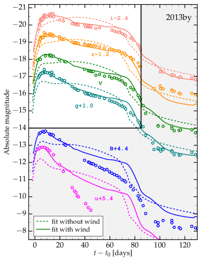
Figure 3.— Best fits of the SN 2013by data without (dashed lines) and with (solid lines) CSM.

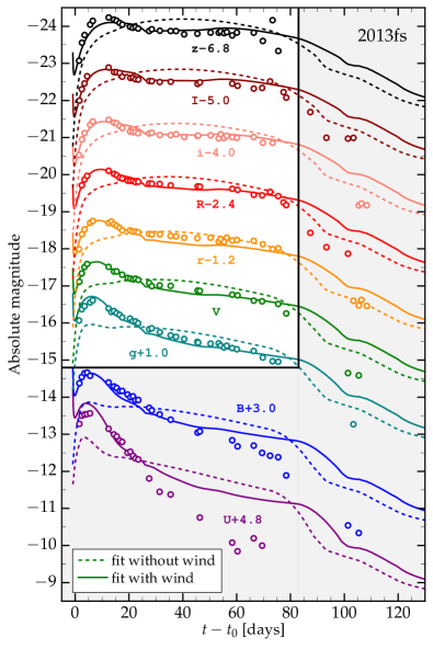
Figure 4.— Best fits of the SN 2013fs data without (dashed lines) and with (solid lines) CSM.

It is interesting to note that our models with the wind even reproduce reasonably well the early parts of the $u$-, $U$- and $B$-data, which we did not explicitly used to find the fit. Large discrepancies between our light curves and the data in these bands at later times can be explained by the iron group line blanketing, which is not taken into account in SNEC. In the work of Kasen & Woosley (2009), it was shown that this effect starts playing an important role for the blue bands after few tens of days. Similarly, our results suggest that for the first $\sim 10-20$ days the effect of the iron group line blanketing is not so strong, and the spectrum can be well described by a black body. The transition between the plateau and ⁵⁶Ni tail is sensitive to the low temperature opacities, which are not well known, as well as to the degree of mixing of ⁵⁶Ni, which we did not vary in this study because it would just be too many parameters to fit. So we do not view places where we are not able to reproduce the data during this phase as a failure of the model.

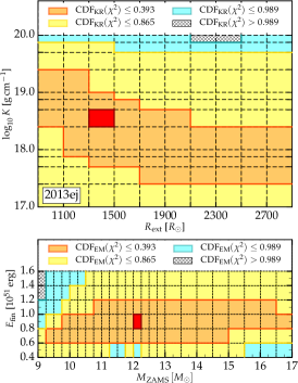
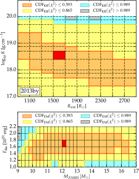
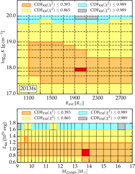
Figure 5.— Top panels: 2D slices ($E_{\rm fin}=E_{\rm fin,fit}$, $M_{\rm ZAMS}=M_{\rm ZAMS,fit}$) of the 4D parameter space for SN 2013ej, SN 2013by and SN 2013fs. Bottom panels: 2D slices ($R_{\rm ext}=R_{\rm ext,fit}$, $K=K_{\rm fit}$) of the 4D parameter space for SN 2013ej, SN 2013by and SN 2013fs. Confidence regions correspond to the $1$, $2$ and $3$ standard deviations of the mean of a two-dimensional symmetric Gaussian (see text for additional details).

Figure 5 shows the position of the fitting parameters for the SNe 2013ej, 2013by and 2013fs. The top panels of the figure show the $K-R_{\rm ext}$ slice of the 4D parameter space, where the values of $M_{\rm ZAMS}$ and $E_{\rm fin}$ are set equal to the fitting values. The bottom panels of the figure shows the $M_{\rm ZAMS}-E_{\rm fin}$ slice of the 4D parameter space, where the values of $R_{\rm ext}$ and $K$ are set equal to the fitting values. Red blocks in all the plots denote the best fitting parameters, which we summarize in Table 1. To evaluate the robustness of the fits, we show the $39.3\%$, $86.5\%$ and $98.9\%$ confidence regions, which correspond to the one, two and three standard deviations of the mean of a two-dimensional Gaussian.

One can see from Figure 5 that there are strong degeneracies in some of the parameters. The confidence interval in the $K-R_{\rm ext}$ plane has a characteristic “banana” shape, in the sense that the models with extended low density wind produce similar fits to the models with less extended high density wind. Also, $M_{\rm ZAMS}$ is difficult to completely constrain because a large part of the light curve we are fitting is hidden by the CSM. This is not surprising since Kasen & Woosley (2009) show that the length of the plateau is only weakly dependent on the ejecta mass. Nevertheless, it is robust that light curves with a dense wind do a dramatically better job at fitting the data than those without.

It is also interesting to compare our best fit parameters for SN 2013ej to the results of Nagy & Vinkó (2016), who use a semi-analytic, two-component model to fit the same SN. They find a mass and radius for what they call the “envelope” material of $0.6\,M_{\odot}$ and $980\,R_{\odot}$, respectively, while for our wind we find $0.7\,M_{\odot}$ and $1300\,R_{\odot}$. Given the difference in techniques (they focus on fitting bolometric light curves while we are fitting various photometric bands with numerical models), the similarity of these inferred parameters is encouraging. The fact that Nagy & Vinkó (2016) extend this sort of fitting to a variety of other well-studied Type IIP-like SNe argues that a similar amount of CSM as we infer for SN 2013ej may be present in a wide range of otherwise seemingly “normal” events.

Table 1Best Fit Parameters

Name	$M_{\rm ZAMS,fit}\,[M_{\odot}]$	$E_{\rm fin,fit}\,[10^{51}\,{\rm erg}]$	$K_{\rm fit}\,[{\rm g}\,{\rm cm}^{-1}]$	$R_{\rm ext,fit}\,[R_{\odot}]$	$\dot{M}\,[M_{\odot}\,{\rm yr}^{-1}]$	$t_{\rm wind}$
SN 2013ej	12.0	0.8	$2.5\times 10^{18}$	1300	0.5 (5.0)	$1.5\,{\rm yr}$ ($1.8\,{\rm months}$)
SN 2013by	12.0	1.6	$2.5\times 10^{18}$	1500	0.5 (5.0)	$1.9\,{\rm yr}$ ($2.3\,{\rm months}$)
SN 2013fs	13.5	0.8	$7.5\times 10^{17}$	1900	0.15 (1.5)	$2.5\,{\rm yr}$ ($3.0\,{\rm months}$)

5. Discussion

Next we discuss some of the general trends that are seen in these fits, the physics that produces these features, and the implications for the exploding progenitors given the CSM properties we infer. This includes both what the progenitors look like and what physical processes may have caused them to be this way.

5.1. Light Curve Properties

Figure 6 shows the density profiles of the best fitting models for SNe 2013ej, 2013by and 2013fs as a function of mass (top panel) and radius (bottom panel). They are quite similar to each other, with the models for SNe 2013ej and 2013by differing only by the external radius of the wind. In the wind picture, this would just correspond to a similar $\dot{M}$ but a different amount of time between the start of the wind and explosion, in this case a difference of $\sim 100\,$days depending on the wind velocity. To understand how this impacts the light curve, one can draw an analogy between these models and the extended envelopes considered in the context of double-peaked SNe IIb (Nakar & Piro, 2014; Piro, 2015). Here, instead of the low density extended material attached to a compact core, we have the wind surrounding higher density RSG models. For this kind of progenitors, the initial brightness and fast rise of the light curve are explained by the cooling emission from the low density material (wind), which does not experience strong adiabatic losses due to its initially large volume. The maximum in the optical bands for these progenitors correspond to the moment, when the luminosity shell (the depth from which photons diffuse to reach the photosphere at a given time after shock breakout) reaches the interface between the low density and the high density material (see discussion in Nakar & Piro, 2014).

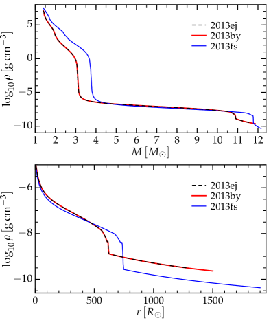
Figure 6.— Density profiles of the best fitting models as a function of mass coordinate (top panel) and radial coordinate (bottom panel) as summarized in Table 1. The progenitor models for SN 2013ej and SN 2013by differ only by $R_{\rm ext}$.

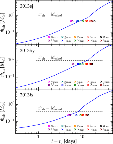
Figure 7.— $\hat{m}_{\rm sh}$, the difference between the total mass of the model and the mass coordinate of the luminosity shell, as a function of time since shock breakout ($t_{0}$) for the best fitting models of SN 2013ej, SN 2013by and SN 2013fs. Crosses indicate the times of maxima in the corresponding bands. Maxima in the optical bands approximately coincide with the moment when the luminosity shell crosses the interface between the RSG model and the wind, $\hat{m}_{\rm sh}=M_{\rm wind}$.

To illustrate this, Figure 7 shows the time dependence of $\hat{m}_{\rm sh}$, which is defined as the difference between the total mass of the progenitor and the mass coordinate of the luminosity shell, for the three fitting models. The position of the luminosity shell is found from the condition $\hat{t}_{\rm diff}=t-t_{0}$, where $t_{\rm diff}=t_{\rm diff}(r,t)$ is the diffusion time at each moment of time and at each depth, and the hat indicates the value of this quantity taken specifically at the luminosity shell (Nakar & Sari, 2010). The diffusion time is computed using

$$\hat{t}_{\rm diff}=\int_{\hat{r}}^{R_{\rm ext}}\frac{3\tau dr}{c},$$ (3)

where

$$\tau(r)=\int_{r}^{R_{\rm ext}}\kappa\rho dr,$$ (4)

and $\hat{r}$ is the radius of the diffusion depth (see Morozova et al., 2016, for more details). From Figure 7 it is clear that the slope of $\hat{m}_{\rm sh}$ as a function of time changes abruptly when the luminosity shell passes the interface between the wind and the underlying RSG model, $\hat{m}_{\rm sh}=M_{\rm wind}$. At the same time, the light curves in the optical bands pass through their maxima shown by the crosses in the plots

5.2. The Origin of the SN IIL Classification

The results of our fitting argue that the origin of SNe IIL is the addition of dense CSM, relatively closely position to the star. This is in contrast to a number of previous studies that explored reducing the mass of the progenitor in order to get SN IIL-like light curves (Blinnikov & Bartunov, 1993; Morozova et al., 2015; Moriya et al., 2016), but similar to the suggestion in Smith et al. (2015) from the observation of PTF11iqb. Even beyond our modeling though, all three of the considered SNe demonstrated some signs of CSM interaction in the observations, as we emphasize in Section 3, strengthening our conclusions. In this picture, continuous transition between the SNe IIP and IIL (Anderson et al., 2014; Sanders et al., 2015) is naturally explained by the continuity in the wind properties of the progenitors. Also, this approach naturally explains observed positive correlation between the maximum brightness and the decline rate of SNe (Anderson et al., 2014), because adding the wind to the progenitor profile increases both of these two observables. We note that the longstanding tradition of presenting groups of SNe IIP and IIL aligned at maximum brightness may have been somewhat misleading because it suggested that the SNe IIL had something missing when in fact they have something added in comparison to a typical RSG.

The question of whether all SNe IIL demonstrate (at least moderate) interaction with CSM has been already raised in Valenti et al. (2015) and discussed in Bose et al. (2015), but our work highlights even more how important this is to investigate. In some cases, these interactions appear through narrow lines seen at early times (Gal-Yam et al., 2014; Smith et al., 2015; Khazov et al., 2016). For the spherically symmetric calculations we perform here, the wind is always optically thick and may appear at odds with these observations. This can be reconciled though if there is additional low density material above the wind that we are calculating. Another possibility is if the CSM is non-spherical, so that the component we are calculating represents regions where the shock can pass into the CSM. In such a case, narrow lines may be formed by tenuous material above and below the CSM, and would therefore disappear once the ejecta overtakes the CSM within a matter of $\lesssim 2\,$days (given the radii we are inferring for it). Therefore to see spectral signatures of the CSM requires getting spectra as soon after explosion as possible. Furthermore, depending on the geometry of the CSM, not all of it may be disrupted by the explosion, and some may still be present once the ejecta has passed. This has in fact been seen for PTF11iqb, for which it was argued that the CSM may be in the form of a disk (Smith et al., 2015). Thus it may also be helpful to perform late observations on SNe with a fast early decline to identify how ubiquitous such features are.

5.3. Implications for the Stellar Progenitors of SNe IIL

Up to now, pre-explosion imaging has not revealed any clear distinction between the progenitors of Type IIP and Type IIL SNe neither in radius (Gall et al., 2015) nor in mass (Valenti et al., 2016). Since our winds are optically thick, the radius we are finding $R_{\rm ext}$ would act as a “pseudo-photosphere,” making the progenitors much redder and potentially dimmer if dust formation occurs. This may appear to be at odds with the pre-explosion imaging. Unfortunately, most pre-explosion imaging is not close enough to time of explosion to probe this CSM given the timescales we are inferring (see Table 1). For example, SN 2009kr was a IIL inferred to have a reasonably normal progenitor radius of $\sim 400-800\,R_{\odot}$, which is consistent with the radii of standard RSGs (Levesque et al., 2005, 2006). Unfortunately, this was done with HST imaging that occurred between $\sim 10$ and $\sim 2\,$yrs before explosion (Fraser et al., 2010; Elias-Rosa et al., 2011). In another case, SN 2013ej (which is one of the events we studied here) was inferred to have a radius $\sim 400-800\,R_{\odot}$ (Valenti et al., 2014; Fraser et al., 2014), but again this is for HST imaging between $\sim 10$ to $8\,$yrs before the SN in comparison to the $\lesssim 2\,$yrs we infer for this event.

Our results highlight that pre-explosion imaging will be needed within $\sim\,$yr of explosion to provide meaningful constraints on the CSM environment that may be turning these events into SNe IIL. Furthermore, given the large radii we infer, these progenitors should be extremely red if not also extinguished by dust. This would make them look anomalously dim at optical wavelengths so that they are mistaken for lower mass stars unless infrared coverage is available.

5.4. Source of the Circumstellar Material

The mass loss rates quoted in Table 1 are much higher than the ones observed for steady winds in RSGs (Nieuwenhuijzen & de Jager, 1990). Even for the extremely dense wind of the most luminous known RSG (VY CMa, Smith et al., 2009) the estimated mass loss rate is $1-2\times 10^{-3}\,M_{\odot}\,{\rm yr}^{-1}$. At the same time, analysis of the emission lines of Type IIn SNe suggests rather strong winds before the explosion (see Kiewe et al., 2012; Smith, 2014, but note higher wind velocities than ours). This suggests that the CSM we are modeling as a wind may not be a wind at all but represent a more explosive outburst rather than something steady.

There is increasing evidence that violent outbursts are important in the final stages of the lives of massive stars. This evidence can come in the form of direct detections of pre-SN outbursts (e.g., Foley et al., 2007; Pastorello et al., 2007; Smith et al., 2010; Foley et al., 2011; Mauerhan et al., 2013; Pastorello et al., 2013) or inferred from the dense CSM needed to explain SN light curves (e.g., Smith & McCray, 2007; Smith et al., 2007; Ofek et al., 2007; Smith et al., 2008; Fransson et al., 2014). Although how common such eruptions are is still being investigated (see Ofek et al., 2014; Bilinski et al., 2015), our work may indicate that SNe IIL are just lower mass versions of these. It is interesting to note that the time of the wind $t_{\rm wind}$ given in Table 1 is comparable to the duration of the carbon shell burning for an $M_{\rm ZAMS}=12\,M_{\odot}$ star (see Fuller et al., 2015). Increasing velocity of the wind by a factor of $10$ would boost the mass loss rates to even larger values, but in this case $t_{\rm wind}$ would coincide with the duration of the oxygen shell burning ($\sim$few months). A better measurement of the extent of the CSM along with its velocity may help to better connect its properties with various stages of stellar burning. This will assist in identifying its physical origin (see discussions in Smith & Arnett, 2014; Woosley & Heger, 2015; Quataert et al., 2016, and references therein).

In these explosive scenarios, the CSM is likely not to have the density profile of a steady wind as we have assumed. In such cases, the radius and mass we infer is probably just an estimate for the true CSM properties. There may also be other possibilities. For example, the CSM we are inferring could be an inflated outer radius of the star, perhaps driven by additional energy input during the end of the star’s life (e.g., like from waves, Quataert & Shiode, 2012; Shiode & Quataert, 2014). Another possibility is that the material could be in the form of a disk as discussed above for PTF11iqb (Smith et al., 2015). In any case, better pre-explosion imaging, early observations during the first $\sim 1\,$day after explosion, and the theoretical modeling of various CSM distributions should help piece together the true properties of the CSM surrounding SNe IIL.

6. Conclusion

We have numerically investigated the light curves of RSGs with CSM. These vary from most previous theoretical studies in that the winds we consider are generally more dense and are rather compact, only extending a few stellar radii above the RSG. We found that the corresponding light curves show many of the hallmarks of SNe IIL and then fit the observations of three particular well-studied SNe II with RSG plus CSM models. The key inferred properties of the CSM are mass loss rates of $\sim 0.1-0.5\,M_{\odot}\,{\rm yr}^{-1}$ and an extent of $\sim 1300-1900\,R_{\odot}$, which implies that the CSM was generated $\lesssim 1-2\,$yrs prior to explosion. This may indicate that this material may be driven by certain advanced stages of stellar burning, but since these estimates depend on the uncertain velocity of the CSM, it is possible that it may be occurring on shorter timescales.

Our results highlight that pre-explosion imaging $\lesssim 1\,$yr prior to explosion and spectra taken $\lesssim 2\,$days following explosion will be key for investigating the properties of this CSM. There should be trends between the early time light curve slope and the inferred CSM properties, and these need to be explored to build a more complete picture on the nature of the CSM. In other cases, one might expect signatures of the CSM to pop up at later times like PTF11iqb (Smith et al., 2015), depending on its radial and latitudinal distribution. Surveys with rapid cadences, such as the Zwicky Transient Facility (Law et al., 2009) and the All-sky Automated Survey for Supernovae (Shappee et al., 2014) make this an ideal time to identify SNe early, so that these critical spectra can be taken. The Large Synoptic Survey Telescope (LSST Science Collaboration et al., 2009) could be also useful in this respect depending on its final cadence. Nevertheless, LSST could also be helpful for having an archive of good time coverage for these progenitors before they explode. This way after the SNe are discovered, their history can be investigated to see whether they showed any pre-explosion outbursts or enhanced winds as we infer here.

References

- Anderson et al. (2014) Anderson, J. P., González-Gaitán, S., Hamuy, M., et al. 2014, ApJ, 786, 67
- Andrae (2010) Andrae, R. 2010, ArXiv e-prints
- Arcavi et al. (2012) Arcavi, I., Gal-Yam, A., Cenko, S. B., et al. 2012, ApJ, 756, L30
- Barbon et al. (1979) Barbon, R., Ciatti, F., & Rosino, L. 1979, A&A, 72, 287
- Bilinski et al. (2015) Bilinski, C., Smith, N., Li, W., et al. 2015, MNRAS, 450, 246
- Blinnikov & Bartunov (1993) Blinnikov, S. I., & Bartunov, O. S. 1993, A&A, 273, 106
- Bose et al. (2015) Bose, S., Sutaria, F., Kumar, B., et al. 2015, ApJ, 806, 160
- Campana et al. (2006) Campana, S., Mangano, V., Blustin, A. J., et al. 2006, Nature, 442, 1008
- Cardelli et al. (1989) Cardelli, J. A., Clayton, G. C., & Mathis, J. S. 1989, ApJ, 345, 245
- Chakraborti et al. (2016) Chakraborti, S., Ray, A., Smith, R., et al. 2016, ApJ, 817, 22
- Chevalier & Irwin (2011) Chevalier, R. A., & Irwin, C. M. 2011, ApJ, 729, L6
- Childress et al. (2013a) Childress, M., Scalzo, R., Yuan, F., Schmidt, B., & Tucker, B. 2013a, The Astronomer’s Telegram, 5527
- Childress et al. (2013b) —. 2013b, The Astronomer’s Telegram, 5455
- Chugai et al. (2007) Chugai, N. N., Chevalier, R. A., & Utrobin, V. P. 2007, ApJ, 662, 1136
- Corsi et al. (2014) Corsi, A., Ofek, E. O., Gal-Yam, A., et al. 2014, ApJ, 782, 42
- Dhungana et al. (2016) Dhungana, G., Kehoe, R., Vinko, J., et al. 2016, ApJ, 822, 6
- Elias-Rosa et al. (2011) Elias-Rosa, N., Van Dyk, S. D., Li, W., et al. 2011, ApJ, 742, 6
- Faran et al. (2014a) Faran, T., Poznanski, D., Filippenko, A. V., et al. 2014a, MNRAS, 445, 554
- Faran et al. (2014b) —. 2014b, MNRAS, 442, 844
- Filippenko (1997) Filippenko, A. V. 1997, ARA&A, 35, 309
- Foley et al. (2011) Foley, R. J., Berger, E., Fox, O., et al. 2011, ApJ, 732, 32
- Foley et al. (2007) Foley, R. J., Smith, N., Ganeshalingam, M., et al. 2007, ApJ, 657, L105
- Fransson et al. (2014) Fransson, C., Ergon, M., Challis, P. J., et al. 2014, ApJ, 797, 118
- Fraser et al. (2010) Fraser, M., Takáts, K., Pastorello, A., et al. 2010, ApJ, 714, L280
- Fraser et al. (2014) Fraser, M., Maund, J. R., Smartt, S. J., et al. 2014, MNRAS, 439, L56
- Fuller et al. (2015) Fuller, J., Cantiello, M., Lecoanet, D., & Quataert, E. 2015, ApJ, 810, 101
- Gal-Yam et al. (2014) Gal-Yam, A., Arcavi, I., Ofek, E. O., et al. 2014, Nature, 509, 471
- Gall et al. (2015) Gall, E. E. E., Polshaw, J., Kotak, R., et al. 2015, A&A, 582, A3
- Ganot et al. (2016) Ganot, N., Gal-Yam, A., Ofek, E. O., et al. 2016, ApJ, 820, 57
- Gezari et al. (2015) Gezari, S., Jones, D. O., Sanders, N. E., et al. 2015, ApJ, 804, 28
- Gutiérrez et al. (2014) Gutiérrez, C. P., Anderson, J. P., Hamuy, M., et al. 2014, ApJ, 786, L15
- Huang et al. (2015) Huang, F., Wang, X., Zhang, J., et al. 2015, ApJ, 807, 59
- Kasen & Woosley (2009) Kasen, D., & Woosley, S. E. 2009, ApJ, 703, 2205
- Khazov et al. (2016) Khazov, D., Yaron, O., Gal-Yam, A., et al. 2016, ApJ, 818, 3
- Kiewe et al. (2012) Kiewe, M., Gal-Yam, A., Arcavi, I., et al. 2012, ApJ, 744, 10
- Kim et al. (2013) Kim, M., Zheng, W., Li, W., et al. 2013, Central Bureau Electronic Telegrams, 3606
- Kumar et al. (2016) Kumar, B., Pandey, S. B., Eswaraiah, C., & Kawabata, K. S. 2016, MNRAS, 456, 3157
- Law et al. (2009) Law, N. M., Kulkarni, S. R., Dekany, R. G., et al. 2009, PASP, 121, 1395
- Leonard et al. (2013) Leonard, P. b. D. C., Pignata, G., Dessart, L., et al. 2013, The Astronomer’s Telegram, 5275
- Levesque et al. (2005) Levesque, E. M., Massey, P., Olsen, K. A. G., et al. 2005, ApJ, 628, 973
- Levesque et al. (2006) —. 2006, ApJ, 645, 1102
- Litvinova & Nadezhin (1983) Litvinova, I. I., & Nadezhin, D. K. 1983, Ap&SS, 89, 89
- LSST Science Collaboration et al. (2009) LSST Science Collaboration, Abell, P. A., Allison, J., et al. 2009, ArXiv e-prints
- Margutti et al. (2013a) Margutti, R., Chakraborti, S., Brown, P. J., & Sokolovsky, K. 2013a, The Astronomer’s Telegram, 5243
- Margutti et al. (2013b) Margutti, R., Soderberg, A., & Milisavljevic, D. 2013b, The Astronomer’s Telegram, 5106
- Mauerhan et al. (2013) Mauerhan, J. C., Smith, N., Filippenko, A. V., et al. 2013, MNRAS, 430, 1801
- Moriya et al. (2011) Moriya, T., Tominaga, N., Blinnikov, S. I., Baklanov, P. V., & Sorokina, E. I. 2011, MNRAS, 415, 199
- Moriya et al. (2016) Moriya, T. J., Pruzhinskaya, M. V., Ergon, M., & Blinnikov, S. I. 2016, MNRAS, 455, 423
- Morozova et al. (2016) Morozova, V., Piro, A. L., Renzo, M., & Ott, C. D. 2016, ApJ, 829, 109
- Morozova et al. (2015) Morozova, V., Piro, A. L., Renzo, M., et al. 2015, ApJ, 814, 63
- Nagy & Vinkó (2016) Nagy, A. P., & Vinkó, J. 2016, A&A, 589, A53
- Nakano et al. (2013) Nakano, S., Noguchi, T., Masi, G., et al. 2013, Central Bureau Electronic Telegrams, 3671
- Nakar & Piro (2014) Nakar, E., & Piro, A. L. 2014, ApJ, 788, 193
- Nakar & Sari (2010) Nakar, E., & Sari, R. 2010, ApJ, 725, 904
- Nieuwenhuijzen & de Jager (1990) Nieuwenhuijzen, H., & de Jager, C. 1990, A&A, 231, 134
- Ofek et al. (2007) Ofek, E. O., Cameron, P. B., Kasliwal, M. M., et al. 2007, ApJ, 659, L13
- Ofek et al. (2010) Ofek, E. O., Rabinak, I., Neill, J. D., et al. 2010, ApJ, 724, 1396
- Ofek et al. (2013) Ofek, E. O., Sullivan, M., Cenko, S. B., et al. 2013, Nature, 494, 65
- Ofek et al. (2014) Ofek, E. O., Sullivan, M., Shaviv, N. J., et al. 2014, ApJ, 789, 104
- Paczyński (1983) Paczyński, B. 1983, ApJ, 267, 315
- Parker et al. (2013) Parker, S., Kiyota, S., Morrell, N., et al. 2013, Central Bureau Electronic Telegrams, 3506
- Pastorello et al. (2007) Pastorello, A., Smartt, S. J., Mattila, S., et al. 2007, Nature, 447, 829
- Pastorello et al. (2008) Pastorello, A., Quimby, R. M., Smartt, S. J., et al. 2008, MNRAS, 389, 131
- Pastorello et al. (2013) Pastorello, A., Cappellaro, E., Inserra, C., et al. 2013, ApJ, 767, 1
- Patat et al. (1993) Patat, F., Barbon, R., Cappellaro, E., & Turatto, M. 1993, A&AS, 98, 443
- Patat et al. (1994) —. 1994, A&A, 282, 731
- Piro (2015) Piro, A. L. 2015, ApJ, 808, L51
- Quataert et al. (2016) Quataert, E., Fernández, R., Kasen, D., Klion, H., & Paxton, B. 2016, MNRAS, 458, 1214
- Quataert & Shiode (2012) Quataert, E., & Shiode, J. 2012, MNRAS, 423, L92
- Sanders et al. (2015) Sanders, N. E., Soderberg, A. M., Gezari, S., et al. 2015, ApJ, 799, 208
- Shappee et al. (2013) Shappee, B. J., Kochanek, C. S., Stanek, K. Z., et al. 2013, The Astronomer’s Telegram, 5237
- Shappee et al. (2014) Shappee, B. J., Prieto, J. L., Grupe, D., et al. 2014, ApJ, 788, 48
- Shiode & Quataert (2014) Shiode, J. H., & Quataert, E. 2014, ApJ, 780, 96
- Smith (2014) Smith, N. 2014, ARA&A, 52, 487
- Smith & Arnett (2014) Smith, N., & Arnett, W. D. 2014, ApJ, 785, 82
- Smith et al. (2009) Smith, N., Hinkle, K. H., & Ryde, N. 2009, AJ, 137, 3558
- Smith et al. (2011) Smith, N., Li, W., Filippenko, A. V., & Chornock, R. 2011, MNRAS, 412, 1522
- Smith & McCray (2007) Smith, N., & McCray, R. 2007, ApJ, 671, L17
- Smith et al. (2007) Smith, N., Li, W., Foley, R. J., et al. 2007, ApJ, 666, 1116
- Smith et al. (2008) Smith, N., Foley, R. J., Bloom, J. S., et al. 2008, ApJ, 686, 485
- Smith et al. (2010) Smith, N., Miller, A., Li, W., et al. 2010, AJ, 139, 1451
- Smith et al. (2015) Smith, N., Mauerhan, J. C., Cenko, S. B., et al. 2015, MNRAS, 449, 1876
- Sukhbold et al. (2016) Sukhbold, T., Ertl, T., Woosley, S. E., Brown, J. M., & Janka, H.-T. 2016, ApJ, 821, 38
- Sukhbold & Woosley (2014) Sukhbold, T., & Woosley, S. E. 2014, ApJ, 783, 10
- Taddia et al. (2013) Taddia, F., Stritzinger, M. D., Sollerman, J., et al. 2013, A&A, 555, A10
- Tanaka et al. (2016) Tanaka, M., Tominaga, N., Morokuma, T., et al. 2016, ApJ, 819, 5
- Valenti et al. (2013) Valenti, S., Sand, D., Howell, D. A., et al. 2013, Central Bureau Electronic Telegrams, 3609
- Valenti et al. (2014) Valenti, S., Sand, D., Pastorello, A., et al. 2014, MNRAS, 438, L101
- Valenti et al. (2015) Valenti, S., Sand, D., Stritzinger, M., et al. 2015, MNRAS, 448, 2608
- Valenti et al. (2016) Valenti, S., Howell, D. A., Stritzinger, M. D., et al. 2016, MNRAS, 459, 3939
- van Marle et al. (2010) van Marle, A. J., Smith, N., Owocki, S. P., & van Veelen, B. 2010, MNRAS, 407, 2305
- Weaver et al. (1978) Weaver, T. A., Zimmerman, G. B., & Woosley, S. E. 1978, ApJ, 225, 1021
- Woosley et al. (2007) Woosley, S. E., Blinnikov, S., & Heger, A. 2007, Nature, 450, 390
- Woosley & Heger (2007) Woosley, S. E., & Heger, A. 2007, Phys. Rep., 442, 269
- Woosley & Heger (2015) —. 2015, ApJ, 810, 34
- Yuan et al. (2016) Yuan, F., Jerkstrand, A., Valenti, S., et al. 2016, MNRAS, 461, 2003
- Zaghloul et al. (2000) Zaghloul, M. R., Bourham, M. A., & Doster, J. M. 2000, J. Phys. D Appl. Phys., 33, 977