Of Mountains and Molehills : Gravitational Waves from Neutron Stars

Abstract

Surface asymmetries of accreting neutron stars are investigated for their mass quadrupole moment content. Though the amplitude of the gravitational waves from such asymmetries seem to be beyond the limit of detectability of the present generation of detectors, it appears that rapidly rotating neutron stars with strong magnetic fields residing in HMXBs would be worth considering for targeted search for continuous gravitational waves with the next generation of instruments.

I introduction

Definitive detection of gravitational waves from colliding stellar-mass black holes Abbott et al. (2016a, b) have ushered in a new era of astronomy and astrophysics by opening up a hitherto unexplored waveband. It is but expected that the interest in this area would escalate in the coming decades with plans for even more advanced detectors. However, these collision events are short-lived transients. Targeted observations of steady sources of gravitational waves are still keenly awaited. As those would allow for excellent opportunities to study both the emission processes and the emitting objects in great detail.

Neutron stars are hypothesised to be prolific and steady sources of gravitational waves (see Lasky (2015) for a brief review), particularly because of their extreme compactness and enormous magnetic fields. Gravitational waves were originally invoked for neutron stars residing in low-mass X-ray binaries (LMXBs) to explain the absence of neutron stars with spin frequencies close to their break-up limit of $\sim 10^{3}$ Hz Bildsten (1998); Chakrabarty et al. (2003). It is understood that some of the bright neutron stars accreting closer to the Eddington limit could possibly be detected by the advanced Laser Interferometer Gravitational-Wave Observatory (aLIGO) if they emit gravitational waves at rates that balance the accretion torques Watts et al. (2008); Aasi et al. (2015).

Moreover non-axisymmetric neutron stars are expected to generate continuous gravitational waves as almost monochromatic signals. Evidently these would make for excellent candidates for targeted gravitational wave search by advanced detectors. This is of importance because direct detection of such gravitational waves would impact the understanding of neutron star interiors, in terms of the equation of state and material properties of dense matter. It therefore makes sense to revisit some of the gravitational wave emission scenarios from non-axisymmetric neutron stars, particularly in view of some of the recent revisions in neutron star crustal physics Horowitz and Kadau (2009); Chugunov and Horowitz (2010).

Structural asymmetries of neutron stars have been of interest for a long time and have received attention in different contexts like the evolution of magnetic fields Brown and Bildsten (1998); Melatos and Phinney (2001); Choudhuri and Konar (2002); Konar and Choudhuri (2004); Payne and Melatos (2004), the production of kilohertz quasi-periodic oscillations (QPO) Stuchlik et al. (2008) or the generation of gravitational waves Ushomirsky et al. (2000); Melatos and Payne (2005); Haskell et al. (2006); Vigelius and Melatos (2010); Mastrano et al. (2011); Johnson-McDaniel and Owen (2013); Haskell et al. (2015); Haskell (2015).

There could be several possible ways of creating such asymmetries since the solid crust of a neutron star is capable of supporting deviations from axisymmetry by anisotropic stresses. The simplest situation is that of the existence of surface mountains similar to those seen on solid planets Scheuer (1981). Strong magnetic fields can also distort the star if the magnetic axis is not aligned with the axis of rotation. Indeed the effects of strong higher multi-poles and toroidal components of the magnetic field in generating such non-axisymmetries have recently been investigated Lasky and Melatos (2013); Mastrano et al. (2013, 2015). Other mechanisms for generating asymmetries could be the development of dynamic instabilities in rapidly rotating neutron stars driven by nuclear matter viscosity Bonazzola and Gourgoulhon (1996) or through r-mode oscillations (see (Haskell, 2015) and references therein).

Conceivably any of the above mechanisms can be active in a neutron star. Accreting neutron stars can have yet another additional set of mechanisms for producing non-axisymmetry. It has been suggested that non-axisymmetric temperature variations in the crust of an accreting neutron star could lead to ‘wavy’ electron capture layers giving rise to horizontal density variations near such capture layers Bildsten (1998); Ushomirsky et al. (2000).

However, the most widely discussed scenario for an accreting neutron star to have a non-zero quadrupole moment (leading to the generation of gravitational waves) is that of the accretion induced surface mountains supported by strong magnetic fields Brown and Bildsten (1998); Melatos and Phinney (2001); Payne and Melatos (2004); Vigelius and Melatos (2008). Usually, ultra-fast ($P_{s}\sim$ms) neutron stars in LMXBs are considered in this context because such short spin periods (achievable only in LMXBs) imply a larger amplitude of the emitted gravitational waves. Recent investigations however indicate that the prospect of detecting gravitational waves from LMXBs is not very encouraging unless the neutrons star has a buried magnetic field of $\sim 10^{12}$ G or more Haskell et al. (2015), even though the existence of buried magnetic fields of such strength is thought to be unlikely in presence of magnetic buoyancy Konar and Choudhuri (2004). On the other hand, neutron stars in high mass X-ray binaries (HMXB) typically have stronger magnetic fields than in LMXBs and therefore accretion induced mountains are likely to be larger in them, giving rise to larger mass quadrupole moments. However the neutron star spin-frequencies are typically observed to be in the range 1–10^-3 Hz in HMXBs. Therefore, any gravitational wave arising from structural asymmetries in neutron stars residing in HMXBs are likely to be detected only by the new generation of detectors accessing such a frequency range.

In a series of recent papers Mukherjee and Bhattacharya (2012); Mukherjee et al. (2013a, b), two of the present authors have investigated the nature of accretion induced mountains on neutron stars in HMXBs. We use these results to investigate the gravitational wave emission from neutron stars in HMXBs due to the magnetically confined accretion columns. Accordingly, this paper is organised as follows. In Sec.II.1 we revisit the crustal mountains on the surface of the neutron stars in view of the recent revisions in crustal properties. In Sec.II.2 magnetically confined mountains in accreting neutron stars are investigated. We estimate the amplitudes of the gravitational waves that could be produced by such structures on the surface and consider the possibility of their detection in Sec.III Finally our conclusions are summarised in Sec.IV.

II surface asymmetries

II.1 A Crystal Mountain

The crust of a neutron star is essentially solid, apart from an extremely thin liquid surface layer. Consequently, its shape may not be necessarily axisymmetric as deviations from axisymmetry can be supported by anisotropic stresses in the solid. The shape of the crust depends not only on the geological history of the star (for example, episodes of crystallisation) but also on star quakes. As a result, crystalline mountains may exist on the surface of a neutron star, similar to those on the surface of a solid planet.

It has been demonstrated (Scheuer, 1981) that in a homogeneous rock stable mountains can not rise much further than $h_{1}=Y/\rho g_{s}$ above the level of the surrounding plains ($\rho$ - density at the base of the mountain, $g_{s}$ - surface gravity, $Y$ - yield stress of the crustal material). Gently sloping hills of crustal rock, floating in more or less isostatic conditions on denser material, may be able to rise to greater heights of the order of $h_{2}=(h_{1}b)^{1/2}$ where $b$ is the width of the base. From these considerations the maximum height of such a mountain, on the surface of a neutron star, had been estimated to be $\sim 10^{-3}$ cm. However, certain assumptions about the properties of the crustal material are inherent in this estimate and these assumptions require another look considering the recent revisions of those properties.

Assuming the basic nature of a mountain on the surface of a neutron star to be the same as a mountain on a rocky planet we take the average density of the mountain material to be the same as that of the base, i.e., the surface density of the star. The condition for stability of such a mountain is that the pressure at the base, given by

$$P_{\rm m}=\rho_{\rm m}\,g_{\rm ns}\,h_{\rm m},$$ (1)

is less than the shear stress of the material on the surface; where $\rho_{\rm m}$ is the average density of the mountain, $g_{\rm ns}$ is the surface gravity of the star and $h_{\rm m}$ is the height of the mountain. We assume the base of the mountain to be located at the outermost solid surface layer, where the liquid-solid phase transition occurs. This phase-transition is expected to take place when $\Gamma\simeq 175$, where $\Gamma\,(=Z^{2}e^{2}/ak_{\rm B}T)$ is the Coulomb coupling parameter, $Z$ is the dominant ionic species at that density and $a$ is the lattice spacing of the solid. Typically, $\rho_{m}\sim 10^{7}-10^{8}$ ${\rm gm.}\,{\rm cm}^{-3}$for a cold (surface temperature $10^{6}$ K) neutron star. The surface gravity is $\sim 10^{14}$ cm.s^-2 for a typical neutron star of mass 1.4 M_⊙ and radius 10 Km.

The ‘yield’ or shear stress of the material in the crust of a neutron star is given by,

$$S=\mu\theta\,,$$ (2)

where $\mu$ is the shear modulus and $\theta$ is the shear strain of the crust thought to be made up of unscreened nuclei arranged in a bcc ‘metallic’ lattice in which the inter-nuclear spacing (varies from $10^{-9}-10^{-11}$ cm in the density range $10^{5}-10^{10}$ ${\rm gm.}\,{\rm cm}^{-3}$) exceeds the nuclear size by several orders of magnitude. Thus the lattice is very ‘open’ and ‘Coulombic’ in nature. It has also been argued that the crust of a neutron star may exist in a glassy state Strohmayer et al. (1991) but the effective shear modulus averaged over directions are not very different for the bcc crystal and for a quenched glassy solid. (Though recent observations of cooling neutron star transients imply that the crust of a neutron star is unlikely to be in an amorphous glassy state Brown and Cumming (2009); Page and Reddy (2013).)

The shear modulus of this Coulomb crystal is given by Strohmayer et al. (1991),

$$\mu=\frac{0.1194}{1+1.781\times(100/\Gamma)^{2}}\frac{n(Ze)^{2}}{a},$$ (3)

where, $n$ is the ion number density, $a$ is the inter-ionic distance (lattice spacing), $Z$ is the atomic weight of the dominant ionic species and $\Gamma$ is the Coulomb coupling parameter. Since the dominant ionic species at a density of $10^{8}$ ${\rm gm.}\,{\rm cm}^{-3}$happens to be ${}_{28}Ni^{62}$ Baym et al. (1971) (non-accreted crust), we typically have : $Z=28,\;\;n\simeq 10^{30}~{}{\rm cm}^{-3}\;\;\mbox{and}\;\;a\simeq 10^{-10}~{}{\rm cm}$.

Even though the calculation of the shear modulus is relatively straightforward, obtaining the correct value of the shear strain is somewhat complicated. Theoretical calculations based on chemically and crystallographically perfect crystals of ‘terrestrial’ metals gives $\theta\simeq 10^{-1}-10^{-2}$ Smoluchowski (1970). But $\theta$ is a ‘structurally sensitive’ quantity and its value changes significantly from an ideal crystal to that containing impurities, defects etc. The material in the pulsar crust has traditionally been considered to be chemically impure (result of partial burning and incomplete mixing). It is also expected to contain a large number of defects such as grain boundaries, dislocations etc. which may get enhanced in older stars that have experienced a large number of star-quakes and/or glitches. These defects/dislocations are also expected to lower the value of $\theta$ and the shear strain on the surface of the neutron star has been estimated to be Smoluchowski and Welch (1970),

$$\theta\sim 10^{-4}-10^{-3}\,,$$ (4)

the upper limit coming from the glitch magnitudes of radio pulsars in conformity with the star-quake hypothesis Ruderman (1991).

Then the shear stress on the surface of a typical neutron star turns out to be,

$$S=\mu\theta\simeq 2\times 10^{20}-2\times 10^{21}~{}{\rm dyne.cm}^{-2}\,.$$ (5)

The maximum height a mountain on the surface of a neutron star is then obtained when $P_{\rm mnt}\simeq S$, and is given by,

$$h_{\rm mnt}^{\rm max}\simeq 0.02-0.2~{}{\rm cm}\,.$$ (6)

The maximum mass contained in such a mountain would be,

$$\Delta M\sim\rho_{\rm mnt}(h^{\rm max}_{\rm mnt})^{3}\sim 10^{8}~{}{\rm gm}\sim 10^{-25}M_{\rm ns}\,,$$ (7)

which is tiny compared to the total stellar mass.

As mentioned above this estimate assumed the neutron star crust to harbour a large number of defects and/or dislocations and to have a high impurity content. However, recent investigations Horowitz and Kadau (2009); Chugunov and Horowitz (2010), that have made use of molecular dynamic simulations, indicate that due to the extremely high-pressure environment the crust would mostly be in a ‘pure crystal’ phase. Accordingly, the breaking strain (maximum value of shear strain, $\theta$, that can be withstood by the material) is found to be $\sim 0.1$, much larger than the previous estimates. This implies that the maximum height of a mountain on the surface of a neutron star is $\sim 2-20$ cm, taking the mass content of such a mountain to,

$$\Delta M\sim\rho_{\rm mnt}(h^{\rm max}_{\rm mnt})^{3}\sim 10^{14}~{}{\rm gm}\sim 10^{-19}M_{\rm ns}\,.$$ (8)

Though this is much larger than the previous estimate, the resulting mass quadrupole moment is still about $10^{33}$ gm.cm² giving rise to gravitational waves that would cause a strain of around $\sim 10^{-42}$ in a detector (see Sec.III for details of strains caused by gravitational waves etc.).

It needs to be noted here that all of the above estimates are made assuming an isolated, cold neutron star with a surface temperature of $\sim 10^{6}$ K. This is appropriate because the breaking strain has been shown to be highly dependent on temperature and thermal history, but to remain more or less constant at $10^{6}$ K Chugunov and Horowitz (2010). Evidently, these estimates would not hold good for an accreting neutron star where the surface temperature could be as high as $10^{8}$ K, at which temperature the breaking strain is expected to change by half an order of magnitude over the timescale of a year. Even though the solid surface layer would move to higher densities in a hotter star, changing the naive estimates above by a few orders of magnitudes, any stable mountain on the surface of an accreting neutron star may not necessarily be much larger owing to the variation in the breaking strain.

It is evident that crystalline mountains, or rather molehills, on the crust of neutron stars have ridiculously small mass content and hence are totally unsuitable for any gravitational radiation experiment. Fortunately, other effects become important in creating larger mountains in accreting neutron stars. We discuss the situation in the next section.

II.2 Magnetically confined Accretion Columns

Early on, it has been shown Woosley and Wallace (1982); Hameury et al. (1983) that the accretion column on a neutron star is like a small mountain of ionised hydrogen over the polar cap, supported by a strong magnetic field. In particular, in HMXBs the accreting material passes through a shock to finally settle onto the polar cap. This may or may not happen at both the poles. But the height of such a column is restricted by the condition that material starts flowing sideways when the pressure in the accretion column becomes large enough (typically hundred times more than the magnetic pressure responsible for supporting the column Brown and Bildsten (1998)) to bend the magnetic field lines sufficiently producing strong horizontal components.

Let us consider a neutron star with a magnetic field strong enough for the accretion to be polar (typically $B\raisebox{-1.29167pt}{\mbox{$\stackrel{{\scriptstyle>}}{{{}_{\sim}}}\,$}}10^{11}$ G in HMXBs). The material flows in along open field lines and reaches the surface within the polar cap region. If we further assume the rotation and the magnetic axis to be aligned then tracing the footprint of the dipolar field lines onto the stellar surface, from where material (accretion disk) stresses and magnetic stresses are in equilibrium, the area of the polar cap, $A_{P}$, of a neutron star of mass $M_{\rm ns}$ and radius $R_{\rm ns}$ is obtained to be Shapiro and Teukolsky (1983); Konar (1997),

$$A_{P} = \pi R_{\rm ns}^{3}R_{A}^{-1}$$ (9)

$$= \pi(2G)^{1/7}M_{\rm ns}^{1/7}R_{\rm ns}^{9/7}B_{s}^{-4/7}{\mbox{$\dot{\rm M}$}}^{2/7}$$

$$= 2.17\times 10^{11}\left(\frac{B_{s}}{10^{12}~{}{\rm G}}\right)^{-4/7}\left(\frac{\mbox{$\dot{\rm M}$}}{10^{-8}~{}\mbox{{\rm M}${}_{\odot}$}/{\rm yr}}\right)^{2/7}$$

$$\times\left(\frac{M_{\rm ns}}{1.4~{}\mbox{{\rm M}${}_{\odot}$}}\right)^{1/7}\left(\frac{R_{\rm ns}}{10^{6}~{}{\rm cm}}\right)^{9/7}\,{\rm cm}^{2}\,,$$

where $B_{s}$ is the strength of the surface field, $\dot{\rm M}$ is the rate of accretion and $R_{A}$ is the Alfven radius given by

$$R_{A}=(2GM_{\rm ns})^{-1/7}R_{\rm ns}^{12/7}B_{s}^{4/7}{\mbox{$\dot{\rm M}$}}^{-2/7}\,{\rm cm}\,.$$ (10)

We determine the extent of the accretion column by the condition that the pressure at the bottom of the column is $\sim 100$ times as large as the magnetic pressure Brown and Bildsten (1998), i.e,

$$P_{\rm ac}\sim 4\times 10^{24}\left(\frac{B_{\rm s}}{10^{12}{\rm G}}\right)^{2}\,{\rm dyne.cm}^{-2}\,.$$ (11)

where $P_{\rm ac}$ is the pressure at the bottom of the column.

Figure 1: The pressure vs. density in the outer layers of a neutron star, as calculated by Baym et al. (1971). The stars correspond to the actual EoS, whereas the solid curve corresponds to our fitting formula given by Eq.[12].

Hydrostatic equilibrium demands that this pressure equals the pressure in the crust elsewhere (outside the polar cap) at the same radius as the bottom of the column. This pressure is due to the relativistic degenerate electrons and the ions, given by the appropriate equation of state Baym et al. (1971). Interestingly, the pressure in the density range $10^{6}~{}\mbox{${\rm gm.}\,{\rm cm}^{-3}$}\leq\rho\leq 10^{9}~{}\mbox{${\rm gm.}\,{\rm cm}^{-3}$}$ can be very well approximated by the following fitting formula,

$$\log P = 13.65+1.45\log\rho\,.$$ (12)

As can be seen from Fig.[1], this is a reasonable approximation. This is significant. Because, for the entire range of accretion rate realisable in a neutron star ($10^{-14}\leq\mbox{$\dot{\rm M}$}/\mbox{{\rm M}${}_{\odot}$}.{\rm yr}^{-1}\leq 10^{-8}$) the density above which the crustal material remains solid (and consequently the density at which the accretion column would be anchored) is confined to this range of densities Konar (1997). Therefore, the relation between the field strength and the density at the bottom of the accretion column is roughly given by,

$$\left(\frac{\rho}{10^{7}\mbox{${\rm gm.}\,{\rm cm}^{-3}$}}\right) = 6.34\,\left(\frac{B_{\rm s}}{10^{12}{\rm G}}\right)^{1.38}\,.$$ (13)

The scale height of the column, $h_{\rm ac}$, then turns out to be,

$$h_{\rm ac} = \frac{P_{\rm ac}}{\rho_{\rm bot}\,g_{\rm ns}}$$ (14)

$$= 3.4\times 10^{2}{\rm cm}\,$$

$$\times\left(\frac{B_{\rm s}}{10^{12}~{}{\rm G}}\right)^{0.62}\left(\frac{M_{\rm ns}}{1.4~{}\mbox{{\rm M}${}_{\odot}$}}\right)^{-1}\left(\frac{R_{\rm ns}}{10~{}{\rm km}}\right)^{2}.$$

If we describe the density profile within the accretion column by an ‘atmosphere’ solution Bildsten and Cutler (1995) then the total mass contained within the column is given by,

$$M_{\rm ac} = A_{P}\int_{h}^{0}\rho_{\rm bot}\,e^{-x/h}dx$$ (15)

$$= 2.95\times 10^{21}{\rm gm}\,\left(\frac{M_{\rm ns}}{1.4~{}\mbox{{\rm M}${}_{\odot}$}}\right)^{-6/7}\left(\frac{R_{\rm ns}}{10~{}{\rm km}}\right)^{23/7}$$

$$\times\left(\frac{B_{s}}{10^{12}~{}G}\right)^{10/7}\left(\frac{\mbox{$\dot{\rm M}$}}{10^{-8}~{}\mbox{{\rm M}${}_{\odot}$}/{\rm yr}}\right)^{2/7}$$

$$= 1.5\times 10^{-12}\,\mbox{{\rm M}${}_{\odot}$}\left(\frac{M_{\rm ns}}{1.4~{}\mbox{{\rm M}${}_{\odot}$}}\right)^{-6/7}\left(\frac{R_{\rm ns}}{10~{}{\rm km}}\right)^{23/7}$$

$$\times\left(\frac{B_{s}}{10^{12}~{}G}\right)^{10/7}\left(\frac{\mbox{$\dot{\rm M}$}}{10^{-8}~{}\mbox{{\rm M}${}_{\odot}$}/{\rm yr}}\right)^{2/7}.$$

It needs to be noted that some of the recent estimates Payne and Melatos (2004, 2007); Vigelius and Melatos (2008) place the mass of a magnetically confined accretion column at a much larger value ($\Delta M\sim 10^{-5}$ M_⊙) by allowing for mass-loading beyond the accretion column. This approach makes use of plasma loading on all field lines providing additional lateral support to help form accretion mounds with very large masses. However MHD instabilities  Litwin et al. (2001); Cumming et al. (2001) are expected to play a significant role in determining the extent of the accretion column, since the accreted material is expected to flow towards the equator not over accretion time-scales (which could be very large) but over much smaller flow time-scales. An early and rough estimate placed the value of this flow time-scale to about a year Choudhuri and Konar (2002); Konar and Choudhuri (2004). On the other hand, this flow time-scale happens to be larger than the dynamic time-scale of the neutron star – which simply means that the accreted material would be assimilated as fast or faster than it comes to the equator and the density of the crust would adjust itself to a spherical profile before it becomes asymmetric enough to give rise to a significant quadrupole moment.

It should be mentioned here that our use of an ‘atmospheric’ density profile inside the accretion column inherently assumes an isothermal situation. However, it has been shown that the correct physics is obtained by assuming an adiabatic process. By numerically solving the appropriate Grad-Shafranov equation it has also been demonstrated that magneto-static solutions cannot be found for accretion columns beyond a threshold height (and mass) indicative of the presence of MHD instabilities Mukherjee and Bhattacharya (2012). The accreted matter would eventually flow horizontally along the neutron star surface. Detailed two and three-dimensional MHD simulations Mukherjee et al. (2013a, b) indicate a lower mass threshold ($5\times 10^{-13}$ M_⊙ for $B_{p}\sim 10^{12}$ G) above which pressure driven instabilities would start operating and matter could not be efficiently confined by the local field in the polar cap. This threshold mass is much smaller than the amount indicated in earlier investigations Payne and Melatos (2004, 2007); Vigelius and Melatos (2008), but matches very closely with that obtained from simple dimensional estimates in Eq.[15]. This allows us to use Eq.[15], for obtaining approximate values of the mass of an accretion column, in the rest of this investigation.

III gravitational waves

The amplitude of a gravitational wave is described in terms of a strain, a dimensionless quantity $h$. This gives a fractional change in length, or equivalently light travel time, across a detector. The maximum amplitude of gravitational waves produced by a spinning neutron star due to a structural asymmetry in the weak field, wave zone limit ($d\,\raisebox{-1.29167pt}{\mbox{$\stackrel{{\scriptstyle>}}{{{}_{\sim}}}\,$}}cP_{s}$) is given by Bonazzola and Gourgoulhon (1996),

$$h_{0}=24\pi^{2}Gc^{-4}P_{s}^{-2}{\cal Q}\,d^{-1}\,,$$ (16)

where $P_{s}$ is the spin-period of the star, $d$ is the distance of the observer from the star and ${\cal Q}$ is the mass quadrupole moment about the principal axis of asymmetry. It should be noted that $\cal Q$ is the stationary mass quadrupole moment in the rotating frame of the star and leads to the emission of gravitational waves with a predominant frequency $\nu=2/P_{s}$ Shapiro and Teukolsky (1983).

$B_{s}$	$z_{c}$	$M$	$\epsilon$	$h_{0}$
G	cm	M⊙
$1\times 10^{11}$	$15$	$5.67\times 10^{-14}$	$1.12\times 10^{-13}$	$4.71\times 10^{-37}$
$5\times 10^{11}$	$30$	$4.63\times 10^{-13}$	$9.20\times 10^{-13}$	$3.87\times 10^{-36}$
$1\times 10^{12}$	$43$	$1.52\times 10^{-12}$	$3.02\times 10^{-12}$	$1.27\times 10^{-35}$
$5\times 10^{12}$	$72$	$8.13\times 10^{-12}$	$1.62\times 10^{-11}$	$6.82\times 10^{-35}$

Table 1: Expected amplitude of gravitational waves due to the magnetically confined accretion columns on a typical neutron star. The quantities in the columns ($B_{s},z_{c},M,\epsilon,h_{0}$) respectively refer to - a) the surface magnetic field, b) the height of the accretion column, c) the mass content of the column, d) the ellipticity of the star due to the existence of the column, and e) the amplitude of the gravitation waves. The spin-period, $P_{s}$ and the distance of the star, $d$ have respectively been assumed to be 1 s and 1 Kpc for all of the above cases.

The mass quadrupole moment is defined as the quadrupolar part of the $1/r^{3}$ term of the $1/r$ expansion of the metric coefficient $g_{00}$ in an asymptotically Cartesian and mass centred coordinate system. The quadrupole moment of the magnetically confined accretion column, considered in Sec.II.2, is estimated to be,

$${\cal Q} = M_{\rm ac}R_{\rm ns}^{2}$$ (17)

$$= 2.96\times 10^{33}{\rm gm.cm}^{2}\,\left(\frac{M_{\rm ns}}{1.4~{}\mbox{{\rm M}${}_{\odot}$}}\right)^{-6/7}\left(\frac{R_{\rm ns}}{10~{}{\rm km}}\right)^{23/7+2}$$

$$\times\left(\frac{B_{s}}{10^{12}~{}G}\right)^{10/7}\left(\frac{\mbox{$\dot{\rm M}$}}{10^{-8}~{}\mbox{{\rm M}${}_{\odot}$}/{\rm yr}}\right)^{2/7}.$$

This implies that the amplitude of the gravitational wave generated by such accretion columns would be,

$$h_{0} = 1.87\times 10^{-35}\left(\frac{M_{\rm ns}}{1.4~{}\mbox{{\rm M}${}_{\odot}$}}\right)^{-6/7}\left(\frac{R_{\rm ns}}{10~{}{\rm km}}\right)^{37/7}$$ (18)

$$\times\,P_{s}^{-2}\left(\frac{B_{s}}{10^{12}~{}G}\right)^{10/7}$$

$$\times\left(\frac{\mbox{$\dot{\rm M}$}}{10^{-8}~{}\mbox{{\rm M}${}_{\odot}$}/{\rm yr}}\right)^{2/7}\left(\frac{d}{\rm kpc}\right)^{-1}\,.$$

Now, the wave amplitude is usually expressed in terms of the ellipticity ($\epsilon$) of the non-axisymmetric star, defined as

$$I\epsilon=\frac{3}{2}{\mathcal{Q}}_{zz},$$ (19)

where $I$ is the moment of inertia of the star. Then the wave amplitude can be written as,

$$h_{0} = \frac{16\pi^{2}G}{c^{4}}\frac{I\epsilon}{P_{s}^{2}d}$$ (20)

$$= 4.21\times 10^{-30}\left(\frac{I}{10^{45}~{}{\rm gm.cm}^{2}}\right)\left(\frac{\epsilon}{10^{-6}}\right)$$

$$\times\,P_{s}^{-2}\left(\frac{d}{\rm kpc}\right)^{-1}\,.$$

Assuming the accretion column to peak in the $z$-direction, the asymmetry $\epsilon$ is given by,

$$\epsilon = \left|\frac{I_{zz}-I_{xx}}{I_{xx}}\right|=\left|\frac{\Delta I_{zz}-\Delta I_{xx}}{I_{0}+\Delta I_{xx}}\right|\,,$$ (21)

where, $I_{aa}$ is the principal moment of inertia in the $a$-direction and $I_{aa}=I_{o}+\Delta I_{aa}$ with $I_{o}$ and $\Delta I_{aa}$ being the symmetric and the asymmetric parts of it. Based on the detailed calculations made in Mukherjee and Bhattacharya (2012), we obtain precise values of $\epsilon$ and $h_{0}$ for a few specific cases. These are shown in table[1]. It is seen that the $h_{0}$ values obtained here matches almost exactly with that obtained in Eq.18 which is but an approximation.

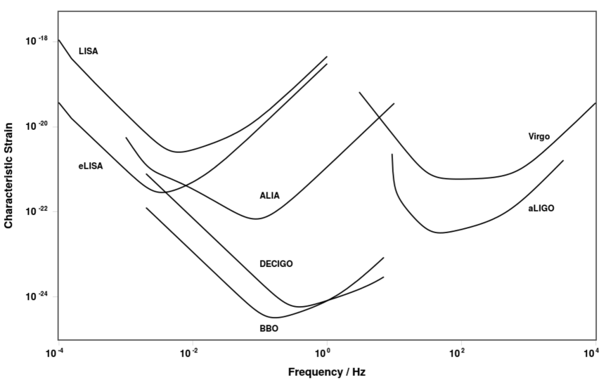
Figure 2: Sensitivities of second generation space and ground-based gravitational wave detectors, in the neutron star spin-frequency range. The sensitivity curves have been generated using publicly available resources at http://www.rhcole.com/apps/GWplotter/ Moore et al. (2015).

The spin-periods of neutron stars (from ultra-fast millisecond pulsars to slow X-ray pulsars in HMXBs) span a range of $10^{-3}-10^{3}$ s. Hence, the detectors appropriate for detecting gravitational wave signatures (of the kind discussed here) would be the aLIGO Abadie et al. (2010) and its extended version once LIGO-India Unnikrishnan (2013) starts operation. But it can also be readily seen that the possibility of detection would be severely limited by the sensitivity of the present day detectors Abbott et al. (2009). However, it can be seen from Fig.[2] that the space-based detectors, like - the evolving Laser Interferometer Space Antenna (eLISA) Consortium et al. (2013), Advanced Laser Interferometer Antenna (ALIA), Big Bang Observer (BBO) and Deci-hertz Interferometer GW Observatory (DECIGO) Moore et al. (2015), would be very good candidates for this kind of work as these would have much higher sensitivities in a range of frequencies that is of interest in the present context. In particular, the frequency range relevant for neutron stars residing in HMXBs ($\nu\sim 10^{-3}-1$ Hz) is precisely the one in which these space-based detectors would be operative, as can be seen from Fig.[2] and Fig.[3].

It is then interesting to find the parameter space (in terms of the spin and the magnetic field of the neutron stars) that is most likely to be sampled by future detectors. Let us assume the neutron stars, in consideration, to have : $M_{\rm ns}=1.4~{}\mbox{{\rm M}${}_{\odot}$},R_{\rm ns}=10~{}{\rm Km}$, accreting at the Eddington rate and at a distance of 1 Kpc. Then from Eq.[18] we obtain,

$$h_{0}=1.87\times 10^{-35}P_{s}^{-2}\left(\frac{B_{s}}{10^{12}~{}G}\right)^{10/7}.$$ (22)

This gives rise to a relation between $P_{s}$ and $B_{s}$ for a given value of $h_{0}$ with the following form,

$$\log_{10}B_{s}=1.4\log_{10}P_{s}+0.7\log_{10}h_{0}+36.31\,,$$ (23)

enabling us to identify the possible region, in the $P_{s}-B_{s}$ plane, where future searches could focus on.

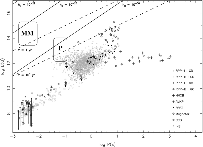
Figure 3: All known neutron stars (for which some measurement/estimate of the magnetic field exists) in the $P_{s}-B_{s}$ plane (a detailed discussion on various observational classes of neutron stars can be found in Konar et al. (2016)). The solid lines marked ‘$h_{0}=10^{-22}$’, ‘$h_{0}=10^{-25}$’ and ‘$h_{0}=10^{-30}$’ are drawn using Eq.[23]. The dashed lines mark spin-down timescales of 1 year and $10^{4}$ years. The rectangle marked ‘MM’ is the region where millisecond magnetars are expected to appear, and the region marked ‘P’ is where non-recycled neutron stars with strong magnetic fields and short spin-periods should be seen.
Legends : RPP - rotation powered pulsar, I/B - isolated/binary, GC - globular cluster, GD - galactic disc, AMXP - accreting millisecond X-ray pulsar (in LMXBs), RRAT - Rotating Radio Transients, INS - isolated neutron star, CCO - central compact object. Note that the vertical lines associated with the AMXPs are uncertainties coming from different models of field estimate, not error bars.
Data : RPP - Manchester et al. (2005), http://www.atnf.csiro.au/research/pulsar/psrcat/;
RRAT - http://astro.phys.wvu.edu/rratalog/;
Magnetar - http://www.physics.mcgill.ca/$\sim$pulsar/magnetar/main.html;
AMXP - Patruno and Watts (2012); Mukherjee et al. (2015); HMXB - Caballero and Wilms (2012); INS - Haberl (2007); Kaplan and van Kerkwijk (2009); CCO - Halpern and Gotthelf (2010); Ho (2013).

In Fig.[3] we plot all known neutron stars (accreting or otherwise) in the $P_{s}-B_{s}$ plane. Lines corresponding to three values of $h_{0}$ have also been indicated in this plot using Eq.[23]. Since the maximum sensitivity limits for aLIGO and BBO are $10^{-22}$ and $10^{-25}$ respectively, the lines corresponding to those values of $h_{0}$ indicate the maximal capabilities of these detectors. Though it must be remembered that such connection to a given detector is purely ‘symbolic’ here as BBO would not even be operative in the indicated frequency range. Therefore, the region to the left of a given line could simply be taken to be indicative of the region of possible detectability (by ‘a’ detector) of gravitational waves with amplitudes equal to or larger than the particular value of $h_{0}$, if it is operative in that frequency. Evidently, no known neutron star inhabits this region. Moreover, all the accreting neutron stars are very far away - the LMXBs being concentrated in the lower left hand and the HMXBs showing up in the upper middle to upper left hand region of the neutron star parameter space.

Looking at Eq.18 or its simplified version Eq.22, it is evident that the amplitude of the emitted gravitational waves increase with a decrease in the spin-period or an increase in the magnetic field of the neutron star. Clearly, rapidly rotating magnetars residing in HMXBs would fit the bill perfectly. It would also not be remiss to note that to generate the strong magnetic fields through a dynamo process, the magnetars are expected to be born rotating fast, with $P\raisebox{-1.29167pt}{\mbox{$\stackrel{{\scriptstyle<}}{{{}_{\sim}}}\,$}}1$ ms Thompson and Duncan (1993). In fact, such objects (nicknamed ‘millisecond magnetars’) have been invoked to explain some of the ultra-luminous soft gamma-ray bursts Lü and Zhang (2014). However, such objects have an extremely rapid rate of spin-down. Assuming the spin-down to be entirely electromagnetic, the characteristic spin-down timescale is given by Zhang and Mészáros (2001),

$$\tau\sim 2\times 10^{3}{\rm s}(I_{45}R_{6}^{-6})B_{s,15}^{-2}P_{s,-3}^{2},$$ (24)

where $I_{45}$, $R_{6}$, $B_{s,15}$ and $P_{s,-3}$ denote the moment of inertia in $10^{45}$ gm.cm², radius in $10^{6}$ cm, $B_{s}$ in $10^{15}$ G and $P_{s}$ in $10^{-3}$ s respectively. In Fig.[3], two dashed lines mark spin-down timescales of 1 year and $10^{4}$ years respectively. Objects on the left of a particular line would have spin-down timescales smaller than that on the line itself. Evidently, the ‘millisecond magnetar’ phase (region marked ‘MM’) would be extremely short-lived.

Nevertheless, strongly magnetised neutron stars residing in HMXBs would still be the best candidates for gravitational waves generated due to the mass quadrupole moments induced by accretion columns, as can be seen from the proximity of magnetars to the $h_{0}=10^{-30}$ line in Fig.[3] (though this is orders of magnitude beyond the detection limit of even the second generation of detectors). Presence of magnetars in HMXBs have recently been invoked to explain certain ultra-luminous super-giant fast X-ray transients Bozzo et al. (2008); Mushtukov et al. (2015). Therefore, such a population, in fact, does exist. Now, it can also be seen from Fig.[3] that the slow magnetars have spin-down timescales $\sim 10^{4}$ years which also happens to be the typical timescale of HMXB activity.

However, it appears that the objects in the region marked ‘P’, neutron stars with reasonably short $P_{s}$ and moderately high $B_{s}$, would be the best candidates (as sources of steady gravitational waves) if they can be found in HMXBs before significant spin-down has happened. Now, we expect to see an order of magnitude increase in the number of radio pulsar detection with the advent of the SKA Smits et al. (2009, 2011). It is conceivable that the region marked ‘P’ may also see an increase in the density of objects with short $P_{s}$ and high $B_{s}$. Detection of early HMXB phase for such neutron stars may happen with the next generation of sensitive X-ray instruments. Consequently, the third generation of space-based detectors would likely be able to target and study steady gravitational waves from such systems.

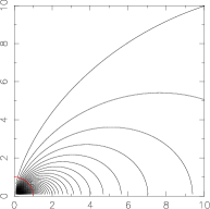
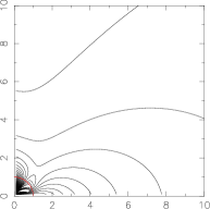
Figure 4: The left-hand panel shows a star-centred dipole field in the range $0\leq\theta\leq\pi/2$. The circular arc denotes the extent of the stellar surface. The plot shows the field lines up-to a distance of 10 stellar radius. In the right-hand panel an off-axis (offset by 60^∘) quadrupole field, twice as strong as the dipole field, has been added.

It should be mentioned here that in the above calculation we have assumed a symmetric dipolar magnetic field. But a complex field with very strong higher multipole components near the surface is not ruled out Gil and Mitra (2001), as shown in Fig.[4]. It is evident that a simple higher multipole component over and above the dipole can create other asymmetric, off-axis polar regions. Charged particles moving along the field lines would create ‘mountains’ at these positions too. Therefore with a complicated magnetic field it is possible to obtain a number of very asymmetric mountains. And if the higher multipole components are much stronger than the dipole then the mass content of the accretion column could be much larger. Recent investigations have shown that higher multipoles can generate large ellipticity and be good candidates for gravitational waves Mastrano et al. (2013).

Moreover, the estimates in this section has implicitly assumed that the accretion-induced mountains would be stable even with surface magnetic fields much larger than $\sim 10^{13}$ G. This assumption may not hold if MHD instabilities become stronger. In that case, the mass content of the accretion induced mountains and the consequent amplitude of the gravitational waves would be even smaller. But a precise statement in this regard can not be made without detailed calculation of accretion onto strongly magnetised neutron stars.

IV conclusion

In this note we present simple estimates of mass quadrupole moments and corresponding amplitudes of the gravitational waves that can be generated by a pair of magnetically confined accretion column. It is seen that the wave amplitudes are too small for the present generation of detectors. However, rapidly rotating strongly magnetised neutron stars in HMXBs are expected to be good candidates for targeted search for gravitational waves by the next generation of detectors.