Phaseless quantum Monte-Carlo approach to strongly correlated superconductors with stochastic Hartree-Fock-Bogoliubov wavefunctions

Abstract

The so-called phaseless quantum Monte-Carlo method currently offers one of the best performing theoretical framework to investigate interacting Fermi systems. It allows to extract an approximate ground-state wavefunction by averaging independent-particle states undergoing a Brownian motion in imaginary-time. Here, we extend the approach to a random walk in the space of Hartree-Fock-Bogoliubov (HFB) vacua that are better suited for superconducting or superfluid systems. Well-controlled statistical errors are ensured by constraining stochastic paths with the help of a trial wavefunction. It also guides the dynamics and takes the form of a linear combination of HFB ansätze. Estimates for the observables are reconstructed through an extension of Wick’s theorem to matrix elements between HFB product states. The usual combinatory complexity associated to the application of this theorem for four- and more- body operators is bypassed with a compact expression in terms of Pfaffians. The limiting case of a stochastic motion within Slater determinants but guided with HFB trial wavefunctions is also considered. Finally, exploratory results for the spin-polarized Hubbard model in the attractive regime are presented.

1 Introduction

Frictionless flow is one of the most spectacular manifestation of quantum coherence in many-body systems at the macroscopic scale. Historically, its appearance in fermion matter has been first evidenced in superconducting (SC) metals, nuclei and superfluid ³He. Currently, Cooper-pair condensates keep on attracting interest, especially because of the diversity of observed ground states. For a large class of SC materials, ranging from elements (such as Hg [1]) to alloys (such as Nb₃Ge [2]), and possibly to the newly discovered high-$T_{c}$ hydrogen sulfide under pressure [3], the pair wavefunction exhibits $s$-wave symmetry. The microscopic mechanism for electron pairing is then well established and invokes a phonon mediated attraction according to Bardeen-Cooper-Schrieffer (BCS) and Eliashberg theories. However, condensed matter physics also harbors an ever increasing family of superconductors that challenges this conventional paradigm. This applies in particular to heavy fermion systems, where the formation of local Cooper pairs is suppressed by the Coulomb interaction. As reviewed by, e.g., Thalmeier et al. [4], this leads to a wealth of behaviors. For example, SC pairing due to magnetic excitons has been observed in UPd₂Al₃ [5]. Alternatively, comprehensive experimental work demonstrated that in several Ce-based systems, including CeCu₂Si₂, SC tends to mostly appear in the vicinity of a quantum critical point [6, 7], thereby providing strong evidence of the interplay between magnetic and pairing degrees of freedom.

Strong correlation is also a hallmark of the superconducting cuprates, where numerous experiments point towards an SC order parameter with $d$-wave symmetry. Furthermore, it has long been suspected on theoretical grounds, that unconventional SC pairing mechanism involving momentum-carrying Cooper pairs is favored in striped phases [8, 9]. The recent observation of pair-density waves in Bi₂Sr₂CaCu₂O_8+x [10] came to support this scenario, that strongly suggests an intertwining of the spin, charge, and pair degrees of freedom [11, 12]. More generally, the SC correlations in cuprates develop from a bad metal normal phase and in the vicinity of an antiferromagnetic order. A similar feature is in fact shared by other classes of high-$T_{c}$ SC compounds, such as iron pnictides and chalcogenides [13]. These materials are nevertheless singular by exhibiting multi-band Fermi surfaces, leading to a non-universal and still under debate SC order parameter where extended $s$-wave and $d$-wave pairing symmetries are close competitors. Finally, ruthenate superconductors currently attract a particular attention due to a spin-triplet $p$-wave pair condensation, possibly induced by ferromagnetic spin fluctuations. In addition, a variety of experiments point toward a chiral SC order parameter that could support non-Abelian excitations [14].

Understanding most of the above mentioned strongly correlated SC systems obviously requires going beyond the standard BCS mean-field approximation that assumes independent Bogoliubov quasiparticles. For lattice electron models, such as the single- or multi-band Hubbard Hamiltonians, Gutzwiller-BCS wavefunctions are thus frequently used as trial states. In this case, strong electronic correlations are included by partially or totally suppressing double occupancy entailed in a BCS ansatz with an assumed internal structure of the fermion pairs [15, 16]. Alternatively, the variational optimization of large coherent superpositions of general BCS states, free of any a priori input on the relevant correlations, have been recently reported [12]. However, Quantum Monte-Carlo (QMC) methods remain indubitably the most powerful approaches to solve the Schrödinger equation in many-body systems. The acronym QMC actually embraces a multitude of stochastic algorithms, but the general strategy is to represent the zero- or finite-temperature equilibrium state as an integral in a high-dimensional space that can be evaluated using random walks. A compelling example is the auxiliary-field QMC approach that performs projection on exact ground states by sampling fictitious systems of independent particles in external fluctuating fields. The half-filled Hubbard model on bipartite lattices has been extensively investigated through such techniques [17, 18]. For instance, the Mott metal-to-insulator transition on the honeycomb lattice was recently addressed on clusters which size exceeds 2000 sites [19, 20]. Another investigated issue is the entanglement of Mott insulators through the determination of the Renyi entropies [21, 22].

Unfortunately, the general applicability of fermionic QMC schemes suffers from the emergence of negative “weights” or even complex contributions, that deteriorate the stochastic reconstruction of the exact wavefunction to a point where the signal-to-noise ratio becomes almost zero. This infamous sign or phase problem has been proven to be NP-hard and its algorithmic solution with polynomial-time complexity probably does not exist [23]. For QMC methods in the configuration space [24, 25, 26] and time-invariant Hamiltonians, a solution could be found in principle by preventing the random walk to move across a node of the exact ground state. In practice, the nodal surface is imposed from a trial wavefunction and calculations become variational. With auxiliary-field QMC approaches, sufficient conditions for the absence of sign/phase problems are known [27]. Otherwise, restricted-path approximations have been developed for lattice models with Hubbard-like Hamiltonians that also ensure a sampling of real Slater determinants [28, 29]. The so-called phaseless QMC scheme developed by Zhang and Krakauer [30] finally provides the most general framework to obtain an approximate ground state of any fermion system defined either by a model or by a realistic Hamiltonian including two-body interactions. In the original formulation, the method relies on a random walk within independent-particle states that is guided and constrained to control phase problems thanks to a trial many-body wavefunction. Up to now, single- or multi-determinant states have been used for this purpose.

In the present paper, we propose an extension better suited for superconductors through BCS wavefunctions not only as trial states, but also as walkers to absorb in a single path fermion-pair condensation. We first review in Section 2 the basic properties of the most general pair coherent states, known as Hartree-Fock-Bogoliubov (HFB) wavefunctions and for which relevant Cooper pairs do not need to be assumed. The imaginary-time many-body Schrödinger equation is then reformulated in Section 3 as the average of stochastic trajectories of such HFB states. The restricted-path approximations required to set up a viable QMC scheme, i.e. free of phase problems and with an ensured finite-variance sampling, are presented in Section 4. The estimation of ground-state observables is discussed in Section 5 by extending the usual Wick theorem to matrix elements between HFB states. Section 6 aims at illustrating the approach and provides a first numerical implementation for a spin-polarized Fermi system in the strongly attractive regime. The last section is devoted to conclusions and perspectives.

All along this work, we consider a general system of fermions interacting via a two-body potential. The associated Hamiltonian will therefore be given, in second quantization, by

$$\hat{H}=\sum_{i,j}h_{i,j}\hat{c}^{\dagger}_{i}\hat{c}^{\vphantom{dagger}}_{j}+\frac{1}{2}\sum_{i,j,k,l}V_{i,j,k,l}\hat{c}^{\dagger}_{i}\hat{c}^{\dagger}_{j}\hat{c}^{\vphantom{dagger}}_{l}\hat{c}^{\vphantom{dagger}}_{k}\,.$$ (1)

$\hat{c}^{\dagger}_{i}$ and $\hat{c}^{\vphantom{dagger}}_{i}$ are the usual creation and annihilation operators of a fermion in the state ${|i\rangle}$ belonging to an orthonormal basis in the one-body space $\mathcal{H}^{(1)}$, which is supposed to be of finite size $d$.

$$h_{i,j}={\langle i|\hat{h}|j\rangle},$$

$$V_{i,j,k,l}={\langle i|\otimes{\langle j|\hat{V}|k\rangle}\otimes|l\rangle},$$ (2)

represent respectively the matrix elements of the one-body Hamiltonian and the binary interactions. In the context of a multiband Hubbard model, $i$ stands for a combined site, spin and orbital index.

2 The manifold of HFB wavefunctions

All zero-temperature QMC methods rely on a numerical reconstruction of the ground state using a stochastic exploration of a basis. For example, the “Diffusion Monte-Carlo” [24, 25, 26, 31] method uses the orthonormal basis of the position representation, which is sampled by means of a random walk or through a Brownian motion associated to the kinetic energy. Alternatively, auxiliary-field QMC approaches, which we will consider in the following, traditionally call upon the overcomplete basis of independent-particle states for a system of $N$ fermions

$${|\Phi\rangle}=\prod_{n=1}^{N}\hat{c}^{\dagger}_{\phi_{n}}{|\,\rangle},\,\,\,\mbox{with}\,\,\,\hat{c}^{\dagger}_{\phi_{n}}=\sum_{i}\hat{c}^{\dagger}_{i}\phi_{i,n}\,.$$ (3)

Here, $\{\phi_{i,n}\}$ denote the components in the basis $\{{|i\rangle}\}$ of individual occupied and orthonormal states. In this work, we propose to extend the formalism to the most general factorized fermionic states, i.e. Hartree-Fock-Bogoliubov (HFB) wavefunctions [32, 33] —also known in condensed-matter Physics as Bogoliubov-de Gennes wavefunctions—,

$${|\Phi\rangle}\propto\prod_{n=1}^{d}\hat{\gamma}_{n}{|\,\rangle}\,,$$ (4)

where the quasiparticle operators $\hat{\gamma}_{n}$ $(n\in\{1,\ldots,d\})$ obey the Fermi-Dirac statistics and are linearly related to the original creation/annihilation fermionic operators

$$\hat{\gamma}_{n}=\sum_{i}\hat{c}_{i}^{\dagger}V^{*}_{i,n}+\hat{c}_{i}^{\vphantom{\dagger}}U^{*}_{i,n},$$ (5)

that is

$$\left(\begin{array}[]{l}\hat{\gamma}\\ \hat{\gamma}^{\dagger}\end{array}\right)=\left(\begin{array}[]{cc}U^{\dagger}&V^{\dagger}\\ V^{T}&U^{T}\end{array}\right)\left(\begin{array}[]{l}\hat{c}\\ \hat{c}^{\dagger}\end{array}\right)\equiv\mathcal{B}^{\dagger}\left(\begin{array}[]{l}\hat{c}\\ \hat{c}^{\dagger}\end{array}\right).$$ (6)

Thus, $\hat{\gamma}_{n}{|\Phi\rangle}=0$ and the HFB state appears as a quasiparticle vacuum. The Bogoliubov transformation matrix $\mathcal{B}$ (6) will moreover be supposed unitary to ensure canonical anticommutation relations $[\hat{\gamma}^{\vphantom{\dagger}}_{n},\hat{\gamma}^{\vphantom{\dagger}}_{p}]_{+}=0$, $[\hat{\gamma}^{\vphantom{\dagger}}_{n},\hat{\gamma}^{\dagger}_{p}]_{+}=\delta_{n,p}\hat{\mathbb{I}}$, and to allow the expansion of the physical operators in terms of quasiparticles

$$\left(\begin{array}[]{l}\hat{c}\\ \hat{c}^{\dagger}\end{array}\right)=\left(\begin{array}[]{cc}U&V^{*}\\ V&U^{*}\end{array}\right)\left(\begin{array}[]{l}\hat{\gamma}\\ \hat{\gamma}^{\dagger}\end{array}\right),$$ (7)

or, equivalently

$$\hat{c}_{i}=\sum_{n}\left(U^{\vphantom{*}}_{i,n}\hat{\gamma}^{\vphantom{\dagger}}_{n}+V^{*}_{i,n}\hat{\gamma}^{\dagger}_{n}\right).$$ (8)

Mathematically, the HFB wavefunctions (4) form an overcomplete set of the Fock space due to their quality of coherent states associated to the Lie algebra $SO(2d)$ of operators $\hat{c}^{\dagger}_{i}\hat{c}^{\vphantom{\dagger}}_{j}-\frac{1}{2}\delta_{i,j}$, $\hat{c}^{\dagger}_{i}\hat{c}^{\dagger}_{j}$, and $\hat{c}^{\vphantom{\dagger}}_{i}\hat{c}^{\vphantom{\dagger}}_{j}$ [34]. As a consequence, every correlated state of a fermionic system can be reconstructed as a linear combination of non-orthogonal HFB wavefunctions. By breaking the $U(1)$ gauge symmetry of the Hamiltonian (1), HFB states physically present the advantage of immediately leading to pairing correlations. A single HFB wavefunction may display the generic properties of superconducting or superfluid fermionic phases, while large coherent superpositions are required to reproduce such behaviors with independent-particle states.

Historically, the condensation of Cooper pairs is however rather apprehended through the BCS wavefunction expressed in terms of couples $\left({|\phi_{\alpha}\rangle},{|\phi_{\tilde{\alpha}}\rangle}\right)$ of one-body states between which pairing is established, and which form an orthonormal basis of $\mathcal{H}^{(1)}$

$${|\Phi^{({\rm BCS})}\rangle}=\prod_{\alpha=1}^{d/2}\left(u_{\alpha}+v_{\alpha}\hat{c}^{\dagger}_{\phi_{\alpha}}\hat{c}^{\dagger}_{\phi_{\tilde{\alpha}}}\right){|\,\rangle}.$$ (9)

$u_{\alpha}$ and $v_{\alpha}$ represent the probability amplitudes for the couple $\left({|\phi_{\alpha}\rangle},{|\phi_{\tilde{\alpha}}\rangle}\right)$ to be unoccupied or populated, respectively. In variational treatments, the BCS mean-field method is based on the minimization of the energy in the state (9) with respect to the parameters $(u_{\alpha},v_{\alpha})$, the pairs $\hat{c}^{\dagger}_{\phi_{\alpha}}\hat{c}^{\dagger}_{\phi_{\tilde{\alpha}}}$ being chosen on physical considerations. The HFB ansatz (4) actually has the advantage of completing the description by determining the optimal basis $\left({|\phi_{\alpha}\rangle},{|\phi_{\tilde{\alpha}}\rangle}\right)$. It may indeed be re-written in a BCS form with states $\left({|\phi_{\alpha}\rangle},{|\phi_{\tilde{\alpha}}\rangle}\right)$ directly encoded in the Bogoliubov transformation. The evidence of this result is based on the Bloch-Messiah-Zumino theorem [35, 36], which states that there exists unitary matrices $C$ and $D$ such that

$$D^{\dagger}UC^{\dagger} =\left(\begin{array}[]{llll}\underline{U}_{1}&0_{2\times 2}&\ldots&0_{2\times 2}\\ 0_{2\times 2}&\underline{U}_{2}&\ldots&0_{2\times 2}\\ \vdots&\vdots&\ddots&\vdots\\ 0_{2\times 2}&0_{2\times 2}&\ldots&\underline{U}_{d/2}\end{array}\right)\equiv\underline{U},$$ (14)

$$D^{T}VC^{\dagger} =\left(\begin{array}[]{llll}\underline{V}_{1}&0_{2\times 2}&\ldots&0_{2\times 2}\\ 0_{2\times 2}&\underline{V}_{2}&\ldots&0_{2\times 2}\\ \vdots&\vdots&\ddots&\vdots\\ 0_{2\times 2}&0_{2\times 2}&\ldots&\underline{V}_{d/2}\end{array}\right)\equiv\underline{V},$$ (19)

where the $2\times 2$ diagonal blocks $\underline{U}_{\alpha}$ and $\underline{V}_{\alpha}$ $(\alpha\in\{1,\ldots,d/2\})$ are respectively characterized by two real positive numbers $u_{\alpha},v_{\alpha}$, and are given by

$$\underline{U}_{\alpha}=\left(\begin{array}[]{cc}u_{\alpha}&0\\ 0&u_{\alpha}\end{array}\right),\quad\underline{V}_{\alpha}=\left(\begin{array}[]{cc}0&v_{\alpha}\\ -v_{\alpha}&0\end{array}\right)\,.$$ (20)

One can then define the orthonormal basis $\left({|\phi_{\alpha}\rangle},{|\phi_{\tilde{\alpha}}\rangle}\right)$ as the one obtained by applying the unitary transformation $D$ on the family ${|i\rangle}$,

$${|\phi_{\alpha}\rangle}=\sum_{i}{|i\rangle}D_{i,2\alpha-1}\,,\quad{|\phi_{\tilde{\alpha}}\rangle}=\sum_{i}{|i\rangle}D_{i,2\alpha}.$$ (21)

Through the previous decomposition of the matrices $U$ and $V$ in their respective canonical form $\underline{U}$ and $\underline{V}$, the quasiparticle operators $\hat{\gamma}_{n}$ (5) of the HFB state can be immediately obtained in terms of their counterparts $\underline{\hat{\gamma}}_{\alpha}=u_{\alpha}\hat{c}^{\vphantom{\dagger}}_{\phi_{\alpha}}-v_{\alpha}\hat{c}^{\dagger}_{\phi_{\tilde{\alpha}}}$, $\underline{\hat{\gamma}}_{\tilde{\alpha}}=u_{\alpha}\hat{c}^{\vphantom{\dagger}}_{\phi_{\tilde{\alpha}}}+v_{\alpha}\hat{c}^{\dagger}_{\phi_{\alpha}}$ for the BCS wavefunction (9)

$$\hat{\gamma}^{\vphantom{\dagger}}_{n}=\sum_{\alpha=1}^{d/2}\left(\underline{\hat{\gamma}}^{\vphantom{\dagger}}_{\alpha}C^{*}_{2\alpha-1,n}+\underline{\hat{\gamma}}^{\vphantom{\dagger}}_{\tilde{\alpha}}C^{*}_{2\alpha,n}\right)\,.$$ (22)

Taking into account the commutative algebra of the different factors, one is led to

$$\prod_{n=1}^{d}\hat{\gamma}_{n}{|\,\rangle}=\det\left(C^{*}\right)\prod_{\alpha=1}^{d/2}\underline{\hat{\gamma}}_{\alpha}\underline{\hat{\tilde{\gamma}}}_{\alpha}{|\,\rangle}\,.$$ (23)

In addition, all products $\underline{\hat{\gamma}}^{\vphantom{\dagger}}_{\alpha}\underline{\hat{\gamma}}^{\vphantom{\dagger}}_{\tilde{\alpha}}$ commute and the action of each of them on the vacuum is equivalent to $u_{\alpha}v_{\alpha}\hat{c}^{\vphantom{\dagger}}_{\phi_{\alpha}}\hat{c}^{\dagger}_{\phi_{\tilde{\alpha}}}$ or $u_{\alpha}v_{\alpha}\hat{\mathbb{I}}+v_{\alpha}^{2}\hat{c}^{\dagger}_{\phi_{\alpha}}\hat{c}^{\dagger}_{\phi_{\tilde{\alpha}}}$. When setting

$${|\Phi\rangle}=\frac{1}{\nu_{1}\ldots\nu_{d/2}}\hat{\gamma}_{1}\ldots\hat{\gamma}_{d}{|\,\rangle}\,,$$ (24)

the HFB state finally reduces, up to a phase factor $\det(C^{*})$, to a BCS ansatz with pairs directly stemming from the Bogoliubov transformation. From now on, we will adopt this form which clarifies the normalization constant in the definition (4).

In the following, the manipulation of quasiparticle operators (5) will be greatly facilitated by adding a label $\varpi\in\{p,h\}$ to each individual state, that indicates whether it refers to a particle ($p$) or to a hole ($h$). In other words, we define $\hat{c}_{pi}^{\dagger}=\hat{c}_{i}^{\dagger}$ and $\hat{c}_{hi}^{\dagger}=\hat{c}_{i}^{\vphantom{\dagger}}$. The extended one-body space obtained this way identifies to the tensor product $\mathcal{H}_{ex}^{(1)}=\mathcal{H}^{(ph)}\otimes\mathcal{H}^{(1)}$, where $\mathcal{H}^{(ph)}$ refers to the abstract space of dimension two underpinned by an orthonormal basis $\{{|e_{p}\rangle},{|e_{h}\rangle}\}$ related to the two flavors “particle”, “hole”. In this context, we can for example immediately check that the unitary character of the Bogoliubov matrix is equivalent to providing the extended space with an orthonormal basis built upon the vectors

$${|\gamma_{n}\rangle}=\left(\begin{array}[]{l}{|V^{*}_{n}\rangle}\\ {|U^{*}_{n}\rangle}\end{array}\right),\,{|\bar{\gamma}_{n}\rangle}=\left(\begin{array}[]{l}{|U_{n}\rangle}\\ {|V_{n}\rangle}\end{array}\right),$$ (25)

where ${|U_{n}\rangle}=\sum_{i}{|i\rangle}U_{i,n}$, ${|U^{*}_{n}\rangle}=\sum_{i}{|i\rangle}U^{*}_{i,n}$ (as well as ${|V_{n}\rangle}$ and ${|V^{*}_{n}\rangle}$) are defined from the amplitudes of the transformation. Indeed,

$$\sum_{n=1}^{d}\left({|\gamma_{n}\rangle}\langle\gamma_{n}|+{|\bar{\gamma}_{n}\rangle}\langle\bar{\gamma}_{n}|\right)=\mathbb{I}\,,\,\,\,\left\{\begin{array}[]{l}{\langle\gamma_{n}|\gamma_{p}\rangle}={\langle\bar{\gamma}_{n}|\bar{\gamma}_{p}\rangle}=\delta_{n,p}\\ {\langle\gamma_{n}|\bar{\gamma}_{p}\rangle}=0\end{array}\right.\,.$$ (26)

In addition, the relations (6, 7) between the fermionic operators and the quasiparticles are simply written as

$$\left\{\begin{array}[]{l}\hat{\gamma}_{n}=\sum_{\varpi i}\hat{c}_{\varpi i}^{\dagger}{\langle\varpi i|\gamma_{n}\rangle}=\sum_{\varpi i}{\langle\bar{\gamma}_{n}|\varpi i\rangle}\hat{c}_{\varpi i}^{\vphantom{\dagger}}\\ \hat{\gamma}_{n}^{\dagger}=\sum_{\varpi i}\hat{c}_{\varpi i}^{\dagger}{\langle\varpi i|\bar{\gamma}_{n}\rangle}=\sum_{\varpi i}{\langle\gamma_{n}|\varpi i\rangle}\hat{c}_{\varpi i}^{\vphantom{\dagger}}\end{array}\right.,$$ (27)

and

$$\left\{\begin{array}[]{l}\hat{c}_{\varpi i}^{\vphantom{\dagger}}=\sum_{n=1}^{d}\left({\langle\varpi i|\bar{\gamma}_{n}\rangle}\hat{\gamma}_{n}+{\langle\varpi i|\gamma_{n}\rangle}\hat{\gamma}_{n}^{\dagger}\right)\\ \hat{c}_{\varpi i}^{\dagger}=\sum_{n=1}^{d}\left(\hat{\gamma}_{n}{\langle\gamma_{n}|\varpi i\rangle}+\hat{\gamma}_{n}^{\dagger}{\langle\bar{\gamma}_{n}|\varpi i\rangle}\right)\end{array}\right..$$ (28)

These expansions show that the operator $\hat{\gamma}_{n}$ depends linearly on the ket ${|\gamma_{n}\rangle}$ or on the bra $\langle\bar{\gamma}_{n}|$. Accordingly, his adjoint $\hat{\gamma}_{n}^{\dagger}$ is a linear function of the ket ${|\bar{\gamma}_{n}\rangle}$ or of the bra $\langle\gamma_{n}|$.

3 Stochastic reformulation of the imaginary-time dependent Schrödinger equation with HFB walkers

Auxiliary-field QMC approaches are based on the dynamics in imaginary time of an initial wavefunction ${|\Phi_{0}\rangle}$ in order to project it onto the ground state ${|\Psi_{G}\rangle}$ of the Hamiltonian:

$${|\Psi_{G}\rangle}\propto\lim_{\tau\rightarrow\infty}\exp\bigl{(}-\tau\hat{H}\bigr{)}{|\Phi_{0}\rangle}.$$ (29)

One typically chooses ${|\Phi_{0}\rangle}$ as an independent-particle state and, thanks to the Hubbard-Stratonovich transformation [37, 38], the $N$-body propagator $\exp(-\tau\hat{H})$ is rewritten in the form of a multidimensional integral of one-body propagators in fluctuating effective potentials. For fermions, the exact ground state thus appears eventually as an average of Slater determinants ${|\Phi_{\tau}\rangle}$, which individual states follow a Brownian motion and are consequently called walkers

$${|\Psi_{G}\rangle}\propto\lim_{\tau\rightarrow\infty}\mathbb{E}[{|\Phi_{\tau}\rangle}]\,,$$ (30)

in which $\mathbb{E}[\ldots]$ stands for the ensemble average of a stochastic process. Despite its use in most QMC simulations, such a scheme is not the optimal reformulation of the Schrödinger equation in imaginary time for the $N$-body state. Indeed, the broadening of the probability distribution of the walkers, measured through the growth of the averaged quadratic distance

$$\mathbb{E}\Bigl{[}\bigl{|}\bigl{|}\rme^{-\tau\hat{H}}{|\Phi_{0}\rangle}-{|\Phi_{\tau}\rangle}\bigr{|}\bigr{|}^{2}\Bigr{]},$$ (31)

between the exact propagation and one of its stochastic realizations, is not made minimal. A QMC scheme fulfilling such a criterion was identified in 2001 for a system of bosons [39] and extended in 2002 to fermions [40]. It is based on a one-body dynamics controlled by the mean-field Hartree-Fock Hamiltonian and enhanced by one-particle one-hole stochastic excitations. In addition, each realization is separated from the exact state by a bounded distance so that the variance of any observable is guaranteed not to diverge [40]. This method remains delicate to implement numerically and suffers in general, as does the standard scheme, from the usual sign/phase problem. It has essentially been applied to study the development of pairing correlations in a one-dimensional system of cold atoms trapped in a harmonic well or on a rotating torus [41].

In order to improve the efficiency of the standard auxiliary-field QMC dynamics, Zhang & Krakauer suggested to incorporate in the motion of the walkers a complex importance function given by their overlap with a previously chosen trial state ${|\Psi_{T}\rangle}$ not orthogonal to ${|\Psi_{G}\rangle}$ [30]

$${|\Psi_{G}\rangle}\propto\lim_{\tau\rightarrow\infty}\mathbb{E}\left[\Pi_{\tau}\frac{{|\Phi_{\tau}\rangle}}{{\langle\Psi_{T}|\Phi_{\tau}\rangle}}\right].$$ (32)

Here, the addition of the factor $\Pi$ is necessary for the stochastic scheme to be equivalent to the Schrödinger equation in imaginary time, as we will see below. To date, the main applications of the sampling (32) are related to quantum chemistry with a trial state ${|\Psi_{T}\rangle}$ as well as walkers ${|\Phi_{\tau}\rangle}$ being Slater determinants [42]. Frustrated magnetic models have also been apprehended with a similar random walk within matrix-product states [43]. Finally, the approach has been generalized to rebuild, in the context of nuclear structure, the ground state [44] as well as excited states [45] in each symmetry sector of the Hamiltonian via wavefunctions projected onto the related quantum numbers. In the following, we extend the guided dynamics QMC scheme (32) to HFB-type walkers.

Let us first consider the exact propagation of the ansatz ${|W\rangle}=\Pi{|\Phi\rangle}/{\langle\Psi_{T}|\Phi\rangle}$ built from a normalized Bogoliubov vacuum ${|\Phi\rangle}$ (24), an arbitrary test wavefunction ${|\Psi_{T}\rangle}$, and a multiplicative complex variable $\Pi$. After an infinitesimal imaginary time $\rmd\tau$, the Schrödinger equation leads to a correlated state, given to first order in $\rmd\tau$, by

$$\exp\bigl{(}-\rmd\tau\hat{H}\bigr{)}{|W\rangle}={|W\rangle}-\rmd\tau\hat{H}{|W\rangle}.$$ (33)

On the other hand, an elementary variation of ${|W\rangle}$ may be obtained by slightly changing the HFB state by means of a transformation $\hat{T}=\exp\left(\rmd\hat{x}\right)$, where $\rmd\hat{x}$ is a general one-body operator, with infinitesimal matrix elements and which possibly includes terms $\hat{c}_{i}^{\dagger}\hat{c}_{j}^{\dagger}$, $\hat{c}_{i}^{\vphantom{\dagger}}\hat{c}_{j}^{\vphantom{\dagger}}$ that break particle-number conservation. With the notations of the extended space $\mathcal{H}^{(1)}_{\rm ex}$, we have

$$\rmd\hat{x}=\sum_{\varpi i,\varpi^{\prime}j}\rmd x_{\varpi i,\varpi^{\prime}j}\hat{c}_{\varpi i}^{\dagger}\hat{c}_{\varpi^{\prime}j}^{\vphantom{\dagger}}\,.$$ (34)

The operators

$$\hat{\beta}_{n}=\hat{T}\hat{\gamma}_{n}\hat{T}^{-1},$$ (35)

stemming from the transformation of the quasiparticles $\hat{\gamma}_{n}$ of ${|\Phi\rangle}$ are easily obtained from their expansion (27) on the set $\{\hat{c}_{\varpi i}^{\dagger}\}$, the Glauber formula and the following relations inherent to the definitions $\hat{c}_{pi}^{\dagger}=\hat{c}_{i}^{\dagger}$, $\hat{c}_{hi}^{\dagger}=\hat{c}_{i}^{\vphantom{\dagger}}$

$$\bigl{[}\hat{c}_{\varpi i}^{\dagger},\hat{c}_{\varpi^{\prime}j}^{\vphantom{\dagger}}\bigr{]}_{+} =\delta_{\varpi i,\varpi^{\prime}j}\hat{\mathbb{I}},$$

$$\bigl{[}\hat{c}_{\varpi i}^{\vphantom{\dagger}},\hat{c}_{\varpi^{\prime}j}^{\vphantom{\dagger}}\bigr{]}_{+} =\sigma_{\varpi i,\varpi^{\prime}j}\hat{\mathbb{I}},$$ (36)

where

$$\sigma=\left(\begin{array}[]{cc}0_{d\times d}&\mathbb{I}_{d\times d}\\ \mathbb{I}_{d\times d}&0_{d\times d}\end{array}\right)\,\,\ \mbox{so that}\,\,\,\hat{c}_{\varpi i}^{\vphantom{\dagger}}=\sum_{\varpi^{\prime}j}\sigma_{\varpi i,\varpi^{\prime}j}\hat{c}_{\varpi^{\prime}j}^{\dagger}\,.$$ (37)

Ultimately, $\hat{\beta}_{n}$ remains linearly related to fermionic creation/annihilation operators with an associated vector in $\mathcal{H}^{(1)}_{\rm ex}$ given by

$${|\beta_{n}\rangle}=\exp\bigl{(}\rmd x-\sigma\rmd x^{T}\sigma\bigr{)}{|\gamma_{n}\rangle}.$$ (38)

Since the operator $\hat{T}$ is not necessarily unitary, the kets ${|\beta_{n}\rangle}$ do not generally form an orthonormal family. However, they remain orthogonal to all their partners ${|\bar{\beta}_{n}\rangle}=\sigma{|\beta_{n}^{*}\rangle}$ generated by complex conjugation followed by the exchange of high and low components

$${\langle\bar{\beta}_{p}|\beta_{n}\rangle}=\bigl{[}\hat{\beta}_{p},\hat{\beta}_{n}\bigr{]}_{+}=\hat{T}\bigl{[}\hat{\gamma}_{p},\hat{\gamma}_{n}\bigr{]}_{+}\hat{T}^{-1}=0$$ (39)

Moreover, the orthonormalization of the vectors ${|\beta_{1}\rangle},\ldots{|\beta_{d}\rangle}$ through linear combinations

$${|\lambda_{n}\rangle}=\sum_{p}\mathcal{O}_{np}{|\beta_{p}\rangle},$$ (40)

automatically induces the orthonormalization of their partners ${|\bar{\lambda}_{n}\rangle}=\sigma{|\lambda^{*}_{n}\rangle}$ belonging to the orthogonal subspace. Indeed,

$${\langle\bar{\lambda}_{n}|\bar{\lambda}_{p}\rangle}={\langle\lambda_{p}|\lambda_{n}\rangle}=\delta_{np}\,\,\,\mbox{and}\,\,\,{|\bar{\lambda}_{n}\rangle}=\sum_{p}\mathcal{O}^{*}_{np}{|\bar{\beta}_{p}\rangle}.$$ (41)

As a consequence, the $2d$ vectors $\{{|\lambda_{n}\rangle},{|\bar{\lambda}_{n}\rangle}\}$ form an orthonormal basis of the extended one-body space and they therefore define a new normalized HFB state ${|\Lambda\rangle}$. In reality, ${|\Lambda\rangle}$ and $\hat{T}{|\Phi\rangle}$ are collinear insofar as they are a vacuum of the same quasiparticles

$$\hat{\lambda}_{n}=\sum_{p}\mathcal{O}_{np}\hat{\beta}_{p},$$

$$\hat{\lambda}_{n}\hat{T}{|\Phi\rangle}=\sum_{p}\mathcal{O}_{np}\hat{T}\hat{\gamma}_{p}{|\Phi\rangle}=0.$$ (42)

It should be noted that the preservation of a quasiparticle product by application of the transformation $\hat{T}$ is not at all elementary for operators $\rmd\hat{x}$ containing contributions of the type $\hat{c}^{\dagger}_{i}\hat{c}^{\dagger}_{j}$. In this case, $\hat{T}$ indeed changes the particle vacuum, whereas if $\rmd\hat{x}{|\,\rangle}=0$, $\hat{T}{|\,\rangle}={|\,\rangle}$, and one immediately has

$$\hat{T}{|\Phi\rangle}\propto\prod_{n=1}^{d}\hat{T}\hat{\gamma}_{n}\hat{T}^{-1}{|\,\rangle}=\prod_{n=1}^{d}\hat{\beta}_{n}{|\,\rangle}=\frac{1}{\mbox{det}\mathcal{O}}\prod_{n=1}^{d}\hat{\lambda}_{n}{|\,\rangle}\propto{|\Lambda\rangle}.$$ (43)

In conclusion, we have shown that the vector $\exp\left(\rmd\hat{x}\right){|\Phi\rangle}$ identifies, up to a multiplicative constant, to a HFB wavefunction ${|\Lambda\rangle}$, that is infinitely close to ${|\Phi\rangle}$, and which quasiparticles are always derived from a unitary canonical transformation of the original fermionic operators $\hat{c}_{i}^{\dagger}$, $\hat{c}_{i}^{\vphantom{\dagger}}$. ${|\Lambda\rangle}$ may therefore be noted ${|\Phi+\rmd\Phi\rangle}$. We are thus immediately able to determine the elementary motion of the ansatz ${|W\rangle}$

$${|W+\rmd W\rangle} =\frac{\Pi+\rmd\Pi}{{\langle\Psi_{T}|\Phi+\rmd\Phi\rangle}}{|\Phi+\rmd\Phi\rangle}$$ (44)

$$=\frac{\Pi+\rmd\Pi}{{\langle\Psi_{T}|\exp\left(\rmd\hat{x}\right)|\Phi\rangle}}\exp\left(\rmd\hat{x}\right){|\Phi\rangle}$$

$$=\biggl{(}1+\frac{\rmd\Pi}{\Pi}-\langle\rmd\hat{x}\rangle_{\Psi_{T},\Phi}-\frac{1}{2}\langle\rmd\hat{x}^{2}\rangle_{\Psi_{T},\Phi}+\langle\rmd\hat{x}\rangle^{2}_{\Psi_{T},\Phi}-\frac{\rmd\Pi}{\Pi}\langle\rmd\hat{x}\rangle_{\Psi_{T},\Phi}+\ldots\biggr{)}{|W\rangle}$$

$$\quad+\biggl{(}1+\frac{\rmd\Pi}{\Pi}-\langle\rmd\hat{x}\rangle_{\Psi_{T},\Phi}+\ldots\biggr{)}\rmd\hat{x}{|W\rangle}$$

$$\quad+\frac{1}{2}\rmd\hat{x}^{2}{|W\rangle}+\ldots$$

Here, only the contributions up to second order have been detailed and the notation $\langle\hat{A}\rangle_{\Psi_{T},\Phi}$ for an operator $\hat{A}$ refers to its local estimator, according to the terminology of the QMC formalisms based on a random walk in real space

$$\langle\hat{A}\rangle_{\Psi_{T},\Phi}=\frac{{\langle\Psi_{T}|\hat{A}|\Phi\rangle}}{{\langle\Psi_{T}|\Phi\rangle}}.$$ (45)

At first glance and by comparison with the exact dynamics (33), the expansion (44) is encouraging, showing one-body and two-body terms applied on the ansatz ${|W\rangle}$. A more striking similarity can be easily obtained by rewriting the Hamiltonian (1) as a quadratic form of general one-body operators (in the sense of the extended space $\mathcal{H}^{(1)}_{\rm ex}$)

$$\hat{H}=\hat{K}-\sum_{s}\omega_{s}\hat{O}^{2}_{s},$$ (46)

with

$$\hat{K} =\sum_{\varpi i,\varpi^{\prime}j}K_{\varpi i,\varpi^{\prime}j}\hat{c}_{\varpi i}^{\dagger}\hat{c}_{\varpi^{\prime}j}^{\vphantom{\dagger}},$$

$$\hat{O}_{s} =\sum_{\varpi i,\varpi^{\prime}j}\left[O_{s}\right]_{\varpi i,\varpi^{\prime}j}\hat{c}_{\varpi i}^{\dagger}\hat{c}_{\varpi^{\prime}j}^{\vphantom{\dagger}}.$$ (47)

Such an expression is immediately obtained by bringing each two-body interaction term $\hat{c}_{i}^{\dagger}\hat{c}_{j}^{\dagger}\hat{c}_{l}^{\vphantom{\dagger}}\hat{c}_{k}^{\vphantom{\dagger}}$ in the one of the forms $\pm\frac{1}{2}\bigl{(}\hat{c}_{i}^{\dagger}\hat{c}_{j}^{\dagger}\pm\hat{c}_{l}^{\vphantom{\dagger}}\hat{c}_{k}^{\vphantom{\dagger}}\bigr{)}{}^{2}$, $\mp\frac{1}{2}\bigl{(}\hat{c}_{i}^{\dagger}\hat{c}_{l}^{\vphantom{\dagger}}\pm\hat{c}_{j}^{\dagger}\hat{c}_{k}^{\vphantom{\dagger}}\bigr{)}{}^{2}$ or $\pm\frac{1}{2}\bigl{(}\hat{c}_{i}^{\dagger}\hat{c}_{k}^{\vphantom{\dagger}}\pm\hat{c}_{j}^{\dagger}\hat{c}_{l}^{\vphantom{\dagger}}\bigr{)}{}^{2}$, that may need to be completed with appropriate one-body terms. We refer to [46, 47] for the construction, from the matrix elements $h_{i,j}$ and $V_{i,j,k,l}$, of decompositions of the Hamiltonian that are less schematic and more efficient for QMC treatments as they require a much lower number of operators $\hat{O}_{s}$. With the expression (46) for $\hat{H}$, the exact dynamics (33) during $\rmd\tau$ is obviously transformed into

$$\exp\bigl{(}-\rmd\tau\hat{H}\bigr{)}{|W\rangle}={|W\rangle}-\rmd\tau\hat{K}{|W\rangle}+\rmd\tau\sum_{s}\omega_{s}\hat{O}^{2}_{s}{|W\rangle}.$$ (48)

Thus, in the presence of two-body interactions, it can not be absorbed by a purely determinist evolution (44) of the ansatz ${|W\rangle}$: Under this assumption, $\rmd\Pi$ and $\rmd\hat{x}$ are proportional to $\rmd\tau$ and it is impossible, to first order in $\rmd\tau$, to get back the quadratic terms of the exact propagation. Only contributions schematically proportional to $\sqrt{\rmd\tau}$ in the operator $\rmd\hat{x}$ are able to achieve this via the term in $\rmd\hat{x}^{2}$ of the expansion (44). However, these contributions will also manifest themselves through one-body contaminations in $\sqrt{\rmd\tau}$ which have no counterpart in the evolution resulting from the Schrödinger equation.

The idea consists in making them fluctuating with a zero average. Mathematically, the goal is to include in $\rmd\hat{x}$ (resp. $\rmd\Pi$) stochastic contributions $\rmd\hat{x}_{\rm stoch}$ (resp. $\rmd\Pi_{\rm stoch}$) that depend linearly on the infinitesimal increments $\{\rmd W_{s}\}$ of independent Wiener’s stochastic processes $\{W_{s}\}$ associated with the operators $\{\hat{O}_{s}\}$ entering in the decomposition (46) of the Hamiltonian. In Itô’s calculus [48], these quantities $\rmd W_{s}$ indeed exhibit the properties

$$\mathbb{E}\left[\rmd W_{s}\right]=0$$

$$\rmd W_{s}\rmd W{}_{s^{\prime}}=\delta_{s,s^{\prime}}\rmd\tau,\,\,\,\forall s,s^{\prime}.$$ (49)

Concretely, their simulation on a small finite time $\Delta\tau$ goes through the introduction of random variables $\eta_{s}$ with zero average and variance unity which allows to access the increments $\Delta W_{s}=\int_{\tau}^{\tau+\rmd\tau}\rmd W_{s}$ using $\Delta W_{s}=\eta_{s}\sqrt{\Delta\tau}$. The variables $\eta_{s}$ are commonly referred to as auxiliary fields and are often generated according to a normal distribution. Therefore, the exact dynamics will be found by averaging the stochastic ansätze ${|W+\rmd W\rangle}$ provided the following conditions are simultaneously verified

$$\frac{\rmd\Pi_{\rm det}}{\Pi}-\langle\rmd\hat{x}_{\rm det}\rangle_{\Psi_{T},\Phi}-\frac{1}{2}\langle\rmd\hat{x}^{2}_{\rm stoch}\rangle_{\Psi_{T},\Phi}+\langle\rmd\hat{x}_{\rm stoch}\rangle^{2}_{\Psi_{T},\Phi}-\frac{\rmd\Pi_{\rm stoch}}{\Pi}\langle\rmd\hat{x}_{\rm stoch}\rangle_{\Psi_{T},\Phi}=0,$$ (50a)

$$\rmd\hat{x}_{\rm det}+\frac{\rmd\Pi_{\rm stoch}}{\Pi}\rmd\hat{x}_{\rm stoch}-\langle\rmd\hat{x}_{\rm stoch}\rangle_{\Psi_{T},\Phi}\rmd\hat{x}_{\rm stoch}=-\rmd\tau\hat{T},$$ (50b)

$$\frac{1}{2}\rmd\hat{x}_{\rm stoch}^{2}=\rmd\tau\sum_{s}\omega_{s}\hat{O}^{2}_{s},$$ (50c)

where $\rmd\hat{x}_{\rm det}$ (resp. $d{\Pi}_{\rm det}$) stands for the determinist terms, proportional to $\rmd\tau$, which form $\rmd\hat{x}$ (resp. $d{\Pi}$). These relations do not uniquely determine the equations of motion for the quasiparticle states and for the prefactor $\Pi$. In view of the properties (3), the last constraint (50c) is satisfied as long as

$$\rmd\hat{x}_{{\rm stoch}}=\sum_{s}\sqrt{2\omega_{s}}\hat{O}_{s}\rmd W_{s}\,.$$ (50ay)

Moreover, by making explicit the linear relation between $\rmd\Pi_{\rm stoch}$ and the increments $\rmd W_{s}$ in the form $\rmd\Pi_{{\rm stoch}}=\Pi\sum_{s}\sqrt{2\omega_{s}}g_{s}\rmd W_{s}$ with arbitrary scalars $g_{s}$, we get successively from the equalities (50a - 50b)

$$\rmd\hat{x}_{\rm det} =-\rmd\tau\left[\hat{T}-2\omega_{s}\langle\hat{O}_{s}-g_{s}\rangle_{\Psi_{T},\Phi}\hat{O}_{s}\right]$$

$$\rmd\Pi_{\rm det} =-\Pi\,\rmd\tau\,\langle\hat{H}\rangle_{\Psi_{T},\Phi}\,.$$ (50az)

Eventually, by iterating the process for each ansatz ${|W+\rmd W\rangle}$ obtained at the end of the propagation during $\rm\rmd\tau$, we are led to a representation (32) of the ground state. The quasiparticles of the HFB vacua ${|\Phi_{\tau}\rangle}$ are defined by the realizations at the imaginary time $\tau\rightarrow\infty$ of a Brownian motion in the extended one-body space, which is directly deduced from equations (38, 50ay, 3, and 40)

$${|\gamma_{n}+d\gamma_{n}\rangle}=\mathcal{O}\biggl{\{}{|\gamma_{n}\rangle} -\rmd\tau\Bigl{[}\tilde{K}-\sum_{s}\omega_{s}\Bigl{(}\tilde{O}^{2}_{s}+2\langle\hat{O}_{s}-g_{s}\rangle_{\Psi_{T},\Phi}\tilde{O}_{s}\Bigl{)}\Bigr{]}{|\gamma_{n}\rangle}\biggr{.}$$

. $$+\sum_{s}\sqrt{2\omega_{s}}\rmd W_{s}\tilde{O}_{s}{|\gamma_{n}\rangle}\biggr{\}}.$$ (50ba)

Here, $\mathcal{O}$ is a formal notation to indicate an orthonormalization process according to the previous discussion and $\tilde{K}=K-\sigma K^{T}\sigma$, $\tilde{O}_{s}=O_{s}-\sigma O^{T}_{s}\sigma$. The prefactor $\Pi$ evolves according to

$$\frac{\rmd\Pi}{\Pi}=-\rmd\tau\langle\hat{H}\rangle_{\Psi_{T},\Phi}+\sum_{s}\sqrt{2\omega_{s}}g_{s}\rmd W_{s}.$$ (50bb)

This stochastic differential equation easily fits into Itô’s formalism and its solution $\Pi_{\tau}$ at time $\tau$ is given by

$$\Pi_{\tau}={\langle\Psi_{T}|\Phi_{0}\rangle}\exp\biggl{\{}-\!\!\int_{0}^{\tau}\!\Bigl{[}\rmd\tau^{\prime}\Bigl{(}\langle\hat{H}\rangle_{\Psi_{T},\Phi_{\tau^{\prime}}}+\sum_{s}\omega_{s}g_{s,\tau^{\prime}}^{2}\Bigr{)}+\sum_{s}\sqrt{2\omega_{s}}g_{s,\tau^{\prime}}\rmd W_{s,\tau^{\prime}}\Bigr{]}\biggr{\}}.$$ (50bc)

The quantities $g_{s}$ thus remain undefined on average by the conditions (50a, 50b, 50c), which sometimes leads to qualify them as “stochastic gauges” [49]. They are however involved in the growth of the averaged quadratic error and thus can affect the efficiency of the sampling. Up to date, no numerical applications involving Slater determinants have taken into account an imaginary-time dependence of the gauges $\{g_{s}\}$, and the choices $g_{s}=0$ or $g_{s}=\langle\hat{O}_{s}\rangle_{\Psi_{T},\Psi_{T}}$ have been proposed [42].

It should be finally noted that the Brownian motion (3, 50bb) of HFB walkers allows to find the usual reconstruction scheme (32) of the ground state with stochastic Slater determinants. Indeed, let us consider such a Hartree-Fock (HF) wavefunction ${|\Phi\rangle}=\prod_{n=1}^{N}\hat{c}^{\dagger}_{\phi_{n}}{|\,\rangle}$ built from $N$ orthonormal one-body states $\{{|\phi_{n}\rangle},n=1,2,\ldots,N\}$. By completing their set with a family of unoccupied vectors $\{{|\bar{\phi}_{\nu}\rangle},\nu=1,\ldots,d-N\}$ to have an orthonormal basis of $\mathcal{H}^{(1)}$, ${|\Phi\rangle}$ appears as a vacuum for the operators $\hat{c}^{\dagger}_{\phi_{n}}$ and $\hat{c}^{\vphantom{\dagger}}_{\bar{\phi}_{\nu}}$ which play the role of quasiparticles $\hat{\gamma}_{1},\ldots,\hat{\gamma}_{d}$. The associated vectors in the extended one-body space $\mathcal{H}^{(1)}_{\rm ex}$ are therefore given by

$${|\gamma_{n}\rangle}=\left(\begin{array}[]{c}{|\phi_{n}\rangle}\\ 0\end{array}\right)\,\,\mbox{for }\,n=1,\ldots,N,\,\,\ \mbox{and }\,\,{|\gamma_{n}\rangle}=\left(\begin{array}[]{c}0\\ {|\bar{\phi}^{*}_{n-N}\rangle}\end{array}\right)\,\,\mbox{for }\,n=N+1,\ldots,d.$$ (50bd)

By solely retaining in the rewriting (46) of the Hamiltonian operators $\hat{O}_{s}$ that conserve the particle number, this structure is preserved by the dynamics (3), which immediately gives the evolution of the occupied states ${|\phi_{n}\rangle}$. The results obtained this way are identical to those presented in the original reference [30] in the limit of a continuous imaginary time. Indeed, the strategy adopted in this work is based on a discretization of the exact propagation which is then reformulated in terms of a random walk via the Hubbard-Stratonovich transformation. The method that we have followed here actually originates from the QMC approaches developed for systems of interacting bosons by stochastic extension of the mean-field approximations [39].

4 Control of the phase and infinite-variance problems

Apart from a few exceptional models, the QMC reconstruction of the ground state ${|\Psi_{G}\rangle}$ suffers from the pathological phase problem (or sign problem when the walkers can be restricted to maintain a wavefunction with real components during their Brownian motion). In practice, this problem manifests itself by an exponential growth, with the time and/or the size of the system, of the statistical error on the averaged value of any observable. Its origin is intimately connected to the principles of quantum physics that set the state vector ${|\Psi_{G}\rangle}$ up to a phase. The probability distribution of walkers being real and positive, it may not be sensitive to this phase and inexorably samples the vectors $\{\rme^{\rmi\Theta_{G}}{|\Psi_{G}\rangle},\Theta_{G}\in\mathbb{R}\}$ which are physically equivalent. From then on, one immediately sees that by averaging all the realizations, regardless of the phase $\Theta_{G}$ to which they lead for the ground state, some mutually cancel each other and alter the efficiency of the reconstruction scheme. The missing access to $\Theta_{G}$ prevents an exact control of this problem, except from a modification of the stochastic dynamics of walkers to ensure an overlap of constant phase with ${|\Psi_{G}\rangle}$.

Let us concretely consider the previously developed QMC scheme (32), that is guided by a trial state ${|\Psi_{T}\rangle}$. Its viability is actually questioned as soon as even the smallest population of realizations ${|W_{\tau^{*}}\rangle}=\Pi_{\tau^{*}}{|\Phi_{\tau^{*}}\rangle}/{\langle\Psi_{T}|\Phi_{\tau^{*}}\rangle}$, which collectively have a zero average overlap with ${|\Psi_{G}\rangle}$, emerges at any given time $\tau^{*}$. Their statistical weight remains however negligible at this time and no problem may actually be detected. Noting ${|\Psi_{\tau^{*}}^{\perp}\rangle}$ the sum of these specific walkers, we have ${\langle\Psi_{G}|\Psi_{\tau^{*}}^{\perp}\rangle}=0$, so that at any later time $\tau$

$${\langle\Psi_{G}|\exp\bigl{[}-(\tau-\tau^{*})\hat{H}\bigr{]}|\Psi_{\tau^{*}}^{\perp}\rangle}=\mathbb{E}\left[{\langle\Psi_{G}|W_{\tau}\rangle}\right]=\exp\left[-(\tau-\tau^{*})E_{G}\right]{\langle\Psi_{G}|\Psi_{\tau^{*}}^{\perp}\rangle}$$ (50be)

($E_{G}$ is the energy of the exact ground state). Therefore, the set of paths stemming from the problematic realizations at a time $\tau^{*}$ forms a population characterized by a zero-averaged overlap with ${|\Psi_{G}\rangle}$. Thus, the number of walkers not contributing to the sampling increases with the imaginary time and their presence only deteriorates the signal-to-noise ratio. At the same time, the proportion of realizations truly participating to the reconstruction of the ground state decreases exponentially. With the dynamics (3, 50bb), such problems occur inexorably when the phase of the multiplicative prefactor $\Pi$ changes during the Brownian motion. From then on, the overlaps ${\langle\Psi_{G}|W_{\tau^{*}}\rangle}$ are distributed in the entire complex plane and the formation of a pathological sum ${|\Psi_{\tau^{*}}^{\perp}\rangle}$ can not be avoided. Indeed,

$${\langle\Psi_{G}|W_{\tau^{*}}\rangle}\propto\lim_{\tau\to\infty}{\langle\Psi_{T}|\exp\bigl{[}-(\tau-\tau^{*})\hat{H}\bigr{]}|W_{\tau^{*}}\rangle}=\lim_{\tau\to\infty}\mathbb{E}\left[{\langle\Psi_{T}|W_{\tau}\rangle}\right]=\lim_{\tau\to\infty}\mathbb{E}\left[\Pi_{\tau}\right].$$ (50bf)

Here, we assumed ${\langle\Psi_{T}|\Psi_{G}\rangle}\neq 0$, so that the exact ground state can be seen as the propagation of the trial wavefunction ${|\Psi_{T}\rangle}$ after a very long time. In view of the expression (50bc) of the factor $\Pi$, a phase problem arises with the sampling (32, 3, 50bb) as soon as some coefficients $\omega_{s}<0$ are required. This situation is in fact systematic for all realistic Hamiltonian rewritten as a quadratic form of one-body operators [46, 47]. It follows that we necessarily have complex components for the quasiparticle states and therefore a local energy $\langle\hat{H}\rangle_{\Psi_{T},\Phi}$ with a complex value inducing a variable phase for $\Pi_{\tau}$ (even in the absence of gauges). However, it should be noted that in the utopian assumption where walkers would be guided by the exact ground state ${|\Psi_{T}\rangle}={|\Psi_{G}\rangle}$, the sampling would not display any phase problem: The factors $\Pi_{\tau}$ would have a constant phase since they would all be given by $\exp\left(-\tau E_{G}\right){\langle\Psi_{G}|\Phi_{0}\rangle}$, with the choice $g_{s}=0$. With an incorrect state ${|\Psi_{T}\rangle}$, this observation naturally leads to a control of the phase problem via the use of biased multiplicative factors $\tilde{\Pi}_{\tau}$ coming from a dynamics (50bb) where the local energy is replaced by its real part (and similarly for the terms related to the stochastic gauges). The stochastic reformulation is thus no longer equivalent to the Schrödinger equation in imaginary time and only an approximation ${|\tilde{\Psi}_{G}\rangle}$ to the ground state can be reached

$${|\tilde{\Psi}_{G}\rangle}\propto\lim_{\tau\to\infty}\mathbb{E}\left[\tilde{\Pi}_{\tau}\frac{{|\Phi_{\tau}\rangle}}{{\langle\Psi_{T}|\Phi_{\tau}\rangle}}\right],$$ (50bg)

with

$$\tilde{\Pi}_{\tau}={\langle\Psi_{T}|\Phi_{0}\rangle}\exp\biggl{\{}-\!\int_{0}^{\tau}\!\Bigl{[}\rmd\tau^{\prime}\Bigl{(}\Re\bigl{(}\langle\hat{H}\rangle_{\Psi_{T},\Phi_{\tau^{\prime}}}\bigr{)}+\frac{1}{2}\sum_{s}R^{2}_{s,\tau^{\prime}}\Bigr{)}+\sum_{s}R_{s,\tau^{\prime}}\rmd W_{s,\tau^{\prime}}\Bigr{]}\biggr{\}},$$ (50bh)

where we set $R_{s}=\Re{\left(\sqrt{2\omega_{s}}g_{s}\right)}$. Note that by adjusting the phase of the trial wavefunction, the factors $\tilde{\Pi}_{\tau}$ are easily made real and positive. Thus, they identify to the weights of the vectors ${|\tilde{W}_{\tau}\rangle}={|\Phi_{\tau}\rangle}/{\langle\Psi_{T}|\Phi_{\tau}\rangle}$ generated by the Brownian motion (3) and they can be simply absorbed by replacing the sampled probability distribution $\mathbb{P}({|\Phi\rangle},\tilde{\Pi},\tau)$ with $\tilde{\mathbb{P}}\propto\tilde{\Pi}\mathbb{P}$. In the following, we will note $\mathbb{E}_{\tilde{\Pi}}[\ldots]$ the averages evaluated with this modified distribution.

Even if the resulting stochastic scheme is, by construction, free of the phase problem, its applicability in Monte-Carlo simulations still requires a finite dispersion of the realizations ${|\tilde{W}_{\tau}\rangle}$ around their average ${|\tilde{\Psi}_{\tau}\rangle}=\mathbb{E}_{\tilde{\Pi}}[{|\tilde{W}_{\tau}\rangle}]$ for all imaginary time $\tau$

$$\mbox{Var}_{\tilde{\Pi}}\left[{|\tilde{W}_{\tau}\rangle}\right]=\mathbb{E}_{\tilde{\Pi}}\left[\left|\left|{|\tilde{\Psi}_{\tau}\rangle}-{|\tilde{W}_{\tau}\rangle}\right|\right|^{2}\right]=\mathbb{E}_{\tilde{\Pi}}\left[\frac{1}{\left|{\langle\Psi_{T}|\Phi_{\tau}\rangle}\right|^{2}}\right]-\left|\left|{|\tilde{\Psi}_{\tau}\rangle}\right|\right|^{2}<\infty.$$ (50bi)

This condition guarantees the convergence towards the approximated ground state ${|\tilde{\Psi}_{G}\rangle}$ in the limit of an infinite number of paths $\mathcal{N}_{r}$, the statistical error decreasing with $\mathcal{N}_{r}$ like $1/\sqrt{\mathcal{N}_{r}}$. Unfortunately, a divergence of the variance (50bi) is clearly expected as soon as a significant number of walkers ${|\Phi_{\tau}\rangle}$ are generated in directions almost orthogonal to the trial state ${|\Psi_{T}\rangle}$. The elimination of such pathological realizations in order to obtain an applicable QMC formalism requires the use of an additional approximation supplementing the one controlling the phase problem (50bh). Zhang & Krakauer precisely proposed to take advantage of the phase of the overlap ${\langle\Psi_{T}|\Phi_{\tau}\rangle}$ for each elementary step of the Brownian motion to detect a potential proximity of the walker to the hypersurface ${\langle\Psi_{T}|\Phi_{\tau}\rangle}=0$ [30]. As part of the exact stochastic reformulation (3, 50bb) and thanks to Itô’s rules, it is easy to check that the infinitesimal evolution ${|\Phi\rangle}\rightarrow{|\Phi+\rmd\Phi\rangle}$ of a HFB wavefunction ${|\Phi\rangle}$ induces a variation of its overlap with the trial state according to

$$\frac{{\langle\Psi_{T}|\Phi+\rmd\Phi\rangle}}{{\langle\Psi_{T}|\Phi\rangle}}=\frac{{\langle\Phi|\Phi+\rmd\Phi\rangle}}{{\langle\Phi|\exp\left(\rmd\hat{x}\right)|\Phi\rangle}}\frac{\rmd\Pi}{\Pi}\, \exp\Bigl{(}\rmd\tau\sum_{s}\omega_{s}\langle\hat{O}_{s}-g_{s}\rangle_{\Psi_{T},\Phi}^{2}$$ (50bj)

$$\Bigl{.}+\sum_{s}\sqrt{2\omega_{s}}\langle\hat{O}_{s}-g_{s}\rangle_{\Psi_{T},\Phi}\rmd W_{s}\Bigr{)}\,,$$

where the first term comes precisely from the relation ${|\Phi+\rmd\Phi\rangle}\propto\exp\left(\rmd\hat{x}\right){|\Phi\rangle}$. For ${\langle\Psi_{T}|\Phi\rangle}\rightarrow 0$, the contributions using the local estimators $\langle\hat{O}_{s}\rangle_{\Psi_{T},\Phi}$ dominate by diverging as $1/{\langle\Psi_{T}|\Phi\rangle}$. Among these, one can also only retain the fluctuating contributions insofar as they vary schematically as $\sqrt{\rmd\tau}$ whereas the others are proportional to $\rmd\tau$. Finally, after noting that the introduction of the biased factors $\tilde{\Pi}$ in place of $\Pi$ is equivalent to neglecting $\Im{\left(\rmd\Pi/\Pi\right)}$, the phase $\rmd\theta$ of the ratio (50bj) is then approximately given by

$$\rmd\theta\sim\sum_{s}\Im\Bigl{(}\sqrt{2\omega_{s}}\langle\hat{O}_{s}-g_{s}\rangle_{\Psi_{T},\Phi}\Bigr{)}\rmd W_{s}\sim\mathcal{O}\left(\frac{\sqrt{\rmd\tau}}{{\langle\Psi_{T}|\Phi\rangle}}\right)\,.$$ (50bk)

As a consequence, a sudden phase shift $\rmd\theta$ can be reasonably expected when the quasiparticle vacuum ${|\Phi\rangle}$ is close to orthogonality with ${|\Psi_{T}\rangle}$. The emergence of a sampling of infinite variance can therefore be avoided by changing the dynamics of the biased weight $\tilde{\Pi}$ of a walker: The more its overlap’s phase with the trial state varies during $\rmd\tau$, the more its biased weight is reduced. Concretely, we will follow Zhang & Krakauer’s strategy by requesting the biased weights $\tilde{\Pi}$ to evolve as

$$\frac{\tilde{\Pi}_{\tau+\rmd\tau}}{\tilde{\Pi}_{\tau}}=\max\biggl{\{}0,\cos\frac{{\langle\Psi_{T}|\Phi_{\tau+\rmd\tau}\rangle}}{{\langle\Psi_{T}|\Phi_{\tau}\rangle}}\biggr{\}}\!\exp\biggl{[}-\rmd\tau\Re\Bigl{(}\langle\hat{H}\rangle_{\Psi_{T},\Phi_{\tau}}+\!\frac{1}{2}\sum_{s}\!R_{s,\tau}^{2}\Bigr{)}+\sum_{s}\!R_{s,\tau}W_{s,\tau}\biggr{]}.$$ (50bl)

This choice leads to exclude from the sampling the realizations undergoing, in the complex plane associated to ${\langle\Psi_{T}|\Phi\rangle}$, a phase shift $\rmd\theta\geq\pi/2$ during their motion in a time $\rmd\tau$. In this plane and at the limit $\tau\to\infty$, corresponding to the reconstruction of the ground state, it results that the region around the real axis and far from the origin is almost exclusively populated. Note finally that the relation (50bl) must be understood in the sense of a numerical implementation, $\rmd\tau$ being simply replaced by a small finite time step $\Delta\tau$. Mathematically, we point out that, to first order in $\rmd\theta$, $\cos{\rmd\theta}$ and $\exp\left(-\rmd\theta^{2}/2\right)$ are equal in view of the expression (50bk) of the phase shift $\rmd\theta$. As a consequence, the differential equation satisfied by the biased weight $\tilde{\Pi}$ to constrain the phase and infinite-variance problems should rather be written as

$$\frac{d\tilde{\Pi}}{\tilde{\Pi}}=-\rmd\tau\Re{\left(\langle\hat{H}\rangle_{\Psi_{T},\Phi_{\tau}}\right)}-\frac{\rmd\tau}{2}\sum_{s}\left[\Im{\left(\sqrt{2\omega_{s}}\langle\hat{O}_{s}-g_{s}\rangle_{\Psi_{T},\Phi}\right)}\right]^{2}+\sum_{s}R_{s}\rmd W_{s}\,.$$ (50bm)

For a Hamiltonian (1) defined from real elements of a one-body matrix $h_{i,j}$ and a two-body matrix $V_{i,j,k,l}$, the operators $\hat{K}$ and $\hat{O}_{s}$, which make it possible to write it in the quadratic form (46), can always be chosen so that they admit a real representation in the basis $\{{|\varpi i\rangle}\}$ of $\mathcal{H}^{(1)}_{\rm ex}$. In very rare cases, the associated coefficients $\omega_{s}$ are all positive. The Hubbard model, which allows one to highlight the generic properties of a fermionic system on a lattice, is an example that meets such conditions both in the attractive and repulsive regimes, irrespective of the dimensionality of the lattice. The QMC reformulation with guided dynamics (32, 3, 50bb) then encounters no phase problem provided it is initiated with a HFB state which matrices $U$ and $V$ are real. Moreover, one should also be able to write the trial state ${|\Psi_{T}\rangle}$ as linear combination of such HFB vacua with real amplitudes. With these conditions, the Brownian motion preserves the real character of the Bogoliubov transformation at all imaginary time and the multiplicative factors $\Pi$ have a constant phase. It is nevertheless not guaranteed to obtain the exact ground state as an infinite-variance problem may arise when realizations ${|\Phi\rangle}$ with ${\langle\Psi_{T}|\Phi\rangle}\rightarrow 0$ are generated. For them, equation (50bj) leads to a ratio dominated by $\exp\bigl{(}\sum_{s}\sqrt{2\omega_{s}}\langle\hat{O}_{s}-g_{s}\rangle_{\Psi_{T},\Phi}\rmd W_{s}\bigr{)}$, which diverges or vanishes depending on the sign of $\langle\hat{O}_{s}-g_{s}\rangle_{\Psi_{T},\Phi}\rmd W_{s}$. Therefore, the infinitesimal motion may take the walker away, or on the contrary, bring it closer to the origin of the complex plane of the overlap with the trial state. In addition, no approximated QMC scheme can be recovered through the use of the biased weights (50bl) because ${\langle\Psi_{T}|\Phi\rangle}$ strictly remains on the real axis throughout the evolution. Hence, as soon as the dynamics only explores real Bogoliubov transformations, no reliability can be granted to the approach (32, 3, 50bb). With Slater determinants to guide and start the Brownian motion, we actually showed [50] that the QMC scheme considered here is equivalent to the samplings proposed in 2004 [51] and 2007 [52] for the Hubbard model and free from sign problems. For small cells, numerical simulations have quickly highlighted systematic errors [53] that we have linked to the emergence of an infinite variance for the exact state [50]. An illustration is given in figure 1.

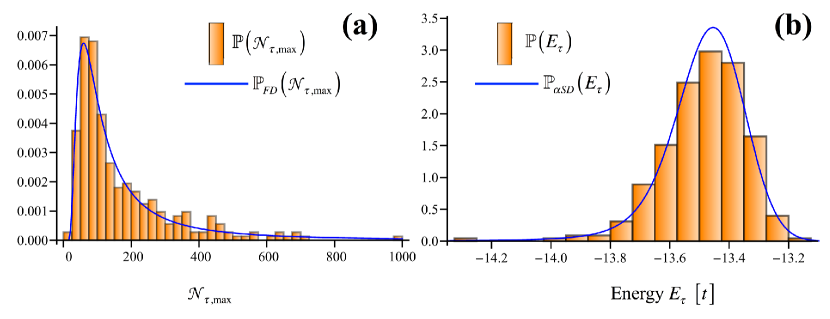
Figure 1: (Color online) Emergence of infinite-variance problems in the QMC scheme (3, 50bb) when only real stochastic wavefunctions are generated. We consider the Hubbard model (50ds) on a $4\times 4$ half-filled cluster in the repulsive regime $U=4t$ with HF walkers. The single-particle states remain real during their Brownian motion as long as the interaction term on a site ${\bf r}$ is cast into the form $2\hat{n}_{{\bf r}\uparrow}\hat{n}_{{\bf r}\downarrow}=\hat{n}_{{\bf r}\uparrow}+\hat{n}_{{\bf r}\downarrow}-\left(\hat{n}_{{\bf r}\uparrow}-\hat{n}_{{\bf r}\downarrow}\right)^{2}$. 300 independent populations, with the number of walkers fixed to $N_{w}=100$, are obtained through a semi-implicit Euler algorithm and an adaptive step control technique to solve the stochastic differential equations (3). The sampling according to the weight $\Pi_{\tau}$ is performed with a reconfiguration scheme detailed in [54]. For each population, the averaged energy $E_{\tau}=\mathbb{E}_{\Pi}\bigl{[}\langle\hat{H}\rangle_{\Psi_{T},\Phi_{\tau}}\bigr{]}$ and the norm $\mathcal{N}_{\tau}=\bigl{|}\bigl{|}{|\tilde{W}_{\tau}\rangle}\bigr{|}\bigr{|}=1/|{\langle\Psi_{T}|\Phi_{\tau}\rangle}|$ of generated walkers ${|\tilde{W}_{\tau}\rangle}={|\Phi_{\tau}\rangle}/{\langle\Psi_{T}|\Phi_{\tau}\rangle}$ are calculated as a function of the imaginary time $\tau$. According to the extreme-value theorem [55], a power-law tail $\mathcal{N}_{\tau}^{-1-\nu}$ for the distribution of $\mathcal{N}_{\tau}$ maps into a Fréchet law $\mathbb{P}_{FD}(\mathcal{N}_{\tau,{\rm max}})\propto\rme^{-(\mathcal{N}_{\tau,{\rm max}}/S)^{-\nu}}$ for the maximum value $\mathcal{N}_{\tau,{\rm max}}$ over a finite and sufficiently large sequence of realizations ($S$ is a scale parameter). (a) Histogram of the empirical probability distribution function $\mathbb{P}(\mathcal{N}_{\tau,{\rm max}})$ of $\mathcal{N}_{\tau,{\rm max}}$ at imaginary time $\tau=5/t$. The fit to the expected distribution $\mathbb{P}_{FD}(\mathcal{N}_{\tau,{\rm max}})$ is shown by the continuous line. The associated $p$-value of 0.675 in a Pearson $\chi^{2}$ test confirms the validity of the Fréchet law hypothesis. An exponent $\nu\simeq 3.94>2$ is thus extracted and indicates an infinite variance (50bi) of the error on the exact many-body state. (b) Histogram of the empirical probability distribution function $\mathbb{P}(E_{\tau})$ of the energy at imaginary time $\tau=5/t$ . The results are not normally distributed ($p$-value $\simeq 0.04$), but rather follows the asymmetric Lévy stable distribution $\mathbb{P}_{\alpha SD}(E_{\tau})$ of index $\alpha\simeq 1.776$ ($p$-value $\simeq 0.576$). Such behavior agrees with the generalized central-limit theorem for the sum of independent random variables of infinite variance. Consequently, the standard Monte-Carlo estimate $\bar{E}_{\tau}=-13.483(8)t$, for the energy $E_{\tau}$ averaged over all populations, is meaningless. Without the knowledge of an infinite-variance problem, a systematic error compared to the exact ground-state energy $E_{G}=-13.62t$ is highlighted.

To conclude, it should be noted that infinite-variance problem is not specific to the dynamics (3) considered here. The standard auxiliary-field approach (30), which explores Slater determinants and differs by the absence of local estimators $\langle\hat{O}_{s}\rangle_{\Psi_{T},\Phi}$ in the determinist evolution, generally suffers from a similar pathology when importance sampling is included and is exempt of sign problems [56].

5 Estimates of observables

5.1 General considerations

As an illustrative example, consider the determination of the energy $E_{G}$ of the ground state ${|\Psi_{G}\rangle}$. As part of an exact propagation (29) in imaginary time, we immediately obtain

$$E_{G}=\lim_{\tau\to\infty}\frac{\Re{{\langle\Psi_{T}|\hat{H}\exp\bigl{(}-\tau\hat{H}\bigr{)}|\Phi_{0}\rangle}}}{\Re{{\langle\Psi_{T}|\exp\bigl{(}-\tau\hat{H}\bigr{)}|\Phi_{0}\rangle}}},$$ (50bn)

provided the initial state ${|\Phi_{0}\rangle}$ and the trial state ${|\Psi_{T}\rangle}$ are not orthogonal to ${|\Psi_{G}\rangle}$. With the stochastic interpretation (32) of the dynamics where the walkers are generated according to the importance of their overlap with ${|\Psi_{T}\rangle}$,

$$E_{G}=\lim_{\tau\to\infty}\frac{\mathbb{E}\left[\Re{\left(\Pi_{\tau}\langle\hat{H}\rangle_{\Psi_{T},\Phi_{\tau}}\right)}\right]}{\mathbb{E}\Bigl{[}\Re{\left(\Pi_{\tau}\right)}\Bigr{]}}$$ (50bo)

follows. In practice, only one approached state ${|\tilde{\Psi}_{G}\rangle}$ is however accessible through the introduction of real positive biased weights $\tilde{\Pi}$ in place of the multiplicative factors $\Pi$, and the associated energy $\tilde{E}_{G}$ will be evaluated according to

$$\tilde{E}_{G}=\lim_{\tau\to\infty}\frac{\mathbb{E}\left[\tilde{\Pi}_{\tau}\Re{\left(\langle\hat{H}\rangle_{\Psi_{T},\Phi_{\tau}}\right)}\right]}{\mathbb{E}\left[\tilde{\Pi}_{\tau}\right]}=\lim_{\tau\to\infty}\mathbb{E}_{\tilde{\Pi}}\left[\Re{\left(\langle\hat{H}\rangle_{\Psi_{T},\Phi_{\tau}}\right)}\right]\,.$$ (50bp)

The elimination at all times of the walkers close to orthogonality with the trial state guarantees a finite variance for this energy and thus ensures the validity of its reconstruction by the Monte-Carlo techniques. Indeed,

$$\mbox{Var}_{\tilde{\Pi}}\Bigl{[}\Re{\Bigl{(}\langle\hat{H}\rangle_{\Psi_{T},\Phi_{\tau}}\Bigr{)}}\Bigr{]}\!=\!\mathbb{E}_{\tilde{\Pi}}\left[\!\left\{\tilde{E}_{G}-\Re{\left(\langle\hat{H}\rangle_{\Psi_{T},\Phi_{\tau}}\right)}\right\}^{2}\!\right]\!=\!\mathbb{E}_{\tilde{\Pi}}\left[\left\{\Re{\left(\langle\hat{H}\rangle_{\Psi_{T},\Phi_{\tau}}\right)}\right\}^{2}\right]-\tilde{E}_{G}^{2},$$ (50bq)

with $\bigl{(}\Re{\langle\hat{H}\rangle_{\Psi_{T},\Phi_{\tau}}}\bigr{)}^{2}\leq\bigl{|}\langle\hat{H}\rangle_{\Psi_{T},\Phi_{\tau}}\bigr{|}^{2}\leq{\langle\Psi_{T}|\hat{H}^{2}|\Psi_{T}\rangle}{\langle\tilde{W}_{\tau}|\tilde{W}_{\tau}\rangle}$ as a consequence of the Schwartz inequality, and therefore

$$\mbox{Var}_{\tilde{\Pi}}\left[\Re{\left(\langle\hat{H}\rangle_{\Psi_{T},\Phi_{\tau}}\right)}\right]\leq{\langle\Psi_{T}|\hat{H}^{2}|\Psi_{T}\rangle}\mbox{Var}_{\tilde{\Pi}}\bigl{[}{|\tilde{W}_{\tau}\rangle}\bigr{]}-\tilde{E}_{G}^{2}<\infty\,.$$ (50br)

These considerations extend to any observable $\hat{A}$ commuting with the Hamiltonian. In the opposite case, the analogous estimator for the energy (50bp) (obtained by replacing $\hat{H}$ by $\hat{A}$) is commonly called mixed estimator $\tilde{A}_{G}^{({\rm mix})}$ of the observable. It can only offer an approximation to the true averaged value $\tilde{A}_{G}={\langle\tilde{\Psi}_{G}|\hat{A}|\tilde{\Psi}_{G}\rangle}$ in the biased ground state through the following relation, valid only to first order in the difference

$$\tilde{A}_{G}\approx 2\tilde{A}_{G}^{({\rm mix})}-{\langle\Psi_{T}|\hat{A}|\Psi_{T}\rangle}\,.$$ (50bs)

Direct simulation of $\tilde{A}_{G}$ is however possible through the “back-propagation” technique introduced in references [57, 58]. Its principle is based again on the results established in section 3, which we will write here in terms of the infinitesimal “left” propagation of a dyad $\hat{\sigma}=\Pi{|\Phi\rangle}\langle\Psi_{T}|/{\langle\Psi_{T}|\Phi\rangle}$ built from a HFB vacuum and the trial state

$$\exp\bigl{(}-\rmd\tau\hat{H}\bigr{)}\hat{\sigma}=\mathbb{E}\left[\left(\Pi+\rmd\Pi\right)\frac{\exp\left(\rmd\hat{x}\right){|\Phi\rangle}\langle\Psi_{T}|}{{\langle\Psi_{T}|\exp\left(\rmd\hat{x}\right)|\Phi\rangle}}\right]\,,$$ (50bt)

where $\rmd\Pi$, $\rmd\hat{x}$ satisfy the conditions (50a-50c). One immediately verifies that an elementary modification of the bra $\langle\Psi_{T}|$ with the same operators $\exp\left(\rmd\hat{x}\right)$ also leads to a “right” propagation of $\hat{\sigma}$:

$$\mathbb{E}\left[\left(\Pi+\rmd\Pi\right)\frac{{|\Phi\rangle}\langle\Psi_{T}|\exp\left(\rmd\hat{x}\right)}{{\langle\Psi_{T}|\exp\left(\rmd\hat{x}\right)|\Phi\rangle}}\right]=\hat{\sigma}\exp\bigl{(}-\rmd\tau\hat{H}\bigr{)}\,.$$ (50bu)

The projection of the trial wavefunction ${|\Psi_{T}\rangle}$ on the ground state can therefore be achieved by reusing, however in reverse order, the stochastic transformations $\exp\left(\rmd\hat{x}\right)$ successively undergone by the initial HFB vector ${|\Phi_{0}\rangle}$ during its Brownian motion guided by ${|\Psi_{T}\rangle}$. This evolution in imaginary time of ${|\Psi_{T}\rangle}$ is precisely required to access the expectation values in the ground state. Indeed,

$$A_{G}={\langle{\Psi}_{G}|\hat{A}|{\Psi}_{G}\rangle}=\lim_{\tau_{K},\tau_{B}\to\infty}\frac{\Re{{\langle\Psi_{T}|\exp\bigl{(}-\tau_{B}\hat{H}\bigr{)}\hat{A}\,\exp\bigl{(}-\tau_{K}\hat{H}\bigr{)}|\Phi_{0}\rangle}}}{\Re{{\langle\Psi_{T}|\exp\bigl{(}-\tau_{B}\hat{H}\bigr{)}\exp\bigl{(}-\tau_{K}\hat{H}\bigr{)}|\Phi_{0}\rangle}}}\,.$$ (50bv)

The QMC reconstruction of this “true estimator” is thus simply based on a prolongation of the motion of the HFB walkers to the time $\tau_{K}+\tau_{B}$. However, the practical implementation of the method also needs to be capable to apply the exponential of the general one-body operators $\rmd\hat{x}$ on the considered trial state. Using an approximation ${|\Phi^{\prime}_{0}\rangle}$ of HFB type for ${|\Psi_{T}\rangle}$ is therefore natural. With such a choice to guide the realizations and constrain them through biased weights, we are finally able to completely characterize the approached ground state ${|\tilde{\Psi}_{G}\rangle}$ by determining the expectation values of interest $\tilde{A}_{G}$ according to

$$\tilde{A}_{G}=\lim_{\tau_{K},\tau_{B}\to\infty}\frac{\mathbb{E}\Bigl{[}\tilde{\Pi}_{\tau_{K}+\tau_{B}}\Re{\langle\hat{A}\rangle_{\Phi^{\prime}_{\tau_{B}},\Phi_{\tau_{K}}}}\Bigr{]}}{\mathbb{E}\Bigl{[}\tilde{\Pi}_{\tau_{K}+\tau_{B}}\Bigr{]}}\,.$$ (50bw)

Here, $\tilde{\Pi}$ and the quasiparticles $\{\hat{\gamma}_{n}\}$ of the walkers ${|\Phi\rangle}$ must be determined up to time $\tau_{K}+\tau_{B}$ via the evolution equations (3, 50bl) with the trial state ${|\Psi_{T}\rangle}={|\Phi^{\prime}_{0}\rangle}$. The HFB vacuum ${|\Phi_{\tau_{K}}\rangle}$ is defined from its intermediate solution at time $\tau_{K}$ whereas the HFB wavefunction ${|\Phi^{\prime}_{\tau_{B}}\rangle}$ results from a random walk during $\tau_{B}$, starting from ${|\Phi^{\prime}_{0}\rangle}$. Its quasiparticles are precisely obtained from the following Langevin equation in the extended one-body space

$${|\gamma^{\prime}_{n}\rangle}_{\tau+\rmd\tau}=\mathcal{O} \biggl{\{}{|\gamma^{\prime}_{n}\rangle}_{\tau} -\rmd\tau\Bigl{[}\tilde{K}^{\dagger}-\sum_{s}\omega_{s}\Bigl{(}\tilde{O}_{s}^{\dagger 2}+2\langle\hat{O}_{s}-g_{s}\rangle^{*}_{\Phi^{\prime}_{0},\Phi_{\tau_{K}+\tau_{B}-\tau}}\tilde{O}_{s}^{\dagger}\Bigr{)}\Bigr{]}{|\gamma^{\prime}_{n}\rangle}_{\tau}\biggr{.}$$ (50bx)

. $$+\sum_{s}\left(\sqrt{2\omega_{s}}\right)^{*}\rmd W_{s,\tau_{K}+\tau_{B}-\tau}\tilde{O}_{s}^{\dagger}{|\gamma^{\prime}_{n}\rangle}_{\tau}\biggr{\}},$$

where the local estimators $\langle\hat{O}_{s}\rangle_{\Phi^{\prime}_{0},\Phi_{\tau_{K}+\tau_{B}-\tau}}$ and the increments of Wiener’s processes $\rmd W_{s,\tau_{K}+\tau_{B}-\tau}$ are those used during the complementary motion of the ket ${|\Phi\rangle}$ between times $\tau_{K}$ and $\tau_{K}+\tau_{B}$.

In the end, the applicability of the extension of the “phaseless QMC” formalism to HFB states (3, 50bl, 50bp, 50bw, 50bx) is essentially based on the knowledge of the local estimators $\langle\hat{A}\rangle_{\Phi^{\prime},\Phi}$ of observables between two Bogoliubov vacua ${|\Phi\rangle}$, ${|\Phi^{\prime}\rangle}$. The overlaps ${\langle\Phi^{\prime}|\Phi\rangle}$ are also needed to bias the weights of the realizations so as to control the variance. We proceed to the determination of these quantities in the following paragraphs.

5.2 Extended Wick’s theorem

Wick’s theorem plays a key role in theoretical treatments of interacting fermionic systems using Slater determinants or HFB wavefunctions. It allows one to express the expectation value of any operator in a vacuum of particles or quasiparticles in terms of the normal and abnormal elementary contractions [59, 32]. We show in this section that the result actually remains valid for local estimators of operators between two non-orthogonal HF or HFB factorized states. We also prove that the functional of binary contractions corresponds to the expansion of a Pfaffian, which greatly facilitates the numerical evaluation for operators with more than two bodies.

With two Slater determinants, this extension of Wick’s theorem to matrix elements is at the heart of auxiliary fields QMC approaches as well as “phaseless QMC” simulations. Its well known proof is based on the same principle as the one usually presented for the expectation values [60, 32]. The hybrid case of a matrix element between a HF state and a HFB wavefunction has never been considered in a general way to our knowledge, even if some partial results have been reported [61]. Yet, it is required, for example, in the previous QMC scheme applied to HF walkers guided with a trial HFB wavefunction to absorb at least approximately the pairing correlations. Here we propose a general demonstration of Wick’s theorem for the local estimators, valid regardless of the HF or HFB nature of each of the two vacua. It is inspired by the work of Balian & Brézin about non-unitary Bogoliubov transformations [62], as well as Gaudin’s work about Wick’s theorem at finite temperature for a fermionic system without interaction [63].

Let ${|\Phi\rangle}$ and ${|\Phi^{\prime}\rangle}$ be two non-orthogonal states, each being a Slater determinant or a Bogoliubov vacuum. Our aim is to determine the matrix element between these two wavefunctions, of a product of operators which factors are arbitrary linear combinations of fermionic creation $\hat{c}^{\dagger}_{{i}}$ and annihilation $\hat{c}^{\phantom{\dagger}}_{{i}}$ operators. In other words, it is to express:

$${\langle\Phi^{\prime}|\hat{Q}_{1}\ldots\hat{Q}_{M}|\Phi\rangle}={\langle\Phi^{\prime}|\Phi\rangle}\mbox{Tr}\left[\hat{Q}_{1}\ldots\hat{Q}_{M}{|\Phi\rangle}\langle\tilde{\Phi}^{\prime}|\right],$$ (50by)

with

$$\langle\tilde{\Phi}^{\prime}|=\langle\Phi^{\prime}|/{\langle\Phi^{\prime}|\Phi\rangle},\,\,\,\mbox{and}$$ (50bz)

$$\hat{Q}_{a}=\sum_{{i}}\left(\hat{c}^{\dagger}_{{i}}Y^{*}_{{i},a}+\hat{c}^{\phantom{\dagger}}_{{i}}X^{*}_{{i},a}\right),\,\,\,\forall a=1,\ldots,M.$$ (50ca)

Let us denote $\{\hat{\gamma}_{n}^{\phantom{\dagger}}\}$ and $\{\hat{\gamma}_{n}^{\prime\phantom{\dagger}}\}$ the HF or HFB quasiparticle operators (with $1\leq n\leq d$) associated to their respective vacua ${|\Phi\rangle}$ and ${|\Phi^{\prime}\rangle}$. The corresponding orthonormal bases of the one-body extended space are designated by $\{{|\gamma_{n}\rangle},{|\bar{\gamma}_{n}\rangle}\}$ and $\{{|\gamma^{\prime}_{n}\rangle},{|\bar{\gamma}_{n}^{\prime}\rangle}\}$. Using the expansions (27, 28), the $d\times d$ matrices defined by the overlaps $\mathbb{F}_{mn}={\langle\gamma^{\prime}_{m}|\gamma_{n}\rangle}$ and $\mathbb{G}_{mn}={\langle\gamma^{\prime}_{m}|\bar{\gamma}_{n}\rangle}$ allow to relate the two families of quasiparticle through

$$\hat{\gamma}^{\prime}_{m} =\sum_{\varpi{i}}\hat{c}_{\varpi{i}}^{\dagger}{\langle\varpi{i}|\gamma^{\prime}_{m}\rangle}=\sum_{\varpi{i}}\sum_{n=1}^{d}\left(\hat{\gamma}_{n}{\langle\gamma_{n}|\varpi{i}\rangle}+\hat{\gamma}_{n}^{\dagger}{\langle\bar{\gamma}_{n}|\varpi{i}\rangle}\right){\langle\varpi{i}|\gamma^{\prime}_{m}\rangle}$$ (50cb)

$$=\sum_{n=1}^{d}\left(\mathbb{F}_{mn}^{*}\hat{\gamma}_{n}+\mathbb{G}_{mn}^{*}\hat{\gamma}_{n}^{\dagger}\right).$$

Let us note that equation (50cb) can also be obtained directly by expanding ${|\gamma^{\prime}_{m}\rangle}$ in the basis $\{{|\gamma_{n}\rangle},{|\bar{\gamma}_{n}\rangle}\}$ and using the linearity of the operators $\hat{\gamma}^{\prime\phantom{\dagger}}_{m}$, $\hat{\gamma}_{n}^{\phantom{\dagger}}$, and $\hat{\gamma}_{n}^{\dagger}$ in terms of the states ${|\gamma^{\prime}_{m}\rangle}$, ${|\gamma_{n}\rangle}$, and ${|\bar{\gamma}_{n}\rangle}$, respectively. Thus, the matrices $\mathbb{F}^{T}$ and $\mathbb{G}^{T}$ are analogous to the matrices $U$ and $V$ of the Bogoliubov transformation (6) that define ${|\Phi^{\prime}\rangle}$ when the vacuum of the original fermionic operators $\{\hat{c}_{{i}}^{\phantom{\dagger}}\}$ is replaced by the vacuum ${|\Phi\rangle}$, the one of the quasiparticles $\{\hat{\gamma}_{n}^{\phantom{\dagger}}\}$.

We show now that the matrix $\mathbb{F}$ is necessarily invertible as a result of the nonorthogonality of the states ${|\Phi\rangle}$ and ${|\Phi^{\prime}\rangle}$. In the case of two Slater determinants, $\mathbb{F}$ is reduced to a block-diagonal matrix: One of them, $f$, of size $N\times N$, contains the scalar products between the occupied one-body states in both wavefunctions, and the other one, $\bar{f}$, of size $(d-N)\times(d-N)$, entails the overlaps between empty one-body states. Besides, ${\langle\Phi^{\prime}|\Phi\rangle}$ is easily obtained from the anticommutation relation $\bigl{[}\hat{c}^{\phantom{\dagger}}_{\phi^{\prime}_{m}},\hat{c}_{\phi_{n}}^{\dagger}\bigr{]}_{+}={\langle\phi^{\prime}_{m}|\phi_{n}\rangle}\,\hat{\mathbb{I}}$, for two arbitrary individual occupied states ${|\phi^{\prime}_{m}\rangle}$ and ${|\phi_{n}\rangle}$ respectively related to the determinants ${|\Phi^{\prime}\rangle}$ and ${|\Phi\rangle}$: ${\langle\Phi^{\prime}|\Phi\rangle}=\mbox{det}f$. However, each of the two HF states can alternatively be obtained, up to a phase factor, starting from the fully filled one-body space: It suffices to annihilate the fermions occupying the one-body states ${|\bar{\phi}^{\prime}_{\mu}\rangle}$ for ${|\Phi^{\prime}\rangle}$, and ${|\bar{\phi}_{\nu}\rangle}$ for ${|\Phi\rangle}$, which should actually be empty in these determinants. Still using the anticommutator $\bigl{[}\hat{c}_{\bar{\phi}^{\prime}_{\mu}}^{\dagger},\hat{c}^{\phantom{\dagger}}_{\bar{\phi}_{\nu}}\bigr{]}_{+}={\langle\bar{\phi}^{\prime}_{\mu}|\bar{\phi}_{\nu}\rangle}\hat{\mathbb{I}}$, one now obtains ${\langle\Phi^{\prime}|\Phi\rangle}=\rme^{\rmi\theta}\mbox{det}\bar{f}^{*}$ where the global phase $\rme^{\rmi\theta}$ is determined from the components $\left\{\phi^{\prime}_{{i},n}\right\}$ and $\left\{\phi_{{i},n}\right\}$. One ends with

$$|{\langle\Phi^{\prime}|\Phi\rangle}|^{2}=|\mbox{det}\mathbb{F}|.$$ (50cc)

Equation (50cc) remains actually valid with two Bogoliubov vacua [64] or in the hybrid case of a HF wavefunction and a HFB state. Without loss of generality and to simplify the discussion, we will temporarily assume ${|\Phi^{\prime}\rangle}$ to be a coherent pair state. We can then repeat the reasoning of section 2 to write the state ${|\Phi^{\prime}\rangle}$ in a BCS-type form, namely ${|\Phi^{\prime}\rangle}=\rme^{\rmi\theta}\prod_{\alpha=1}^{d/2}\bigl{(}f_{\alpha}+g_{\alpha}\hat{\Gamma}_{\alpha}^{\dagger}\hat{\Gamma}_{\tilde{\alpha}}^{\dagger}\bigr{)}{|\Phi\rangle}$, using the Bloch-Messiah-Zumino decomposition (14) of the matrices $\mathbb{F}^{T}$ and $\mathbb{G}^{T}$, coming from the Bogoliubov transformation (50cb). Here, the operators $\hat{\Gamma}_{\alpha}^{\dagger}$ and $\hat{\Gamma}_{\tilde{\alpha}}^{\dagger}$ are linear combinations of the quasiparticles $\hat{\gamma}_{n}^{\dagger}$ (which play the role of creation operators $\hat{c}_{{i}}^{\dagger}$ in the usual case of a Bogoliubov transformation applied to a fermion vacuum); $\rme^{\rmi\theta}$ is again a phase factor and the positive real numbers $f_{\alpha}$, $g_{\alpha}$ define the canonical form of matrices $\mathbb{F}^{T}$, $\mathbb{G}^{T}$. Hence, $|{\langle\Phi^{\prime}|\Phi\rangle}|=\prod_{\alpha=1}^{d/2}f_{\alpha}$, and Onishi’s equation (50cc) is recovered, since $|\mbox{det}\mathbb{F}|=\prod_{\alpha=1}^{d/2}f_{\alpha}^{2}$ due to the Bloch-Messiah-Zumino factorization of the matrix $\mathbb{F}^{T}$. Finally, the non orthogonality of ${|\Phi\rangle}$ and ${|\Phi^{\prime}\rangle}$ guarantees the matrix $\mathbb{F}$ to be invertible, irrespective of whether they are of HF or HFB type.

Let us now introduce a non-unitary transformation of the Fock space

$$\hat{\mathcal{T}}=\exp\left(\sum_{m=1}^{d}\sum_{n=m+1}^{d}\left(\mathbb{F}^{-1}\mathbb{G}\right)_{mn}\hat{\gamma}_{m}\hat{\gamma}_{n}\right)\,.$$ (50cd)

We first show that the matrix $\mathbb{F}^{-1}\mathbb{G}$ is antisymmetric. This follows both from the fermionic algebra of the sets of quasiparticles $\left\{\hat{\gamma}_{n}\right\}$ and $\left\{\hat{\gamma}^{\prime}_{n}\right\}$ as well as from the linearity of equation (50cb). Using $\left[\hat{\gamma}^{\prime\dagger}_{m},\hat{\gamma}^{\prime\dagger}_{n}\right]_{+}=\left(\mathbb{F}\mathbb{G}^{T}+\mathbb{G}\mathbb{F}^{T}\right)_{mn}\hat{\mathbb{I}}=0$ yields $\mathbb{F}^{-1}\mathbb{G}=-\mathbb{G}^{T}\left(\mathbb{F}^{T}\right)^{-1}=-\left(\mathbb{F}^{-1}\mathbb{G}\right){}^{T}$. In addition, $\hat{\mathcal{T}}$ leaves invariant the annihilation operators of the quasiparticle in the state ${|\Phi\rangle}$, and the creation operators are transformed into linear combinations of their counterparts entering in the second wavefunction ${|\Phi^{\prime}\rangle}$. We will note $\hat{\tilde{\gamma}}_{m}{\phantom{\gamma}{}^{\prime\dagger}}$ these combinations

$$\hat{\mathcal{T}}^{-1}\hat{\gamma}_{m}\hat{\mathcal{T}} =\hat{\gamma}_{m},$$

$$\hat{\mathcal{T}}^{-1}\hat{\gamma}_{m}^{\dagger}\hat{\mathcal{T}} =\hat{\tilde{\gamma}}_{m}{\phantom{\gamma}{}^{\prime\dagger}}=\hat{\gamma}_{m}^{\dagger}-\frac{1}{2}\sum_{n,n^{\prime}=1}^{d}\left(\mathbb{F}^{-1}\mathbb{G}\right)_{nn^{\prime}}\left[\hat{\gamma}_{n}\hat{\gamma}_{n^{\prime}},\hat{\gamma}_{m}^{\dagger}\right]$$ (50ce)

$$=\hat{\gamma}_{m}^{\dagger}+\sum_{n=1}^{d}\left(\mathbb{F}^{-1}\mathbb{G}\right)_{mn}\hat{\gamma}_{n}=\sum_{n=1}^{d}\left(\mathbb{F}^{-1}\right)_{mn}\hat{\gamma}_{n}^{\prime\dagger}\,.$$

It is important to note that the so defined operators meet by construction the canonical anticommutation relations although they are not connected by the hermitian conjugation:

$$\bigl{[}\hat{\gamma}_{m},\hat{\tilde{\gamma}}_{n}{\phantom{\gamma}{}^{\prime\dagger}}\bigr{]}_{+}=\hat{\mathcal{T}}^{-1}\left[\hat{\gamma}_{m},\hat{\gamma}_{n}^{\dagger}\right]_{+}\hat{\mathcal{T}}=\delta_{m,n}\hat{\mathbb{I}}\,.$$ (50cf)

The transformation $\hat{\mathcal{T}}$ also induces a non-trivial resolution of the identity in the Fock space. Consider the orthonormal basis formed by the states ${|n_{1}\ldots n_{d}\rangle}$ of either the HF or the HFB vacuum ${|\Phi\rangle}$ by creating one or more of its quasiparticle

$${|n_{1}\ldots n_{d}\rangle}=\left(\hat{\gamma}_{1}^{\dagger}\right)^{n_{1}}\ldots\left(\hat{\gamma}_{d}^{\dagger}\right)^{n_{d}}{|\Phi\rangle},$$ (50cg)

with $n_{l}=0$ or $1$ ($l=1,\ldots,d$). Applying the inverse transformation $\hat{\mathcal{T}}^{-1}$ on these vectors, the obtained kets ${|n_{1}\ldots n_{d}\rangle}_{R}$ are no longer orthonormal and now correspond to the creation of quasiparticles $\hat{\tilde{\gamma}}_{m}{\phantom{\gamma}{}^{\prime\dagger}}$ on the state ${|\Phi\rangle}$:

$${|n_{1}\ldots n_{d}\rangle}_{R} =\hat{\mathcal{T}}^{-1}{|n_{1}\ldots n_{d}\rangle}=\left(\hat{\mathcal{T}}^{-1}\hat{\gamma}_{1}^{\dagger}\hat{\mathcal{T}}\right)^{n_{1}}\ldots\left(\hat{\mathcal{T}}^{-1}\hat{\gamma}_{d}^{\dagger}\hat{\mathcal{T}}\right)^{n_{d}}{|\Phi\rangle}$$ (50ch)

$$=\left(\hat{\tilde{\gamma}}_{1}{\phantom{\gamma}{}^{\prime\dagger}}\right)^{n_{1}}\ldots\left(\hat{\tilde{\gamma}}_{d}{\phantom{\gamma}{}^{\prime\dagger}}\right)^{n_{d}}{|\Phi\rangle}\,.$$

Here we used the invariance under $\hat{\mathcal{T}}$ or $\hat{\mathcal{T}}^{-1}$ of the vacuum ${|\Phi\rangle}$ for the operators $\hat{\gamma}_{n}$. The states (50ch) are also right eigenvectors of the non-hermitian operators $\hat{\tilde{\gamma}}_{l}{\phantom{\gamma}{}^{\prime\dagger}}\hat{\gamma}_{l}$ resulting from the transformation of the quasiparticle numbers $\hat{n}_{l}^{\phantom{\dagger}}=\hat{\gamma}_{l}^{\dagger}\hat{\gamma}_{l}^{\phantom{\dagger}}$ associated to ${|\Phi\rangle}$,

$$\hat{\tilde{\gamma}}_{l}{\phantom{\gamma}{}^{\prime\dagger}}\hat{\gamma}_{l}{|n_{1}\ldots n_{d}\rangle}_{R}=\hat{\mathcal{T}}^{-1}\hat{\gamma}_{l}^{\dagger}\hat{\mathcal{T}}\hat{\mathcal{T}}^{-1}\hat{\gamma}_{l}^{\phantom{\dagger}}\hat{\mathcal{T}}\hat{\mathcal{T}}^{-1}{|n_{1}\ldots n_{d}\rangle}=n_{l}{|n_{1}\ldots n_{d}\rangle}_{R}\,.$$ (50ci)

The adjoint basis, formed by the left eigenvectors ${\phantom{{|\rangle}}}_{L}\langle n_{1}\ldots n_{d}|$, is immediately found according to the same developments, except that the dual vectors of the occupation number representation (50cg) are transformed under $\hat{\mathcal{T}}$

$${\phantom{{|\rangle}}}_{L}\langle n_{1} \ldots n_{d}|=\langle n_{1}\ldots n_{d}|\hat{\mathcal{T}}=\langle\Phi|\hat{\mathcal{T}}\left(\hat{\mathcal{T}}^{-1}\hat{\gamma}_{d}^{\phantom{\dagger}}\hat{\mathcal{T}}\right)^{n_{d}}\ldots\left(\hat{\mathcal{T}}^{-1}\hat{\gamma}_{1}^{\phantom{\dagger}}\hat{\mathcal{T}}\right)^{n_{1}}$$ (50cj)

$$\,\,\,\,\,\,\,\,=\langle\tilde{\Phi}^{\prime}|\left(\hat{\gamma}_{d}^{\phantom{\dagger}}\right)^{n_{d}}\ldots\left(\hat{\gamma}_{1}^{\phantom{\dagger}}\right)^{n_{1}},$$

$${\phantom{{|\rangle}}}_{L}\langle n_{1} \ldots n_{d}|\hat{\tilde{\gamma}}_{l}{\phantom{\gamma}{}^{\prime\dagger}}\hat{\gamma}_{l}^{\phantom{\dagger}}=\langle n_{1}\ldots n_{d}|\hat{\mathcal{T}}\hat{\mathcal{T}}^{-1}\hat{n}_{l}^{\phantom{\dagger}}\hat{\mathcal{T}}={\phantom{{|\rangle}}}_{L}\langle n_{1}\ldots n_{d}|n_{l}\,.$$ (50ck)

These are therefore quasiparticles $\hat{\gamma}_{m}^{\dagger}$ which are created on the second vacuum ${|\tilde{\Phi}^{\prime}\rangle}$. To achieve such a result, $\hat{\mathcal{T}}$ should however connect the two considered coherent HF or HFB states : $\langle\Phi|\hat{\mathcal{T}}=\langle\tilde{\Phi}^{\prime}|$. The proof simply consists in noticing that $\langle\tilde{\Phi}^{\prime}|\hat{\mathcal{T}}^{-1}\hat{n}_{l}=\langle\tilde{\Phi}^{\prime}|\hat{\tilde{\gamma}}_{l}{\phantom{\gamma}{}^{\prime\dagger}}\hat{\gamma}_{l}^{\phantom{\dagger}}\hat{\mathcal{T}}^{-1}=0$ since $\hat{\tilde{\gamma}}_{l}{\phantom{\gamma}{}^{\prime\dagger}}$ (see equation (5.2)) is indeed a linear combination of the operators $\hat{\gamma}^{\prime\dagger}_{m}$, with $\langle\tilde{\Phi}^{\prime}|=\langle\Phi^{\prime}|/{\langle\Phi^{\prime}|\Phi\rangle}$ being their associated vacuum. As a result, the vectors $\langle\tilde{\Phi}^{\prime}|\hat{\mathcal{T}}^{-1}$ and $\langle\Phi|$ are necessarily collinear, as they both correspond to the configuration where all occupation numbers $\{n_{l}\}$ are zero. Since ${\langle\tilde{\Phi}^{\prime}|\hat{\mathcal{T}}^{-1}|\Phi\rangle}={\langle\tilde{\Phi}^{\prime}|\Phi\rangle}=1$, one thus obtains $\langle\tilde{\Phi}^{\prime}|\hat{\mathcal{T}}^{-1}=\langle\Phi|$. This result identifies to Thouless’ theorem in its most general form [65, 33]. It therefore remains valid irrespective of the HF or HFB nature of the two non-orthogonal involved vacua. Finally, we can summarize the previous results through the closure relation and the bi-orthogonality relation satisfied by the vectors (50ch) and (50cj) stemming from the Thouless transformation of the occupation-number representation

$$\sum_{\{n_{1}\ldots n_{d}\}}{{|n_{1}\ldots n_{d}\rangle}_{R}}{{\phantom{{|\rangle}}}_{L}\langle n_{1}\ldots n_{d}|}=\hat{\mathcal{T}}^{-1}\sum_{\{n_{1}\ldots n_{d}\}}{|n_{1}\ldots n_{d}\rangle}\langle n_{1}\ldots n_{d}|\hat{\mathcal{T}}=\hat{\mathbb{I}},$$ (50cl)

$${\phantom{{|\rangle}}}_{L}{\langle n_{1}\ldots n_{d}|n_{1}^{\prime}\ldots n_{d}^{\prime}\rangle}_{R}={\langle n_{1}\ldots n_{d}|\hat{\mathcal{T}}\hat{\mathcal{T}}^{-1}|n_{1}^{\prime}\ldots n_{d}^{\prime}\rangle}=\delta_{n_{1},n_{1}^{\prime}}\ldots\delta_{n_{d},n_{d}^{\prime}}\,.$$ (50cm)

Therefore, the dyad ${|\Phi\rangle}\langle\tilde{\Phi}^{\prime}|$, necessary to estimate the matrix elements (50by), can be easily extracted by eliminating all configurations with at least one quasiparticle excitation. Thanks to the previous algebraic developments, such a goal is achieved via a Gaussian non-hermitian operator

$$\hat{\mathcal{D}}=\frac{1}{\mathcal{Z}}\exp{\left(-\sum_{l=1}^{d}\vartheta_{l}\hat{\tilde{\gamma}}_{l}{\phantom{\gamma}{}^{\prime\dagger}}\hat{\gamma}_{l}^{\phantom{\dagger}}\right)},$$ (50cn)

in which the real numbers $\{\vartheta_{l}\}$ are arbitrary and $\mathcal{Z}$ ensures normalization. Physically, $\hat{\mathcal{D}}$ simply results from the Thouless transformation of the density operator describing (in the grand-canonical ensemble) the equilibrium state of an ideal quasiparticle gas $\{\hat{\gamma}_{l}\}$. In this interpretation, the parameters $\vartheta_{l}$ are therefore linked to the individual energies $\epsilon_{l}$ of these quasiparticles, to the temperature $\beta^{-1}$, and to the chemical potential $\mu$ according to $\vartheta_{l}=\beta(\epsilon_{l}-\mu)$. Besides, the Gaussian operator $\hat{\mathcal{D}}$ is diagonal in the representation (50cl) of the right and left eigenvectors of the operators $\{\hat{\tilde{\gamma}}_{l}{\phantom{\gamma}{}^{\prime\dagger}}\hat{\gamma}_{l}^{\phantom{\dagger}}\}$

$$\hat{\mathcal{D}}=\sum_{\{n_{1}\ldots n_{d}\}}{|n_{1}\ldots n_{d}\rangle}_{R}\frac{\rme^{-\vartheta_{1}n_{1}}}{1+\rme^{-\vartheta_{1}}}\ldots\frac{\rme^{-\vartheta_{d}n_{d}}}{1+\rme^{-\vartheta_{d}}}{\phantom{{|\rangle}}}_{L}\langle n_{1}\ldots n_{d}|\,.$$ (50co)

In the limit $\vartheta_{1}\to\infty,\ldots,\vartheta_{d}\to\infty$ (corresponding to zero temperature and a chemical potential $\mu<\min_{l}(\epsilon_{l})$ for the underlying perfect gas), only the configuration $n_{1}=0,\ldots,n_{d}=0$ remains and $\hat{\mathcal{D}}$ therefore reduces to the dyad ${|0\ldots 0\rangle}_{R}{\phantom{{|\rangle}}}_{L}\langle 0\ldots 0|={|\Phi\rangle}\langle\tilde{\Phi}^{\prime}|$. Eventually, we can thus bring any matrix element between two non-orthogonal states, each of HF or HFB type, to an expectation value in the Gaussian ansatz (50cn)

$${\langle\Phi^{\prime}|\hat{Q}_{1}\ldots\hat{Q}_{M}|\Phi\rangle}={\langle\Phi^{\prime}|\Phi\rangle}\lim_{\{\vartheta_{l}\to\infty\}}\langle\hat{Q}_{1}\ldots\hat{Q}_{M}\rangle_{\hat{\mathcal{D}}}\,,$$ (50cp)

where $\langle\ldots\rangle_{\hat{\mathcal{D}}}=\mbox{Tr}(\ldots\hat{\mathcal{D}})$ denotes the expectation value in a statistical mixture represented by the density operator $\hat{\mathcal{D}}$.

Let us now first focus on the simple cases where either $\hat{Q}_{1}=\hat{\tilde{\gamma}}_{l}{\phantom{\gamma}{}^{\prime\dagger}}$ or $\hat{Q}_{1}=\hat{\gamma}_{l}$. One can show that

$$\hat{\tilde{\gamma}}_{l}{\phantom{\gamma}{}^{\prime\dagger}}\hat{\mathcal{D}}=\rme^{\vartheta_{l}}\hat{\mathcal{D}}\hat{\tilde{\gamma}}_{l}{\phantom{\gamma}{}^{\prime\dagger}},\quad\hat{\gamma}_{l}\hat{\mathcal{D}}=\rme^{-\vartheta_{l}}\hat{\mathcal{D}}\hat{\gamma}_{l},$$ (50cq)

by integrating

$$\frac{\partial\bigl{(}\hat{\mathcal{D}}^{-1}\hat{Q}_{1}\hat{\mathcal{D}}\bigr{)}}{\partial\vartheta_{l}}=\hat{\mathcal{D}}^{-1}\bigl{[}\hat{\tilde{\gamma}}_{l}{\phantom{\gamma}{}^{\prime\dagger}}\hat{\gamma}_{l},\hat{Q}_{1}\bigr{]}\hat{\mathcal{D}}=\pm\bigl{(}\hat{\mathcal{D}}^{-1}\hat{Q}_{1}\hat{\mathcal{D}}\bigr{)},$$ (50cr)

that directly follows from the Gaussian form of $\hat{\mathcal{D}}$ as well as from the anticommutation relations of the operators $\hat{\tilde{\gamma}}_{l}{\phantom{\gamma}{}^{\prime\dagger}}$ and $\hat{\gamma}_{l}$. In equation (50cr), the signs $(+)$ and $(-)$ refer to $\hat{Q}_{1}=\hat{\tilde{\gamma}}_{l}{\phantom{\gamma}{}^{\prime\dagger}}$ and $\hat{Q}_{1}=\hat{\gamma}_{l}$, respectively. Under these circumstances, the cyclic invariance of the trace allows to relate the two averaged values $\langle\hat{Q}_{1}\hat{Q}_{2}\ldots\hat{Q}_{M}\rangle_{\hat{\mathcal{D}}}$ and $\langle\hat{Q}_{2}\ldots\hat{Q}_{M}\hat{Q}_{1}\rangle_{\hat{\mathcal{D}}}$ as

$$\langle\hat{Q}_{2}\ldots\hat{Q}_{M}\hat{Q}_{1}\rangle_{\hat{\mathcal{D}}} =\mbox{Tr}\left(\hat{Q}_{2}\ldots\hat{Q}_{M}\hat{Q}_{1}\hat{\mathcal{D}}\right)=\rme^{\pm\vartheta_{l}}\mbox{Tr}\left(\hat{Q}_{2}\ldots\hat{Q}_{M}\hat{\mathcal{D}}\hat{Q}_{1}\right)$$ (50cs)

$$=\rme^{\pm\vartheta_{l}}\mbox{Tr}\left(\hat{Q}_{1}\hat{Q}_{2}\ldots\hat{Q}_{M}\hat{\mathcal{D}}\right)=\rme^{\pm\vartheta_{l}}\langle\hat{Q}_{1}\hat{Q}_{2}\ldots\hat{Q}_{M}\rangle_{\hat{\mathcal{D}}}.$$

Assuming from now on that $M$ is even, the calculation of the expectation value of their product with the Gaussian density operator, possibly non-hermitian, is therefore determined through a recursive procedure defined by

$$\langle\hat{Q}_{1}\hat{Q}_{2}\ldots\hat{Q}_{M}\rangle_{\hat{\mathcal{D}}}=\sum_{b=2}^{M}(-1)^{b}\frac{\bigl{[}\hat{Q}_{1},\hat{Q}_{b}\bigr{]}_{+}}{1+\rme^{\pm\vartheta_{l}}}\langle\hat{Q}_{2}\ldots\hat{Q}_{b-1}\hat{Q}_{b+1}\ldots\hat{Q}_{M}\rangle_{\hat{\mathcal{D}}}.$$ (50ct)

When the number of factors is as small as two, we obtain the following contractions $\langle\hat{Q}_{1}\hat{Q}_{2}\rangle_{\hat{\mathcal{D}}}$:

$$\langle\hat{Q}_{1}\hat{Q}_{2}\rangle_{\hat{\mathcal{D}}}=\frac{\bigl{[}\hat{Q}_{1},\hat{Q}_{2}\bigr{]}_{+}}{1+\rme^{\pm\vartheta_{l}}}.$$ (50cu)

Let us recall that, at this stage, the operator $\hat{Q}_{1}$ is limited to either $\hat{\tilde{\gamma}}_{l}{\phantom{\gamma}{}^{\prime\dagger}}$ (+ sign) or $\hat{\gamma}_{l}$ (- sign). On the other hand, $\hat{Q}_{2}$ can be any linear combination of fermionic elementary operators. The expansion (50ct) can thus obviously be written in a linear form in the operators $\hat{Q}_{1}$ considered up to now

$$\langle\hat{Q}_{1}\hat{Q}_{2}\ldots\hat{Q}_{M}\rangle_{\hat{\mathcal{D}}}=\sum_{b=2}^{M}(-1)^{b}\langle\hat{Q}_{1}\hat{Q}_{b}\rangle_{\hat{\mathcal{D}}}\langle\hat{Q}_{2}\ldots\hat{Q}_{b-1}\hat{Q}_{b+1}\ldots\hat{Q}_{M}\rangle_{\hat{\mathcal{D}}}\,.$$ (50cv)

The generalization to any factor is immediate as long as it can be linearly expanded in terms of the quasiparticles $\{\hat{\gamma}_{l}\}$ and $\{\hat{\tilde{\gamma}}_{l}{\phantom{\gamma}{}^{\prime\dagger}}\}$. To achieve this, the kets $\{{|\gamma_{l}\rangle}\}$ and $\bigl{\{}{|\bar{\tilde{\gamma}}^{\prime}_{l}\rangle}=\sum_{m=1}^{d}\left(\mathbb{F}^{-1}\right)_{lm}{|\bar{\gamma}^{\prime}_{m}\rangle}\bigr{\}}$, on which these operators depend linearly (see equation (5.2)), must form a basis. They define two non-orthogonal subspaces and their total number is equal to $2d$, the dimension of $\mathcal{H}_{\rm ex}^{(1)}$. Hence, it just needs to be checked that they are linearly independent. If $\sum_{m=1}^{d}\left(\lambda_{m}{|\gamma_{m}\rangle}+\lambda^{\prime}_{m}{|\bar{\tilde{\gamma}}^{\prime}_{m}\rangle}\right)=0$ where $\lambda_{m}$ and $\lambda^{\prime}_{m}$ are scalar numbers, the following equations necessarily hold true

$$\sum_{m=1}^{d}\left(\lambda_{m}{\langle\gamma^{\prime}_{l}|\gamma_{m}\rangle}+\lambda^{\prime}_{m}{\langle\gamma^{\prime}_{l}|\bar{\tilde{\gamma}}^{\prime}_{m}\rangle}\right) =\sum_{m=1}^{d}\mathbb{F}_{lm}\lambda_{m}=0,$$

$$\sum_{m=1}^{d}\left(\lambda_{m}{\langle\bar{\gamma}_{l}|\gamma_{m}\rangle}+\lambda^{\prime}_{m}{\langle\bar{\gamma}_{l}|\bar{\tilde{\gamma}}^{\prime}_{m}\rangle}\right) =\sum_{m,n=1}^{d}\lambda^{\prime}_{m}\left(\mathbb{F}^{-1}\right)_{mn}{\langle\bar{\gamma}_{l}|\bar{\gamma}^{\prime}_{n}\rangle}=0\,.$$ (50cw)

The matrix $\mathbb{F}$ being invertible, the coefficients $\lambda_{m}$ are therefore zero. Returning to the amplitudes $\left\{U_{{i},l},V_{{i},l}\right\}$ and $\left\{U^{\prime}_{{i},m},V^{\prime}_{{i},m}\right\}$ of the canonical Bogoliubov transformations defining the two considered coherent states ${|\Phi\rangle}$ and ${|\Phi^{\prime}\rangle}$, respectively, it turns out that the overlaps ${\langle\bar{\gamma}^{\phantom{*}}_{l}|\bar{\gamma}^{\prime}_{n}\rangle}$ are given by the matrix transposed of $\mathbb{F}$

$${\langle\bar{\gamma}^{\phantom{*}}_{l}|\bar{\gamma}^{\prime}_{n}\rangle}={\langle U^{\phantom{*}}_{l}|U^{\prime}_{n}\rangle}+{\langle V^{\phantom{*}}_{l}|V^{\prime}_{n}\rangle}={\langle U^{\prime*}_{n}|U^{*}_{l}\rangle}+{\langle V^{\prime*}_{n}|V^{*}_{l}\rangle}={\langle\gamma^{\prime}_{n}|\gamma^{\phantom{*}}_{l}\rangle}=\mathbb{F}^{\phantom{*}}_{nl}\,.$$ (50cx)

As a result, $\sum_{m,n=1}^{d}\lambda^{\prime}_{m}\left(\mathbb{F}^{-1}\right)_{mn}{\langle\bar{\gamma}_{l}|\bar{\gamma}^{\prime}_{n}\rangle}=\lambda^{\prime}_{l}=0$ and the set $\left\{{|\gamma_{l}\rangle},{|\bar{\tilde{\gamma}}^{\prime}_{l}\rangle}\right\}$ is indeed complete. These developments show additionally that the adjoint basis consists of the bras $\bigl{\{}\langle\tilde{\gamma}^{\prime}_{l}|=\sum_{m=1}^{d}\left(\mathbb{F}^{-1}\right)_{lm}\langle\gamma^{\prime}_{m}|,\langle\bar{\gamma}_{l}|\bigr{\}}$. We may thus finally write the completeness relation in the extended one-body space

$$\sum_{l=1}^{d}\bigl{(}{|\gamma^{\phantom{*}}_{l}\rangle}\langle\tilde{\gamma}^{\prime}_{l}|+{|\bar{\tilde{\gamma}}^{\prime}_{l}\rangle}\langle\bar{\gamma}_{l}|\bigr{)}=\mathbb{I}.$$ (50cy)

By attaching the two usual vectors

$${|Q_{a}\rangle}=\left(\begin{array}[]{c}{|Y^{*}_{a}\rangle}\\ {|X^{*}_{a}\rangle}\end{array}\right)\,\,\,\mbox{and}\,\,\,{|\bar{Q}_{a}\rangle}=\left(\begin{array}[]{c}{|X_{a}\rangle}\\ {|Y_{a}\rangle}\end{array}\right),$$ (50cz)

to each operator $\hat{Q}_{a}=\sum_{{i}}\bigl{(}\hat{c}^{\dagger}_{{i}}Y^{*}_{{i},a}+\hat{c}^{\phantom{\dagger}}_{{i}}X^{*}_{{i},a}\bigr{)}$, this resolution of the identity, together with (27), induces the following expansions from the decomposition of the ket ${|Q_{a}\rangle}$ or the bra $\langle\bar{Q}_{a}|$

$$\hat{Q}^{\phantom{*}}_{a}=\sum_{l=1}^{d}\left(\hat{\gamma}^{\phantom{*}}_{l}{\langle\tilde{\gamma}^{\prime}_{l}|Q^{\phantom{*}}_{a}\rangle}+\hat{\tilde{\gamma}}_{l}{\phantom{\gamma}{}^{\prime\dagger}}{\langle\bar{\gamma}^{\phantom{*}}_{l}|{Q}^{\phantom{*}}_{a}\rangle}\right)=\sum_{l=1}^{d}\left({\langle\bar{Q}^{\phantom{*}}_{a}|\gamma^{\phantom{*}}_{l}\rangle}\hat{\tilde{\gamma}}_{l}{\phantom{\gamma}{}^{\prime\dagger}}+{\langle\bar{Q}^{\phantom{*}}_{a}|\bar{\tilde{\gamma}}_{l}\rangle}\hat{\gamma}^{\phantom{*}}_{l}\right).$$ (50da)

Therefore, any first factor $\hat{Q}_{1}$ can always be reduced to a linear combination of the quasiparticle operators $\hat{\tilde{\gamma}}_{l}{\phantom{\gamma}{}^{\prime\dagger}}$ and $\hat{\gamma}_{l}$. The relation (50cv), giving a recursive expression of the expectation value $\langle\hat{Q}_{1}\hat{Q}_{2}\ldots\hat{Q}_{M}\rangle_{\hat{\mathcal{D}}}$ in a Gaussian density operator, is therefore valid in general, and corresponds to Wick’s theorem. It only requires the knowledge of binary contractions $\langle\hat{Q}_{a}\hat{Q}_{b}\rangle_{\hat{\mathcal{D}}}$ that are, moreover, obtained by combining the expansions (50da), the previously obtained (50cu) elementary contractions $\langle\hat{\tilde{\gamma}}_{l}{\phantom{\gamma}{}^{\prime\dagger}}\hat{Q}_{b}\rangle_{\hat{\mathcal{D}}}$, $\langle\hat{\gamma}_{l}\hat{Q}_{b}\rangle_{\hat{\mathcal{D}}}$, together with the anticommutation relations (50cf) for the set $\bigl{\{}\hat{\gamma}_{l},\hat{\tilde{\gamma}}_{l}{\phantom{\gamma}{}^{\prime\dagger}}\bigr{\}}$. For example, writing $\hat{Q}_{a}$ and $\hat{Q}_{b}$ in terms of the ket ${|Q_{a}\rangle}$ and the bra $\langle\bar{Q}_{b}|$, respectively, one has

$$\langle\hat{Q}_{a}\hat{Q}_{b}\rangle_{\hat{\mathcal{D}}} =\sum_{l=1}^{d}\frac{\bigl{[}\hat{\gamma}_{l},\hat{Q}_{b}\bigr{]}_{+}}{1+\rme^{-\vartheta_{l}}}{\langle\tilde{\gamma}^{\prime}_{l}|Q_{a}\rangle}+\sum_{l=1}^{d}\frac{\bigl{[}\hat{\tilde{\gamma}}_{l}{\phantom{\gamma}{}^{\prime\dagger}},\hat{Q}_{b}\bigr{]}_{+}}{1+\rme^{\vartheta_{l}}}{\langle\bar{\gamma}_{l}|Q_{a}\rangle}$$ (50db)

$$=\sum_{l=1}^{d}\frac{{\langle\bar{Q}_{b}|\gamma_{l}\rangle}{\langle\tilde{\gamma}^{\prime}_{l}|Q_{a}\rangle}}{1+\rme^{-\vartheta_{l}}}+\sum_{l=1}^{d}\frac{{\langle\bar{Q}_{b}|\bar{\tilde{\gamma}}^{\prime}_{l}\rangle}{\langle\bar{\gamma}_{l}|Q_{a}\rangle}}{1+\rme^{\vartheta_{l}}}.$$

Equivalently, with the bra $\langle\bar{Q}_{a}|$ and the ket ${|Q_{b}\rangle}$, one gets

$$\langle\hat{Q}_{a}\hat{Q}_{b}\rangle_{\hat{\mathcal{D}}}=\sum_{l=1}^{d}\frac{{\langle\bar{Q}_{a}|\gamma_{l}\rangle}{\langle\tilde{\gamma}^{\prime}_{l}|Q_{b}\rangle}}{1+\rme^{\vartheta_{l}}}+\sum_{l=1}^{d}\frac{{\langle\bar{Q}_{a}|\bar{\tilde{\gamma}}^{\prime}_{l}\rangle}{\langle\bar{\gamma}_{l}|Q_{b}\rangle}}{1+\rme^{-\vartheta_{l}}}.$$ (50dc)

Taking into account the completeness relation (50cy) in the extended one-body space, the two expressions (50db-50dc) are identical. Besides, they have a perfectly well defined limit when $\{\vartheta_{l}\to\infty\}$, where the operator $\hat{\mathcal{D}}$ identifies to the dyad ${|\Phi\rangle}\langle\tilde{\Phi}^{\prime}|$, and gives access to the matrix elements between the two vacua (HF or HFB). Irrespective of the factors $\hat{Q}_{a}$ considered, the contractions $\langle\hat{Q}_{a}\hat{Q}_{b}\rangle_{\hat{\mathcal{D}}}$ can also be deduced from those between two elementary fermionic operators that define the generalized one-body density matrix $\mathcal{R}$

$$\mathcal{R}\!=\!\left(\begin{array}[]{cc}\rho&\kappa\\ \tilde{\kappa}&\tilde{\rho}\end{array}\right)\,\,\,\mbox{with}\,\,\,\left\{\begin{array}[]{c}\rho_{{i},{{j}}}=\langle\hat{c}^{\dagger}_{{j}}\hat{c}^{\phantom{\dagger}}_{{i}}\rangle_{\hat{\mathcal{D}}}\\[3.99994pt] \tilde{\rho}_{{i},{{j}}}=\langle\hat{c}^{\phantom{\dagger}}_{{j}}\hat{c}^{\dagger}_{{i}}\rangle_{\hat{\mathcal{D}}}\end{array}\right.\,\,\,\mbox{and}\,\,\,\left\{\begin{array}[]{c}\kappa_{{i},{{j}}}=\langle\hat{c}^{\phantom{\dagger}}_{{j}}\hat{c}^{\phantom{\dagger}}_{{i}}\rangle_{\hat{\mathcal{D}}}\\[3.99994pt] \tilde{\kappa}_{{i},{{j}}}=\langle\hat{c}^{\dagger}_{{j}}\hat{c}^{\dagger}_{{i}}\rangle_{\hat{\mathcal{D}}}\end{array}\right..$$ (50dd)

In other words, ${\langle\varpi{i}|\mathcal{R}|\varpi^{\prime}{j}\rangle}=\langle\hat{c}^{\dagger}_{\varpi^{\prime}{j}}\hat{c}^{\phantom{\dagger}}_{\varpi{i}}\rangle_{\hat{\mathcal{D}}}$ and thus

$$\langle\hat{Q}_{a}\hat{Q}_{b}\rangle_{\hat{\mathcal{D}}} =\sum_{\varpi{i}}\sum_{\varpi^{\prime}{j}}{\langle\bar{Q}_{b}|\varpi{i}\rangle}\langle\hat{c}^{\dagger}_{\varpi^{\prime}{j}}\hat{c}^{\phantom{\dagger}}_{\varpi{i}}\rangle_{\hat{\mathcal{D}}}{\langle\varpi^{\prime}{j}|Q_{a}\rangle}={\langle{\bar{Q}_{b}}|\mathcal{R}|Q_{a}\rangle}$$ (50de)

$$=\sum_{\varpi{i}}\sum_{\varpi^{\prime}{j}}{\langle\bar{Q}_{a}|\varpi{i}\rangle}\langle\hat{c}^{\phantom{\dagger}}_{\varpi{i}}\hat{c}^{\dagger}_{\varpi^{\prime}{j}}\rangle_{\hat{\mathcal{D}}}{\langle\varpi^{\prime}{j}|Q_{b}\rangle}={\langle{\bar{Q}_{a}}|\mathbb{I}-\mathcal{R}|Q_{b}\rangle}\,.$$

By virtue of the results (50db-50dc) coming from the demonstration of Wick’s theorem, $\mathcal{R}$ is thus given, in the limit of zero temperature $\{\vartheta_{l}\to\infty\}$, by

$$\mathcal{R} = \sum_{l=1}^{d}{|\gamma_{l}\rangle}\langle\tilde{\gamma}^{\prime}_{l}|=\sum_{l,m=1}^{d}{|\gamma_{l}\rangle}\left(\mathbb{F}^{-1}\right)_{lm}\langle\gamma^{\prime}_{m}|,$$

$$\mathbb{I} - \mathcal{R}=\sum_{l=1}^{d}{|\bar{\tilde{\gamma}}^{\prime}_{l}\rangle}\langle\bar{\gamma}_{l}|=\sum_{l,m=1}^{d}{|\bar{\gamma}^{\prime}_{l}\rangle}\left(\mathbb{F}^{-1}\right)_{ml}\langle\bar{\gamma}_{m}|.$$ (50df)

Eventually, $\langle\hat{Q}_{1}\hat{Q}_{2}\ldots\hat{Q}_{M}\rangle_{\hat{\mathcal{D}}}$ is a functional $\mathcal{Q}[\mathcal{R}]$ of the reduced density matrix $\mathcal{R}$ which results from the repeated application of the recursive algorithm (50cv) to estimate the expectation values of $M-2$, and then $M-4$, $\ldots$ factors. As a matter of fact, $\mathcal{Q}[\mathcal{R}]$ can be directly obtained by noting that this recurrence relation is exactly that of the development of a Pfaffian, that is to say of the square root of the determinant of an antisymmetric matrix [66, 67]. Let us introduce such a matrix $\mathcal{C}$ of dimension $M\times M$ with upper triangular entries given by the binary contractions of factors $\hat{Q}_{a}$ of the considered product $\mathcal{C}_{a,b}=\langle\hat{Q}_{a}\hat{Q}_{b}\rangle_{\hat{\mathcal{D}}}$, $a<b\in\{1,\ldots,M\}$. The Pfaffian $\mbox{Pf}(\mathcal{C})$ can then be found according to a procedure similar to that of calculating a determinant, i.e., through the expansion, for example, along the first row [67]

$$\mbox{Pf}(\mathcal{C})=\sum_{b=2}^{M}(-1)^{b}\mathcal{C}_{1,b}\mbox{Pf}(\mathcal{C}^{(1,b)}),$$ (50dg)

where $\mathcal{C}^{(1,b)}$ is the sub-matrix obtained by removing the first row and the $b$-th column. We thus immediately obtain the identity $\mathcal{Q}[\mathcal{R}]=\mbox{Pf}(\mathcal{C})$ by mathematical induction: For two factors, the definitions of the matrix $\mathcal{C}$ and of the Pfaffian indeed lead to

$$\langle\hat{Q}_{1}\hat{Q}_{2}\rangle_{\hat{\mathcal{D}}}=\mathcal{C}_{1,2}=\mbox{Pf}\left(\begin{array}[]{cc}0&\mathcal{C}_{1,2}\\ -\mathcal{C}_{1,2}&0\end{array}\right).$$ (50dh)

Assuming this result to be valid for $M-2$ factors, $\langle\hat{Q}_{2}\ldots\hat{Q}_{b-1}\hat{Q}_{b+1}\ldots\hat{Q}_{M}\rangle_{\hat{\mathcal{D}}}=\mbox{Pf}(\mathcal{C}^{(1,b)})$ follows, so that the relations (50cv, 50dg) complete the proof by leading to

$$\langle\hat{Q}_{1}\hat{Q}_{2}\ldots\hat{Q}_{M}\rangle_{\hat{\mathcal{D}}}=\mbox{Pf}(\mathcal{C}).$$ (50di)

To our knowledge, this connection between the Wick theorem and the Pfaffians has been originally highlighted by E. Lieb [68], following M. Gaudin’s work [63]. It allows, via the explicit form of the Pfaffian of a matrix in terms of its elements, to synthesize the previous results in the form

$$\langle\hat{Q}_{1}\hat{Q}_{2}\ldots\hat{Q}_{M}\rangle_{\hat{\mathcal{D}}}=\mathcal{Q}[\mathcal{R}]=\mbox{ Pf}(\mathcal{C})=\sum_{\pi}\varepsilon_{\pi}\mathcal{C}_{\pi(1),\pi(2)}\ldots\mathcal{C}_{\pi(M-1),\pi(M)},$$

$$\mathcal{C}_{ab}=\langle\hat{Q}_{a}\hat{Q}_{b}\rangle_{\hat{\mathcal{D}}}={\langle\bar{Q}_{b}|\mathcal{R}|Q_{a}\rangle}={\langle\bar{Q}_{a}|\mathbb{I}-\mathcal{R}|Q_{b}\rangle}\,.$$ (50dj)

Here, recalling that $M$ is even, the sum is performed on the $(M-1)!!$ permutations $\pi$ of the set $\{1,2,\ldots,M\}$ satisfying the constraints $\pi(2r-1)<\pi(2r+1)$ ($r=1,\ldots,M/2-1$) and $\pi(2r-1)<\pi(2r)$ ($r=1,\ldots,M/2)$, with $\varepsilon_{\pi}$ designating their signature. On top of the formal aspects, the reformulation of the Wick theorem as a Pfaffian is particularly well suited for numerical implementations for a large number of factors $\hat{Q}_{a}$, thanks to effective numerical methods to evaluate $\mbox{Pf}(\mathcal{C})$ through the determination of a tridiagonal antisymmetric form for the matrix $\mathcal{C}$ [69].

Finally, the case $\hat{Q}_{1}\hat{Q}_{2}\ldots\hat{Q}_{M}$ that we have not treated yet, where the product involves an odd number of factors, is in fact trivial and systematically leads to zero matrix elements. Indeed, the expression (50ch) of the vector ${|n_{1}\ldots n_{d}\rangle}_{R}$, as well as the canonical anticommutation relations (50cf) satisfied by the operators $\hat{\tilde{\gamma}}_{l}{\phantom{\gamma}{}^{\prime\dagger}}$ and $\hat{\gamma}_{l}$, show that these operators increase and decrease by one the occupation number $n_{l}$, respectively. An odd number of factors $\hat{Q}_{a}$ cannot therefore keep the total number of excitations $n_{1}+\ldots+n_{d}$, while the Gaussian ansatz $\hat{\mathcal{D}}$ preserves it. As a consequence,

$$\mbox{Tr}[\hat{Q}_{1}\hat{Q}_{2}\ldots\hat{Q}_{M}\hat{\mathcal{D}}]=\sum_{\{n_{1}\ldots n_{d}\}}{\phantom{{|\rangle}}}_{L}\langle n_{1}\ldots n_{d}|\hat{\mathcal{D}}\hat{Q}_{1}\ldots\hat{Q}_{M}{|n_{1}\ldots n_{d}\rangle}_{R},$$ (50dk)

vanishes necessarily.

5.3 Overlaps

Let us now show that Wick’s theorem does also give access to the overlaps ${\langle\Phi^{\prime}|\Phi\rangle}$, which are necessary to determine the matrix elements (50by) between two HF or HFB wavefunctions. With at least one HFB state among ${|\Phi\rangle}$, ${|\Phi^{\prime}\rangle}$ it should be noted that only the modulus of the overlap ${\langle\Phi^{\prime}|\Phi\rangle}$ has been determined so far through Onishi’s formula (50cc). In every approach based on a superposition of such wavefunctions, the phase of ${\langle\Phi^{\prime}|\Phi\rangle}$ obviously plays a key role and a procedure for determining it was proposed via the spectrum of the non-hermitian matrix $\mathbb{F}$ [70]. However, this method remains numerically expensive and, as a consequence, has only been concretely used for problems characterized by one-body spaces of small dimension [71]. The alternative use of Pfaffians, to directly access the overlap between two HFB states, was initiated in 2009 by Robledo through a calculation using Grassmann variables [72], which was subsequently resumed in terms of a process similar to the one that we will follow [73].

The idea rests upon Wick’s theorem, formulated in terms of a Pfaffian (5.2), after noting that all developments carried out for its demonstration remain valid if the expectations values are calculated in the vacuum of fermions ${|\;\rangle}$. Moreover, irrespective of the HF or HFB nature of each of the two wavefunctions ${|\Phi\rangle}$, ${|\Phi^{\prime}\rangle}$, they can be written as a product of factors that linearly depend on creation ($\hat{c}^{\dagger}_{{i}}$) and annihilation ($\hat{c}^{\vphantom{\dagger}}_{{i}}$) operators. Consequently, their overlap ${\langle\Phi^{\prime}|\Phi\rangle}$ identifies to the expectation value in the vacuum ${|\;\rangle}$ of such products, and it may therefore be determined thanks to Wick’s theorem. As a simple example, let us first consider the case of two Slater determinants ${|\Phi\rangle}=\hat{c}^{\dagger}_{\phi_{1}}\ldots\hat{c}^{\dagger}_{\phi_{N}}{|\;\rangle}$ and ${|\Phi^{\prime}\rangle}=\hat{c}^{\dagger}_{\phi^{\prime}_{1}}\ldots\hat{c}^{\dagger}_{\phi^{\prime}_{N}}{|\;\rangle}$, which overlap is easily obtained through a direct calculation: ${\langle\Phi^{\prime}|\Phi\rangle}=\mbox{det}(\phi^{{}^{\prime}\dagger}\phi)$. Here $\phi$ and $\phi^{\prime}$ are rectangular tables of dimensions $d\times N$ , defined by the components $\{\phi_{{i},n}\}$ and $\{\phi^{\prime}_{{i},n}\}$ of the occupied individual states of ${|\Phi\rangle}$ and ${|\Phi^{\prime}\rangle}$, respectively. Noting that $\langle\Phi^{\prime}|=(-1)^{N(N-1)/2}\langle\;|\hat{c}^{\vphantom{\dagger}}_{\phi^{\prime}_{1}}\ldots\hat{c}^{\vphantom{\dagger}}_{\phi^{\prime}_{N}}$, Wick’s theorem leads to ${\langle\Phi^{\prime}|\Phi\rangle}=(-1)^{N(N-1)/2}{\langle\;|\hat{c}^{\vphantom{\dagger}}_{\phi^{\prime}_{1}}\ldots\hat{c}^{\vphantom{\dagger}}_{\phi^{\prime}_{N}}\hat{c}^{\dagger}_{\phi_{1}}\ldots\hat{c}^{\dagger}_{\phi_{N}}|\;\rangle}=(-1)^{N(N-1)/2}\mbox{Pf}(\mathcal{C})$ where $\mathcal{C}$ is the antisymmetrized matrix of the binary contractions. Here, it is thus a $2N\times 2N$ matrix which elements are given by

$$\mathcal{C}_{{{n}}{{p}}}=\left\{\begin{array}[]{ll}{\langle\;|\hat{c}^{\vphantom{\dagger}}_{\phi^{\prime}_{{{n}}}}\hat{c}^{\vphantom{\dagger}}_{\phi^{\prime}_{{{p}}}}|\;\rangle}=0&\mbox{if }1\leq{{n}}<{{p}}\leq N\\ {\langle\;|\hat{c}^{\vphantom{\dagger}}_{\phi^{\prime}_{{{n}}}}\hat{c}^{\dagger}_{\phi_{{{p}}-N}}|\;\rangle}={\langle\phi^{\prime}_{{{n}}}|\phi_{{{p}}-N}\rangle}=\bigl{(}\phi^{{}^{\prime}\dagger}\phi\bigr{)}_{{{n}},{{p}}-N}&\mbox{if}\left\{\!\!\begin{array}[]{l}1\leq{{n}}\leq N\\ N+1\leq{{p}}\leq 2N\end{array}\right.\\ {\langle\;|\hat{c}^{\dagger}_{\phi_{{{n}}-N}}\hat{c}^{\dagger}_{\phi_{{{p}}-N}}|\;\rangle}=0&\mbox{if }N+1\leq{{n}}<{{p}}\leq 2N\end{array}\right..$$ (50dl)

In other words,

$$\mbox{Pf}(\mathcal{C})=\mbox{Pf}\left(\begin{array}[]{cc}0_{N\times N}&\phi^{{}^{\prime}\dagger}\phi\\ -\phi^{T}\phi^{{}^{\prime}*}&0_{N\times N}\end{array}\right)=(-1)^{N(N-1)/2}\mbox{det}\bigl{(}\phi^{{}^{\prime}\dagger}\phi\bigr{)}.$$ (50dm)

This follows from the properties of the Pfaffian [67] and we therefore find the expected expression for the overlap ${\langle\Phi^{\prime}|\Phi\rangle}$ between two HF vacua. The calculation is in all respects similar for two normalized HFB states, when expressed in terms of their respective quasiparticles $\{\hat{\gamma}_{n}\}$ and $\{\hat{\gamma}^{\prime}_{n}\}$ under the form of (24)

$${|\Phi\rangle}=\frac{1}{\nu_{1}\ldots\nu_{d/2}}\hat{\gamma}_{1}\ldots\hat{\gamma}_{d}{|\;\rangle},\;\;\;{|\Phi^{\prime}\rangle}=\frac{1}{\nu^{\prime}_{1}\ldots\nu^{\prime}_{d/2}}\hat{\gamma}^{\prime}_{1}\ldots\hat{\gamma}^{\prime}_{d}{|\;\rangle}\,.$$ (50dn)

We denote by $\{U_{{i},n},V_{{i},n}\}$ ($\{U^{\prime}_{{i},n},V^{\prime}_{{i},n}\}$) the amplitudes of the Bogoliubov transformation associated to ${|\Phi\rangle}$ (${|\Phi^{\prime}\rangle}$). In equation (50dn), the set of real numbers $\{v_{\alpha}\}$ ($\{v^{\prime}_{\alpha}\}$) define the Bloch-Messiah-Zumino decomposition of the matrix $V$ ($V^{\prime}$). Wick’s theorem then allows to express the expectation value ${\langle\;|\hat{\gamma}^{{}^{\prime}\dagger}_{1}\ldots\hat{\gamma}^{{}^{\prime}\dagger}_{d}\hat{\gamma}^{\vphantom{\dagger}}_{1}\ldots\hat{\gamma}^{\vphantom{\dagger}}_{d}|\;\rangle}$ of the product of all quasiparticle operators in terms of binary contractions

$$\mathcal{C}_{{{n}}{{p}}}=\left\{\begin{array}[]{ll}{\langle\;|\hat{\gamma}^{{}^{\prime}\dagger}_{{n}}\hat{\gamma}^{{}^{\prime}\dagger}_{{p}}|\;\rangle}=\bigl{(}V^{{}^{\prime}T}U^{\prime}\bigr{)}_{{{n}}{{p}}}&\mbox{if }1\leq{{n}}<{{p}}\leq d\\ {\langle\;|\hat{\gamma}^{{}^{\prime}\dagger}_{{n}}\hat{\gamma}_{{{p}}-d}|\;\rangle}=\bigl{(}V^{{}^{\prime}T}V^{*}\bigr{)}_{{{n}},{{p}}-d}&\mbox{if}\left\{\!\!\begin{array}[]{l}1\leq{{n}}\leq d\\ d+1\leq{{p}}\leq 2d\end{array}\right.\\ {\langle\;|\hat{\gamma}_{{{n}}-d}\hat{\gamma}_{{{p}}-d}|\;\rangle}=\bigl{(}U^{\dagger}V^{*}\bigr{)}_{{{n}}-d,{{p}}-d}&\mbox{if }d+1\leq{{n}}<{{p}}\leq 2d\end{array}\right.,$$ (50do)

since $(V^{{}^{\prime}T}U^{\prime})_{{{n}}{{p}}}=\sum_{{i},{j}}V^{\prime}_{{j},{{n}}}U^{\prime}_{{i},{{p}}}{\langle\;|\hat{c}^{\vphantom{\dagger}}_{{j}}\hat{c}^{\dagger}_{{i}}|\;\rangle}$, and accordingly for the other two types of matrix elements. Noting that the unitarity of Bogoliubov’s transformations implies that the matrices $V^{{}^{\prime}T}U^{\prime}$ and $U^{\dagger}V^{*}$ are antisymmetric, the overlap between two HFB states finally reads

$${\langle\Phi^{\prime}|\Phi\rangle}=\frac{(-1)^{d(d-1)/2}}{\nu^{\prime}_{1}\nu^{\vphantom{{}^{\prime}}}_{1}\ldots\nu^{\prime}_{d/2}\nu^{\vphantom{{}^{\prime}}}_{d/2}}\mbox{Pf}\left(\begin{array}[]{cc}V^{{}^{\prime}T}U^{\prime}&V^{{}^{\prime}T}V^{*}\\ -V^{\dagger}V^{\prime}&U^{\dagger}V^{*}\end{array}\right).$$ (50dp)

We refer to [73] and [72] to prove that this expression reduces to Onishi’s formula (50cc) for the square of the modulus of the scalar product between the two wavefunctions. Finally, in the hybrid case of a Bogoliubov vacuum ${|\Phi\rangle}$ (see equation (24)) and a Slater determinant ${|\Phi^{\prime}\rangle}=\hat{c}^{\dagger}_{\phi^{\prime}_{1}}\ldots\hat{c}^{\dagger}_{\phi^{\prime}_{N}}{|\;\rangle}$, one now needs to calculate ${\langle\;|\hat{c}^{\vphantom{\dagger}}_{\phi^{\prime}_{1}}\ldots\hat{c}^{\vphantom{\dagger}}_{\phi^{\prime}_{N}}\hat{\gamma}_{1}\ldots\hat{\gamma}_{d}|\;\rangle}$, i. e., the contractions

$$\mathcal{C}_{{{n}}{{p}}}=\left\{\begin{array}[]{ll}{\langle\;|\hat{c}^{\vphantom{\dagger}}_{\phi^{\prime}_{{{n}}}}\hat{c}^{\vphantom{\dagger}}_{\phi^{\prime}_{{{p}}}}|\;\rangle}=0&\mbox{if }1\leq{{n}}<{{p}}\leq N\\ {\langle\;|\hat{c}^{\vphantom{\dagger}}_{\phi^{\prime}_{{{n}}}}\hat{\gamma}^{\vphantom{\dagger}}_{{{p}}-N}|\;\rangle}=\bigl{(}\phi^{{}^{\prime}\dagger}V^{*}\bigr{)}_{{{n}},{{p}}-N}&\mbox{if}\left\{\!\!\begin{array}[]{l}1\leq{{n}}\leq N\\ N+1\leq{{p}}\leq N+d\end{array}\right.\\ {\langle\;|\hat{\gamma}^{\vphantom{\dagger}}_{{{n}}-d}\hat{\gamma}^{\vphantom{\dagger}}_{{{p}}-N}|\;\rangle}=\bigl{(}U^{\dagger}V^{*}\bigr{)}_{{{n}}-N,{{p}}-N}=0&\mbox{if }N+1\leq{{n}}<{{p}}\leq N+d,\end{array}\right.$$ (50dq)

where we used $\bigl{(}\phi^{{}^{\prime}\dagger}V^{*}\bigr{)}_{{{n}},{{p}}-N}=\sum_{{i},{j}}\phi^{{}^{\prime}*}_{{j},{{n}}}V^{*}_{{i},{{p}}-N}{\langle\;|\hat{c}^{\dagger}_{{i}}\hat{c}^{\vphantom{\dagger}}_{{j}}|\;\rangle}$. As a result, the overlap is now given by the Pfaffian of a square matrix of dimensions $N+d$

$${\langle\Phi^{\prime}|\Phi\rangle}=\frac{(-1)^{N(N-1)/2}}{\nu^{\vphantom{{}^{\prime}}}_{1}\ldots\nu^{\vphantom{{}^{\prime}}}_{d/2}}\mbox{Pf}\left(\begin{array}[]{cc}0_{N\times N}&\phi^{{}^{\prime}\dagger}V^{*}\\ -V^{\dagger}\phi^{{}^{\prime}*}&U^{\dagger}V^{*}\end{array}\right)\,.$$ (50dr)

6 Numerical illustration with the Hubbard model

Simultaneously introduced in 1963 by J. Hubbard [74], M. C. Gutzwiller [75] et J. Kanamori [76], the Hubbard model is among the simplest and the most commonly used ones in theoretical condensed-matter physics. It aims to grasp the generic properties of spin-1/2 fermions moving on a lattice by hopping between neighboring sites $<{\bf r},{\bf r^{\prime}}>$ and experiencing a local two-body interaction of strength $U$. In second-quantized form, the Hamiltonian is given by

$$\hat{H}=-t\sum_{<{\bf r},{\bf r^{\prime}}>,\sigma=\uparrow,\downarrow}\hat{c}^{\dagger}_{{\bf r}\sigma}\hat{c}^{\vphantom{dagger}}_{{\bf r^{\prime}}\sigma}+U\sum_{{\bf r}}\hat{n}^{\vphantom{dagger}}_{{\bf r}\uparrow}\hat{n}^{\vphantom{dagger}}_{{\bf r}\downarrow},$$ (50ds)

with $t$ the hopping integral; The fermionic creation, annihilation and density operators at site ${\bf r}$ with spin $\sigma\in\{\uparrow,\downarrow\}$ are $\hat{c}^{\dagger}_{{\bf r}\sigma}$, $\hat{c}^{\vphantom{dagger}}_{{\bf r}\sigma}$, and $\hat{n}^{\vphantom{dagger}}_{{\bf r}\sigma}=\hat{c}^{\dagger}_{{\bf r}\sigma}\hat{c}^{\vphantom{dagger}}_{{\bf r}\sigma}$, respectively. In the positive $U$ regime, the on-site repulsion stands for a perfectly screened Coulomb interaction and the model received a considerable renewed interest in two-dimensional (2D) geometry after Anderson’s proposal in connection to high-$T_{c}$ SC cuprates [77]. However, there is still no consensus about the adequacy of the repulsive 2D Hubbard model to capture the interplay between $d$-wave superconductivity, magnetism and inhomogeneous phases of copper oxides. In particular, constrained-path auxiliary-field QMC simulations do not give a clear answer as to the relevance, or not, of $d$-wave pair condensation that is yet obtained with variational schemes [78, 79].

As an application of the above developed “Phaseless QMC” approach, we focus here on the attractive sector, for which the stochastically explored HFB states a priori constitute an appealing approximation. Moreover, one only has to consider spin polarized systems at half-filling for the ground-state correlations to be directly related to those exhibited in the doped repulsive case [80]. This result is an immediate consequence of Shiba’s particle-hole transformation [81], given for a 2D square lattice by

$$\hat{c}^{\dagger}_{{\bf r}\uparrow}\to\hat{\underline{c}}^{\dagger}_{{\bf r}\uparrow},\;\;\;\hat{c}^{\dagger}_{{\bf r}\downarrow}\to(-1)^{x+y}\hat{\underline{c}}^{\vphantom{\dagger}}_{{\bf r}\downarrow}.$$ (50dt)

Indeed, up to an additive constant, the Hubbard Hamiltonian is recovered for the transformed fermions but with the sign of the on-site interaction changed into its opposite. Moreover, asymmetrical fillings of the two spin projections $N_{\uparrow}=\mathcal{N}(1-\delta)/2$, $N_{\downarrow}=\mathcal{N}(1+\delta)/2$ (where $\mathcal{N}$ is the number of sites and $0\leq\delta\leq 1$) become $\underline{N}_{\uparrow}=\underline{N}_{\downarrow}=\mathcal{N}(1-\delta)/2$. After transformation they thus correspond to a hole doping $\delta$. In addition, an SC homogeneous phase is linked to an antiferromagnetic order which is relevant for the repulsive model in the vicinity of the Mott insulator: $\langle\hat{c}^{\vphantom{\dagger}}_{{\bf r}\downarrow}\hat{c}^{\vphantom{\dagger}}_{{\bf r}\uparrow}\rangle\to(-1)^{x+y}\langle\hat{\underline{c}}^{\dagger}_{{\bf r}\downarrow}\hat{\underline{c}}^{\vphantom{\dagger}}_{{\bf r}\uparrow}\rangle$. Likewise, a $d$-wave spin-density wave is the counterpart of the superconductivity expected for $U>0$, $\delta>0$: $(-1)^{x+y}\langle\hat{c}^{\dagger}_{{\bf r}\downarrow}\hat{c}^{\vphantom{\dagger}}_{{\bf r}+{\bf u}_{x}\uparrow}-\hat{c}^{\dagger}_{{\bf r}\downarrow}\hat{c}^{\vphantom{\dagger}}_{{\bf r}+{\bf u}_{y}\uparrow}\rangle\to\langle\hat{\underline{c}}^{\vphantom{\dagger}}_{{\bf r}\downarrow}\hat{\underline{c}}^{\vphantom{\dagger}}_{{\bf r}+{\bf u}_{x}\uparrow}-\hat{\underline{c}}^{\vphantom{\dagger}}_{{\bf r}\downarrow}\hat{\underline{c}}^{\vphantom{\dagger}}_{{\bf r}+{\bf u}_{y}\uparrow}\rangle$. In the attractive and spin-polarized regime that we consider, these observations thus motivate the construction of a HFB approximation from a simple one-body Hamiltonian $\hat{h}_{0}$, including the two previous channels,

$$\hat{h}_{0}= - t\sum_{<{\bf r},{\bf r^{\prime}}>,\sigma=\uparrow,\downarrow}\hat{c}^{\dagger}_{{\bf r}\sigma}\hat{c}^{\vphantom{dagger}}_{{\bf r^{\prime}}\sigma}+\Delta\sum_{{\bf r}}\left(\hat{c}^{\dagger}_{{\bf r}\uparrow}\hat{c}^{\dagger}_{{\bf r}\downarrow}+\hat{c}^{\vphantom{\dagger}}_{{\bf r}\downarrow}\hat{c}^{\vphantom{\dagger}}_{{\bf r}\uparrow}\right)$$ (50du)

$$+ m_{d}\sum_{{\bf r},{\bf l}\in\{\pm{\bf u}_{x},\pm{\bf u}_{y}\}}f({\bf l})(-1)^{x+y}\left(\hat{c}^{\dagger}_{{\bf r}\uparrow}\hat{c}^{\vphantom{\dagger}}_{{\bf r}+{\bf l}\downarrow}+\hat{c}^{\dagger}_{{\bf r}\downarrow}\hat{c}^{\vphantom{\dagger}}_{{\bf r}-{\bf l}\uparrow}\right),$$

where $f(\pm{\bf u}_{x})=1$, $f(\pm{\bf u}_{y})=-1$. Here, $\Delta$ and $m_{d}$ play the role of the parameters related to the orders respectively associated to the condensation of Cooper pairs with $s$-wave symmetry and $d$-wave bond-spin antiferromagnetism. They are here a priori fixed, and no self-consistency is considered. In other words, we limit ourselves to the determination of the HFB ground state ${|\Phi_{0}\rangle}$ of (50du) under the constraint that both spin sectors are correctly populated on average. In the following, the stochastic dynamics at the heart of the “Phaseless QMC” scheme will be initiated by this vector ${|\Phi_{0}\rangle}$ and guided by a trial state ${|\Psi_{T}\rangle}$ stemming from its projection on the considered fermionic numbers $N_{\uparrow}$, $N_{\downarrow}$, i.e.

$${|\Psi_{T}\rangle}=\hat{P}_{N_{\uparrow},N_{\downarrow}}{|\Phi_{0}\rangle}.$$ (50dv)

It should be noted that the presence of the projector $\hat{P}_{N_{\uparrow},N_{\downarrow}}$ is essential to ensure a strict preservation of the total density as well as the spin polarization in the QMC simulation: With the choice (50dv) for the trial state, $\langle\hat{N}_{\uparrow}\rangle_{\Psi_{T},\Phi_{\tau}}$ and $\langle\hat{N}_{\downarrow}\rangle_{\Psi_{T},\Phi_{\tau}}$ remain unchanged irrespective of the HFB stochastic realization ${|\Phi_{\tau}\rangle}$ and independently of the imaginary time $\tau$. In practice, the restoration of the quantum numbers $(N_{\uparrow},N_{\downarrow})$ is carried out by the superposition of gauge transformations

$$\hat{P}_{N_{\uparrow},N_{\downarrow}}=\frac{1}{4\pi^{2}}\int_{0}^{2\pi}\!\!\!\int_{0}^{2\pi}\!\prod_{\sigma}d\varphi_{\sigma}\rme^{-i\varphi_{\sigma}N_{\sigma}}\rme^{\rmi\varphi_{\sigma}\hat{N}_{\sigma}}\,.$$ (50dw)

Given the developments presented in Section 3, each of them transforms the HFB wavefunction ${|\Phi_{0}\rangle}$ into another one ${|\Phi_{0}^{\prime}(\bm{\varphi})\rangle}$ where the vector $\bm{\varphi}$ gathers the two gauge angles $(\varphi_{\uparrow},\varphi_{\downarrow})$. In the extended one-body space, the states ${|\gamma_{n}\rangle}_{0}$ and ${|\gamma_{n}^{\prime}(\bm{\varphi})\rangle}_{0}$ of their respective quasiparticles are related by

$${|\gamma_{n}^{\prime}(\bm{\varphi})\rangle}_{0}=\left(\begin{array}[]{cc}\rme^{\rmi(\varphi_{\uparrow}+\varphi_{\downarrow})}\mathbb{I}_{d\times d}&0_{d\times d}\\ 0_{d\times d}&\rme^{-i(\varphi_{\uparrow}+\varphi_{\downarrow})}\mathbb{I}_{d\times d}\end{array}\right){|\gamma_{n}\rangle}_{0}\,.$$ (50dx)

Thus, the trial state ${|\Psi_{T}\rangle}$ appears as a linear combination of Bogoliubov vacua so that any local estimator $\langle\hat{A}\rangle_{\Psi_{T},\Phi_{\tau}}$ is easily evaluated through the overlaps ${\langle\Phi_{0}^{\prime}(\bm{\varphi})|\Phi_{\tau}\rangle}$ and the extended Wick theorem which gives access to ${\langle\Phi_{0}^{\prime}(\bm{\varphi})|\hat{A}|\Phi_{\tau}\rangle}/{\langle\Phi_{0}^{\prime}(\bm{\varphi})|\Phi_{\tau}\rangle}$. Finally, the implementation of the “Phaseless QMC” approach to the Hubbard model requires for the Hamiltonian (50ds) a quadratic form of general one-body operators, thus ensuring that the Bogoliubov transformation matrices are not real throughout the stochastic evolution. In this case, this step is immediate by writing

$$\hat{H}=-t\sum_{<{\bf r},{\bf r^{\prime}}>\\ \sigma=\uparrow,\downarrow}\hat{c}^{\dagger}_{{\bf r}\sigma}\hat{c}^{\vphantom{dagger}}_{{\bf r^{\prime}}\sigma}+\frac{U}{4}\sum_{{\bf r}}\Bigl{[}\bigl{(}\hat{n}^{\vphantom{dagger}}_{{\bf r}\uparrow}+\hat{n}^{\vphantom{dagger}}_{{\bf r}\downarrow}\bigr{)}^{2}-\bigl{(}\hat{n}^{\vphantom{dagger}}_{{\bf r}\uparrow}-\hat{n}^{\vphantom{dagger}}_{{\bf r}\downarrow}\bigr{)}^{2}\Bigr{]}\,.$$ (50dy)

With $U<0$, the introduction of local spin polarization $\hat{n}^{\vphantom{dagger}}_{{\bf r}\uparrow}-\hat{n}^{\vphantom{dagger}}_{{\bf r}\downarrow}$ indeed leads to purely imaginary fluctuating contributions in the Brownian motion (3) of the quasiparticles, while the on-site density $\hat{n}^{\vphantom{dagger}}_{{\bf r}\uparrow}+\hat{n}^{\vphantom{dagger}}_{{\bf r}\downarrow}$ induces a strictly real diffusive part.

\psfrag{XXXXX}{$\,\,\,\,\bm{\bar{E}_{\tau}\,[t]}$}\psfrag{YYYY}{$\,\,\,\,\bm{\tau\,[1/t]}$}\includegraphics*[width=433.62pt]{fig-energy.eps}

Figure 2: (Color online) Imaginary-time evolution of the energy $\bar{E}_{\tau}$, the average over all populations of $E_{\tau}=\mathbb{E}_{\tilde{\Pi}}\bigl{[}\Re{\bigl{(}\langle\hat{H}\rangle_{\Psi_{T},\Phi_{\tau}}\bigr{)}}\bigr{]}$, for the Hubbard Model with $U=-8t$. In panel (a), a half-filled $6\times 6$ cluster with $N_{\uparrow}=12$ and $N_{\downarrow}=24$ (using periodic boundary conditions in both directions) is considered. Panel (b) addresses the half-filled $8\times 8$ cluster with a smaller spin polarization $N_{\uparrow}=31$ and $N_{\downarrow}=33$ (using mixed periodic-antiperiodic boundary conditions, to ease the comparison with existing variational calculations in the repulsive model). In both cases the trial state follows from the constrained diagonalization of the one-body Hamiltonian $\hat{h}_{0}$ (50du) with the fixed order parameters $\Delta=0.5t$ and $m_{d}=0.1t$. The averages and error bars arise from 25 and 40 independent populations of $N_{w}=1000$ walkers in part (a) and (b), respectively. The statistical fluctuations are smaller than the size of the points when the full evolution is presented. Therefore, they are made visible in the corresponding insets.

We display in figure 2 the results obtained for the Hubbard model in the strongly attractive and spin asymmetric regime. For both studied polarizations and cluster sizes, this preliminary numerical application of our approach proves the convergence and stability of the averaged energy against a long imaginary-time propagation. The bound statistical errors at any $\tau$ give good evidence that the phase problem, as well as the sampling of regions where walkers are almost orthogonal to the trial state, are well mastered. We finally discuss the quality of the approximate ground state resulting from the use of biased weights (50bl). For this purpose we map the obtained energy onto the equivalent repulsive model. For the $6\times 6$ cluster, the estimated value at $\tau=10t$ is $\underline{\tilde{E}}_{G}=-37.29(2)t$ that compares very favorably to the virtually exact value $E_{G}=-37.41(6)t$ [82]. The latter was obtained from QMC calculations with HF walkers in the repulsive sector, starting from a constrained-path approximation that is later on released. In [82], the trial state consists of a large superposition of Slater determinants. It yields a sizeable improvement on the simple restricted-path approach, with one single HF wavefunction. Indeed, the corresponding energy is $-36.68(7)t$. Our phaseless QMC calculations with HFB walkers outperforms this standard value by nearly 2%. To our knowledge, no released constraint results for the $8\times 8$ cluster are available, and we therefore compare with variational Monte Carlo simulations. Using an extended BCS-Gutzwiller wavefunction, Eichenberger and Baeriswyl found the variational bound $E_{G}\leq-36.04t$ [83]. With $\underline{\tilde{E}}_{G}=-37.36(4)t$, our scheme yields a lower energy. These results are encouraging and need to be confirmed by a detailed examination of the physical content of the reconstructed wavefunctions through, e.g., the calculation of correlation functions. They will be the purpose of a forthcoming publication.

7 Summary and Perspectives

Summarizing, we introduced in this work a QMC theoretical framework amenable to the computation of an approximate ground state of strongly correlated superconducting fermions. It relies on HFB wavefunctions that undergo a Brownian motion in imaginary time. As compared to standard auxiliary-field QMC schemes, each stochastic path can absorb fermion pair condensation that otherwise would require a large superposition of HF realizations. The efficiency is also improved by guiding the dynamics to generate walkers according to the importance of their overlap with a trial wavefunction. A restricted-path approximation is further implemented to prevent the development of an infinite-variance problem by adequately sampling the directions almost orthogonal to the trial state. Finally, the notorious phase problem is managed through a fixed phase imposed to the overlap with the approximate ground state reached at large imaginary time. Contrary to real-space QMC methods, simulations can be performed by choosing any single-particle basis. Any physical quantity can also be estimated by applying an extension of Wick’s theorem that we have formulated in terms of Pfaffians to avoid the combinatorial complexity of standard expansions in products of binary contractions.

In condensed-matter physics, we expect our framework to help shedding new light on the microscopic mechanisms leading to the formation of unconventional Cooper pairs, such as the ones realized in the superconducting cuprates and heavy fermion materials. Besides, the phaseless QMC approach with stochastic HFB wavefunctions could unravel the degree of intertwining of order parameters arising in systems exhibiting long wave-length modes. Another field of application lies in synthetic quantum matter with ultra-cold atoms that can emulate attractive Fermi systems. In particular, the formalism is well suited to the investigation of rotating superfluid Fermi gases in the strongly interacting regime. Exotic pairing modes induced by artificial spin-orbit couplings or in multicomponent gases could be addressed too.

Bibliography

Bibliography

- [1] Kamerlingh Onnes H 1911 Proc. K. Ned. Akad. Wet. 13 1274; ibid 14 113
- [2] Matthias B T, Geballe T H, Willens R H, Corenzwit E and Hull G W 1965 Phys. Rev. 139 A1501
- [3] Drozdov A P, Eremets M I, Troyan I A, Ksenofontov V and Shylin S I 2015 Nature 525 73
- [4] Thalmeier P, Zwicknagl G, Stockert O, Sparn G and Steglich F 2005 Frontiers in Superconducting Materials (Berlin: Springer/ed. A. V. Narlikar) p 109
- [5] Jourdan M, Huth M and Adrian H 1999 Nature 398 47
- [6] Yuan H Q, Grosche F M, Deppe M, Geibel C, Sparn G and Steglich F 2003 Science 302 2104
- [7] Bruls G et al. 1994 Phys. Rev. Lett. 72 1754
- [8] Himeda A, Kato T and Ogata M 2002 Phys. Rev. Lett. 88 117001
- [9] Raczkowski M, Capello M, Poilblanc D, Frésard R and Oleś A M 2007 Phys. Rev. B 76 140505(R)
- [10] Hamidian M H et al. 2016 Nature 532 343
- [11] Fradkin E, Kivelson S A and Tranquada J M 2015 Rev. Mod. Phys. 87 457
- [12] Leprévost A, Juillet O and Frésard R 2015 New J. Phys. 17 103023
- [13] Ren Z-H et al. 2008 EPL 83 17002
- [14] Maeno Y, Rice T M and Sigrist M 2001 Phys. Today 54 42
- [15] Giamarchi T and Lhuillier C 1991 Phys. Rev. B 43 12943
- [16] Misawa T and Imada M 2014 Phys. Rev. B 90 115137
- [17] Hirsch J E 1985 Phys. Rev. B 31 4403
- [18] White S R, Scalapino D J, Sugar R L, Loh E Y, Gubernatis J E and Scalettar R T 1989 Phys. Rev. B 40 506
- [19] Meng Z Y, Lang T C, Wessel S, Assaad F F and Muramatsu A 2010 Nature (London) 464 847
- [20] Sorella S, Otsuka Y, Yunoki S 2012 Scientific Reports 2 992
- [21] Grover T 2013 Phys. Rev. Lett. 111 130402
- [22] Assaad F F, Lang T C and Toldin F P 2014 Phys. Rev. B 89 125121
- [23] Troyer M and Wiese U 2005 Phys. Rev. Lett. 94 170210
- [24] Ceperley D M and Alder B J 1980 Phys. Rev. Lett. 45 566
- [25] Reynolds P J, Ceperley D M, Alder B J and Lester Jr W A 1982 J. Chem. Phys. 77 5593
- [26] Foulkes W M C, Mitas L, Needs R J and Rajagopal G 2001 Rev. Mod. Phys. 73 33
- [27] Wu C and Zhang S-C 2005 Phys. Rev. B 71 155115
- [28] Zhang S, Carlson J and Gubernatis J E 1995 Phys. Rev. Lett. 74 3652
- [29] Zhang S 1999 Phys. Rev. Lett. 83 2777
- [30] Zhang S and Krakauer H 2003 Phys. Rev. Lett. 90 136401
- [31] Anderson J B 1975 J. Chem. Phys. 63 1499
- [32] Blaizot J -P and Ripka G 1985 Quantum Theory of Finite Systems (Cambridge: The MIT Press, MA)
- [33] Ring P and Schuck P 2003 The Nuclear Many-Body Problem (New-York/Berlin: Springer-Verlag)
- [34] Zhang W, Feng D H and Gilmore R 1990 Rev. Mod. Phys. 62 867
- [35] Bloch C and Messiah A 1962 Nucl. Phys. 39 95
- [36] Zumino B 1962 J. Math. Phys. 3 1055
- [37] Sugiyama G and Koonin S E 1986 Ann. Phys. (N.Y.) 168 1
- [38] Hirsch J E 1983 Phys. Rev. B 28 4059(R)
- [39] Carusotto I, Castin Y and Dalibard J 2001 Phys. Rev. A 63 023606
- [40] Juillet O and Chomaz Ph 2003 Phys. Rev. Lett. 88 142503
- [41] Juillet O, Gulminelli F and Chomaz Ph 2004 Phys. Rev. Lett. 92 160401
- [42] Al-Saidi W A, Zhang S, Krakauer H 2006 J. Chem. Phys. 124 224101
- [43] Wouters S, Verstichel B, Van Neck D and Kin-Lic Chan G 2014 Phys. Rev. B 90 045104
- [44] Bonnard J and Juillet O 2013 Phys. Rev. Lett. 111 012502
- [45] Bonnard J and Juillet O 201 2016 Eur. Phys. J. A 52 110
- [46] Zhang S 2013 Emergent Phenomena in Correlated Matter Modeling and Simulation (Verlag des Forschungszentrum Jülich vol 3) ed Pavarini E, Koch E, and Schollwöck U (Jülich: Forschungszentrum Jülich GmbH) pp 449-81
- [47] Lang G H, Johnson C W, Koonin S E and Ormand W E 1993 Phys. Rev. C 48 1518
- [48] Gardiner C W 1983 Handbook of Stochastic Methods (Berlin: Springer-Verlag)
- [49] Corney J F and Drummond P D 2006 Phys. Rev. B 73 125112
- [50] Bonnard J 2012 Approches Monte-Carlo Quantiques à Chemins Contraints pour le Modèle en Couches Nucléaire (PhD thesis) Université de Caen/Basse-Normandie (in French)
- [51] Corney J F and Drummond P D 2004 Phys. Rev. Lett. 93 260401
- [52] Juillet O 2007 New J. Phys. 9 163
- [53] Corboz P R, Kleine A, Assaad F F, McCulloch I P, Schollwöck U and Troyer M 2008 Phys. Rev. B 77 085108
- [54] Buonaura M C and Sorella S 1998 Phys. Rev. B 57 11446
- [55] Kotz S and Nadarajah S 2000 Extreme Value Distributions : Theory and Applications (London: Imperial College Press)
- [56] Shi H and Zhang S 2016 Phys. Rev. E 93 033303
- [57] Zhang S, Carlson J and Gubernatis J E 1997 Phys. Rev. B 55 7464
- [58] Purwanto W and Zhang S 2004 Phys. Rev. E 70 056702
- [59] Wick G C 1950 Phys. Rev. 80 268
- [60] Löwdin P -O 1955 Phys. Rev. 97 1490
- [61] Carlson J, Gandolfi S, Schmidt K E and Zhang S 2011 Phys. Rev. A 84 061602(R)
- [62] Balian R and Brézin E 1969 Il Nuovo Cimento B 64 37
- [63] Gaudin M 1960 Nucl. Phys. 15 89
- [64] Onishi N and Yoshida S 1966 Nucl. Phys. 80 367
- [65] Thouless D J 1960 Nucl. Phys. 21 225
- [66] Cayley A and Forsyth 1889 The Collected Mathematical Papers of Arthur Cayley (Cambridge: Cambridge University Press)
- [67] Bajdich M, Mitas L, Wagner L K and Schmidt K E, 2008 Phys. Rev. B 77 115112
- [68] Lieb E H 1960 J. Combinatorial Theory 5 313
- [69] Wimmer M 2012 ACM Trans. Math. Software 38 30
- [70] Neergard K and Wüst E 1982 Nucl. Phys. A 402 311
- [71] Schmid K W 2004 Prog. Part. Nucl. Phys. 52 565
- [72] Robledo L M 2009 Phys. Rev. C 79 021302
- [73] Bertsch G F and Robledo L M 2012 Phys. Rev. Lett. 108 042505
- [74] Hubbard J 1963 Proc. R. Soc. London A 276 238
- [75] Gutzwiller M C 1963 Phys. Rev. Lett. 10 159
- [76] Kanamori J 1963 Prog. Theor. Phys. 30 275
- [77] Anderson P W 1987 Science 235 1196
- [78] Zhang S, Carlson J and Gubernatis J E 1997 Phys. Rev. Lett. 78 4486
- [79] Guerrero M, Ortiz G and Gubernatis J E 1999 Phys. Rev. B 59 1706
- [80] Moreo A and Scalapino D J 2007 Phys. Rev. Lett. 98 216402
- [81] Shiba H 1972 Prog. Theor. Phys. 48 2171
- [82] Shi H, Jiménez-Hoyos C A, Rodríguez-Guzmán R, Scuseria G E and Zhang S 2014 Phys. Rev. B 89 125129
- [83] Eichenberger D and Baeriswyl D 2007 Phys. Rev. B 76 180504