Single measurement experimental data for an inverse medium problem inverted by a multi-frequency globally convergent numerical method

Abstract

The recently developed globally convergent numerical method for an inverse medium problem for the Helmholtz equation proposed in [25] is tested on experimental data. The data were originally collected in the time domain, whereas the method works in the frequency domain with the multi-frequency data. Due to a huge discrepancy between the collected and computationally simulated data, the straightforward Fourier transform of the experimental data does not work. Hence, it is necessary to develop a heuristic data preprocessing procedure. This procedure is described. The preprocessed data are used as the input for the inversion algorithm. Numerical results demonstrate good accuracy in the reconstruction of both refracive indices and locations of targets. Furthermore, the reconstruction errors for refractive indices of dielectric targets are significantly less than errors of a posteriori direct measurements.

Key Words: experimental time dependent data, multi-frequency data, global convergence, coefficient inverse problems, inverse scattering problems

2010 Mathematics Subject Classification: 35R30, 78A46

1 Introduction

In this work we consider an inverse medium scattering problem for the Helmholtz equation in the three dimensional space $\mathbb{R}^{3}$. The objective is to reconstruct the coefficient of the Helmholtz equation in a bounded domain. The coefficient represents the spatially distributed dielectric constant of the medium. Our target application is in the detection and identification of explosives, such as antipersonnel mines and improvised explosive devices (IEDs). We calculate dielectric constants and estimate locations of objects which mimic explosives. Guided by our target application, we use only a single boundary measurement of the backscatter wave.

Currently, the radar community relies mainly on the intensity of the radar images, which are obtained by migration-type imaging methods, to obtain geometrical information such as the shapes, the sizes, and the locations of the targets, see, e.g., [27, 37, 44]. Hence, the additional information about values of dielectric constants of targets of interest might help in the future to develop classification algorithms, which would better differentiate between explosives and clutter. The targets in our experiments are located in air. It is known that, for example IEDs can be located in air. On the other hand, the case of targets buried in the ground is one of goals of our future research. We also note that this case was studied in [39] for experimental time dependent data using the previously developed globally convergent inverse algorithm of [5, 6].

Another term for the inverse medium problem under consideration is Coefficient Inverse Problem (CIP). Recently a globally convergent numerical method for this CIP with multi-frequency data resulting from a single measurement event has been developed by this group in [25]. This method was tested on computationally simulated data in [25] and on experimental multi-frequency data in [30]. Obviously, testing of an inversion algorithm on several types of experimental data is a good idea since it provides better assurances of the performance of this algorithm. Thus, the goal of the current paper is to test the technique of [25] on time dependent experimental data. These data were collected on a microwave scattering facility in the University of North Carolina at Charlotte and were used in [7, 38] to test a different globally convergent inverse algorithm of [5, 6]. Note that, motivated by our target application, we measured only the backscatter data generated by a source located at a fixed location. Thus, this is a single measurement data, which is one of the most challenging cases for any inversion algorithm.

It seems to be at the first glance that the easiest way to apply the frequency domain globally convergent algorithm of [25] to time domain data is to apply the Fourier transform to the data and then to use the resulting data as the input for the algorithm. However, the straight forward application of this idea does not work here. The latter is due to a huge discrepancy between experimental and computationally simulated data, see section 4.2.1. Such a discrepancy was observed earlier for both the time dependent [7, 38, 39] and multi-frequency [30] experimental data. We remark here that conventional data denoising techniques do not work for our data because of its complicated structure, see section 4.2.1. Therefore, it was concluded in [7, 30, 38, 39] that a heuristic data preprocessing procedure is necessary to make the preprocessed data look at least somehow similar to the computationally simulated ones. The data preprocessing procedure of the current paper is described in section 4. The result of this procedure is used as the input for the algorithm of [25].

The first step of the globally convergent numerical method of [5, 6, 7, 38, 39] is the application of the Laplace transform with respect to time to the solution of a hyperbolic wave-like PDE. However, it was observed in [30] that this technique does not work for the multi-frequency experimental data of [30]. The reason of this is that these data are stable only on a small interval of frequencies concentrated around a certain “optimal” frequency. A similar observation is made in section 4.2.7 for the Fourier transform of our preprocessed time dependent data. We point out that this phenomenon is not observed in computationally simulated data. Therefore, this is one of significant discrepancies between real and simulated data. In other words, when working with our data, one can rely only on a small interval of frequencies. We note that the latter is one of conditions of the global convergence theorem of [25]. The integral of the inverse Fourier transform, which is carried out over only that small interval of frequencies, cannot provide a reasonable accuracy of resulting time dependent data.

A different type of experimental data for multi-frequencies and multiple locations of sources was collected in Fresnel Institute (Marseille, France). These data were used then by several teams to solve CIPs, see a summary of results in [29]. In this case an anechoic chamber was used for the data collection. The latter removed many parasitic signals from the data. As a result, these data matched well with simulations [17]. However, keeping in mind our target application, we have collected the data in a more realistic environment of a regular office room filled with the office furniture, computers, etc. Naturally, this resulted in reflections of our signals from various items of this room. The latter, in turn led to the above mentioned huge discrepancy.

The numerical methods of [5, 6] and [25] are the so-called “approximately globally convergent methods”. A detailed discussion of the notion of the approximate global convergence can be found in [5, 6]. We now explain this notion briefly. Any CIP is a highly nonlinear problem. Therefore, an important question in its numerical treatment is: How to obtain at least one point in a sufficiently small neighborhood of the exact solution without any advanced knowledge of this neighborhood? A numerical method for a CIP is called “approximately globally convergent” (globally convergent in short, or GCM) if a theorem is proved, which claims that, under a certain reasonable mathematical assumption, this method addresses the above question positively, i.e. it delivers that point. We call this theorem the “global convergence theorem”. The estimate of the distance between that point and the true coefficient should depend on the error in the data and some parameters of the discretization. We point out that the proximity of that point to the true coefficient is the main advantage of the GCM. Indeed, as soon as such a point is found, the solution can be refined via a small perturbation approach, see, e.g. Chapter 4 of [5]. That notion of a reasonable mathematical assumption is well justified by the well known fact that the goal of the development of such numerical methods for CIPs, which would positively address the above question, is a tremendously challenging one, especially for the case of a single measurement data. We refer to [5, 6] for detailed discussions of the notion of the approximate global convergence.

We note that there is a vast literature on reconstruction methods developed for solving CIPs. To study the CIP under consideration, in which weak scattering assumptions are not applicable, the probably best known approach is nonlinear optimization schemes, see, e.g., [12] and references therein. However, it is well-known that the methods based on nonlinear optimization schemes heavily rely on a strong a priori knowledge about the target. In particular, the convergence of those methods requires a good a priori initial approximation of the exact solution, that is, the starting point of iterations should be chosen to be sufficiently close to the solution. Hence, we call such methods “locally convergent”. Note that in our desired applications such a priori knowledge is not always available. Concerning qualitative reconstruction methods for inverse scattering problems, we refer to [3, 11, 16, 23, 28, 33, 18, 34] and the references therein. These methods do not require good first guesses. However, they reconstruct only the shapes of scattering objects instead of their material properties. Another approach to inverse scattering problems using multi-frequency data is so called frequency-hopping algorithms. These methods start from a low frequency to get a rough reconstruction, then improve it recursively using higher frequencies. By using a low frequency at the first iteration, it is not necessary to start from a good first guess. However, their convergence is known only in some limited cases. We refer the reader to [4, 13, 14, 35, 36] for these methods.

Finally, we refer to different globally convergent numerical methods for solving CIPs with multiple measurements of the Dirichlet-to-Neumann map [1, 2, 8, 20, 21, 22, 31]. These techniques were tested on computationally simulated data in [8, 21, 22]. We recall that our GCM in this paper deals with only a single backscatter measurement.

The paper is organized as follows. We present in section 2 the formulation of the direct and inverse problems considered in this paper. Section 3 is a brief summary of our GCM. The data collection and preprocessing are described in section 4. We present in section 5 the numerical implementation of the method for the preprocessed data. Section 6 is devoted to numerical results obtained from the numerical implementation in section 5. Discussion is present in section 7.

2 Problem statement

2.1 Forward and inverse problems

We state in this section the forward and inverse problems under the consideration. We consider dimensionless variables in the sections involving the theory of the globally convergent method (sections 2 and 3). However, since the aim of the paper is to invert the measured data, which have dimensions, we will explain in section 4.1 how do we make variables dimensionless.

Let $x=\left(x_{1},x_{2},x_{3}\right)\in\mathbb{R}^{3}.$ Let $B(R)=\{|x|<R\}\subset\mathbb{R}^{3}$ be the ball of the radius $R$ with the center at $\left\{x=0\right\}$ and $\Omega_{1}\Subset\Omega\Subset B(R)$ be bounded domains. We assume that the medium is isotropic and non magnetic. Let the function $c(x)$ be the smooth spatially distributed dielectric constant satisfying the following conditions:

$$c(x)\geq 1,x\in\mathbb{R}^{3},\quad\mbox{and }c(x)=1,x\in\mathbb{R}^{3}\setminus\Omega_{1}.$$ (1)

Condition (1) means that the dielectric constant of the scattering medium $\Omega_{1}$ exceeds the one of air (where $c(x)\approx 1)$ and that outside of the domain $\Omega$   we have air. The smoothness condition of $c(x)$ is a technical one. It was imposed in [26, 25] to justify the asymptotic behavior of the solution of the Helmholtz equation (2).

It was pointed out in Chapter 13 of the classical book [9] that if the dielectric constant varies sufficiently slowly on the scale of the wavelength, then the solution of the Maxwell’s equations can be well approximated by the solution of the scalar Helmholtz equation for a certain component of the electric field $E=(E_{x_{1}},E_{x_{2}},E_{x_{3}})$. Hence, we work below only with the single Helmholtz equation. In our experiments the incident electric wave field was $E^{inc}=(0,E_{x_{2}}^{inc},0)$ and only the backscatter component of $E_{x_{2}}\left(x,t\right)$ was measured. Hence, in the frequency domain we set $u\left(x,k\right)=\widetilde{E}_{x_{2}}\left(x,k\right)$, where $\widetilde{E}_{x_{2}}\left(x,k\right)$ is the frequency domain analog of $E_{x_{2}}\left(x,t\right).$ The forward problem for the Helmholtz equation is

$$\Delta u+k^{2}c(x)u=0,\quad x\in\mathbb{R}^{3},$$ (2)

where $k=2\pi/\lambda$ is the wave number and $\lambda$ is the dimensionless wavelength. Let

$$u_{0}\left(x,k\right)=e^{ikx_{3}}$$ (3)

be the incident plane wave propagating along the $x_{3}-$axis. Let $u_{sc}(x,k)$ be the scattered wave due to the heterogeneous scattering medium $\Omega_{1}.$ We seek the solution of equation (2), i.e. the full wave field, in the following form:

$$u(x,k)=u_{0}(x,k)+u_{sc}(x,k),$$ (4)

$$\frac{\partial u_{sc}}{\partial r}-iku_{sc}=o(r^{-1}),\quad r=|x|\rightarrow\infty,$$ (5)

where (5) is the Sommerfeld radiation condition. It is well known that for each $k>0$ there exists unique solution $u\in C^{2}\left(\mathbb{R}^{3}\right)$ of the problem (2)-(5).

The problem (2)-(5) is our forward problem. We now pose the inverse problem. Let $\underline{k}$ and $\overline{k}$ be two positive constants and $\underline{k}<\overline{k}$. Let $\Gamma\subset\partial\Omega$ be the backscatter part of the boundary of the domain $\Omega.$ Our CIP is stated as:

CIP for multi-frequency data. Determine the coefficient $c(x)$ for $x\in\Omega_{1}$, given the backscatter data $g(x,k)$ on $\Gamma,$ 

$$g(x,k)=u(x,k),\quad x\in\Gamma,\,k\in[\underline{k},\overline{k}].$$ (6)

Along with this CIP, it is convenient to consider its time domain analog. In this case the forward problem is

$$c(x)w_{tt}=\Delta w,\quad(x,t)\in\mathbb{R}^{3}\times(-\infty,\infty),$$ (7)

$$w\left(x,t\right)=\delta\left(t-x_{3}\right)+\widetilde{w}\left(x,t\right),$$ (8)

$$\widetilde{w}\mid_{t<-R}=0.$$ (9)

In (7)-(9) $w\left(x,t\right)$ is the total wave field, $\delta\left(t-x_{3}\right)$ is the plane wave propagating along the $x_{3}-$axis and $\widetilde{w}$ is the scattered wave field. Condition (9) means that the total wave field $w\left(x,t\right)=\delta\left(t-x_{3}\right)$ for those times $t$ which are prior the moment of time when this plane wave reaches the scattering medium $\Omega_{1}$. Results of [41] ensure that, under certain conditions, the function $w\left(x,t\right)$ decays exponentially as $t\rightarrow\infty,$ together with its appropriate derivatives, uniformly for all points $x$ belonging to an arbitrary selected bounded domain $G\subset\mathbb{R}^{3}.$ Using this fact as well as the smoothness of $c(x)$, it was proven in [26] that the functions $u$ and $w$ are connected via the Fourier transform,

$$u(x,k)=\displaystyle\int\limits_{-\infty}^{\infty}w(x,t)\,e^{ikt}\,dt.$$ (10)

The latter likely works well to transform the computationally simulated data for the problem (7)-(9) in the frequency domain and to apply the method of [25] then. However, before applying (10) to our experimental data, we have to preprocess them, see sections 4.2.1-4.2.5.

As to the uniqueness of the above CIP, this is a CIP with a single measurement data. Uniqueness theorems for multidimensional CIPs with single measurement data are currently proven only via the method, which was originated in [10]. This method is based on Carleman estimates. There are many publications on this technique of a number of authors about uniqueness theorems for CIPs with a finite number of measurements, see, e.g. [24, 43] for surveys. However, if applying this method to our CIP, then one needs to assume that zero in the right hand side of equation (2) is replaced with a function $f\left(x\right)$ which is non zero everywhere in $\overline{\Omega}_{1}.$ In fact, it is well known that it is a very challenging open problem: to prove uniqueness of our CIP when zero is in the right hand side of (2). Hence, we assume below that the uniqueness holds for our CIP.

2.2 The Lippmann-Schwinger equation

In our inverse algorithm we need to solve the forward problem (2)-(5) for $k=\overline{k},$ with different coefficients $c\left(x\right)$ obtained in the iterative process. We are doing this via solving the Lippmann-Schwinger equation

$$u(x,\overline{k})=\exp(i\overline{k}x_{3})+\overline{k}^{2}\int_{\Omega}\Phi(x,y,\overline{k})\left(c\left(y\right)-1\right)u(y,\overline{k})dy,\quad x\in\Omega.$$ (11)

Here $\Phi(x,y)$ is the fundamental solution of the Helmholtz equation with $c\left(x\right)\equiv 1$ for $k=\overline{k},$

$$\Phi(x,y,\overline{k})=\frac{\exp(i\overline{k}|x-y|)}{4\pi|x-y|},\quad x\neq y.$$

It is well known that if the function $c$ is smooth and satisfies condition (1), then equation (11) is equivalent to the problem (2)-(5), see Chapter 8 in [15]. To solve equation (11), we use a fast numerical method developed in [42].

3 Globally convergent numerical method

In this section, we refer to [25] for all theoretical details. Even though the measured data were collected only on the backscatter part $\Gamma$ of the boundary $\partial\Omega,$ the theory of [25] works only for the case when the data are given on the entire boundary $\partial\Omega.$ Thus, we assume the latter in the current section. We show in section 5 how to make this method work for backscatter data.

3.1 Nonlinear integro-differential equation

The first step of the GCM consists of obtaining a nonlinear integro-differential equation. This step is not a part of locally convergent algorithms. In fact, this idea is actually taken from the method of [10]. It was established in [25] that for sufficiently large $k$ the function $u(x,k)\neq 0$ for all $x\in\overline{\Omega}.$ Hence, we assume from now on that numbers $\underline{k},\overline{k}$ are sufficiently large and that $k\in\left[\underline{k},\overline{k}\right].$ In [25] the unique function $v\left(x,k\right)\in C^{2}\left(\overline{\Omega}\right)$ was constructed such that

$$u(x,k)=e^{v\left(x,k\right)},x\in\overline{\Omega}.$$ (12)

Substituting (12) in equation (2), we obtain

$$\Delta v+(\nabla v)^{2}=-k^{2}c\left(x\right),x\in\overline{\Omega}.$$ (13)

Introduce the function $q\left(x,k\right)$ as

$$q(x,k)=\partial_{k}v(x,k)=\frac{\partial_{k}u(x,k)}{u(x,k)}.$$ (14)

Then, differentiating equation (13) with respect to $k$, we obtain

$$\Delta q+2\nabla q\nabla v=\frac{2(\Delta v+(\nabla v)^{2})}{k}.$$ (15)

By (14)

$$v(x,k)=-\int_{k}^{\overline{k}}q(x,\kappa)d\kappa+V(x),$$ (16)

$$V(x)=v(x,\overline{k}).$$ (17)

The function $V(x)$ is called the “tail function” and the truncation frequency $\overline{k}$ plays the role of a regularization parameter.

Substituting (16) in (15), we obtain the following nonlinear integro-differential equation for the function $q$

$$k\Delta q+2\nabla q\left(-\int_{k}^{\overline{k}}\nabla q(x,\kappa)d\kappa+\nabla V\right)=$$

$$2\left(-\int_{k}^{\overline{k}}\Delta q(x,\kappa)d\kappa+\Delta V+\left(-\int_{k}^{\overline{k}}\nabla q(x,\kappa)d\kappa+\nabla V\right)^{2}\right).$$ (18)

Equation (18) is complemented with the Dirichlet boundary condition

$$q(x,k)=\frac{\partial_{k}g(x,k)}{g(x,k)}=:\psi(x,k),\quad x\in\partial\Omega.$$ (19)

In (18), (19) both functions $q$ and $V$ are unknown and need to be approximated. We approximate them via a predictor-corrector procedure, in which approximations for $V$ are predictors and approximations for $q$ are correctors. As the zero step, we find a good approximation $V_{0}$ for the function $V$. Then an iterative process is used to update $q,c,u$ and $V$. More precisely, given an approximation of the tail function $V$, we solve the Dirichlet boundary value problem for an elliptic equation in the domain $\Omega$ to find the next approximation for the function $q$. Next, we update the approximation for the function $v$ via (16) and then for the unknown coefficient $c\left(x\right)$ via (15). Next, given that update for $c$, we solve the Lippman-Schwinger equation (11) for $u(x,\overline{k})$. Observe that (18) implies that we do not need to know the function $V$ itself. Rather, we need to know its gradient and its Laplacian, which are given by

$$\nabla V\left(x\right)=\frac{\nabla u\left(x,\overline{k}\right)}{u\left(x,\overline{k}\right)},\Delta V\left(x\right)=\mathop{\mathrm{d}iv}\left(\frac{\nabla u\left(x,\overline{k}\right)}{u\left(x,\overline{k}\right)}\right).$$ (20)

3.2 Discretization with respect to $k$

To approximate both functions  $q$ and $V$ in the above outlined iterative process, we use a discretization of equation (17) with respect to $k\in[\underline{k},\overline{k}].$ We divide the interval $[\underline{k},\overline{k}]$ into $N$ uniform subintervals with the discretization step size $h$,

$$\underline{k}=k_{N}<k_{N-1}<\dots<k_{1}<k_{0}=\overline{k},\quad h=k_{n-1}-k_{n}.$$ (21)

Next, we approximate $q(x,k)$ by a piecewise constant function with respect to $k\in[\underline{k},\overline{k}]$. This and (19) imply that the function $\psi(x,k)$ should also be approximated by a piecewise constant function with respect to $k$. In other words,

$$q(x,k)\simeq q_{n}(x),\quad\psi(x,k)\simeq\psi_{n}(x),\quad k\in[k_{n},k_{n-1}),\quad n=1,\dots N.$$ (22)

We set $q_{0}(x)\equiv 0$ and denote

$$\overline{q_{n-1}}=\sum_{j=0}^{n-1}q_{j}(x).$$

Hence,

$$\int_{k}^{\overline{k}}q(x,\kappa)d\kappa\simeq(k_{n-1}-k)q_{n}+h\overline{q_{n-1}},\quad k\in[k_{n},k_{n-1}).$$

Now we set in (18) $k\in\left(k_{n},k_{n-1}\right]$ and assume that $h$ is sufficiently small. In particular, we assume that $h\overline{k}\ll 1$. Hence, we eliminate those terms in (18), whose absolute values are $O(h)$ as $h\rightarrow 0$. Next, to eliminate the dependence on the varying parameter $k$, we integrate the resulting equation with respect to $k\in\left(k_{n},k_{n-1}\right]$ and then divide by $h$. We obtain after some manipulations

$$\Delta q_{n}-A_{n}h\nabla\overline{q_{n-1}}\nabla q_{n}=Q_{n},\quad x\in\Omega,$$

$$Q_{n}=-A_{n}\nabla q_{n-1}\nabla V_{n-1}+\frac{2(\Delta V_{n-1}+(\nabla V_{n-1})^{2})}{k_{n-1}}$$

$$\qquad\,-\frac{4\nabla V_{n-1}h\nabla\overline{q_{n-1}}}{k_{n-1}}-\frac{2h\Delta\overline{q_{n-1}}}{k_{n-1}},$$ (23)

$$q_{n}=\psi_{n},\quad x\in\partial\Omega.$$

Here, $A_{n}=(1+k_{n}/k_{n-1})$. We refer to [25] for more details of this derivation.

Recall that both functions $q$ and $V$ are unknown. Hence, keeping in mind that we work with an iterative process, we have replaced $\nabla V,\Delta V$ with $\nabla V_{n-1},\Delta V_{n-1}$ in (3.2), where $V_{n-1}$ is the tail function calculated on the previous iteration. Also, we have replaced the term $A_{n}\nabla q_{n}\nabla V_{n-1}$ with the term $A_{n}\nabla q_{n-1}\nabla V_{n-1}$. In doing so, we have used $|\nabla q_{n}-\nabla q_{n-1}|=O(h),\,h\rightarrow 0$ (see Lemma 4.3 of [25]).

3.3 The algorithm

In this algorithm, we use the index $n$ for the outer iterations. To update the function $V$, we use, for each $n,$ inner iterations, which we number by the index $i$.

Algorithm:

• Set $q_{1,0}\equiv 0$, $\nabla V_{1,0}=\nabla V_{0}$, where $V_{0}$ is the zero approximation for the tail function (subsection 3.4).

• For $n=1$ to $N$,

  1. Set $q_{n,0}=q_{n-1}$, $\nabla V_{n,0}=\nabla V_{n-1}$, $\Delta V_{n,0}=\Delta V_{n-1}.$

  2. For $i=1$ to $m$

     • Find $q_{n,i}$ by solving the elliptic Dirichlet boundary value problem (3.2) where $V_{n-1}:=V_{n,i-1}$.

     • Compute $\nabla v_{n,i}=-(h\nabla q_{n,i}+h\nabla\overline{q_{n-1}})+\nabla V_{n,i-1}$ and then $\Delta v_{n,i}=\mathop{\mathrm{d}iv}\left(\nabla v_{n,i}\right)$.

     • Compute $c_{n,i}$  using (13),

       $$c_{n,i}(x)=-\frac{1}{k_{n}^{2}}\left(\Delta v_{n,i}+(\nabla v_{n,i})^{2}\right).$$ (24)

     • Find $u_{n,i}(x,\overline{k})$ by solving the Lippmann-Schwinger equation (11) with the function $c\left(x\right):=c_{n,i}\left(x\right)-1$.

     • Update the gradient of the tail function,

       $$\nabla V_{n,i}(x)=\frac{\nabla u_{n,i}(x,\overline{k})}{u_{n,i}(x,\overline{k})}.$$ (25)

  3. Set $q_{n}=q_{n,m}$, $c_{n}=c_{n,m},V_{n}=V_{n,m}$.

• Let the pair of numbers $\left(n_{0},i_{0}\right)\in$ $[1,N]\times\left[1,m\right]$ be the one on which the stopping criterion is reached. Set the function $c_{n_{0},i_{0}}(x)$ as the computed solution of the above CIP, $c_{comp}\left(x\right):=c_{n_{0},i_{0}}(x)$.

The stopping criterion for this iterative process should be developed computationally, as it was also done in [7, 25, 30, 38], see Remark 3.1 at the end of subsection 3.4 for an explanation. We refer to section 5.4 for some details regarding formula (24).

3.4 The first tail function

The global convergence of the above algorithm is ensured by the choice of the first tail function $V_{0}.$ It is important that we choose the function $V_{0}$ without using any a priori knowledge of a small neighborhood of the exact solution of our CIP.

Using an asymptotic expansion of the function $u\left(x,k\right)$ with respect to $k$ as well as (12), it was proven in [25] that, under some conditions, there exists a function $p(x)\in C^{2}(\overline{\Omega})$ such that the following asymptotic behavior holds:

$$v(x,k)=ikp\left(x\right)\left(1+O(1/k)\right),\quad k\rightarrow\infty,x\in\overline{\Omega},$$ (26)

$$\left|O(1/k)\right|\leq B/k,\quad\forall x\in\overline{\Omega},$$ (27)

where $v(x,k)$ is defined in (12) and the number $B=B\left(c,\Omega\right)>0$ depends only on the function $c$ and the domain $\Omega.$

By one of concepts of the regularization theory, one should assume that there exists an idealized solution of the ill-posed problem under consideration. This solution corresponds to the noiseless data, see, e.g. [5, 40]. Let the function $c^{\ast}(x)$ be that exact solution. Below, functions whose notations have the superscript “^∗” denote those which are related to $c^{\ast}.$ Since the number $\overline{k}$ is sufficiently large, then taking into account (27), we drop the term $O(1/k)$ in (26)  for $k\geq\overline{k}$. Hence, the function $v^{\ast}(x,k)$ is approximated as

$$v^{\ast}(x,k)=ikp^{\ast}\left(x\right),\quad\forall k\geq\overline{k}.$$ (28)

Hence, we obtain

$$V^{\ast}(x)=i\overline{k}p^{\ast}(x).$$ (29)

Since by (14) $q^{\ast}(x,k)=\partial_{k}v^{\ast}(x,k),$ then (28) implies that

$$q^{\ast}(x,k)=ip^{\ast}\left(x\right),\quad\forall k\geq\overline{k}.$$ (30)

Set in (18) $k:=\overline{k}.$ Then substituting (29) and (30) in (18) and using (19) we obtain the Dirichlet boundary value problem for the Laplace equation,

$$\Delta p^{\ast} = 0,\quad x\in\Omega,$$ (31)

$$p^{\ast} = i\psi^{\ast}(x,\overline{k}),\quad x\in\partial\Omega.$$ (32)

Hence, we set the first approximation $V_{0}(x)$ for the tail function as

$$V_{0}(x)=i\overline{k}p(x),\quad x\in\Omega,$$ (33)

where the function $p(x)$ is the solution of the following analog of the problem (31), (32)

$$\Delta p = 0,\quad x\in\Omega,$$ (34)

$$p = i\psi(x,\overline{k}),\quad x\in\partial\Omega.$$ (35)

Assuming that functions $\psi^{\ast}(x,\overline{k}),\psi(x,\overline{k})\in C^{2+\alpha}\left(\partial\Omega\right),$ where $C^{2+\alpha},\alpha\in\left(0,1\right)$ is the Hölder space, it was proven in [25] that

$$\left\|V_{0}-V^{\ast}\right\|_{C^{2+\alpha}\left(\overline{\Omega}\right)}\leq C\overline{k}\|\psi-\psi^{\ast}\|_{C^{2+\alpha}(\partial\Omega)},$$ (36)

where $C=C(\Omega)$ is a positive constant depending only on the domain $\Omega.$ Hence, the error in the first tail function depends only on the error in the boundary data.

Therefore, we have obtained a good approximation of the tail function already on the zero iteration of our algorithm. However, by our numerical experience, we need to do more iterations. We point out that we use (28)-(35) only on the zero iteration of our algorithm and do not use them for other tail functions, which are calculated in our iterative process. Also, equalities (28)-(32) for the tail function corresponding to the exact coefficient $c^{\ast}$ are used in the proof of the global convergence theorem of [25] only once: to obtain estimate (36), and they are not used for estimates of differences between other iteratively obtained tail functions and the exact tail function $V^{\ast}.$

Equalities (28) and (29) represent our reasonable mathematical assumption mentioned in Introduction. This assumption is justified by (26) and (27). We note that in (28) and (29) we do not use any a priori information about a small neighborhood of the exact coefficient $c^{\ast}.$ It was proven in [25] that, given (28)-(35), the above algorithm delivers some points in a sufficiently small neighborhood of the function $c^{\ast}(x).$ The approximation accuracy depends only on the noise level in the data, the discretization step $h$, the iteration number $n$ and the domain $\Omega.$ Therefore, our algorithm converges globally within the framework of the assumption (28), (29).

Remark 3.1. We now explain why the stopping criterion for our above algorithm should be chosen computationally. Although the global convergence theorem of [25] guarantees that this algorithm delivers some coefficients, which are sufficiently close to the exact coefficient $c^{\ast},$ it does not guarantee that the distances between the computed coefficients and $c^{\ast}$ decrease with the iteration number. In other words, even though those coefficients are located in that small neighborhood, we do not know which of them is closer to $c^{\ast}$ than the others. This explains why we should choose the stopping rule computationally. We remind that the computed coefficient from our method can always be refined by some locally convergent methods, see, e.g. [5]. We also recall that the iteration number is often considered as the regularization parameter in the theory of ill-posed problems [5, 40].

4 Data acquisition and preprocessing

4.1 Data acquisition

The experimental setup includes an emitting antenna, a detector, which is moved on a vertical plane referred to as the measurement plane, and targets to be imaged. The schematic diagram of our measurement arrangement is presented on Figure 1. Consider the coordinate system $Ox_{1}x_{2}x_{3}$. Then $x_{1}$ and $x_{2}$ are horizontal and vertical axis respectively. The $x_{3}-$axis is orthogonal to both $x_{1}$ and $x_{2}$ axis and points towards the target. Hence, the measurement plane, i.e. the plane where detectors are located, is orthogonal to the $x_{3}-$axis. The front face of each target is on the plane $\left\{x_{3}=0\right\}.$ However, we do not use the information about the front face of the target when applying our algorithm. The position of the emitting antenna is fixed, i.e. antenna is not moving. Due to some technical issues, it was impossible to place the antenna behind the measurement plane. Therefore, one among many parasitic signals is due to the fact that the backscatter wave hits the antenna and scatters again, also see Figure 3 for parasitic signals.

Below “m” means meter. The distance between the measurement plane and the emitting antenna is between 0.2 m and 0.25 m. Indeed, due to some technical reasons, this distance was changing sometimes from one experiment to another one. But we knew this distance in each experiment. The distances between the measurement plane and the targets are about 0.8 m. As it is shown in section 4.2.7, the minimal optimal frequency of our signal is 6.56 GHz (it varies from one target to another one). Hence, we have that the maximal optimal wavelength $\lambda_{\max}=0.0457$ m. Hence, the antenna/target distance of about $0.6$ m approximately equals to $13.1\lambda_{\max}$, which can be considered as a large distance in Physics.  Therefore, on such large distances we can approximate the spherical wave emitted by the antenna as the plane wave. This justifies our modeling of the incident signal by the plane wave, see (3).

The detector is moved over a 1 m $\times$ 1 m square with the step size of 0.02 m, starting from the top-left corner $(x_{1},x_{2})=(-0.5,-0.5)$ m and ending at the bottom-right corner $(x_{1},x_{2})=(0.5,0.5)$ m. Again, this square is referred to as the measurement plane. At each position of the detector, the antenna emits a number of electric pulses with duration of 300 picoseconds (ps) each and the detector records signals (voltage) during 10 nanoseconds time period with the time step $\Delta t=10$ picoseconds (ps). A part of the emitted signal goes forward towards the target and another part goes backwards. We call the second part “direct signal”. Recorded signals contain both the direct signals from the antenna and the backscatter signals both from the targets and surrounding objects. To reduce instabilities, each pulse is repeated 800 times at each position of the detector and the measured data on this detector is averaged then over these 800 signals.

Now we present our setup in the dimensionless variables. Denote by $c_{0}\approx 0.0003$ (m/ps) the speed of light in air. In the case of dimensions, equation (7) is given by

$$\frac{c\left(x\right)}{c_{0}^{2}}w_{tt}=\Delta w.$$ (37)

We introduce dimensionless variables for the latter equation as

$$y=\frac{x}{0.1\mathrm{m}},\quad t^{\prime}=\frac{0.0003}{\mathrm{0.1ps}}t.$$

Then substitution of $c_{0}$ in (37) and a straightforward calculation lead to

$$c\left(y\right)w_{t^{\prime}t^{\prime}}(y,t^{\prime})=\Delta_{y}w(y,t^{\prime}),$$

which is the dimensionless equation (7). We now can apply the Fourier transform

$$\widetilde{u}\left(y,k\right)=\int_{0}^{\infty}w\left(y,t\right)e^{ikt}dt$$

with dimensionless $k$ like in (2). It follows from the results of [41] that the function $\widetilde{u}$ satisfies conditions (2)-(5). In particular,

$$\Delta_{y}\widetilde{u}+k^{2}c\left(y\right)\widetilde{u}=0.$$

For brevity, we keep the same notations for dimensionless variables. From now on, “5” of the dimensionless length means 0.5 m of length. Now from a simple calculation, the relation between the dimensionless wave number $k$ and the frequency $f$ (in Hertz) is given by $f=c_{0}k/(2\pi\times 0.1m)$. Therefore, the optimal dimensionless wave number corresponding to the frequency $6.56$ GHz is

$$k_{opt}=13.75.$$ (38)

Figure 1: Schematic diagram of our experimental setup.

4.2 Data preprocessing

As it was pointed out in Introduction, our experimental data are substantially different from the computationally simulated data.

4.2.1 Main indicators of the huge discrepancy between experimental and computationally simulated data

These indicators are:

1. The backscatter signal is unstable due to the instability of the emitted signal.

2. The emitted signal moves not only forwards towards the target but also moves backwards to the measurement plane. Recall that we call the latter the “direct signal”.

3. There were some metallic parts of our device placed behind the measurement plane. So, both direct and backscatter signals are scattered by these parts and come back to the detector.

4. The emitting antenna is placed between the measurement plane and the targets. This causes the shadow effect on the measurement plane as well as some additional parasitic signals.

5. Our signals are scattered by some objects located in the room, such as furniture, and these scattering signals are also recorded by the detector.

6. Scales of magnitudes of experimental and computationally simulated data are significantly different.

7. The Fourier transform of the preprocessed time dependent data has the so-called “optimal frequency”. The data are reliable only in a small interval of frequencies surrounding the optimal one and are reliable on the rest of the frequency interval. The same was observed for the case of multi-frequency experimental data in [30]. However, this phenomenon is not the case in the computationally simulated data.

The above leads to the conclusion that it is necessary to apply a heuristic data preprocessing procedure. This procedure aims to make the processed data look at least somehow similar to the computationally simulated data. The preprocessed data are then used as the input for the above algorithm, i.e. as the function $g\left(x,k\right)$ in (6). Below in this subsection 4.2 we describe steps of our data preprocessing procedure. This procedure consists of two stages. First, we preprocess the data in the time domain. Second, we apply the Fourier transform to the preprocessed data and then we preprocess those Fourier transformed data. When working in the time domain, our procedure is similar to the one of [38] and when preprocessing the data in the frequency domain, our procedure is similar to the one of [30].

However, there are some important differences from the preprocessing procedures of [30, 38]. On the first stage the difference with [38] is in Step 3. We extract signals from the target relying on the estimates of travel time of the measured signals. This method turned out to be simpler than the one used in [38]. On the second stage, the most important difference with [30] is that, unlike [30], we “shift” the data with respect to the frequency, see (43) below. We need to do this shift in order to decrease our computational burden. Such a shift was not necessary to do in [30], see section 4.2.7. Steps 1-3 below are of stage 1 and steps 4-7 are of stage 2.

4.2.2 Step 1. Off-set correction

The measured signals are usually shifted from the zero mean value, so we subtract the mean value from them.

4.2.3 Step 2. Time-zero correction

The moment, when the incident pulses are emitted from the antenna, is referred to as the time-zero. In this step, using the direct signal from the antenna, the data is shifted to the correct time-zero. Time-zero correction is essential for extracting useful signals.

4.2.4 Step 3. Extraction of scattered signals

As mentioned above, our measured data contain various types of parasitic signals. However, we need to use only the signals scattered by the targets. In our experimental setup we know the distance between the measurement plane and the antenna. In addition, we can roughly estimate the distances between the measurement plane and targets. These lead to estimates of the travel time of the signal between the antenna and the targets, which, in turn results in estimates of the travel time between the targets and each location of the detector on the measurement plane. Next, all signals before this moment of arrival are eliminated. Note that the travel time is different for each location of the detector on the measurement plane. In addition, we know an estimate from the above of the linear sizes of any target. In fact, these sizes should approximately match sizes of antipersonnel mines and IEDs. So, each linear size of each target is between 0.05 m and 0.15 m. Thus, this estimate helps us to eliminate useless signals which are recorded after the true signals scattered by targets are recorded.

The experimental data for one of our targets recorded before and after the previous three steps of preprocessing are depicted on Figure 2. Here, the data is depicted in the form of a matrix, whose rows represent positions of the detector and columns represent time samples. We see in Figure 2-a) that parasitic signals in the raw data dominate useful ones. Next, Figure 2-b) shows that parasitic signals were successfully excluded after the above step 3 of data preprocessing.

We now show how to actually perform Step 3. As an example, we plot in Figure 3 the time dependent data for a target on a detector located in the middle of the measurement plane. We know that the first strong signal in this curve is the direct signal from the antenna. We also know that the second strong signal after the direct one is from objects located behind the measurement plane. Our estimate of the distance between the front face of the target and the detector enables us to estimate the time of arrival of the signal scattered by the front face the target, i.e. the travel time. Hence, we set to zero the part of the curve which is before that time of arrival. Next, our estimate of the linear size of the target allows us to estimate the time of arrival of the signal, which is scattered by the back side of the target. The part of the curve, which is after the latter signal, is set to zero. Figure 4 displays the preprocessed curve of Figure 3 after Steps 1-3.

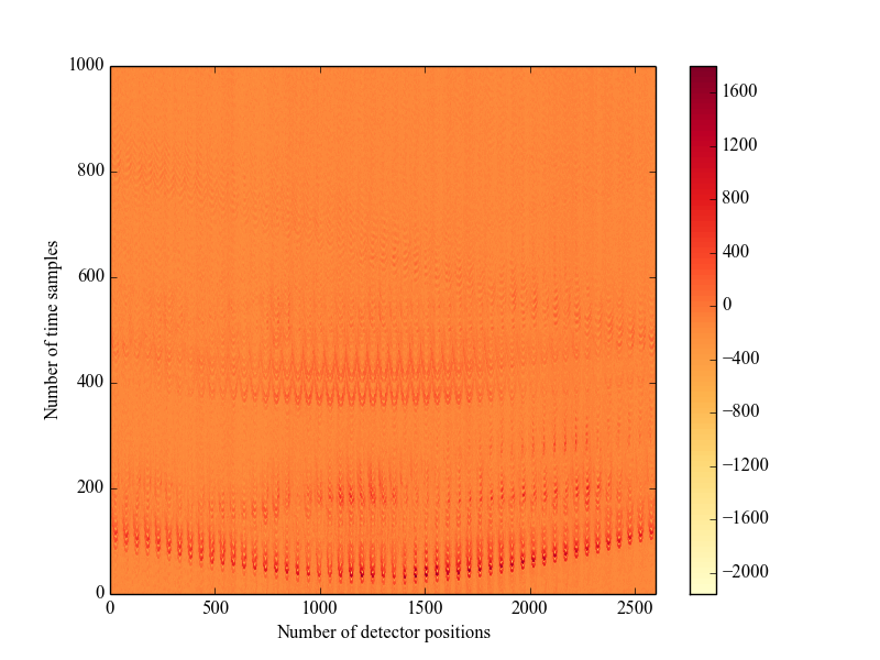
(a)

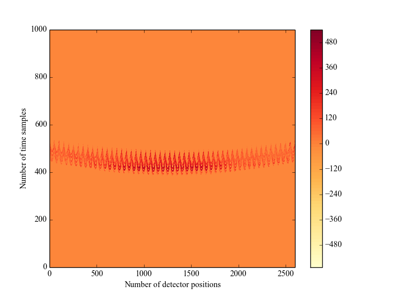
(b)

Figure 2: Experimental data before (a) and after steps 1-3 of the data prepocessing procedure (b).

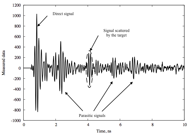
Figure 3: A typical sample of our time dependent experimental data.

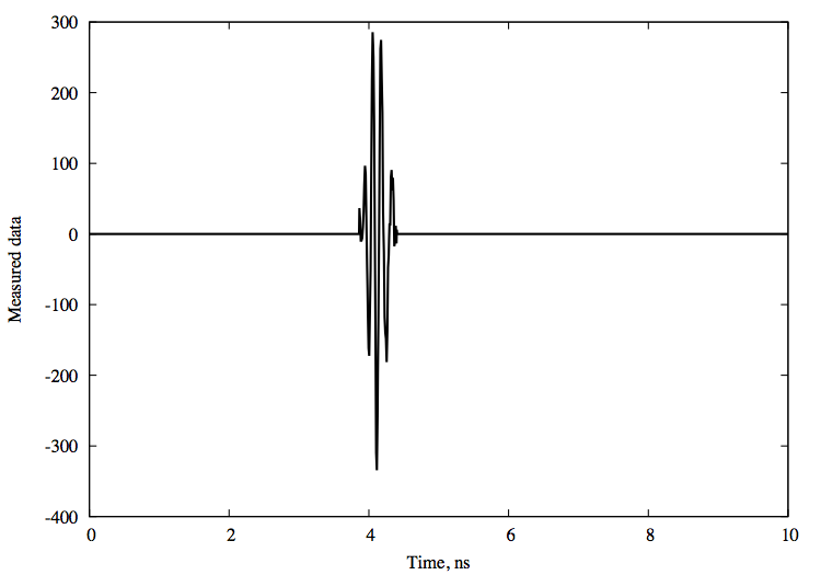
Figure 4: Preprocessed signal of Figure 3 after Steps 1-3.

4.2.5 Step 4. Fourier transform

Let $f(x,t)$ be the time dependent data obtained after above steps 1-3 of the data preprocessing. Following (10), we calculate the Fourier transform with respect to $t$,

$$\varphi(x,k)=\int_{0}^{\infty}f(x,t)\,e^{ikt}\,dt,\quad k\in[\underline{k},\overline{k}].$$

Since the data are measured on the rectangle $S_{m}=\left(-5,5\right)\times\left(-5,5\right)$ in the measurement plane, denoted by $P_{m}$, we set

$$f(x,t)=\varphi(x,k)=0,\quad\left(x_{1},x_{2}\right)\not\in S_{m}$$ (39)

Figure 5a shows $|\varphi(x,k)|$ $(k=13.5,$ see section 4.2.7$)$ for the experimental data for one of our targets on the measurement plane. Note that since the function $f(x,t)$ is extracted from the backscatter data, then the function $\varphi(x,k)$ also corresponds to the backscatter data rather than to a full wave field.

4.2.6 Step 5. Data propagation

The measurement plane was located quite far from the targets. This means that we were supposed to solve the CIP in a large domain, which is inconvenient. Besides, stability estimates for solving boundary value problems (3.2) and (34), (35) are worsened for large domains, as compared with smaller ones. The goal of the data propagation procedure is twofold: (a) To reduce the computational domain and (b) To make the data more “clear”, so that they the $x_{1},x_{2}$ coordinates of the targets would be clarified. The data propagation procedure is described in details in [32, 39]. Nevertheless, for the convenience of the reader, we briefly present the main steps below. This procedure is an application of the angular spectrum representation which is a well-known technique in the optics community, see [9, 32]. Basically, this procedure “moves” the data closer to the targets. The idea is that we consider the Helmholtz equation for the backscatter wave field outside the scattering medium. Then the Fourier transform with respect to $x_{1}$ and $x_{2}$ of the solution of this equation satisfies an ordinary differential equation in the $x_{3}$-direction. Together with the radiation condition and the boundary condition on the measurement plane one can solve that 1D problem and obtain the data on the propagated plane.

Let the measurement plane be $P_{m}=\{x_{3}=b\}$, $b>0$ and let $P_{p}=\{x_{3}=a\},a<b$ be the plane to which we want to propagate our data. We need to determine the function $u_{sc}\left(x,k\right)=\tilde{g}(x,k)$ on $P_{p},$ given the data $\varphi(x,k)$ on $P_{m}$. The computation consists of two steps. First, we compute the Fourier transform with respect to $x_{1}$ and $x_{2}$ of the function $\varphi(x,k)$ for $x\in P_{m},$

$$p(k_{1},k_{2},k)=\frac{1}{2\pi}\displaystyle\int\limits_{\mathbb{R}^{2}}\varphi(x,k)\,\exp\left(i\left(x_{1}k_{1}+x_{2}k_{2}\right)\right)\,dx_{1}dx_{2},$$

also see (39). In the second step, we apply the inverse Fourier transform, where the integration is carried out over a bounded domain $\left\{k_{1}^{2}+k_{2}^{2}<k^{2}\right\}.$ Denote $k_{z}=\sqrt{k^{2}-k_{1}^{2}-k_{2}^{2}}>0$. Then

$$u_{sc}\left(x,k\right)=\tilde{g}(x,k)=\frac{1}{2\pi}\int\limits_{k_{1}^{2}+k_{2}^{2}<k^{2}}p(k_{1},k_{2},k)\,e^{-i(x_{1}k_{1}+x_{2}k_{2}+(b-a)k_{z})}dk_{1}dk_{2},x_{3}=a.$$

We propagate our experimental data for all targets from the measurement plane $P_{m}=\{x_{3}=-8\}$ to the propagated plane $P_{p}=\{x_{3}=-0.75\}$. The functions $\left|\varphi(x,k)\right|$ and $\left|\tilde{g}(x,k)\right|$ for both simulated and experimental data at $k=13.5$ (see section 4.2.7) are displayed on Figures 5. This is the case of a single target, which is the target number 1, see Table 1 below. Figure 6 displays functions $\left|\varphi(x,k)\right|$ and $\left|\tilde{g}(x,k)\right|$ for the case of two inclusions for $k=15.1$ (see section 4.2.7). Most importantly, the data on the propagated plane are focused near the location of the target rather than being spread out as on the measurement plane. One can see on Figures 5b and 6b that we can now estimate $x_{1},x_{2}$ coordinates of targets, unlike Figures 5a and 6a. Furthermore, unlike the measurement plane of Figure 6a, two inclusions are clearly separated on the propagated plane of Figure 6b. Using these observations, we set

$$\tilde{g}(x,k)=0,\quad\mathrm{\ for}\ \left(x_{1},x_{2}\right)\notin S_{p}=\left(-2.5,2.5\right)\times\left(-2.5,2.5\right)\subset P_{p}.$$ (40)

4.2.7 Step 6. Choosing the interval for wave numbers

We now use temporary notations for numbers $\underline{k}$ and $\overline{k}$ as $\underline{k}^{\prime}$ and $\overline{k}^{\prime}$ respectively. We explain in this section how do we choose an appropriate interval $[\underline{k}^{\prime},\overline{k}^{\prime}]$ of wave numbers for each target. The interval of wave numbers should meet the following criteria:

1. The interval $[\underline{k}^{\prime},\overline{k}^{\prime}]$ contains the global maximizer of the function $s(k),$

   $$s(k)=\max_{x\in S_{p}}|\tilde{g}(x,k)|.$$ (41)

   Indeed, it seems to be intuitively at least that the data are most reliable for those values of wave numbers which are near that maximizer.

2. For $k\in[\underline{k}^{\prime},\overline{k}^{\prime}]$, the propagated data indicate correctly $x_{1},x_{2}$ coordinates of targets.

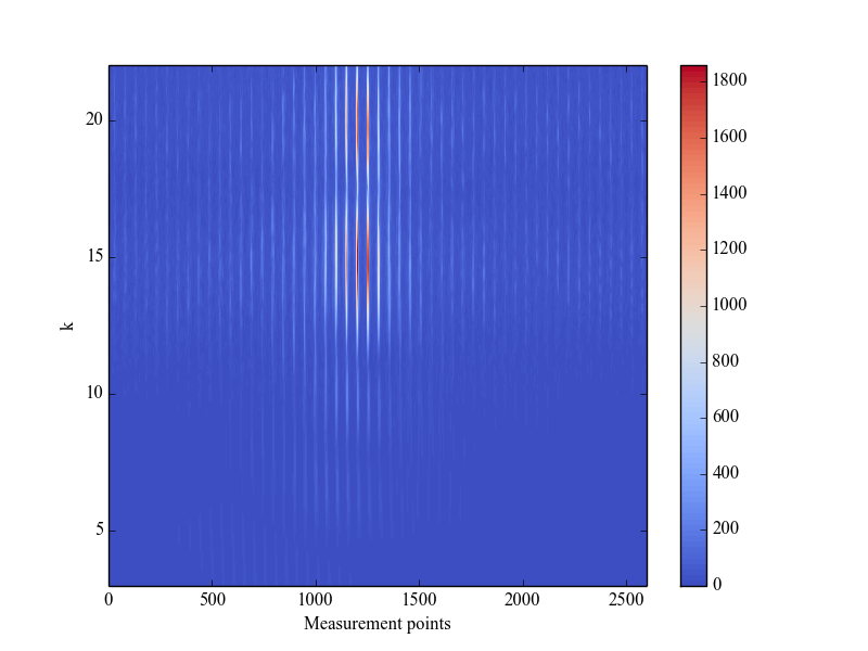
(b)

Figure 7: The graph of the function $s\left(k\right)$ defined in (41) for the reference target number 1. (b) The absolute value of the propagated experimental data. The horizontal line means grid points of the rectangle $S_{p}$ on the propagated plane $P_{p},$ see (40). The vertical axis denotes the wave numbers. We observe on (b) that the absolute values of the propagated data for $k\in[13.5,14]$ are near the maximal value of the function $|\tilde{g}(x,k)|$  and these data strongly focus in a subdomain of the rectangle $S_{p}$.

Here is an example. We plot on Figure 7a the graph of the function $s(k)$ defined in (41) for the target number 1 (see Table 1). This is our reference target for data calibration (see section 4.2.8). Since this is the reference target, we are supposed to know its location, shape and the value of its dielectric constant. We point out that this is unlike all other targets.

We observe on Figure 7a that $\max_{\left[0,20\right]}s\left(k\right)=s\left(13.75\right).$ Hence, the wave number $k=13.75$ is referred as the optimal frequency for the target number 1, see (38). Thus, we choose the interval of wave numbers for the target number 1 as $[\underline{k}^{\prime},\overline{k}^{\prime}]=[13.5,14]$ so that the optimal frequency is in the middle of this interval, $k_{opt}^{\prime}=\left(\underline{k}^{\prime}+\overline{k}^{\prime}\right)/2$. We choose the length of the $k-$interval to be the same for all targets, i.e. $a=\overline{k}^{\prime}-\underline{k}^{\prime}=0.5$. Figure 7b also confirms that this interval of wave numbers is optimal. It is clear from Figure 7b that the absolute values of the propagated data for $k\in[13.5,14]$ are near the maximal value of the function $|\tilde{g}(x,k)|$ and these data strongly focus in a subdomain of the rectangle $S_{p}$.

The interval $[13.5,14]$ of wave numbers corresponds to the interval of frequencies $\left[6.51,6.69\right]$ GHz. This can be converted to the interval of wavelengths $\lambda\in\left[0.0448,0.046\right]$ m. Note that the wave number interval for each target is different. The optimal frequency changes from 13.75 for the target number 1 to 18.7 for target number 9,

$$k_{opt}\in\left[13.75,18.7\right].$$ (42)

It is important to observe on Figure 7a that the function $s\left(k\right)$ changes slowly in the interval $[\underline{k}^{\prime},\overline{k}^{\prime}]=[13.5,14]$. On the other hand, it changes very rapidly for $k\in\left(11,\underline{k}^{\prime}\right)\cup\left(\overline{k}^{\prime},16\right),$ which is outside of the interval $[\underline{k}^{\prime},\overline{k}^{\prime}]$. Indeed, it changes between 200 and 1800 for $k\in\left(11,\underline{k}^{\prime}=13.5\right)$ and it changes between 1750 and 600 for $k\in\left(\overline{k}^{\prime}=14,16\right)$. Hence, we estimate the modulus of the derivative $\left|s^{\prime}(k)\right|$ as $\left|s^{\prime}(k)\right|>500$ for $k\in\left(11,\underline{k}^{\prime}\right)\cup\left(\overline{k}^{\prime},16\right).$ We consider this as an indication that the data are possibly highly unstable for $k\in\left(11,\underline{k}^{\prime}\right)\cup\left(\overline{k}^{\prime},16\right).$ Similar observations are true for the interval $k\in\left[16,20\right],$ which surrounds the local maximizer of $s\left(k\right)$ at $k=18.$ However, since $s\left(18\right)<s\left(13.75\right),$ then the first above criterion is not satisfied for $k\in\left[16,20\right].$ As to $k\in\left(0,11\right),$ we have observed that the second above criterion is not satisfied for our reference target number 1. Hence, we have ignored the interval $k\in\left(0,11\right)$ for this target. Also, because of this, we did the same for similar intervals for other targets without even checking the second criterion for them since we are not supposed to know locations of targets other than of the reference target. Thus, we work only on the interval $k\in[\underline{k}^{\prime},\overline{k}^{\prime}]=[13.5,14]$ for the target number 1 and on similar intervals for other targets.

However, the selected interval $[\underline{k}^{\prime},\overline{k}^{\prime}]=[13.5,14]$ of wave numbers is inconvenient for our computational purpose. The reason of this is that the solution $u\left(x,k\right)$ of the forward problem (2)-(5) is highly oscillatory for $k\in[13.5,14],$ so as for other intervals selected for other targets, see (42). This means that our solver for the Lippmann-Schwinger equation (11) requires a very fine mesh for these values of $k$ and thus, this solver becomes very expensive in terms of both the computing time and memory. On the other hand, we need to solve equation (11) on each iterative step of our algorithm to update the function $u\left(x,\overline{k}\right).$

Hence, we act as follows: In all our computations we use $k\in[\underline{k},\overline{k}]=[6,6.5]$ for all targets. However, for the data for the function $u_{sc}\left(x,k\right)$ on the propagated plane $P_{p}$ we use

$$u_{sc}\left(x,k\right):=\tilde{g}(x,k^{\prime}),k^{\prime}=k^{\prime}\left(k\right)=k+\underline{k}^{\prime}-6\in[\underline{k}^{\prime},\overline{k}^{\prime}],x\in S_{p},$$ (43)

also see (40). Thus, (43) means that we shift the data from the interval $[\underline{k}^{\prime},\overline{k}^{\prime}]=\left[\underline{k}^{\prime},\underline{k}^{\prime}+0.5\right]$ to the interval $[\underline{k},\overline{k}]=[6,6.5].$ In other words, even though the true data we work with are on the interval $[\underline{k}^{\prime},\overline{k}^{\prime}]$ of wave numbers, we pretend that they are on the interval $k\in[6,6.5].$

We have selected this $k-$interval since the same interval $[\underline{k},\overline{k}]=[6,6.5]$ was successfully used in the paper [30] of our group. The data shift was not performed in [30], since the optimal wave number of the data of [30] was inside the interval $[\underline{k},\overline{k}]=[6.25,6.70]$ for all targets. The latter corresponds to the interval of frequencies $\left[2.98,3.19\right]$ GHz.

Remark 4.1. Following (21), we have subdivided the interval $[6,6.5]$ in ten (10) subintervals with the step size $h=0.05$ and $N=10$. We point out that, in the case of the target number 1, even though the function (41) changes slowly on the interval $k\in[13.5,14],$ the function $|\tilde{g}(x,k)|$ might change rapidly with respect to $k$ for this $k-$interval at some points $x$. But at least the above considerations indicate that it seems to be meaningless to work on the intervals $k\in\left(0,13.5\right)$ and $k\in\left(14,16\right).$ The same procedure of the choice of the interval of wave numbers and of the data shift was performed for all targets used in our experiments. It follows from (42) that optimal intervals for different targets were different. See section 7 for our ultimate judgement of the validity of the entire data preprocessing procedure.

4.2.8 Step 7. Data calibration

We have observed that magnitudes of the experimental data are significantly different from magnitudes of computationally simulated data. For example, compare the absolute value of the Fourier transform of the experimental data on the propagated plane (Figure 5b) with the absolute value of propagated computationally simulated data on that plane (Figure 5d). The maximal value of propagated experimental data is about 950, whereas the maximal value of the propagated simulated data is about 0.28. Therefore, we need to scale the experimental data to the same scale as the one in computationally simulated data.

To do this, we consider one target, which we call “calibration target” (the target number 1) and consider the function $\tilde{g}(x,k+\underline{k}^{\prime}-6)$ for this target. Next, we compute the function $\varphi\left(x,k\right):=u\left(x,k\right)\mid_{x\in S_{m}\subset P_{m}},k\in[\underline{k},\overline{k}]=[6,6.5]$ (also, see (39)) on the measurement plane $P_{m}$ for a target, which mimics the target number 1: it has the same size, location and dielectric constant as the one of the target number 1. We compute the function $\varphi\left(x,k\right)$ via the numerical solution of the Lippmann-Schwinger equation (11) for this target. Next, we propagate the simulated data $\varphi\left(x,k\right)$ to the propagation plane $P_{p}$ and obtain the function $\tilde{g}_{sim}\left(x,k\right)$ this way.

Next, we define the $k-$dependent calibration factor $d(k)$ as

$$d(k)=\frac{\max_{S_{p}}(|\tilde{g}_{sim}(x,k)|)}{\max_{S_{p}}(|\tilde{g}(x,k+\underline{k}^{\prime}-6)|)},k\in[\underline{k},\overline{k}]=[6,6.5].$$ (44)

see (40) and (43). Once chosen, this function $d(k)$ remains the same for other targets. Using (44), we set for all targets

$$u\left(x,k\right) : =g\left(x,k\right)=\exp\left(ikx_{3}\right)+d\left(k\right)\tilde{g}(x,k+\underline{k}^{\prime}-6),$$ (45)

$$x \in S_{p}\subset P_{p},k\in[\underline{k},\overline{k}]=[6,6.5].$$

In this formula we multiply the experimental backscatter data by the calibration factor and then sum up with the incident wave. Note that it is not necessary of course that the calibration factor $d(k)$ defined in (44) using only one target would be perfect for other targets. Nevertheless, our reconstruction results below indicate that it works well. Similar considerations about the calibration factor are true for other studies of experimental data via GCM [7, 30, 38, 39].

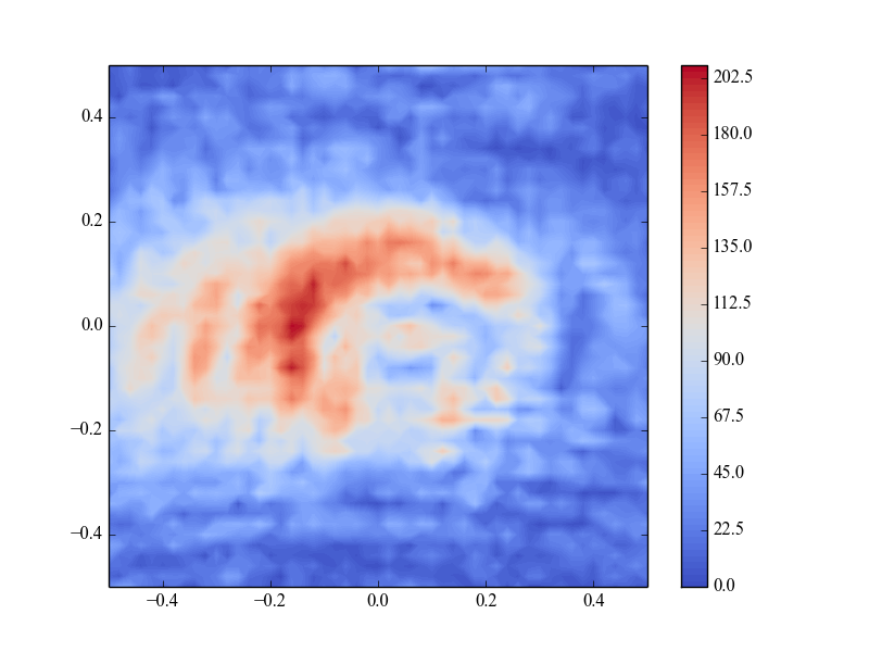
(a)

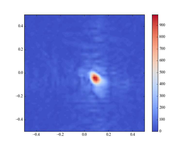
(b)

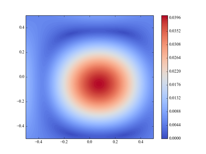
(c)

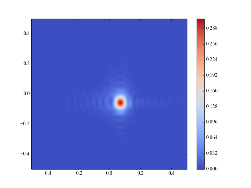
(d)

Figure 5: The absolute value of the Fourier transform of the preprocessed time dependent experimental data on the measurement plane (a) and the propagated plane (b). The absolute value of the Fourier transform of the computationally simulated data for the same target on the measurement plane (c) and on the propagated plane (d). $x_{1},x_{2}$ coordinates of the inclusion are clearly seen on (b) and (d), unlike (a) and (c). Here, $k=13.5$.

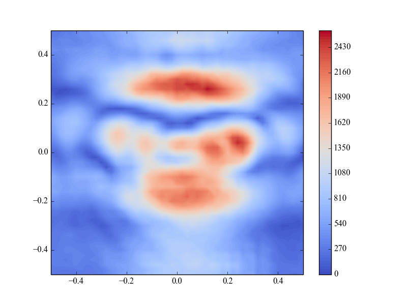
(a)

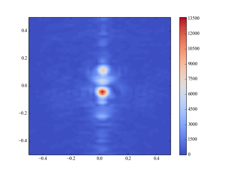
(b)

Figure 6: The absolute value of the Fourier transform of the experimental data for the case of two inclusions on the measurement plane (a) and on the propagated plane (b). $x_{1},x_{2}$ coordinates of both inclusions are clearly seen on (b), unlike (a). Here, $k=15.1$.

5 Numerical implementation

In this section, we describe some details of the numerical implementation of the algorithm described in section 3.2.

5.1 Computational domain

Recall that the $x_{3}$-axis in our coordinate system points from the measurement plane towards the target and the front face of the target is on the plane $\left\{x_{3}=0\right\}.$ We also recall that our propagated plane is $P_{p}=\left\{x_{3}=-0.75\right\}.$ We choose the computational domain $\Omega$ as:

$$\Omega=\{x\in(-2.5,2.5)\times(-2.5,2.5)\times(-0.75,4.25)\}.$$ (46)

The choice (46) means that the domain $\Omega$ is a cube whose side is 0.5 m. This is sufficient for our desired application since the linear sizes of antipersonnel mines and IEDs usually are between about 5 and 15 centimeters (cm). Observe that by the choice (46) we restrict our attention in planes, which are orthogonal to $x_{3},$ to rectangles $\left(x_{1},x_{2}\right)\in(-2.5,2.5)\times(-2.5,2.5),$ whereas the measured data are given on the rectangle $\left(x_{1},x_{2}\right)\in S_{m}=(-5,5)\times(-5,5)\subset P_{m}.$ This is because our propagated data are set to zero outside of the rectangle $S_{p}\subset P_{p},$ see (40). We solve Dirichlet boundary value problems (3.2) by the finite element method using the software FreeFem++ [19].

(a)

5.2 Complementing the backscatter data

Our backscatter experimental data are measured only on the rectangle $S_{m}$ of the measurement plane $P_{m}=\left\{x_{3}=-8\right\}$ and then are propagated to the plane $P_{p}=\left\{x_{3}=-0.75\right\}$. Hence, we denote

$$\Gamma=\partial\Omega\cap\left\{x_{3}=-0.75\right\}.$$

In fact, $\Gamma=S_{p}\subset P_{p}$. On the other hand, our algorithm of section 3.3 works only with the case when the data are given at the entire boundary $\partial\Omega.$ Thus, using (45), we complement the missing data on the rest of the boundary $\partial\Omega$ for $k\in\left[6,6.5\right]$ by the data in air $c(x)=1$

$$\widehat{g}(x,k)=\left\{\begin{array}[]{c}e^{ikx_{3}}+d\left(k\right)\tilde{g}_{exp}(x,k+\underline{k}^{\prime}-6),x\in\Gamma,\\ e^{ikx_{3}},x\in\partial\Omega\diagdown\Gamma.\end{array}\right.$$ (47)

This formula can be justified assuming that the targets are located far from $\partial\Omega\setminus\Gamma$ and the influence of waves scattered from $\partial\Omega\setminus\Gamma$ is small. We note that in the above cited references [7, 25, 30, 38, 39] the backscatter data were complemented the same way as in (47). The $k-$derivative $\partial_{k}\tilde{g}_{exp}$ was found using the finite difference method with the step size $h=0.05$, which is the same as in Remark 4.1. Even though the differentiation of noisy data is an ill-posed problem, we have not observed any instabilities. This is because of the efficiency of the data propagation and the choice of the optimal interval of wave numbers. Note that a similar differentiation procedure, although with respect to the parameter of the Laplace transform, was applied in [5, 6] to computationally simulated data with noise and to experimental data in [7, 38, 39]. In the case of the differentiation with respect to $k$, it was also applied in [25, 30]. It was stable in all cases. A further study of the differentiation topic is outside of the scope of this paper.

5.3 The first tail function $V_{0}\left(x\right)$

Since we set $\Delta V_{0}=0$ (section 3.4), then it is clear from (3.2) (at $n=1$) that we use only the gradient $\nabla V_{0}$ of the first tail function $V_{0}$. Thus, to avoid the error associated with the numerical differentiation of the first tail function $V_{0}(x)$, we numerically solve the following problem instead of the problem (34), (35)

$$\Delta(\partial_{x_{j}}V_{0})=0,\quad x\in\Omega.$$

$$\partial_{x_{j}}V_{0}=\frac{\partial_{x_{j}}u(x,\overline{k})}{u(x,\overline{k})},\quad x\in\Gamma,\quad j=1,2,3,$$ (48)

$$\partial_{x_{j}}V_{0}=0,\quad j=1,2,\quad x\in\partial\Omega\setminus\Gamma,$$ (49)

$$\partial_{x_{3}}V_{0}=i\overline{k},\quad x\in\left\{x_{3}=4.25\right\}\cap\partial\Omega.$$ (50)

We now comment about boundary conditions (48)-(50). Conditions (48) follow from (19), (20), (26) and (35). Conditions (49) and (50) for $x\in\left\{x_{3}=4.25\right\}\cap\partial\Omega$ follow from our assumption in the second line of (26). In addition, conditions (49) are approximate ones for those parts of the rest of $\partial\Omega\setminus\Gamma$ which are orthogonal to the $x_{j}-$axis. In the latter case they basically mean that the function $V_{0}$ does not change in the direction $x_{j}$ near of those parts of the boundary. As to condition (48), it implies that we need the boundary data for functions $\partial_{x_{j}}u(x,\overline{k})$, $x\in\Gamma,$ $j=1,2,3$. The derivatives with respect to $x_{1}$ and $x_{2}$ are found by differentiating $g(x,\overline{k})$ which is defined in (45). The derivative with respect to $x_{3}$ for $x\in\Gamma$ is calculated as

$$\partial_{x_{3}}u(x,\overline{k})=d(\overline{k})\partial_{x_{3}}\tilde{g}(x,\overline{k})+i\overline{k}\exp(i\overline{k}x_{3}),$$

where $\partial_{x_{3}}\tilde{g}(x,\overline{k})$ is the derivative of the propagated experimental data $\tilde{g}(x,\overline{k})$ with respect to $x_{3}$. The function $\partial_{x_{3}}\tilde{g}(x,\overline{k})$ was found by propagating the Fourier transform of experimental data to the two nearby planes $P_{p}=\{x_{3}=-0.75\}$ and $P_{p_{\varepsilon}}=\{x_{3}=-0.75+\varepsilon\}$, subtracting the results from each other and dividing by $\varepsilon$, where we took $\varepsilon=0.1$. Derivatives $\partial_{x_{j}}g(x,\overline{k}),j=1,2$ for $x\in\Gamma$ were found using FreeFEM++ and Matlab. The preprocessed data looked very smooth and we have not observed any instabilities.

5.4 Truncation

As it is clear from results of data propagation (Figures 5b,d and 6b), $x_{1},x_{2}$ coordinates of targets can be estimated from images on the propagated plane $P_{p}$. We have observed for all targets of our study that the absolute value of the Fourier transform of the propagated experimental data $\tilde{g}(x,k)$ has a positive peak (see, e.g. Fig. 5b), which corresponds to the $x_{1},x_{2}$ location of a target. Thus, we define the set $\Gamma_{t}\subset S_{p}$ as

$$\Gamma_{t}=\left\{(x_{1},x_{2}):|\tilde{g}(x,\overline{k})|>0.7\max|\tilde{g}(x,\overline{k})|,(x_{1},x_{2})\in S_{p}\right\}.$$

Here, the truncation value 0.7 is chosen by trial and error as an optimal number.

Taking into account our desired application to detection and identification of explosives, we look for our targets only in the interval $(-0.75,1)$ in the $x_{3}-$direction. This means that we allow the maximal linear size of the target in the $x_{3}$-direction to be 17.5 cm, which is close to the upper bound of about 15 cm for antipersonnel mines and IEDs. Recall that the function $c_{n,i}(x)$ is calculated by formula (24) in our algorithm. However, the right hand side of this formula might be complex valued. Hence, we need to postprocess (24). So, we define the postprocessed function $c_{n,i}^{\left(p\right)}(x)$ as:

$$c_{n,i}^{\left(p\right)}(x)=\left\{\begin{array}[]{cc}\left|c_{n,i}(x)\right|,&\quad x\in\Gamma_{t}\times(-0.75,1.0),\\ 1,&\quad\mbox{elsewhere},\end{array}\right.$$ (51)

where $c_{n,i}(x)$ is the function calculated by (24). Next, the coefficient $c_{n,i}^{\left(p\right)}$ is smoothed by the smooth3 function in Matlab. That smoothed coefficient is used then to solve the Lippmann-Schwinger equation in our algorithm.

In the case of targets with two inclusions, their $x_{1},x_{2}$ coordinates are seen on the propagated plane $P_{p}$. However, the signal from one inclusion might be stronger than from the other, see Fig. 6b. This might mean that either one inclusion has a larger dielectric constant than the second one, or perhaps they have different volumes, or both. Thus, it is hard to reconstruct both the “stronger” and the “weaker” inclusions simultaneously. Therefore, we treat these inclusions as two separate targets. For example, in Fig. 6b we consider the median straight line on the plane $P_{p}$ between images of these two inclusions on $P_{p}$. Next, to image the top inclusion, we set the propagated data below this line to be zero $\tilde{g}(x,k):=0$. Next, we apply the above procedure, which gives us the image of the top inclusion. Having the image of the top inclusion, we then set $\tilde{g}(x,k):=0$ for points $x\in P_{p}$ located above that median line and repeat. Finally we combine two images in one. The reconstruction results for both inclusions look good and their $x_{3}-$locations are the same as it should be, see Figures 11 and 12.

6 Reconstruction results

The preprocessed experimental data (47), as well as the gradient of the first tail function, which was calculated as in section 5.3, were used as the input for our globally convergent algorithm of subsection 3.3. We present in this section results of the reconstructions by this algorithm.

We have considered ten (10) data sets. In seven cases we had one target, and we had two targets in the rest of three data sets. Six targets were dielectrics, three were metallic ones and one target was a mixture of a wood and metal. Although the dielectric constant of the metal is not well-defined, it was established in an earlier work [27] that, in the case of metallic targets, one can assume that they have large the so-called appearing dielectric constants,

$$c\left(\mbox{metal}\right)\in\left[10,30\right].$$ (52)

A description of targets and their linear sizes is given in Table 1. Recall that the target number 1 was chosen as the reference object for data calibration.

Target	Description	Size in cm,
number		($x_{1}\times x_{2}\times x_{3}$)
1	A piece of oak	$4.1\times 8.2\times 4.1$
2	Metallic ball	$10.3\times 10.3\times 10.3$
3	Metallic cylinder	$5.3\times 11.1\times 5.3$
4	Wooden object	$6.0\times 11.3\times 4.0$
5	Wooden doll with air inside	$8.7\times 11.5\times 8.7$
6	Wooden doll with metal inside	$8.7\times 11.5\times 8.7$
7	Wooden doll filled with sand	$8.7\times 11.5\times 8.7$
8	Two metallic objects	$5.5\times 10.1\times 2.5$
		$5.9\times 4.1\times 4.1$
9	Two wooden objects aligned vertically	$9.6\times 5.8\times 5.3$
		$11.3\times 6.0\times 3.3$
10	Two wooden objects aligned horizontally	$4.1\times 8.15\times 4.1$
		$5.7\times 9.7\times 5.7$

Table 1: Targets and their linear sizes in centimeters

We choose the final reconstructed coefficient as follows. First, we calculate the following relative errors

$$\varepsilon_{n,i}=\left\{\begin{array}[]{c}\frac{\|c_{n,i}-c_{n,i-1}\|_{L_{2}(\Omega)}}{\|c_{n,i-1}\|_{L_{2}(\Omega)}},\mbox{ for }i=2,...m,\,1\leq n\leq N=10,\\ \frac{\|c_{n+1,1}-c_{n}\|_{L_{2}(\Omega)}}{\|c_{n}\|_{L_{2}(\Omega)}},\mbox{ for }i=1,\,1\leq n\leq N=9.\end{array}\right.$$ (53)

Suppose that the minimal error out of numbers (53) is achieved at $n=n_{0},i=i_{0}.$ Then we set the computed coefficient $c_{comp}\left(x\right)=c_{n_{0}i_{0}}\left(x\right).$ If the minimal error is achieved for several pairs $\left(n,i\right),$ then we choose the pair $\left(n_{0},i_{0}\right)$ which was the first one in (53). Note that the number of inner iterations in our computations is $m=3$. This number was chosen by trial and error.

To verify the accuracy of our computations, we have a posteriori measured directly refractive indices $n=\sqrt{c}$ of our six dielectric targets. Since the latter measurements were in time domain, the dependencies of measured indices on the frequency were not known, but we believe that approximating it by a constant in the small intervals of wave numbers we work with is reasonable. In table 2 we present the measured and computed refractive indices of the dielectric targets together with the errors in their measurements and computational errors. The computed value of refractive index is defined as $n_{comp}=\sqrt{\max_{\overline{\Omega}}c_{comp}(x)}$ and its error is computed as

$$\varepsilon_{comp}=\frac{\left|n_{true}-n_{comp}\right|}{n_{true}}100\%.$$

Table 2 demonstrates that our computational results for refractive indices of dielectric targets are highly accurate. Indeed, the computational errors are smaller than the corresponding measurement errors. In fact, the error for the reference target 1 is the smallest one, which indicates that the experimental data for this target were correctly scaled using the calibration factor (44). We also observe that the computational errors for the second object of data sets 9 and 10 are higher than the errors for the first object in the same data set. This can be explained by the fact that the second objects in these data sets have smaller refractive indices. Hence, their the reflected signals are weaker than ones of first objects, which, in turn leads to a higher computational error.

Recall that we associate the so-called appearing dielectric constant with metals, see (52). Thus, we model metallic targets as the dielectric targets with high values of the dielectric constant $c\in[10,30]$. In table 3 we present the computed appearing dielectric constants $c_{c}=\max_{\overline{\Omega}}c_{comp}(x)$ for our metallic targets. We see that the computed appearing dielectric constant $c_{c}=6.68$ of the target number 2 is less than 10. This is because the signal reflected by this target is not strong enough. Indeed, for this target, the maximal absolute value of the preprocessed time dependent signal after Step 3 was about 800. On the other hand, the analogous value for targets number 3 and 8 were about 1800 and 3200, respectively.

The maximal absolute value of the preprocessed time dependent signal after Step 3 for the target number 6 was about 1100, which is also significantly less than this value for targets number 3 and 8. The computed appearing dielectric constant 9.73 of the target number 6 is close to the lower limit of 10. It is natural, however, that it is lower than 10, since a piece of metal in this target was covered by the surface of that wooden doll. The latter, in turn has caused the decrease of that maximal absolute value.

Figures 8 – 12 illustrate the true and computed images for the targets number 1, 3, 5, 8, 10. We use isosurfaces of Matlab to draw these figures. Reconstructed images for the rest of five targets with numbers 2, 4, 6, 7, 9 are similar. We see that the positions of objects are imaged correctly. Shapes are not well reconstructed. Still, in the case of two objects of target number 10 (Fig. 12a), one object is larger than another one, and we observe the same on computed objects (Fig. 12b), which is accurate. In the case of the wooden doll with air inside of the object number 5 (Fig. 10a), only its larger part is reconstructed, which is natural.

Target	Refractive index
number	Measured value $n_{true}$ (error, %)	Computed value $n_{comp}$ (error, %)
1	2.11     (19)	2.08     (1.39)
4	2.14     (28)	2.54     (18.8)
5	1.89     (30)	2.06     (8.99)
7	2.10     (26)	2.28     (8.38)
9	2.14     (18)	2.25     (5.21)
	1.84     (18)	2.03     (10.3)
10	2.14     (18)	2.28     (6.48)
	1.84     (18)	2.08     (13.3)

Table 2: Measured and computed refractive indices of dielectric targets.

Target	Computed appearing dielectric constant $c_{comp}\quad$
number
2	6.68
3	11.49
6	9.73
8	18.47
	18.73

Table 3: Computed appearing dielectric constants of metallic targets

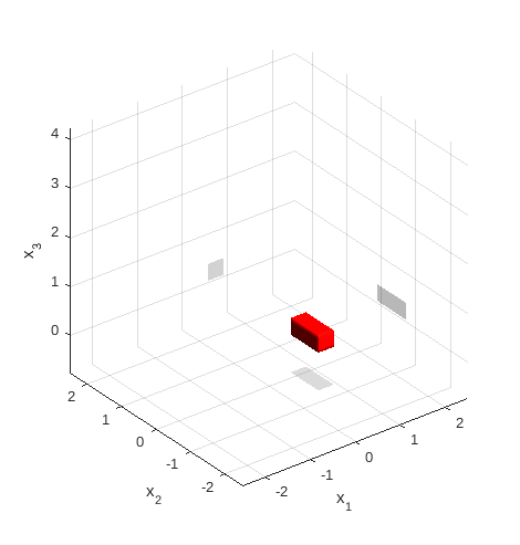
(a)

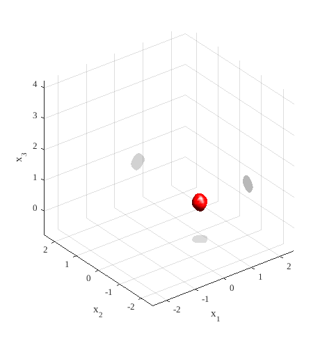
(b)

Figure 8: Reconstruction result for the target number 1: true image (a) and computed image (b).

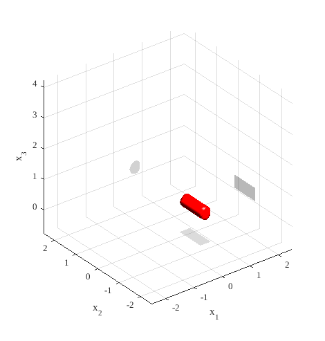
(a)

(b)

Figure 9: Reconstruction result for the target number 3: true image (a) and computed image (b).

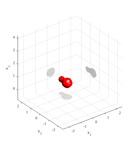
(a)

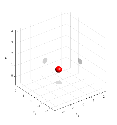
(b)

Figure 10: Reconstruction result for the target number 5: true image (a) and computed image (b).

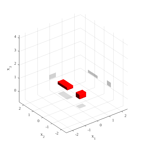
(a)

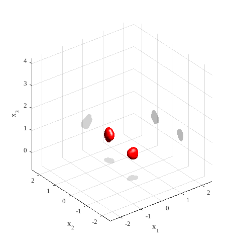
(b)

Figure 11: Reconstruction result for the target number 8: true image (a) and computed image (b).

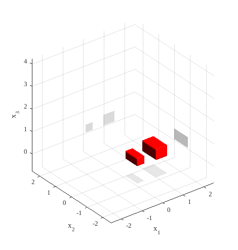
(a)

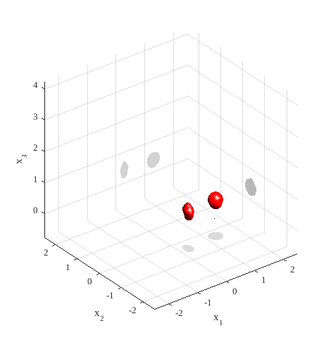
(b)

Figure 12: Reconstruction result for the target number 10: true image (a) and computed image (b). Note that the computed image corresponding to the inclusion of a larger size on (a) is indeed larger on (b).

7 Discussion

In this paper, we have tested the performance of the GCM of [25] on time dependent experimental data. Since the technique of [25] works for multi-frequency data, we have applied the Fourier transform to preprocessed time dependent data. The main difficulty working with the data of both the current paper and [30] was a huge discrepancy between these data and computationally simulated ones. Standard denoising techniques do not work for this case due to a richer content of the real data, compared with the computationally simulated ones. Thus, we have developed here a heuristic data preprocessing procedure. The resulting data look somehow similar to the computationally simulated ones. These preprocessed data are used then as the input for the GCM.

Our data preprocessing procedure consists of two stages. On the first stage, the time dependent data are preprocessed. On the second stage, the Fourier transform is applied to the data preprocessed on the first stage, and then the resulting data are preprocessed again in the frequency domain. Even though the first stage is similar with [38] and the second stage is similar with [30], there are two important differences with these two references: one difference in each stage. The difference in the first stage is caused by the difference between the Fourier transform used in the current publication and the Laplace transform used in [38]. The difference in the second stage is in the data shift (43), which was not used in [30]. This data shift is caused by the difference between our Fourier transformed data and the multi-frequency experimental data of [30].

Some elements of our heuristic data preprocessing procedure might seem to be of a concern, such as, e.g. formula (43). However, we believe that the ultimate judgement about the usefulness of this procedure as a whole should be drawn on the basis of obtained reconstruction results. As to the latter, it is clear from table 2 that numerical results of reconstructions of refractive indices of dielectric targets are very accurate. Furthermore, they are even significantly more accurate than results of direct measurements of $n$. Recall that refractive indices $n$, rather than dielectric constants $c=n^{2}$ were a posteriori directly measured in our experiments. We also recall that it is hard for optimization methods for CIPs to accurately calculate values of unknown coefficients inside the targets.

Table 3 demonstrates that appearing dielectric constants $c$ of metallic targets number 3 and 8 are also in the required range of $c\in\left[10,30\right],$ see (52). Although the computed value $c_{c}=6.68$ for the metallic target number 2 is less than 10, it is still quite high, as compared with dielectric constants of non metallic targets in table 2, all of which do not exceed 2.6. As it was explained in section 6, the reason why the computed appearing dielectric constant of target number 2 is significantly less than 10 is that the preprocessed time dependent signal after Step 3 for this case was significantly weaker than the one for the targets number 3 and 8.

The fact that the computed appearing dielectric constant $c_{c}=9.73$ of the target number 6 is less than 10 has a natural explanation. Indeed, this target is a piece of metal hidden inside of an otherwise empty wooden doll, see Table 1. Therefore, the surface of this doll works as a “mask” for that metal. This observation seems to be of an interest for our desired application to imaging of mines and IEDs.

Locations of all targets are imaged accurately. Although shapes are computed inaccurately, in the case of two objects of Figure. 12a, the smaller object is computed as the smaller one, see Figure 12b.

The main advantage of our GCM is that, given a reasonable mathematical assumption, there is a rigorous guarantee that it provides some points in a small neighborhood of the exact coefficient [25]. This is an important difference compared with conventional optimization methods. A reasonable mathematical assumption seems to be unavoidable due to the well known fact that the development of globally convergent numerical methods for CIPs, all of which are highly nonlinear, is a substantially challenging task, especially in the case of single measurement data. Our reasonable mathematical assumption is (28) and (29), which amounts to ignoring the small term $O(1/k)$ in (26). That assumption is used only once: for defining the first tail function $V_{0}.$ However, it is not used on follow up iterations of our numerical method.

One of conditions of the  global convergence theorem for our GCM [25] is that the interval $\left[\underline{k},\overline{k}\right]$ of wave numbers should be sufficiently small, so as the discretization step size $h$ with respect to $k$. Interestingly, this is exactly the case of our data, so as of the data of [30]. Indeed, consider the relative length of this interval $a=\left(\overline{k}-\underline{k}\right)/\underline{k}.$ Then in our case $a=0.5/6=0.083$ after the data shift (43) (see section 4.2.7). Hence, in our case $h=0.0083=0.083/10.$ Both these numbers are sufficiently small. In addition, the analysis of section 4.2.7 indicates that it is likely meaningless to work on a larger interval of wave numbers. This provides a sort of a justification of that smallness condition from the Physics standpoint.

Acknowledgements

This work was supported by the US Army Research Laboratory and US Army Research Office grant W911NF-15-1-0233 as well as by the Office of Naval Research grant N00014-15-1-2330.

References

References

- [1] A. D. Agaltsov. Finding scattering data for a time-harmonic wave equation with first order perturbation from the dirichlet-to-neumann map. J. Inverse and Ill-Posed Problems, 23:627–645, 2015.
- [2] A. D. Agaltsov and R. G. Novikov. Riemann–hilbert problem approach for two-dimensional flow inverse scattering. J. Mathematical Physics, 55:103502, 2014.
- [3] H. Ammari, Y. T. Chow, and J. Zou. Phased and phaseless domain reconstruction in inverse scattering problem via scattering coefficients. SIAM J. Appl. Math, 76:1000–1030, 2016.
- [4] G. Bao, P. Li, J. Lin, and F. Triki. Inverse scattering problems with multi-frequencies. Inverse Problems, 31(9):093001, 21, 2015.
- [5] L. Beilina and M. V. Klibanov. Approximate Global Convergence and Adaptivity for Coefficient Inverse Problems. Springer, New York, 2012.
- [6] L. Beilina and M. V. Klibanov. A new approximate mathematical model for global convergence for a coefficient inverse problem with backscattering data. J. Inverse and Ill-Posed Problems, 20:512–565, 2012.
- [7] L. Beilina, N. T. Thành, M. V. Klibanov, and M. A. Fiddy. Reconstruction from blind experimental data for an inverse problem for a hyperbolic equation. Inverse Problems, 30(2):025002, 2014.
- [8] M. I. Belishev, I. B. Ivanov, I. V. Kubyshkin, and V. S. Semenov. Numerical testing in determination of sound speed from a part of boundary by the bc-method. J. Inverse and Ill-Posed Problems, 24:159–180, 2016.
- [9] M. Born and E. Wolf. Principles of Optics: Electromagnetic Theory of Propagation, Interference and Diffraction of Light. Cambridge University Press, 7 edition, 1999.
- [10] A. L. Bukhgeim and M. V. Klibanov. Global uniqueness of a class of multidimensional inverse problems. Soviet Mathematics Doklady, 24:244–247, 1981.
- [11] F. Cakoni and D. Colton. Qualitative Methods in Inverse Scattering Theory. An Introduction. Springer, Berlin, 2006.
- [12] G. Chavent. Nonlinear Least Squares for Inverse Problems: Theoretical Foundations and Step-by-Step Guide for Applications (Scientific Computation). Springer, New York, 2009.
- [13] Y. Chen. Inverse scattering via Heisenberg’s uncertainty principle. Inverse Problems, 13(2):253–282, 1997.
- [14] W.C. Chew and J.H. Lin. A frequency-hopping approach for microwave imaging of large inhomogeneous bodies. IEEE Microwave and Guided Wave Letters, 5:439–441, 1995.
- [15] D.L. Colton and R. Kress. Inverse acoustic and electromagnetic scattering theory. Applied Mathematical Sciences. Springer, 2 edition, 1998.
- [16] M. Dorn and D. Lesselier. Level set methods for structural inversion and image reconstruction. In O. Scherzer, editor, Handbook of Mathematical Methods in Imaging, pages 471–532. Springer, 2015.
- [17] J. M. Geffrin and P. Sabouroux. Continuing with the fresnel database: experimental setup and improvements in 3d scattering measurements. Inverse Problems, 25(2):024001, 2009.
- [18] R. Griesmaier. Multi-frequency orthogonality sampling for inverse obstacle scattering problems. Inverse Problems, 27(8):085005, 23, 2011.
- [19] F. Hecht. New development in FreeFem++. J. Numer. Math., 20:251–265, 2012.
- [20] I. B. Ivanov, M. I. Belishev, and V. S. Semenov. The reconstruction of sound speed in the marmousi model by the boundary control method. arXiv:1609.07586, 2016.
- [21] S. I. Kabanikhin, K. K. Sabelfeld, N. S. Novikov, and M.A Shishlenin. Numerical solution of the multidimensional gelfand-levitan equation. J. Inverse and Ill-Posed Problems, 23:439–450, 2015.
- [22] S. I. Kabanikhin, A. D. Satybaev, and M.A Shishlenin. Direct methods of solving multidimensional inverse hyperbolic problem. VSP, Utrecht, 2004.
- [23] A. Kirsch and N.I. Grinberg. The Factorization Method for Inverse Problems. Oxford Lecture Series in Mathematics and its Applications 36. Oxford University Press, 2008.
- [24] M. V. Klibanov. Carleman estimates for global uniqueness, stability and numerical methods for coefficient inverse problems. J. Inverse and Ill-Posed Problems, 21(4):477–560, 2013.
- [25] M. V. Klibanov, H. Liu, and L. H. Nguyen. A globally convergent method for a 3-D inverse medium problem for the generalized helmholtz equation. arxiv:1605.06147, 2016.
- [26] M. V. Klibanov and V. G. Romanov. Two reconstruction procedures for a 3d phaseless inverse scattering problem for the generalized helmholtz equation. Inverse Problems, 32:015005, 2016.
- [27] A. V. Kuzhuget, L. Beilina, M. V. Klibanov, A. Sullivan, L. Nguyen, and M. A. Fiddy. Blind backscattering experimental data collected in the field and an approximately globally convergent inverse algorithm. Inverse Problems, 28(9):095007, 2012.
- [28] J. Li, H. Liu, and J. Zou. Locating multiple multiscale acoustic scatterers. SIAM Multiscale Model. Simul, 12:927–952, 2014.
- [29] A. Litman and L. Crocco. Testing inversion algorithms against experimental data: 3d targets. Inverse Problems, 25(2):020201, 2009.
- [30] D.-L. Nguyen, M. V. Klibanov, L. H. Nguyen, A. E. Kolesov, M. A. Fiddy, and H. Liu. Experimental multi-frequency data for a globally convergent numerical method for an inverse scattering problem. arxiv:1609.03102, 2016.
- [31] R. G. Novikov. An iterative approach to non-overdetermined inverse scattering at fixed energy. Sbornik: Mathematics, 206:120–134, 2015.
- [32] L. Novotny and B. Hecht. Principles of Nano-Optics. Cambridge University Press, 2 edition, 2012.
- [33] R. Potthast. A survey on sampling and probe methods for inverse problems. Inverse Problems, 22:R1–R47, 2006.
- [34] R. Potthast. A study on orthogonality sampling. Inverse Problems, 26:074015(17pp), 2010.
- [35] M. Sini and N. T. Thành. Inverse acoustic obstacle scattering problems using multifrequency measurements. Inverse Problems and Imaging, 6:749–773, 2012.
- [36] M. Sini and N. T. Thành. Regularized recursive newton-type methods for inverse scattering problems using multifrequency measurements. ESAIM Math. Model. Numer. Anal., 49:459–480, 2015.
- [37] M. Soumekh. Synthetic Aperture Radar Signal Processing. John Wiley & Son, New York, 1999.
- [38] N. T. Thành, L. Beilina, M. V. Klibanov, and M. A. Fiddy. Reconstruction of the refractive index from experimental backscattering data using a globally convergent inverse method. SIAM Journal on Scientific Computing, 36(3):B273–B293, 2014.
- [39] N. T. Thành, L. Beilina, M. V. Klibanov, and M. A. Fiddy. Imaging of buried objects from experimental backscattering time dependent measurements using a globally convergent inverse algorithm. SIAM J. on Imaging Sciences, 8(1):757–786, 2015.
- [40] A. N. Tikhonov, A. V. Goncharsky, V. V. Stepanov, and A. G. Yagola. Numerical Methods for the Solution of Ill-Posed Problems. Springer, 1995.
- [41] B.R. Vainberg. Asymptotic Methods in Equations of Mathematical Physics. Gordon and Breach Science, New York, 1989.
- [42] G. Vainikko. Fast Solvers of the Lippmann-Schwinger Equation, pages 423–440. Springer, Boston, 2000.
- [43] M. Yamamoto. Carleman estimates for parabolic equations and applications. Inverse Problems, 25(12):123013, 2009.
- [44] O. Yilmaz. Seismic Data Imaging. Society of Exploration Geophysicists, Tulsa Oklahoma, 1987.