Energy and periastron advance of compact binaries
on circular
orbits at the fourth post-Newtonian order
Abstract
In this paper, we revisit and complete our preceding work on the Fokker Lagrangian describing the dynamics of compact binary systems at the fourth post-Newtonian (4PN) order in harmonic coordinates. We clarify the impact of the non-local character of the Fokker Lagrangian or the associated Hamiltonian on both the conserved energy and the relativistic periastron precession for circular orbits. We show that the non-locality of the action, due to the presence of the tail effect at the 4PN order, gives rise to an extra contribution to the conserved integral of energy with respect to the Hamiltonian computed on shell, which was not taken into account in our previous work. We also provide a direct derivation of the periastron advance by taking carefully into account this non-locality. We then argue that the infra-red (IR) divergences in the calculation of the gravitational part of the action are problematic, which motivates us to introduce a second ambiguity parameter, in addition to the one already assumed previously. After fixing these two ambiguity parameters by requiring that the conserved energy and the relativistic periastron precession for circular orbits are in agreement with numerical and analytical gravitational self-force calculations, valid in the limiting case of small mass ratio, we find that our resulting Lagrangian is physically equivalent to the one obtained in the ADM Hamiltonian approach.
pacs:
04.25.Nx, 04.30.-w, 97.60.Jd, 97.60.LfI Introduction
This paper is a follow up to Ref. Bernard et al. (2016a), in which we derived the equations of motion of compact binary systems (without spins) at the 4PN approximation of general relativity.111We shall refer to Ref. Bernard et al. (2016a) as “Paper I” henceforth. As usual the PN order corresponds to post-Newtonian corrections up to order beyond the Newtonian acceleration in the equations of motion. In Paper I, we gave a short account of numerous past works on the PN equations of motion of compact binaries (see Blanchet (2014) for a more exhaustive review). At the 3PN order, the equations were independently derived using different methods: Hamiltonian formalism Jaranowski and Schäfer (1998, 1999, 2000); Damour et al. (2000, 2001a, 2001b), harmonic coordinates approach Blanchet and Faye (2000a, 2001, b); de Andrade et al. (2001); Blanchet and Iyer (2003); Blanchet et al. (2004), surface-integral method Itoh et al. (2000, 2001); Itoh and Futamase (2003); Itoh (2004); Futamase and Itoh (2007), and effective field theory (EFT) Foffa and Sturani (2011).
At the 4PN order, partial results were first obtained within the Hamiltonian formalism in ADM-like coordinates Jaranowski and Schäfer (2012, 2013, 2015) and the EFT approach Foffa and Sturani (2012). The 4PN Hamiltonian was then completed in Refs. Damour et al. (2014, 2016) by adding a non-local (in time) contribution related to gravitational-wave tails, known from Refs. Blanchet and Damour (1988); Blanchet (1993) for general matter systems. An alternative derivation of the 4PN dynamics, including the same non-local tail piece, was achieved in Paper I by computing the Fokker Lagrangian in harmonic coordinates. This result agreed with the partial results of the EFT Foffa and Sturani (2012), and also with most of the terms in the 4PN Hamiltonian Jaranowski and Schäfer (2012, 2013, 2015); Damour et al. (2014, 2016). However, it disagreed with a few terms [see Eqs. (5.18)–(5.19) in Paper I]. Part of the discrepancy was due to the fact that Refs. Damour et al. (2014, 2016) and Paper I use different prescriptions to handle the non-local tail term, as discussed in Sec. VC of Paper I and in more details below.
An important point of comparison for the PN results is given by gravitational self-force (GSF) calculations, valid in the small mass ratio limit (see Refs. Detweiler (2011); Barack (2011) for reviews). The recent years have seen a lot of progress on numerical or analytical calculations of two gauge-invariant quantities, the conserved energy and the advance of the periastron for circular orbits, allowing for unambiguous comparisons with the small mass-ratio limit of the PN results. The GSF energy for circular orbits has been computed numerically in Blanchet et al. (2010); Le Tiec et al. (2012a, b) and analytically (in the form of a PN expansion) in Bini and Damour (2013), while the circular orbit limit of the periastron advance has been obtained numerically in Barack et al. (2010); Le Tiec et al. (2011); van de Meent (2016) and analytically in Damour (2010); Damour et al. (2015, 2016). The GSF calculations of the energy and periastron advance generally rely on the so-called first law of black hole binaries Le Tiec et al. (2012a); Le Tiec (2015), which was initially derived at 3PN order, but has recently been shown to be valid at the 4PN order, taking into account the non-local tail term Blanchet and Le Tiec (2016). Both in Paper I and in Refs. Damour et al. (2014, 2016), a single free parameter was introduced, associated to the 4PN tail term, and was fixed by comparing the conserved energy for circular orbits with GSF results Blanchet et al. (2010); Le Tiec et al. (2012a); Bini and Damour (2013).
However, the treatment of the non-locality in the derivation of this quantity from the action was different in the two approaches. In the present paper, we investigate in more details the derivation of both the energy and the periastron advance from the non-local action. With respect to Paper I, we show the appearance of a new term in the conserved integral of energy that resolves our disagreement with Ref. Damour et al. (2014) on this issue. This is achieved within our initial approach, based on the direct use of the original action containing the non-local 4PN tail contribution, i.e., not applying any non-local shift to transform the non-local action into a local one as advocated in Ref. Damour et al. (2014). We thoroughly compute the new term using Fourier series, as well as a similar term present in the conserved integral of angular momentum. While the result for the conserved energy is affected by the former term, the periastron advance remains unchanged, as the extra contributions coming from the energy and angular momentum cancel out in this quantity.
The computation in Paper I was supplemented by a dimensional regularization for treating the ultra-violet (UV) divergences associated with point particles, and by a Hadamard regularization for curing the infra-red (IR) divergences that occur at the bound at infinity of integrals entering the gravitational (Einstein-Hilbert) part of the action. Past experience on the UV regularization at the 3PN order, both for the equations of motion Blanchet and Faye (2001) and the radiation field Blanchet et al. (2002), shows that different implementations of the Hadamard regularization can give different physical results, but with differences that were limited to a small subset of terms. At the time, this unsatisfactory situation led to the introduction of unknown ambiguity parameters, that were determined by the consistent replacement of the Hadamard regularization by the dimensional regularization. In the present paper we argue that the IR regularization of the bound at infinity is problematic, as different prescriptions for that regularization may lead to different results. However, we conjecture, based on some preliminary work Bernard et al. (2016b), that the difference between different prescriptions for the IR regularization is made, after suitable shifts of the world-lines, of two offending terms in the Lagrangian at the order . We shall therefore resort to two ambiguity parameters to account for the different possible prescriptions regarding the IR regularization at the 4PN order. Note that the presence of more than one ambiguity parameter in our harmonic-coordinates approach has been suggested in Ref. Damour et al. (2016). As it turns out, the ambiguity parameter that was introduced in Paper I is equivalent to one linear combination of them. In Ref. Bernard et al. (2016b), we shall specifically employ the powerful dimensional regularization to handle the IR divergences and investigate whether one can determine, with such method, some combination of those ambiguity parameters. We emphasize that they appear in very few terms of the 4PN Lagrangian, which otherwise contains hundreds of difficult terms that have been unambiguously determined in Paper I.
Using this new Lagrangian modified by the two ambiguity parameters, we use our new treatment of the non-locality in the dynamics to compute the conserved integral of energy and the orbital precession of the periastron at the 4PN order, in the limiting case of circular orbits. We find that we can adjust the two ambiguity parameters in such a way that the results are in agreement with the known GSF calculations. Their values are uniquely fixed by this comparison, which determines completely our Fokker Lagrangian. However, as said above, we have to make an assumption regarding the structure of the second ambiguity term. Work should thus continue in order to better understand the origin of the ambiguity parameters. Comparing our 4PN Lagrangian in harmonic coordinates with the 4PN Hamiltonian in ADM-like coordinates as derived in Refs. Jaranowski and Schäfer (2012, 2013, 2015); Damour et al. (2014, 2016), we find that there exists a unique shift of the dynamical variables which connects the two dynamics, thus our harmonic-coordinates Lagrangian is in fact equivalent to the ADM Hamiltonian.
The plan of this paper is as follows. In Sec. II, we introduce two (and only two) ambiguity parameters to account for some incompleteness in the IR regularization of integrals entering the gravitational part of the Fokker action. In Sec. III, we investigate the problem of defining conserved integrals of energy and angular momentum from a Hamiltonian that is non-local in time. In particular, we find that some constant (DC type) terms must be added to the naive expectations for the energy and angular momentum. In Sec. III, we compute the tail contribution to the energy at the 4PN order in the case of circular orbits. An alternative derivation, which makes use of Delaunay variables, is also presented (in Sec. IV.2). In Sec. V, we compute the periastron advance at the 4PN order in the circular orbit limit, mostly focusing on the delicate tail contribution therein. The paper ends with a short conclusion in Sec. VI, followed by several Appendices: A recapitulation of the complete 4PN Lagrangians in Sec. A, some useful material about the Fourier decomposition of the Newtonian quadrupole moment in Sec. B, and complements on Sommerfeld’s method of contour integrals in Sec. C.
II Ambiguity parameters in the Fokker Lagrangian
It was shown in Paper I that infra-red (IR) divergences, due to the behaviour of integrals at their bound at spatial infinity, start appearing at the 4PN order in the Fokker action of point particles. As it turned out, those IR divergences are associated with the presence of tail effects Blanchet and Damour (1988); Blanchet (1993). In Paper I, we found that the two arbitrary scales associated with the tails and the IR cut-off scale (denoted as and , respectively, in Paper I) combine, to give a single “ambiguity” parameter which could not be determined within the Fokker Lagrangian method. This parameter was then fixed from a gravitational self-force (GSF) calculation of the invariant energy for circular orbits. Similar results were obtained by means of the Hamiltonian formalism in Ref. Damour et al. (2014). The treatment of the IR divergences in Paper I was based on the use of Hadamard partie finie integrals. On the other hand, the ultra-violet (UV) divergences associated with point particles were handled by resorting to dimensional regularization.
For the present purpose, we first need to restore the arbitrariness of the constant parameter (which was fixed to in Paper I). More precisely, starting from the 4PN harmonic-coordinates Lagrangian of Paper I, which is given by Eqs. (5.1)–(5.6) there, and notably including the non-local tail term (5.4), we reinstate as an undetermined ambiguity parameter by setting
| (1) |
where is the total mass whereas denotes the third time derivative of the quadrupole moment, as given by Eq. (5.12) in Paper I. Next, we shall argue, based on preliminary investigations Bernard et al. (2016b), that the problem of the regularization procedure invoked to cure the IR divergences of the Fokker action at the 4PN order is quite subtle. A choice was made in Paper I to regularize IR-divergent integrals by means of a specific procedure based on analytic continuation in some complex parameter . Such a procedure (finite part when ) resulted in a particular prescription for the gravitational part of the Fokker Lagrangian, as given by Eq. (2.20) in Paper I. One can actually show that this procedure is equivalent to the well known Hadamard Partie Finie regularization Hadamard (1932); Schwartz (1978) when applied to the bound at spatial infinity.
However, preliminary calculations Bernard et al. (2016b) suggest that using the dimensional regularization instead of the Hadamard regularization for the bound at infinity does change the content of the Fokker Lagrangian (i.e., the associated gauge-invariant quantities are different). Building on this observation, we shall conjecture here that using different IR prescriptions entails a modification of the Lagrangian by two types of terms, always having the same structure. Such a behaviour is characteristic of the appearance of ambiguities in the regularization process. This will be acknowledged in the present paper by adding to the Lagrangian (1) the ambiguous terms by hands, in agreement with Ref. Damour et al. (2016) who pointed out that there might be a second ambiguity parameter in our Fokker Lagrangian in harmonic coordinates. In a future paper Bernard et al. (2016b), we shall investigate whether specifically using the powerful dimensional regularization should cure the IR divergences of the Fokker action in a consistent way at the 4PN order, in addition to already dealing with the UV divergences. In a first step, we add for convenience three ambiguity parameters to (1), , and , which yields
| (2) |
The positions and velocities of the particles are denoted by and (); is the relative separation (in harmonic coordinates), is the corresponding unit vector, and the relative velocity. We use parenthesis to denote ordinary scalar products, hence and . In a second step, inserting into Eq. (1) the expression of the quadrupole moment (to Newtonian order), we get
| (3) |
with , and . When evaluating the time derivatives of , we actually replace by its order reduced expression (later denoted ), so that, in fact, differs from by a gauge transformation. There are still three ambiguity parameters at this stage, but among the terms they generate one combination is pure gauge. Thus, without loss of generality, we can consider the following Lagrangian:
| (4) |
differing from by a further gauge transformation and containing two (and only two) ambiguity parameters, related to the previous ones by and .222For completeness, let us mention that the gauge transformation of the Lagrangian (modulo an irrelevant total time derivative) has the following “zero-on-shell” form (with being the accelerations): where . We have (and ) for the case at hand. From the Lagrangian (4), one may construct, performing the various local and non-local shifts of the particles world-lines, the associated Hamiltonian in ADM type coordinates as in Paper I. Since those shifts represent small 2PN quantities at least, the extra terms in (4), of 4PN order, will be unchanged in the process. The resulting Hamiltonian reads
| (5) |
where the Hamiltonian of Paper I, defined in Sec. V C of Bernard et al. (2016a), contains in particular the non-local tail term given by Eq. (5.17) of Bernard et al. (2016a). With an abuse of notation, we employ the same lower-case letters as there to denote the ADM like conjugate variables and , with the obvious shorthand notation applicable for the small 4PN extra terms in Eq. (5). However, it is important to beware that the variables of the formulations (4) and (5) actually differ by appropriate shifts. With this caveat in mind, we will often play indifferently with the Lagrangian or Hamiltonian formalisms.
Now, in the present paper, we shall show that the two ambiguity parameters and can be uniquely fixed by making our dynamics compatible with existing GSF computations of the conserved energy and periastron advance for circular orbits in the small mass-ratio limit . Anticipating the results of our computations, we shall get
| (6) |
Those values will be obtained (in Secs. IV and V) after taking carefully into account the non-local character of the 4PN tail term in the Lagrangian or Hamiltonian. With the latter correcting terms and the specific values (6) of the ambiguity parameters, our harmonic-coordinate 4PN dynamics agrees with the 4PN Hamiltonian dynamics of Refs. Jaranowski and Schäfer (2012, 2013, 2015); Damour et al. (2014, 2016). Indeed, building on the work presented in Paper I, we find that there exists a unique (non-local-in-time) shift of the trajectories connecting the harmonic-coordinate variables to the conjugate canonical ADM Hamiltonian variables, so that our Hamiltonian (5) is equivalent to the ADM Hamiltonian fully displayed in Appendix A of Damour et al. (2014). Finally, we recapitulate in Appendix A our results for the complete 4PN Lagrangian both in harmonic and ADM-like coordinates.
III Conserved integrals for a non-local Hamiltonian
In this section, we investigate the notions of conserved energy and angular momentum in the case of a non-local (in time) dynamics. For convenience, we adopt the Hamiltonian formalism with the Hamiltonian (5). The latter is equivalent, after performing some shifts of the variables, to the Lagrangian of Sec. II. We refer to Refs. Llosa and Vives (1994); Ferialdi and Bassi (2012) for general discussions on non-local-in-time Hamiltonians.
In the Hamiltonian approach, the two-body system is described by the canonical conjugate variables and , with . (Again, for simplicity sake, we name these variables using the same lower-case letters as in Sec. II.) Those canonical variables, in the center-of-mass frame, reduce to the relative position of the particles, i.e., , and the linear momentum . We often denote and . We also pose, as usual, with and , whereas represents the momentum conjugate to in polar coordinates.
We shall consider the generic situation of interest for us where the center-of-mass Hamiltonian is made of a local “instantaneous” piece and a non-local-in-time “tail” part:
| (7) |
The instantaneous piece is an ordinary local function of the canonical variables and , while the tail piece is a functional of the same variables, depending on and for any . This dependence is indicated using squared brackets. Furthermore, the functional is actually time symmetric. In the specific case of the 4PN dynamics of compact binaries, the instantaneous piece contains many PN contributions up to the 4PN order. On the other hand, the non-local tail contribution arises at the 4PN order and reads Foffa and Sturani (2013); Damour et al. (2014); Bernard et al. (2016a); Galley et al. (2015)
| (8) |
This non-local tail piece ensures that the (conservative part of the) 4PN tail effect, known in the metric and equations of motion of general matter systems, is recovered in the Hamiltonian framework (see Blanchet and Damour (1988); Blanchet (1993)). The integral (8) involves the symmetric kernel function and possesses a singular bound at , which is handled with the Hadamard “Partie finie” (Pf). The partie finie depends on an arbitrary scale (see, e.g., Ref. Blanchet and Faye (2000b)), chosen here to be the separation distance between the two particles at the current time , i.e., . An alternative, more explicit form of the tail integral is
| (9) |
In Eqs. (8)–(9), denotes the ADM mass of the binary (which reduces to in the lowest approximation) and stands for the -th time-derivative of the Newtonian quadrupole moment of the system in which the accelerations have been order-reduced by means of the Newtonian equations of motion. Following Bernard et al. (2016a), we indicate the application of such a procedure of order reduction by adding a hat on the concerned quantity. Thus, for instance, and are ordinary functions of the center-of-mass canonical variables and , given by
| (10a) | ||||
| (10b) | ||||
with , the angular brackets denoting the symmetric-trace-free (STF) projection. Note that, strictly speaking, since the accelerations are order reduced in the two forms (8) and (9), the equivalence between (8) and (9) is true only modulo a shift of the phase variables. Such shifts are generally ignored here.
The basic starting point is of course the dynamical action written in Hamiltonian form,
| (11) |
Requiring that the action be stationary around the solution, we obtain Hamilton’s equations, in a form appropriate even for a non-local Hamiltonian. These will involve functional derivatives with respect to the canonical variables, hence333The functional derivatives should be more accurately denoted and . For any non-local functional of a function , the functional derivative is defined, after suitable integrations by parts (ignoring all integrated contributions at ), by
| (12) |
For future reference, we note that the functional derivatives of the tail part of the Hamiltonian involve ordinary partial derivatives of the third derivative of the quadrupole moment (10a) with respect to the canonical variables. More precisely, they read
| (13a) | ||||
| (13b) | ||||
Notice the second term in Eq. (13a), which comes from the differentiation of the Hadamard partie finie scale chosen here to be .
III.1 Integral of energy
We start by computing the time derivative of the Hamiltonian “on shell”, i.e., when the Hamiltonian equations of motion (12) are satisfied by and . Contrary to what happens in the usual local case, the non-local Hamiltonian is not conserved on shell (even neglecting the radiation reaction damping effects) because of the functional derivatives present in the Hamiltonian equations (12). Using Eqs. (13), we find instead the “non-conservation” law
| (14) |
It is worth mentioning that the Hadamard partie finie scale cancels out from the right-hand side of (14). Moreover, even though the non-local Hamiltonian on shell is not conserved, it is actually conserved in an integrated sense, i.e., (see Refs. Llosa and Vives (1994); Ferialdi and Bassi (2012)). Furthermore one can easily check, using for instance Eq. (5.25) in Ref. Bernard et al. (2016a), that the right-hand side of (14) is zero in the case of circular orbits.
We shall now construct from the law (14) the conserved energy associated with the non-local Hamiltonian. To this end, we perform a Taylor expansion of the integrand of (14) when . Since the kernel function is even, we may consider only the even powers of . However, the expansion remains formal, since each of the coefficients of the Taylor expansion is a divergent integral at the bounds . To remedy this, we perform all our manipulations with the modified kernel function for some , and we will let tend to zero at the end of our calculation to get a finite result.444In Ref. Damour et al. (2016), the kernel function was adopted. At this stage, we can write
| (15) |
We no longer need the Hadamard partie finie, because the integrals are convergent at the bound for . Under the form (15), it is straightforward to recast the right-hand side as a total time derivative. Indeed, one readily checks that
| (16) |
This relation is valid for any , with the second term involving the sum to be simply ignored when . This formula proves that the “non-conservation” law (14) is in fact equivalent to a conservation law stricto sensu, namely . The conserved energy , though, differs from the Hamiltonian. It is defined instead by , with
| (17) |
The quantity actually represents the Noetherian conserved energy associated with the Hamiltonian containing the non-local term (8). Obviously, the contribution of the tail term to that energy is just , where is given by Eq. (8).
However, the expression (17) is not yet what we need since it is in the form of an infinite Taylor expansion, while we would like to get a non-perturbative expression for the conserved energy. The most convenient approach to resum the Taylor series is to use a Fourier decomposition of the binary dynamics at the Newtonian approximation (which is sufficient for our purpose). The Newtonian quadrupole moment is a periodic function of time (there is no orbital precession at this order), which may be decomposed as the discrete Fourier series
| (18) |
where is the mean anomaly of the binary motion, with being the orbital frequency (or mean motion) corresponding to the orbital period , and the instant of passage at periastron. The discrete Fourier coefficients are functions of the orbit’s eccentricity (to Newtonian order) and satisfy , with the overbar denoting the complex conjugation. Their explicit expressions for generic elliptic orbits in terms of combinations of Bessel functions depending on the eccentricity are given in the Appendix A of Arun et al. (2008). We provide some alternative expressions in the Appendix B below.
Plugging (18) into (17), we obtain a double Fourier series indexed by integers and , from which we separate out the constant (DC) part corresponding to modes from the oscillating (AC) part corresponding to . After some manipulations, we are able to nicely resum the Taylor expansions when in both DC and AC parts to simple trigonometric functions. We obtain
| (19) | ||||
The remaining integrals are convergent at the bound , as well as at infinity thanks to our exponential cut-off factor . Moreover, they can be evaluated with standard formulas,555Namely, where we have set after the integration. yielding
| (20) |
This is our final result for , valid for general binary orbits. There are no other contributions to this conserved integral of energy associated to the non-local Hamiltonian at the 4PN order. Notice that the DC contribution [first term in (20)] admits a closed analytic form in physical space. We see that it is indeed directly related to the leading order total averaged energy flux emitted in gravitational waves (with referring to the time averaging):
| (21) |
The second term in (20), with oscillating modes , can straightforwardly be computed. Its expression may be checked by a direct integration of the Fourier decomposition of the right-hand side of the “non-conservation” law (14). However, such a direct integration misses an integration constant which cannot a priori be guessed by this method. Its correct value is provided by the constant DC contribution, i.e., the first term in (20) (corresponding to Fourier modes with ). Finally, the important point for us is that, while for circular orbits the AC term vanishes, the DC term does not. In the circular orbit limit, the non-zero modes reduce to the quadrupolar ones (), and to the modes which will not contribute here.666 We have (with being the total mass and the symmetric mass ratio) Eq. (20) becomes then (with )
| (22) |
As usual we have posed . The extra term (22) was not considered in Paper I. As we shall see, including it gladly resolves our disagreement with the derivation of the conserved energy for circular orbits in the Hamiltonian formalism Damour et al. (2014).
III.2 Integral of angular momentum
We keep considering the problem of defining conserved quantities from a non-local-in-time Hamiltonian, but focusing on the angular momentum. We assume that the instantaneous piece of the center-of-mass Hamiltonian (7) is rotationally invariant, i.e., depends on the canonical variables only through the rotational invariants , and . This is surely the case for our 4PN Hamiltonian describing the dynamics of compact binaries without spins. Let us therefore study the impact of the non-local tail piece of on the conservation law of the angular momentum. First of all, it is straightforward to derive the law of variation of the “orbital” angular momentum (or ) which would be conserved in the absence of the tail term:
| (23) |
Using the functional derivatives (13) of the tail part of the Hamiltonian and the explicit expression of the third derivative of the quadrupole moment (10a), we further obtain
| (24) |
noticing again the cancellation of the Hadamard partie finie scale on the right-hand side. Next, proceeding as we did for the energy, we Taylor expand the integrand when , after adding as previously the regulator to avoid divergence problems:
| (25) |
It is no longer necessary to keep the Hadamard partie finie on the remaining integral. Now, the appropriate analogue of the formula (16) is
| (26) |
Hence we obtain the full-fledged conservation law for the integral of angular momentum: . When the Hamiltonian is non-local, contains, in addition to the naive guess , the extra contribution
| (27) |
The Taylor expansion when can be summed up at the prize of introducing Fourier series. We end up with the following result, composed of a constant DC term and a non constant oscillation AC term:
| (28) |
For the DC term, a relation similar to Eq. (21) for the energy holds, namely
| (29) |
where denotes the total (averaged) flux of angular momentum at leading PN order. Finally, for circular orbits, the latter expression reduces to the DC contribution
| (30) |
with , the symbol denoting the corresponding contribution in the restricted problem (see Sec. IV.1), such that is conserved.
IV Conserved energy for circular orbits
In the present section, we shall compute the energy for circular orbits, extending the derivation of Paper I by including the extra contribution investigated in the previous section. In the next section V, we will also compute the advance of the periastron in the circular orbit limit, but we shall find that, in this case, the extra contributions in the energy and the angular momentum do not contribute.
When the orbits are exactly circular, i.e., when the space-time admits a helical Killing vector, both the energy and periastron advance can be determined in the small mass-ratio limit using perturbative gravitational self-force methods Detweiler (2011); Barack (2011). One first obtains the redshift observable Detweiler (2008), which is the invariant associated with the helical Killing symmetry. From this quantity, one deduces the energy using the first law of binary point-particle mechanics Le Tiec et al. (2012a). To get the periastron advance, one needs both an averaged version of the redshift observable Barack and Sago (2011) and a generalization of the first law valid for eccentric orbits Le Tiec (2015); Blanchet and Le Tiec (2016). We shall thus limit ourselves to the case of circular orbits in order to make meaningful comparisons between our 4PN results and the self-force results.
IV.1 Derivation using reduced canonical variables
We consider the restricted problem of particle motion in a fixed orbital plane, which is appropriate for the 4PN dynamics of particles without spin. Let be the phase angle or true anomaly of the orbit, defined from the orbit’s periastron. For the restricted problem, the relative separation is given by with the unit vector in polar coordinates. Introducing the second unit vector , orthogonal to in the orbital plane, we also decompose , where is the conserved angular momentum in the case of a rotationally invariant Hamiltonian. Then, is the unit vector normal to the orbital plane and we have . Another useful notation is to pose (see Appendix B).
Performing the change of canonical variables , Hamilton’s equations, derived from the action , read
| (31a) | ||||
| (31b) | ||||
where the derivatives are still to be considered in a functional sense. The Hamiltonian, as in Eq. (7), is again the sum of the instantaneous piece and of the non-local tail term (8). While the instantaneous piece is independent of the phase angle , the tail piece does depend on it, so that the conjugate momentum is no longer conserved for the non-local dynamics [see Eqs. (23)–(24)].
In this section, we shall mainly study the contribution of the tail term in the circular energy, as the computations due to the instantaneous part are standard. We simply choose for the instantaneous term the Newtonian Hamiltonian and add to it the tail term (8), setting
| (32) |
We then write the tail term as with the following special notation for the tail factor (where the Hadamard Pf is still defined with the scale )
| (33) |
This tail factor may be computed explicitly by means of the Fourier series (18), which leads to (with the Euler constant)
| (34) |
In the following, we shall systematically project out the tail factor onto the moving vector basis , thus defining , and . For instance, thanks to (10a), we may put the tail piece of the Hamiltonian in the form (with in this approximation)
| (35) |
The Hamilton’s equations (31), in which we consistently use the functional derivatives of the tail part of the Hamiltonian, can be written more explicitly as
| (36a) | ||||
| (36b) | ||||
| (36c) | ||||
| (36d) | ||||
Let us now derive the tail contribution to the conserved energy for circular orbits (extending the derivation from Sec. VD in Paper I). Imposing in Eqs. (36), we first recover the usual Newtonian solution , , in which and are the constant Newtonian angular momentum and orbital frequency, respectively, with being the radius of the circular orbit. Proceeding iteratively, we inject the Newtonian solution into the tail terms of Eqs. (36). These can then be reduced for circular orbits with the help of the formulas [see Eq. (5.25) in Paper I]:
| (37a) | ||||
| (37b) | ||||
In turn, the system of equations (36) including tails admits the solutions and , where and are the tail contributions to the angular momentum and orbital frequency, respectively, as a function of the radius . Their expressions are:
| (38a) | ||||
| (38b) | ||||
This solves two of Hamilton’s equations, while the two others simply say that and are constant for circular orbits.
We are now in a position to calculate the conserved energy associated with the non-local Hamiltonian for circular orbits. As shown in Sec. III, one must take into account extra contributions in the definition of the energy and angular momentum with respect to the naive expectations, i.e., and , respectively. In fact, we have seen that and , with and given by (20) and (28), or by the explicit formulas (22) and (30), respectively, in the circular orbit limit. For the restricted problem, since , we shall decompose the true angular momentum invariant as , where is given by (30) for circular orbits. Beware that denotes the tail contribution in , whereas serves to connect to the angular momentum invariant , as appropriate for our non-local Hamiltonian.
Thus, the conserved energy for circular orbit is the sum of the total Hamiltonian , made of the instantaneous part as well as the tail term (35), which is to be evaluated thanks to Eqs. (37), and of the crucial term given by (22). After using (38a), we find that the tail contribution of the circular energy, regarded as a function of , is
| (39) |
Finally, the invariant energy must be expressed in terms of the orbital frequency through the usual parameter . We obtain
| (40) |
The above value for includes notably the tail contribution due to the replacement of as a function of into the Newtonian energy by means of Eq. (38b). The result (40) corrects Eq. (5.30) in Paper I and we are now in agreement with the Hamiltonian formalism of Refs. Damour et al. (2014, 2016), regarding the treatment of nonlocalities in the circular energy. It is the extra term displayed in Eq. (22) that permits reconciling our work with the Hamiltonian results.
The complete expression of the circular energy through the 4PN order is the sum of the tail part (40) and of all the terms coming from the instantaneous part of the 4PN dynamics. The latter terms may be computed either in Lagrangian form, using the harmonic coordinates Lagrangian of Paper I augmented by the two ambiguity parameters and as advocated in Sec. II, or in Hamiltonian form. After reducing to the frame of the center of mass and specializing to circular orbits, we get the full 4PN result, which however still depends on one of the ambiguity parameters, namely . As usual, the ambiguous parameter is expected to be a pure rational fraction entering the coefficient that is linear in the symmetric mass ratio , since the terms involving logarithms or irrationals such as and are uniquely determined. To find this fraction, we compare our expression with the result of GSF calculations, valid in the small mass-ratio limit Blanchet et al. (2010); Bini and Damour (2013). This uniquely fixes . In the end, our complete invariant 4PN circular energy as a function of the orbital frequency reads
| (41) |
IV.2 Derivation using Delaunay-Poincaré variables
In this section, we present a derivation based on a simple non-local model that has been proposed in Refs. Damour et al. (2016). Moreover, we aim at comparing and contrasting the non-local dynamics to some other simpler models also discussed in Damour et al. (2016). Starting from the original 4PN non-local action for compact binaries, an alternative local action has been derived in Damour et al. (2016) by applying non-local shifts of the particle world-lines and removing “double-zero” contributions. This local action has then been used in applications such as building the 4PN effective-one-body (EOB) Hamiltonian Damour et al. (2015). In this section, we shall check that, in such a local dynamics, the conserved energy for circular orbits reproduces that of the original non-local dynamics. Furthermore, we shall confirm that the so-called “Ostrogradski” dynamics investigated in Damour et al. (2016) is equivalent to this local dynamics. It is thus also equivalent to the non-local dynamics, at least regarding the evaluation of the conserved energy for circular orbits. Since Ref. Damour et al. (2016) insisted on the usefulness of a particular set of variables, known as the elliptical Delaunay variables, we shall adopt those variables here.
Starting from the restricted problem (the motion lying in a fixed orbital plane), using the canonical variables , we define the velocity as (where ) and parametrize the motion by means of the usual elliptic elements, i.e., the semi-major axis , the eccentricity , the argument of the periastron (often denoted in celestial mechanics), and the instant of passage at periastron . The Delaunay variables are then given by , where is the mean anomaly, is the mean motion (generally denoted in celestial mechanics), , and is the angular momentum per unit mass. The important point is that the variables are canonical, with and representing the generalized positions, and being the associated generalized momenta. In fact, we shall use a variant of these variables, known as the Poincaré canonical variables, , where the generalized positions are and , while the associated canonical momenta are and . Their main advantage is that represents directly the phase variable, measured from a fixed direction in the orbital plane (thus taking into account the effect of orbital precession), so that is nothing but the orbital frequency.
For our discussion we keep only the Newtonian term and the 4PN tail term given by (8). Furthermore, one advantage of the Delaunay-Poincaré variables (as emphasized in Damour et al. (2016)) is that we can treat the tail term at the level of the Hamiltonian as an expansion when the eccentricity tends to zero, where
| (42) |
As we are ultimately interested in the energy for circular orbits, we shall neglect the eccentricity in the Hamiltonian. On the other hand, notice that the semi-major axis is only a function of through
| (43) |
Thus, will be directly related to the radius of the circular orbit. Working out the non-local Hamiltonian (32) in the limit of and using the Delaunay-Poincaré variables we obtain
| (44) |
We denote and together with , . When the Hamiltonian depends functionally only on the phase variable and its conjugate momentum . We have a Hadamard partie finie in front of the non-local integral, and the last term in (44) accounts for the fact that the partie finie depends on a scale which is the separation at time , i.e., in elliptical representation, which yields in the limit . The constant introduced in (44) is irrelevant and actually cancels out from the two terms.
We introduce a small parameter in front of the tail term and work at linear order in . Posing for simplicity, and ignoring the remainder term in the eccentricity and the Hadamard partie finie (always implicitly understood in what follows), we have the very simple model
| (45) |
The dynamics follows from varying the action . The non-locality results in functional derivatives in Hamilton’s equations, hence
| (46a) | ||||
| (46b) | ||||
We shall now solve those equations for circular orbits. Noticing that the orbital frequency of the circular motion is equal to to zero-th order in , and that is constant at that order, we can solve the equations thanks to the results [see Eq. (5.25) in Paper I]
| (47a) | ||||
| (47b) | ||||
The equations (46) are thus equivalent to saying that is now constant to linear order in , and that the following relation between and the orbital frequency holds,
| (48) |
Our next problem is to relate the conserved energy of the circular orbit to the Hamiltonian (45) computed on shell. This problem has been solved in the general case in Sec. III.1 and here we redo the reasoning within the toy model (45). Differentiating (45) with the help of the equations of motion (46) we get
| (49) |
As in Sec. III.1 we perform a formal Taylor expansion when and are able to rewrite the right-hand side in the form of a total derivative which is then transferred to the left-hand side. This yields the looked-for energy in the form where
| (50) |
We have posed and and the second term represents exactly the same expression but with in place of . The Taylor expansion can be re-summed up by going to Fourier space. We decompose and in Fourier series [with the conventions (18)] and get closed-form expressions involving trigonometric integrals that are finally computed using Footnote 5. Finally we have
| (51) |
This is made of oscillatory terms having and of a crucial constant DC contribution with . For circular orbits777In this case we just have and (others are zero). we find that the DC term does give the extra contribution and we obtain, after reducing Eq. (45) to circular orbits using (47),
| (52) |
Combining (48) and (52) we can express at linear order in as a function of the circular orbit frequency, or, rather, the usual parameter . The result is
| (53) |
which is consistent with Eq. (40), and with the result from the ADM Hamiltonian approach obtained in Refs. Damour et al. (2014, 2016).
In fact, the latter works Damour et al. (2014, 2016) proceeded in another way. Instead of working with the original non-local Hamiltonian (45), they first inserted into the non-local tail integral the equations of motion “off shell”, i.e., containing non-zero source terms and defined by the variation of the action with respect to the canonical variables, and . In Eqs. (4.7) of Damour et al. (2016) they obtained a solution to those off-shell equations at linear order in the source terms and , which they inserted back into the non-local action, again keeping only the linear terms when , arguing that the higher non-linear terms are double-zero or multiple-zero contributions that do not affect the dynamics. Then the extra terms linear in the source contributions and could be “field-redefined away” by some shifts of the dynamical variables, say and , where the shifts are given as some non-local integrals over and . Thus, according to Ref. Damour et al. (2016), performing these shifts justifies the naive replacement of and in the non-local Hamiltonian (45) by the solution of the Newtonian equations of motion, which in this case is and . As a result the non-local dynamics becomes local in the shifted variables, with the Hamiltonian given by
| (54) |
where the shifted variables are and . This is the toy model of Eq. (4.12) in Damour et al. (2016), except that here we keep the same last term as in (45) to account for our choice for the Hadamard partie finie scale. Since (54) depends only on and not on (the dependence on would arise in eccentricity-dependent terms), we have const, while the orbital frequency comes from the conjugate Hamiltonian equation as
| (55) |
Note that the second term in the square brackets is due to the derivation of the “frequency” in the argument of the cosine inside the integral, and this contribution is evaluated using the formulas in Footnote 5. On the other hand, in the local model there is no need to add an extra contribution to the conserved energy , since the energy is obviously given by the Hamiltonian on shell. The extra term in the non-local model gives a contribution which exactly accounts for the presence of the second term in Eq. (IV.2). Finally, taking into account the relation between and deduced from (IV.2), we obtain for the invariant circular energy expressed in terms of the same result as Eq. (53). In particular this is a confirmation of the procedure of “localization” of the non-local action by means of non-local shifts, as advocated in Ref. Damour et al. (2016).
The authors of Damour et al. (2016) also argued that the non-local dynamics is equivalent to another dynamics, specified by a generalized Hamiltonian à la Ostrogradski obtained from the non-local Hamiltonian (45) by formally performing the Taylor expansion and keeping only the linear term, thus
| (56) |
This Hamiltonian is a generalized one, as it depends on and , but it is local since the canonical variables are evaluated at time . The Hamiltonian equations read now
| (57) |
while the associated conserved energy is given by
| (58) |
We readily find that the equations of motion imply that const and that is related to by the same relation (48) as in the non-local model. Furthermore the result is the same as for the non-local model because the second term present in the conserved energy (58) plays the same role as the extra term due to the DC part of Eq. (IV.2) in the non-local model, and we end up again with the same result as in Eq. (53), thus confirming the arguments of Ref. Damour et al. (2016).
V Periastron advance for circular orbits
We denote by the fractional angle of the periastron advance, such that the precession of the periastron per revolution is . As tends to one in the limit (no precession at the Newtonian level) the relativistic precession is entirely described by . Because of the non-local tail term (8), it will be possible to compute only in the form of an expansion series when the orbit’s eccentricity . In fact we shall restrict our calculation to the limiting case of circular orbits. In this section we shall focus our attention mostly on the control of the tail contribution to the periastron. The contributions due to the local part of the dynamics, will essentially be dealt with using standard methods Damour and Schäfer (1988), but some complements are given in Appendix C.
Even if we consider in fine the limiting case of circular orbits, we must be careful about taking into account high enough corrections in the eccentricity, because of cancellations occurring with powers of in denominators, yielding a finite result when . The precession equation we need to integrate in the Hamiltonian formalism [see Eqs. (31)] is
| (59) |
In the more detailed model where is the Newtonian Hamiltonian, see (32), we insert Eqs. (36) into (59) and obtain, after expanding to 4PN order,
| (60) |
Since we must consistently include high-order corrections in the eccentricity, recall that and the Hamiltonian are not constant but oscillate at the 4PN order, and we must take into account those variations to the precession equation (60). With the notation (33), the equations obeyed by these quantities, which are equivalent to (14) and (24), read as
| (61a) | ||||
| (61b) | ||||
In Sec. III we related the solutions of these equations to the conserved integrals of energy and angular momentum , with results and where and have been provided in a general way by Eqs. (20) and (28), with the obvious correspondence . Recall that and contain both oscillating AC and constant DC terms. We have checked that the DC terms in (20) and (28) do not contribute to the periastron advance. On the other hand the AC terms play an important role and can be computed either from (20) and (28) or directly by integrating out Eqs. (61), using the Fourier transform of the tail term (34). Note that the Fourier series is equivalent to an expansion when the eccentricity so it must be pushed far enough to fully control the periastron even in the circular orbit limit .
Next we equate given by (32) to , which permits solving for the radial momentum consistently to the 4PN order, with the result
| (62) |
in which can also be replaced by the more explicit expression (35). Here we have introduced the function representing the Newtonian approximation for the radial momentum in terms of the orbit’s invariants and , namely
| (63) |
With such a notation we end up with a completely explicit expression for the precession equation, depending also on the previously determined and ,
| (64) |
In this expression the tail terms can be obtained using the Fourier expansion (34), together with usual formulas for the Fourier decomposition of the Keplerian motion.888Among these let us report the well-known expansion of the eccentric anomaly , related to the mean anomaly by Kepler’s equation : We provide in Appendix B the explicit expressions of the Fourier coefficients of the Newtonian quadrupole moment in terms of Bessel functions of the eccentricity. Note that because the radial function is proportional to for a solution of the motion, one must expand the tail terms (and , as well) to sufficiently high order in . Finally we integrate the precession equation (V) between the turning points and corresponding to periastron and apastron. All the integrals can be computed either from Sommerfeld’s method of complex contour integrals or, equivalently, by using Hadamard’s partie finie method Damour and Schäfer (1988). One of the integrals to be computed contains a logarithm and we explain in Appendix C how we employ the method of contour integrals in this case. We obtain in the limiting circular case the tail contribution to the periastron advance as
| (65) |
Next we evaluate the numerous instantaneous contributions up to 4PN order. We did two independent calculations, one based on the invariants associated with our harmonic-coordinates Lagrangian, as given in Paper I but corrected by Eq. (A) above, and one based on the associated ADM Hamiltonian. The simplification of course, is that with the instantaneous part of the dynamics the invariants are defined in the usual way — there is no need to worry about their variations as in Eqs. (61), and the calculation can be done for any eccentric orbits. Again we compute all integrals by means of Sommerfeld’s contour integrals Sommerfeld (1969) or alternatively by Hadamard’s partie finie integrals. As is well known, in harmonic coordinates we meet integrals containing some logarithms. In that case the Sommerfeld method is no longer straightforward and has to be adapted as described in Appendix C.
Considering the circular orbit limit and adding the tail part (65) we look for the values of the ambiguity parameters and that are needed to reproduce the known GSF contribution to the periastron advance when Barack et al. (2010); Le Tiec et al. (2011); van de Meent (2016); Damour (2010); Damour et al. (2016). Like for the energy we find that the logarithms and all irrationals (like and ) are already correct, and we get only one constraint . Since we already know that from the circular limit of the energy (see Sec. IV.1), we obtain . The ambiguity parameters are therefore determined, as announced in Eq. (6). Thus the GSF limit has permitted us to uniquely fix the values of the two ambiguity parameters and our 4PN dynamics is now complete (for any mass ratio).
For the instantaneous part of the periastron advance and for general orbits we find999Our computations make extensive use of the software Mathematica together with the tensor package xAct Martín-García et al. (GPL 2002–2012).
| (66) |
where we have conveniently rescaled the invariants as and . Reducing (V) to circular orbits is quite simple, as we need and in terms of only to 3PN order (since the Newtonian term is merely one), and we get
| (67) |
Finally, our complete prediction for the periastron advance in the case of circular orbits is
| (68) |
which agrees with the result of Damour et al. (2015) obtained via the EOB link derived in Damour (2010). The GSF contribution therein is generally described by means of the function such that Damour (2010); Le Tiec et al. (2011), and we get
| (69) |
The 4PN coefficient is of the type and in particular, the coefficient , with numerical value , is in perfect agreement (thanks to our previous adjustment of ambiguity parameters) with GSF numerical calculations van de Meent (2016).
VI Conclusions
In this paper, we further investigated the problem of the 4PN equations of motion of compact binary systems without spins in harmonic coordinates. In our previous work Bernard et al. (2016a) (Paper I), we computed the Fokker Lagrangian of the motion in harmonic coordinates or, equivalently, after performing suitable shifts of the particle’s world-lines, the Hamiltonian in ADM-like coordinates. An important feature of the dynamics at the 4PN order is that it is non-local in time, due to the appearance of the tail effect. In the present paper, we advocated that the infra-red (IR) regularization of the bound of integrals at spatial infinity in the Einstein-Hilbert part of the Fokker action is problematic, as different types of regularizations might lead to different results. However, we conjectured that the difference is composed of two types of terms (modulo some irrelevant shifts of the trajectories). Motivated by this, we introduced two and only two ambiguity parameters reflecting an incompleteness in our understanding of the IR regularization. Among these two parameters, one is actually equivalent to the ambiguity parameter already assumed in Paper I, so that we actually just added one extra parameter. The likely existence of a second ambiguity parameter in harmonic coordinates has been first suggested in Ref. Damour et al. (2016). Further work Bernard et al. (2016b) will be needed to confirm our conjecture regarding the structure of the ambiguous terms and to understand whether the use of dimensional regularization permits determining one combination of these ambiguity parameters.
Next, we obtained the conserved integral of energy and the periastron advance in the case of circular orbits, fully taking into account the non-local character of the dynamics brought by the tail term. Thanks to these two observables, we have been able to uniquely fix the values of the two ambiguity parameters by requiring that the expressions of the energy and periastron advance for circular orbits coincide with those predicted by gravitational self-force (GSF) calculations in the small mass-ratio limit. Therefore, our 4PN dynamics of compact binaries, with arbitrary mass ratio, in either Lagrangian or Hamiltonian form, is complete. However, to reach our goal, we have postulated a particular structure for the ambiguous part of the Fokker Lagrangian and relied on it. We leave to future work Bernard et al. (2016b) the task of better understanding the nature of these ambiguities.
An important problem encountered in Paper I was a discrepancy between our computation of the conserved energy in the circular orbit limit for the non-local dynamics and the derivation proposed in Refs. Damour et al. (2014, 2016) within the Hamiltonian formalism. The latter was based on an initial “localization” of the Hamiltonian by means of appropriate non-local shifts of the trajectories, which yielded a local Hamiltonian in the shifted variables. In the present paper, we resolved this discrepancy by showing that, when a Hamiltonian is non-local, there arises an extra term in the conserved integral of energy (with respect to the value on shell of the Hamiltonian itself) containing a purely constant (DC type) piece that gives a net contribution in the case of circular orbits. This extra contribution was not considered in Paper I. We thoroughly investigated such extra terms, both in the integrals of energy and angular momentum, by means of Fourier series valid for general orbits. Taking into account the presence of the DC term in the conserved energy for circular orbits, we recovered the same result as that derived in the Hamiltonian framework Damour et al. (2014, 2016). Finally, after having fixed the two ambiguity parameters by comparison with GSF results, we found that our complete 4PN dynamics is in full agreement (for all the terms) with the results of the ADM Hamiltonian formalism Jaranowski and Schäfer (2012, 2013, 2015); Damour et al. (2014, 2016). However both the ADM and harmonic gauge methods rely on GSF results to fix the ambiguity parameters that arise from the IR regularization. In the future it would be interesting to devise a method that provides an unambiguous complete result without resorting to GSF.
Future works will extend the equations of motion to the 4.5PN order by including the dissipative radiation-reaction terms. We will also concentrate on the computation of the multipole moments of compact binaries and on the gravitational radiation field to 4.5PN order. A first part of the latter program, concerning high-order tail effects in the radiation field, has been recently completed Marchand et al. (2016).
Acknowledgements.
We thank Gerhard Schäfer and Thibault Damour for informative discussions about the ADM Hamiltonian approach. One of us (L. Bl.) is grateful to Leor Barack and Maarten van de Meent for interesting discussions on the gravitational self-force calculation of the periastron advance. L. Be. acknowledges financial support provided under the European Union’s H2020 ERC Consolidator Grant “Matter and strong-field gravity: New frontiers in Einstein’s theory” grant agreement no. MaGRaTh–646597. This project has received funding from the European Union’s Horizon 2020 research and innovation programme under the Marie Sklodowska-Curie grant agreement No 690904.Appendix A The 4PN Lagrangian in harmonic and ADM coordinates
Our final 4PN Lagrangian in harmonic coordinates is written like in Paper I as
| (70) |
The terms up to the 3PN order are given by Eqs. (5.2) in Paper I, and the 4PN term is made of a non-local tail piece and many instantaneous contributions,
| (71a) | ||||
| (71b) | ||||
The tail piece is given by Eq. (5.4) in Paper I, while all the instantaneous terms are provided by Eqs. (5.6) in Paper I, except for the term which is now to be corrected with the extra term in Eq. (4), with the specific values (6) of the ambiguity parameters. Thus the term in Paper I is to be replaced by
| (72) |
Similarly, the instantaneous contribution to the 4PN term in our Lagrangian in ADM coordinates as given by Eq. (5.10e) in Paper I is to be replaced by
| (73) |
with all the other terms in the ADM Lagrangian unchanged with respect to Paper I.
Appendix B Fourier coefficients of the quadrupole moment
Here we give the expressions of the Fourier coefficients of the Newtonian quadrupole moments in terms of combinations of ordinary Bessel functions. The Fourier coefficients are defined by Eq. (18) and are explicitly given in the Appendix of Arun et al. (2008). We present here some alternative expressions, based on the decomposition
| (74) |
where we denote and , with , being two fixed orthonormal basis vectors in the orbital plane, pointing towards the orbit’s periastron. Thus, if denotes the moving triad in the notation of Sec. III.1, we have and . With this decomposition the coefficients, functions of the eccentricity and semi-major axis of the Keplerian orbit, are relatively simple:
| (75a) | ||||
| (75b) | ||||
| (75c) | ||||
These expressions are only valid when . In the case the coefficients are
| (76a) | |||
Note that for circular orbits we have (with other modes being zero):
| (77) |
(cf. Footnote 6).
Appendix C On Sommerfeld’s method of contour integrals
In this Appendix, we provide more details on Sommerfeld’s method of contour integrals Sommerfeld (1969), which we used in Sec. V to determine the periastron advance for circular orbits. More precisely we want to show how to adapt the method to the case of integrals containing a logarithm. The integrals to be evaluated in our calculation take the form
| (78) |
for , where the effective radial potential up to 4PN order has the following structure, extending that in Eq. (3.4) of Ref. Damour and Schäfer (1988),
| (79) |
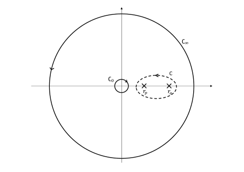
The coefficients , , , and depend only on the energy and angular momentum , and may be considered as mere constants in the present discussion. While , and start at Newtonian order, and are post-Newtonian expressions. By construction, the effective potential (79) vanishes at the periastron and at the apastron , which are the only real roots of the equation . Note that, while logarithmic contributions start at the 3PN order in our Lagrangian-based derivation (since the Lagrangian is defined in harmonic coordinates), they arise only at the 4PN order, and only in the tail part, in our derivation based on the Hamiltonian in ADM coordinates.
To compute (78), we invoke the procedure described in Ref. Damour and Schäfer (1988). The first step consists in choosing one branch cut for , regarded as a function of over the complex plane, to be along the real segment on the real axis. Since the values of the integrand over and under that segment are opposite to each other, the original integral (78) is equal to half the corresponding contour integral over a closed path that surrounds the real segment anti-clockwise (see Fig. 1):
| (80) |
In a second step, we perform the post-Newtonian expansion of under the integration symbol up to the 4PN order, holding the contour fixed. This yields a linear combination of elementary integrals of two types, namely
| (81a) | ||||
| (81b) | ||||
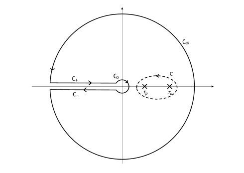
The constants and are explicitly given by and , see Eq. (63), and both are positive: . For the integrals , we finally deform the integration path to the contour displayed in the left panel of Fig. 1, as in the method originally devised by Sommerfeld Sommerfeld (1969).
|
The computation of then amounts to a straightforward application of the residue theorem (see Ref. Damour and Schäfer (1988) for more details).
The integrals have to be handled more carefully. The crucial point is that we must change the way is deformed so as to avoid the branch cut due to the logarithm of on the axis. The final contour in the complex plane is now replaced by the one shown on the right panel of Fig. 1. Let us decompose it into the four different paths , , and as depicted on the figure. They respectively correspond to the contours around zero, below the branch cut, above the branch cut, and at infinity. This decomposition induces the corresponding splitting
| (82) |
On , we can write with a small positive number and going from to ,101010Strictly speaking, we should first integrate with going from to , and then take the limit in the end. We have checked that the end result comes out the same. so that the logarithm becomes . We are led to
| (83) |
After expanding the above expression in powers of , the resulting integrals are immediate to evaluate. For example, when and , we obtain
| (84) |
As for the integrals at infinity that we have to consider, they are all zero:
| (85) |
We are left with the two integrals under and over the branch cut . On the contour , we use the parametrization , for going from to some radius , with and . Similarly, on the contour we take , for going from to . The difference of is due to the presence of the branch cut for the complex logarithm. Adding the two integrals, we get
| (86) |
As one can see, the logarithms have canceled out. In the end, there remains a well-known, tabulated integral Gradshteyn and Ryzhik (1980). For example, for and , we find
| (87) |
Finally, it remains to add all the different pieces and take the limits and .
References
- Bernard et al. (2016a) L. Bernard, L. Blanchet, A. Bohé, G. Faye, and S. Marsat, Phys. Rev. D 93, 084037 (2016a), eprint arXiv:1512.02876 [gr-qc].
- Blanchet (2014) L. Blanchet, Living Rev. Rel. 17, 2 (2014), eprint arXiv:1310.1528 [gr-qc].
- Jaranowski and Schäfer (1998) P. Jaranowski and G. Schäfer, Phys. Rev. D 57, 7274 (1998), eprint gr-qc/9712075.
- Jaranowski and Schäfer (1999) P. Jaranowski and G. Schäfer, Phys. Rev. D 60, 124003 (1999), eprint gr-qc/9906092.
- Jaranowski and Schäfer (2000) P. Jaranowski and G. Schäfer, Ann. Phys. (Berlin) 9, 378 (2000), eprint gr-qc/0003054.
- Damour et al. (2000) T. Damour, P. Jaranowski, and G. Schäfer, Phys. Rev. D 62, 021501(R) (2000), erratum Phys. Rev. D 63, 029903(E) (2000), eprint gr-qc/0003051.
- Damour et al. (2001a) T. Damour, P. Jaranowski, and G. Schäfer, Phys. Rev. D 63, 044021 (2001a), erratum Phys. Rev. D 66, 029901(E) (2002), eprint gr-qc/0010040.
- Damour et al. (2001b) T. Damour, P. Jaranowski, and G. Schäfer, Phys. Lett. B 513, 147 (2001b), eprint gr-qc/0105038.
- Blanchet and Faye (2000a) L. Blanchet and G. Faye, Phys. Lett. A 271, 58 (2000a), eprint gr-qc/0004009.
- Blanchet and Faye (2001) L. Blanchet and G. Faye, Phys. Rev. D 63, 062005 (2001), eprint gr-qc/0007051.
- Blanchet and Faye (2000b) L. Blanchet and G. Faye, J. Math. Phys. 41, 7675 (2000b), eprint gr-qc/0004008.
- de Andrade et al. (2001) V. de Andrade, L. Blanchet, and G. Faye, Class. Quant. Grav. 18, 753 (2001), eprint gr-qc/0011063.
- Blanchet and Iyer (2003) L. Blanchet and B. R. Iyer, Class. Quant. Grav. 20, 755 (2003), eprint gr-qc/0209089.
- Blanchet et al. (2004) L. Blanchet, T. Damour, and G. Esposito-Farèse, Phys. Rev. D 69, 124007 (2004), eprint gr-qc/0311052.
- Itoh et al. (2000) Y. . Itoh, T. Futamase, and H. Asada, Phys. Rev. D 62, 064002 (2000), eprint gr-qc/9910052.
- Itoh et al. (2001) Y. Itoh, T. Futamase, and H. Asada, Phys. Rev. D 63, 064038 (2001), eprint gr-qc/0101114.
- Itoh and Futamase (2003) Y. Itoh and T. Futamase, Phys. Rev. D 68, 121501(R) (2003), eprint gr-qc/0310028.
- Itoh (2004) Y. Itoh, Phys. Rev. D 69, 064018 (2004), eprint gr-qc/0310029.
- Futamase and Itoh (2007) T. Futamase and T. Itoh, Living Rev. Rel. 10, 2 (2007).
- Foffa and Sturani (2011) S. Foffa and R. Sturani, Phys. Rev. D 84, 044031 (2011), eprint arXiv:1104.1122 [gr-qc].
- Jaranowski and Schäfer (2012) P. Jaranowski and G. Schäfer, Phys. Rev. D 86, 061503(R) (2012), eprint arXiv:1207.5448 [gr-qc].
- Jaranowski and Schäfer (2013) P. Jaranowski and G. Schäfer, Phys. Rev. D 87, 081503(R) (2013), eprint arXiv:1303.3225 [gr-qc].
- Jaranowski and Schäfer (2015) P. Jaranowski and G. Schäfer, Phys. Rev. D 92, 124043 (2015), eprint arXiv:1508.01016 [gr-qc].
- Foffa and Sturani (2012) S. Foffa and R. Sturani, Phys. Rev. D 87, 064011 (2012), eprint arXiv:1206.7087 [gr-qc].
- Damour et al. (2014) T. Damour, P. Jaranowski, and G. Schäfer, Phys. Rev. D 89, 064058 (2014), eprint arXiv:1401.4548 [gr-qc].
- Damour et al. (2016) T. Damour, P. Jaranowski, and G. Schäfer, Phys. Rev. D 93, 084014 (2016), eprint arXiv:1601.01283 [gr-qc].
- Blanchet and Damour (1988) L. Blanchet and T. Damour, Phys. Rev. D 37, 1410 (1988).
- Blanchet (1993) L. Blanchet, Phys. Rev. D 47, 4392 (1993).
- Detweiler (2011) S. Detweiler, in Mass and motion in general relativity, edited by L. Blanchet, A. Spallicci, and B. Whiting (Springer, 2011), p. 271.
- Barack (2011) L. Barack, in Mass and motion in general relativity, edited by L. Blanchet, A. Spallicci, and B. Whiting (Springer, 2011), p. 327.
- Blanchet et al. (2010) L. Blanchet, S. Detweiler, A. Le Tiec, and B. Whiting, Phys. Rev. D 81, 084033 (2010), eprint arXiv:1002.0726 [gr-qc].
- Le Tiec et al. (2012a) A. Le Tiec, L. Blanchet, and B. Whiting, Phys. Rev. D 85, 064039 (2012a), eprint arXiv:1111.5378 [gr-qc].
- Le Tiec et al. (2012b) A. Le Tiec, E. Barausse, and A. Buonanno, Phys. Rev. Lett. 108, 131103 (2012b), eprint arXiv:1111.5609 [gr-qc].
- Bini and Damour (2013) D. Bini and T. Damour, Phys. Rev. D 87, 121501(R) (2013), eprint arXiv:1305.4884 [gr-qc].
- Barack et al. (2010) L. Barack, T. Damour, and N. Sago, Phys. Rev. D 82, 084036 (2010), eprint arXiv:1008.0935 [gr-qc].
- Le Tiec et al. (2011) A. Le Tiec, A. Mroué, L. Barack, A. Buonanno, H. Pfeiffer, N. Sago, and A. Taracchini, Phys. Rev. Lett. 107, 141101 (2011), eprint arXiv:1106.3278 [gr-qc].
- van de Meent (2016) M. van de Meent (2016), eprint 1610.03497.
- Damour (2010) T. Damour, Phys. Rev. D 81, 024017 (2010), eprint arXiv:0910.5533 [gr-qc].
- Damour et al. (2015) T. Damour, P. Jaranowski, and G. Schäfer, Phys. Rev. D 91, 084024 (2015), eprint arXiv:1502.07245 [gr-qc].
- Le Tiec (2015) A. Le Tiec, Phys. Rev. D 92, 084021 (2015), eprint arXiv:1506.05648 [gr-qc].
- Blanchet and Le Tiec (2016) L. Blanchet and A. Le Tiec (2016), in preparation.
- Blanchet et al. (2002) L. Blanchet, B. R. Iyer, and B. Joguet, Phys. Rev. D 65, 064005 (2002), erratum Phys. Rev. D, 71:129903(E), 2005, eprint gr-qc/0105098.
- Bernard et al. (2016b) L. Bernard, L. Blanchet, A. Bohé, G. Faye, and S. Marsat (2016b), in progress.
- Hadamard (1932) J. Hadamard, Le problème de Cauchy et les équations aux dérivées partielles linéaires hyperboliques (Hermann, Paris, 1932).
- Schwartz (1978) L. Schwartz, Théorie des distributions (Hermann, Paris, 1978).
- Llosa and Vives (1994) J. Llosa and J. Vives, J. Math. Phys. 35, 2856 (1994).
- Ferialdi and Bassi (2012) L. Ferialdi and A. Bassi, Eur. Phys. Lett. 98, 30009 (2012).
- Foffa and Sturani (2013) S. Foffa and R. Sturani, Phys. Rev. D 87, 044056 (2013), eprint arXiv:1111.5488 [gr-qc].
- Galley et al. (2015) C. Galley, A. Leibovich, R. Porto, and A. Ross (2015), eprint arXiv:1511.07379.
- Arun et al. (2008) K. Arun, L. Blanchet, B. R. Iyer, and M. S. Qusailah, Phys. Rev. D 77, 064034 (2008), eprint arXiv:0711.0250 [gr-qc].
- Detweiler (2008) S. Detweiler, Phys. Rev. D 77, 124026 (2008), eprint arXiv:0804.3529 [gr-qc].
- Barack and Sago (2011) L. Barack and N. Sago, Phys. Rev. D 83, 084023 (2011), eprint arXiv:1101.3331 [gr-qc].
- Damour and Schäfer (1988) T. Damour and G. Schäfer, Nuovo Cim. B101, 127 (1988).
- Sommerfeld (1969) A. Sommerfeld, Atombau und Spektrallinien, vol. 1 (Vieweg, Braunschweig, 1969).
- Martín-García et al. (GPL 2002–2012) J. M. Martín-García, A. García-Parrado, A. Stecchina, B. Wardell, C. Pitrou, D. Brizuela, D. Yllanes, G. Faye, L. Stein, R. Portugal, et al., xAct: Efficient tensor computer algebra for Mathematica (GPL 2002–2012), http://www.xact.es/.
- Marchand et al. (2016) T. Marchand, L. Blanchet, and G. Faye, Class. Quant. Grav. 33, 244003 (2016), eprint arXiv:1607.07601 [gr-qc].
- Gradshteyn and Ryzhik (1980) I. Gradshteyn and I. Ryzhik, Table of Integrals, Series and Products (Academic Press, 1980).